A collider test of nano-Hertz gravitational waves from pulsar timing arrays

Abstract

A cosmic first-order phase transition (FOPT) occurring at MeV-scale provides an attractive explanation for the nano-Hertz gravitational wave (GW) background, which is indicated by the recent pulsar timing array data from the NANOGrav, CPTA, EPTA and PPTA collaborations. We propose this explanation can be further tested at the colliders if the hidden sector couples to the Standard Model sector via the Higgs portal. Through a careful analysis of the thermal history in the hidden sector, we demonstrate that in order to explain the observed GW signal, the portal coupling must be sizable so that it can be probed through Higgs invisible decay at the LHC or future lepton colliders such as CEPC, ILC, and FCC-ee. Our research offers a promising avenue to uncover the physical origin of the nano-Hertz GWs through particle physics experiments.

I Introduction

The observation of gravitational waves (GW) from the merger of binary black hole Abbott et al. (2016) opens the gate of GW astronomy, enabling the exploration of the Universe through messengers apart from electromagnetic waves and neutrinos. Due to the weakness of gravity, GW can carry information from the very early stage of the Universe, opening the window to detect the important processes prior to the Big Bang nucleosynthesis (BBN) and Cosmic Microwave Background (CMB), and probe new physics beyond the Standard Model (SM). Recently, four pulsar timing array (PTA) collaborations, namely NANOGrav Agazie et al. (2023), CPTA Xu et al. (2023), EPTA Antoniadis et al. (2023a) and PPTA Reardon et al. (2023), release their new datasets, showing compelling evidences of a stochastic GW background that peaks at $\mathcal{O}(10^{-8})$ Hz. While this can be interpreted as GWs coming from inspiraling supermassive black hole binaries (SMBHBs), new physics also provides attractive explanations Afzal et al. (2023); Antoniadis et al. (2023b); Smarra et al. (2023). Intriguingly, Bayesian analysis of the data favors new physics models over the conventional SMBHB interpretation Afzal et al. (2023).

One promising new physics explanation of the nano-Hertz GW is a first-order phase transition (FOPT) that happens at the MeV-scale temperature, which has been studied in the literature Han et al. (2023); Megias et al. (2023); Fujikura et al. (2023); Zu et al. (2023); Athron et al. (2023a); Yang et al. (2023a); Addazi et al. (2023) (also see Refs. Kobakhidze et al. (2017); Arunasalam et al. (2018); Addazi et al. (2021); Bian et al. (2021); Nakai et al. (2021); Ratzinger and Schwaller (2021); Borah et al. (2021); Freese and Winkler (2022); Ashoorioon et al. (2022); Bringmann et al. (2023); Madge et al. (2023)). In this paper, we consider the GWs induced by the FOPT in a minimal perspective, where the hidden sector only contains a scalar and a dark gauge boson, and it couples to the SM sector via Higgs-portal interactions. We pay particular attention to the connection between the GWs and particle physics, emphasizing the importance of collider experiments as an efficient probe to identify the physical origin of the nano-Hertz GWs.

The coupling strength between the SM Higgs and a MeV-scale hidden sector has been severely constrained by the LHC data. Such a weak interaction suggests the hidden sector may decouple from the SM thermal bath at GeV-scale before the FOPT occurs. Following this early decoupling, the hidden sector generally reaches a lower temperature at late times because the number of SM relativistic degrees of freedom (d.o.f.) drops significantly at around 100 MeV due to the QCD confinement, which in turn reheats the SM sector. Typically, a smaller portal coupling leads to an earlier thermal decoupling and a smaller temperature ratio between the hidden and the SM sectors. However, a smaller temperature ratio reduces the energy fraction of the FOPT in the Universe and hence suppresses the GWs. Consequently, in vast parameter space, the GW signal has a positive correlation with the Higgs portal strength; especially, we find that the recent reported stochastic GW background requires a sizable portal interaction that can be probed by the Higgs invisible decay at the LHC and future colliders such as CEPC, ILC and FCC-ee.

In this work, we adopt the minimal model with a gauged dark $U(1)_{X}$ to demonstrate the connection between collider experiments and GWs. In Section II, we introduce the model and establish the framework for the FOPT calculation. Then in Section III, we derive the thermal evolution of the hidden sector and point out the relation to the Higgs invisible decay. Based on these discussions, we perform the numerical analysis for a few benchmark points, and present the results in Section IV. Finally, the conclusion is given in Section V.

II FOPT and GWs from a minimal dark $U(1)_{X}$ scenario

We consider a new physics hidden sector that is gauged under a dark $U(1)_{X}$ symmetry. The relevant Lagrangian is

$$\mathcal{L}\supset D_{\mu}S^{\dagger}D^{\mu}S-V(S,H),$$ (1)

where $H=(G^{+},(h+iG^{0})/\sqrt{2})$ is the SM Higgs doublet, $S=(\phi+i\eta)/\sqrt{2}$ is the dark scalar field that is a singlet under the SM gauge group but carries unit charge under the $U(1)_{X}$, and $D_{\mu}=\partial_{\mu}-ig_{X}A^{\prime}_{\mu}$ is the dark covariant derivative with $g_{X}$ being the gauge coupling and $A^{\prime}_{\mu}$ the dark gauge boson. The hidden sector is assumed to interact with the SM sector only through the Higgs portal coupling, which is described by the joint potential

$$V(H,S)=\mu_{h}^{2}|H|^{2}+\mu_{s}^{2}|S|^{2}\\ +\lambda_{h}|H|^{4}+\lambda_{s}|S|^{4}+\lambda_{hs}|H|^{2}|S|^{2}.$$ (2)

The scalars develop vacuum expectation values (VEVs) at $(h,\phi)=(v_{\rm ew},v_{s})$ which break the electroweak (EW) and $U(1)_{X}$ gauge symmetries. The dark gauge boson then acquires a mass $m_{A^{\prime}}=g_{X}v_{s}$.

The coefficients $\{\mu_{h}^{2},\mu_{s}^{2},\lambda_{h},\lambda_{s},\lambda_{hs}\}$ in potential Eq. (2) can be re-parametrized using the physical observables $\{m_{h},v_{\rm ew},m_{\phi},v_{s},\theta\}$, where $\theta$ is the mixing angle between the Higgs boson $h$ and the dark scalar $\phi$. Given $m_{h}=125.09$ GeV and $v_{\rm ew}=246$ GeV, there are three free parameters in $V(H,S)$, and $|\theta|\ll 1$ is required by the Higgs and EW measurements. The details of the re-parametrization of the potential can be found in Appendix A. Here we focus on the MeV-scale hidden FOPT well below the EW symmetry breaking and hence $h\to v_{\rm ew}$. Therefore, the tree-level potential at zero temperature can be matched to

$$V_{0}(\phi)\approx\frac{m_{\phi}^{2}}{8v_{s}^{2}}(\phi^{2}-v_{s}^{2})^{2},$$ (3)

along the $\phi$-direction.

To study the dynamics of the hidden sector in the hot and dense environment of the early Universe, we need to take into account the finite-temperature corrections. Here we denote the temperatures in the hidden and SM sectors as $T^{\prime}$ and $T$, respectively, and allow $\xi\equiv T^{\prime}/T$ to deviate from 1, and $\xi$ itself also varies during the cosmic evolution. The effective $\phi$-potential at finite temperatures is

$$V_{\rm eff}(\phi,T^{\prime})=V_{0}(\phi)+V_{\rm CW}(\phi)+V_{T}(\phi,T^{\prime}),$$ (4)

where $V_{\rm CW}\equiv V_{1}(\phi)+\delta V(\phi)$ is the Coleman-Weinberg potential at zero temperature with the counterterm $\delta V(\phi)$ attached, and $V_{T}(\phi,T^{\prime})\equiv V_{1T}(\phi,T^{\prime})+V_{\rm daisy}(\phi,T^{\prime})$ is the one-loop thermal correction plus the daisy resummation term. See Appendix B for the complete expressions.

FOPT occurs when the Universe transitions from a false vacuum (local minimum) to a true vacuum (global minimum). Initially, the Universe retains at $\phi=0$ due to the behavior of $V_{\rm eff}(\phi,T^{\prime})\approx(-m_{\phi}^{2}+g_{X}^{2}T^{\prime 2}/2)\phi^{2}/4$ at $\phi\sim 0$, which exhibits a valley for high enough $T^{\prime}$. The $U(1)_{X}$ symmetry is preserved at this stage. However, as $T^{\prime}$ decreases, another local minimum at $\phi\neq 0$ emerges and becomes the true vacuum. In certain parameter space, a barrier formed mainly by $A^{\prime}$ in the thermal loop separates the two minima, preventing a smooth transition. In such cases, the Universe undergoes quantum tunneling to the true vacuum, resulting in a $U(1)_{X}$-breaking FOPT with bubble nucleation and expansion dynamics.

We briefly describe the FOPT and GW calculation framework. Bubbles containing the $U(1)_{X}$-breaking vacuum start to nucleate at $T^{\prime}_{n}$ when the decay probability in a Hubble volume and Hubble time reaches $\mathcal{O}(1)$, i.e.

$$\Gamma(T^{\prime}_{n})H^{-4}(T_{n})\approx 1,$$ (5)

where decay rate per unit volume and unit time is

$$\Gamma(T^{\prime})\approx T^{\prime 4}\left(\frac{S_{3}}{2\pi T^{\prime}}\right)^{3/2}e^{-S_{3}/T^{\prime}},$$ (6)

derived by the $T^{\prime}$-dependent action $S_{3}$ of the $O(3)$-symmetric bounce solution Linde (1983). The Hubble constant is dominated by the SM sector, i.e.

$$H(T)\approx 2\pi\sqrt{\frac{\pi g_{*}(T)}{45}}\frac{T^{2}}{M_{\rm Pl}},$$ (7)

where $M_{\rm Pl}=1.22\times 10^{19}$ GeV is the Planck mass and $g_{*}(T)=g_{*,{\rm SM}}(T)+g^{\prime}_{*}(T^{\prime})\xi^{4}$ includes both the relativistic d.o.f. of the SM and hidden sectors. We have assumed a mild FOPT such that the Hubble constant is dominated by the radiation energy throughout the transition, and hence nucleation usually ensures the completion of the FOPT Ellis et al. (2019a). Therefore, Eq. (5) can be adopted as the FOPT criterion, and numerically it implies

$$\frac{S_{3}}{T^{\prime}_{n}}\approx 4\log\left(\frac{1}{4\pi}\sqrt{\frac{45}{\pi g_{*}(T_{n})}}\frac{M_{\rm Pl}}{T^{\prime}_{n}}\xi_{n}^{2}\right),$$ (8)

where $T^{\prime}_{n}$ is the nucleation temperature in the hidden sector, while $T_{n}=T^{\prime}_{n}/\xi_{n}$ is the corresponding SM temperature, and $\xi_{n}\equiv\xi|_{T=T_{n}}$. For an MeV-scale FOPT, $g_{*}(T_{n})\sim 10$ and $S_{3}/T^{\prime}_{n}\approx 190$.

FOPTs source stochastic GWs via bubble collisions, sound waves and turbulence in the plasma Athron et al. (2023b). The key variables describing the GW spectrum are $\{\alpha,\beta/H_{n},T_{n},v_{w}\}$, where

$$\alpha=\frac{1}{g_{*}(T_{n})\pi^{2}T_{n}^{4}/30}\left(T^{\prime}\frac{\partial\Delta V_{\rm eff}}{\partial T^{\prime}}-\Delta V_{\rm eff}\right)\Big{|}_{T^{\prime}_{n}},$$ (9)

with $\Delta V_{\rm eff}<0$ being the energy difference between the true and false vacua. In other words, $\alpha$ is the ratio of the FOPT latent heat to the radiation energy, and it can be factorized as

$$\alpha=\frac{g^{\prime}_{*}(T^{\prime}_{n})}{g_{*}(T_{n})}\alpha^{\prime}\times\xi_{h}^{4},$$ (10)

where $\alpha^{\prime}$ is the latent heat over the hidden radiation energy, and $g^{\prime}_{*}(T^{\prime}_{n})=2+2=4$ is the number of hidden relativistic d.o.f. before the FOPT. By this factorization, we can calculate $\alpha^{\prime}$ with the hidden sector observables alone and then convert it to $\alpha$ for GW calculation. Normally, $\alpha^{\prime}\lesssim 1$ for a non-supercooled FOPT. On the other hand, the $\beta/H_{n}$ parameter, defined as the inverse ratio of the FOPT duration $\beta^{-1}$ to the Hubble time $H_{n}^{-1}\equiv H^{-1}(T_{n})$, can be calculated using only the hidden observables

$$\frac{\beta}{H_{n}}=T^{\prime}_{n}\frac{\text{d}(S_{3}/T^{\prime})}{\text{d}T^{\prime}}\Big{|}_{T^{\prime}_{n}},$$ (11)

due to the cancellation of $\xi_{n}$ factor in the definition Breitbach et al. (2019).

After nucleation, the bubbles undergo an accelerating expansion driven by the vacuum pressure. In the case of a mild FOPT where $\alpha\lesssim 1$, the friction force exerted by $A^{\prime}$ and $\phi$ in the plasma quickly balances the vacuum pressure, resulting in a terminal wall velocity $v_{w}<1$. As a result, most of the vacuum energy released during the FOPT is transferred to plasma motion. Therefore, GWs are primarily generated by sound waves, with turbulence playing a secondary role, while the contribution from bubble collisions is negligible Ellis et al. (2019b). In our research, we adopt $v_{w}=0.9$ as a benchmark.

The GW spectrum from sound wave at production can be expressed as Hindmarsh et al. (2015)

$$\begin{split}\Omega_{{\rm GW},n}=&~{}\frac{1}{\rho_{c,n}}\frac{\text{d}\rho_{{\rm GW},n}}{\text{d}\log f}\\ \approx&~{}1.59\times 10^{-1}\times v_{w}\left(\frac{\kappa_{\rm sw}\alpha}{1+\alpha}\right)^{2}\left(\frac{\beta}{H_{n}}\right)^{-1}\\ &~{}\times\left(\frac{f}{f_{\rm sw}}\right)^{3}\left(\frac{7}{4+3(f/f_{\rm sw})^{2}}\right)^{7/2},\end{split}$$ (12)

where $\kappa_{\rm sw}$ is the fraction of vacuum energy that goes to surrounding plasma, which can be derived by resolving the hydrodynamic motion of the fluid Espinosa et al. (2010), $\rho_{c,n}=3M_{\rm Pl}^{2}H_{n}^{2}/(8\pi)$ is the total energy density at $T_{n}$, and the peak frequency is $f_{\rm sw}=2\beta/{\sqrt{3}v_{w}}$. After the cosmological redshift, the GW spectrum today is Breitbach et al. (2019)

$$\begin{split}\Omega_{\rm GW}(f)=&~{}\frac{1}{\rho_{c}}\frac{\text{d}\rho_{\rm GW}}{\text{d}\log f}\\ =&~{}\left(\frac{a_{n}}{a_{0}}\right)^{4}\left(\frac{H}{H_{0}}\right)^{2}\Omega_{{\rm GW},n}\left(\frac{a_{0}}{a_{n}}f\right),\end{split}$$ (13)

where $a_{0}$ and $a_{n}$ are the scale factor today and at FOPT, respectively, and $H_{0}\approx 67~{}{\rm km}/({\rm s}\cdot{\rm Mpc})$ is the current Hubble constant.

Substituting relevant astrophysical constants into the above equations, we obtain the numerical relation

$$\Omega_{\rm GW}(f)h^{2}\approx 1.238\times 10^{-5}\times\left(g_{*,{\rm SM}}(T_{n})+g^{\prime}_{*}(T^{\prime}_{n})\xi_{n}^{4}\right)\\ \times\left(\frac{g_{*s,{\rm SM}}(T_{0})}{g_{*s,{\rm SM}}(T_{n})+g^{\prime}_{*s}(T^{\prime}_{n})\xi_{n}^{3}}\right)^{4/3}\Omega_{{\rm GW},n}\left(\frac{a_{0}}{a_{n}}f\right),$$ (14)

where $h=H_{0}/[100~{}{\rm km}/({\rm s}\cdot{\rm Mpc})]$, the $g_{*}$’s labeled by a subscript “$s$” denote the d.o.f. related to entropy, for example $g_{*s,{\rm SM}}(T_{0})\approx 3.91$ is the entropy d.o.f. today, and $g_{*,{\rm SM}}(T_{n})=g_{*s,{\rm SM}}(T_{n})=10.75$ for $T_{n}\gtrsim 0.5$ MeV while $g_{*,{\rm SM}}(T_{n})\approx 3.36$ and $g_{*s,{\rm SM}}(T_{n})\approx 3.91$ for $T_{n}\lesssim 0.5$ MeV. By this procedure we can calculate the spectrum $\Omega_{\rm GW}(f)h^{2}$ after solving the thermal history of the hidden sector. The peak frequency after redshift is

$$\left(\frac{a_{n}}{a_{0}}\right)f_{\rm sw}\approx 1.3\times 10^{-8}~{}{\rm Hz}~{}\times\\ \frac{1}{v_{w}}\left(\frac{\beta/H_{n}}{10}\right)\left(\frac{T_{n}}{10~{}{\rm MeV}}\right),$$ (15)

from which we can clearly see the relation between the reported $\sim 10^{-8}$ Hz signal and an MeV-scale $T_{n}$. To include the finite lifetime of the sound wave period, we multiply Eq. (12) with an extra factor $H\tau_{\rm sw}\leqslant 1$ Guo et al. (2021). The sub-leading turbulence contribution is calculated using numerical results Binetruy et al. (2012).

III Thermal history of the hidden sector

The Higgs-portal interactions mediated by $\lambda_{hs}$ in Eq. (2) ensure that the hidden sector remains in equilibrium with the SM sector at high temperatures. In the temperature range ${\rm MeV}\lesssim T\ll 100~{}{\rm GeV}$, specifically after the EW symmetry breaking and before the FOPT, thermal contact is maintained through the Higgs induced process: $SS^{\dagger}\to h^{*}\to$ SM particle pairs. The thermally averaged rate for this process, denoted as $\Gamma_{SS^{\dagger}}$, scales as $\lambda_{hs}^{2}T^{5}/m_{h}^{4}$, so that it decreases more rapidly than the Hubble expansion rate $H(T)\propto T^{2}/M_{\rm Pl}$. When $\Gamma_{SS^{\dagger}}/H$ drops below 1, the hidden sector decouples from the SM plasma and evolves with its own temperature $T^{\prime}$, which might differ from the SM sector temperature $T$.

After the decoupling, the hidden sector typically has a lower temperature $T^{\prime}<T$. This is because the SM sector is reheated when there is a particle species that decouples from the plasma. Such an effect can be calculated via entropy conservation before and after the decoupling, and it is prominent especially at $T\sim 100$ MeV when the quarks and gluons are confined into hadrons, and $g_{*}(T)$ drops drastically from 61.75 to 10.75. In contrast, the hidden sector does not have such reheating effects as it contains only $S$ and $A$. Therefore $\xi_{n}<1$, which suppresses the $\alpha$ parameter by a factor of $\xi_{n}^{4}$, as indicated by Eq. (10); this further suppresses the GW peak signal by

$$\Omega_{\rm GW}\to\xi_{n}^{8}\Omega_{\rm GW},$$ (16)

which can be inferred from Eq. (12). Therefore, a moderate $\xi_{n}\sim 1/2$ can already suppress the GW signal strength by a factor of $10^{-3}$, and hence deriving $\xi_{n}$ is very important in the calculation of the FOPT GW spectrum.

$\xi_{n}$ is determined by evolving the hidden and SM sectors below the decoupling temperature $T_{\rm dec}$, which is resolved by

$$\Gamma_{SS^{\dagger}}(T_{\rm dec})=H(T_{\rm dec}).$$ (17)

below this temperature, the above equality becomes a less-than sign, and the thermal contact is lost. When resolving $T_{\rm dec}$, we consider the annihilation of $SS^{\dagger}\to h^{*}\to$ a pair of SM particles including electrons, muons, pions and kaons, and the relevant meson interaction vertices are taken from Ref. Ibe et al. (2022). Below $T_{\rm dec}$, the two sectors evolve separately and the entropy in either sector conserves, and hence

$$\xi(T)=\left(\frac{g_{*s,{\rm SM}}(T)}{g_{*s,{\rm SM}}(T_{\rm dec})}\right)^{1/3},$$ (18)

which is smaller than 1 when $T<T_{\rm dec}$ and $g_{*s}(T)$ drops below $g_{*s}(T_{\rm dec})$.

The zero-temperature scalar-Higgs mixing angle $\theta$ is crucial in evaluating $T_{\rm dec}$, as the relevant annihilation processes are mediated by an off-shell Higgs boson and hence has a $\Gamma_{SS^{\dagger}}\sim\lambda_{hs}^{2}T^{5}/m_{h}^{4}$ scaling, while $\lambda_{hs}$ is related to the zero-temperature via

$$\lambda_{hs}\approx\frac{m_{\phi}^{2}-m_{h}^{2}}{v_{\rm EW}v_{s}}\theta.$$ (19)

See also the details in Appendix A. In general, a larger $\theta$ results in a larger annihilation rate and consequently a $T_{\rm dec}$ closer to $T_{n}$, which then gives a larger $\xi_{n}$, relaxing the suppression on the GW signals. Therefore, the observed GW background favors a large $\theta$. However, $\theta$ also controls the Higgs exotic decay partial width by

$$\Gamma(h\to 2\phi)=\frac{\theta^{2}m_{h}}{32\pi}\frac{m_{h}^{2}}{v_{s}^{2}}\left(1+\frac{2m_{\phi}^{2}}{m_{h}^{2}}\right)^{2}\sqrt{1-\frac{4m_{\phi}^{2}}{m_{h}^{2}}},$$ (20)

and hence is stringently constrained by current experiments.

$\phi$ is not a stable particle in our model, and it decays via the mixing with the Higgs boson. For MeV-scale $\phi$, the decay to $e^{+}e^{-}$ final state dominates, and the corresponding lifetime of $\phi$, as we will see in the next section, is $\mathcal{O}(1)$ s, resulting in Higgs invisible decay signals at colliders. Currently, the ATLAS collaboration sets $\text{BR}(h\to 2\phi)<0.16$ at $95\%$ C.L. by global fits based on the 13 TeV LHC data with an integrated luminosity of 139 fb^-1 ATL (2021), and this is interpreted as an upper bound of $|\theta|\lesssim 10^{-5}$. Future detection from the HL-LHC can reach $\text{BR}(h\to 2\phi)\approx 0.019$ de Blas et al. (2020), and moreover, the future Higgs factories such as CEPC, ILC or FCC-ee can reach $\text{BR}(h\to 2\phi)\sim 10^{-3}$ Tan et al. (2020); Ishikawa (2019); Potter et al. (2022); Cerri et al. (2017), increasing the sensitivity of $\theta$ by at least an order of magnitude. Those collider experiments can efficiently probe the parameter space favored by the nano-Hertz GW signals indicated by the PTA data, as we will show in the next section.

IV Testing the origin of GWs at colliders

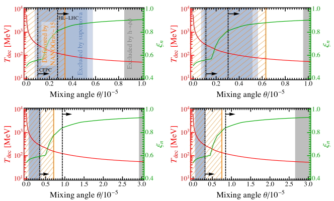
Figure 1: Four BPs: BP1 (top left), BP2 (top right), BP3 (bottom left) and BP4 (bottom right). The $T_{\rm dec}$ and $\xi_{n}$ as functions of $\theta$ are shown as red and green curves, respectively. The region disfavored by the PTA data is covered by orange mesh, while the region excluded by the LHC data is covered by gray. The supernova-excluded region is covered by blue. The projected reach of HL-LHC and CEPC are shown as gray dashed and dotted-dashed vertical lines, respectively.

	$m_{\phi}$ [MeV]	$v_{s}$ [MeV]	$g_{X}$	$\theta_{\rm max}/10^{-5}$	$\alpha$	$\beta/H_{n}$	$T_{n}$ [MeV]
BP1	8.46	42.5	1.01	0.849	0.309	11.2	9.56
BP2	9.16	47.9	0.981	0.955	0.269	8.17	11.2
BP3	23.0	147	0.892	2.93	0.523	12.3	24.3
BP4	31.6	133	1.13	2.66	0.684	16.8	23.9

Table 1: The chosen BPs with the $(m_{\phi},v_{s},g_{X})$ values. $\theta_{\rm max}$ is the maximal $\theta$ allowed by the LHC data, and the subsequent $(\alpha,\beta/H_{n},T_{n})$ is evaluated at $\theta_{\rm max}$.

To quantitatively show our results, for a given parameter set of $(m_{\phi},v_{s},g_{X})$, we use the Python package cosmoTransitions Wainwright (2012) to calculate the bounce action $S_{3}$ and derive $T^{\prime}_{n}$ via Eq. (8). Then a scan on $\theta$ is performed to determine $T_{\rm dec}$ via Eq. (17) and hence $\xi_{n}$ via Eq. (18). We choose four benchmark points (BPs) based on the relatively light ($m_{\phi}\lesssim 10$ MeV) and heavy ($m_{\phi}\gtrsim 20$ MeV) scalar scenarios, as listed in Table 1, and plot $T_{\rm dec}$ and $\xi_{n}$ as functions of $\theta$ in Fig. 1, from which we immediately see the expected negative (positive) correlation of $T_{\rm dec}$ ($\xi_{n}$) to $\theta$. For the parameter space of interest, $T_{\rm dec}$ is at GeV to MeV scale, while $\xi_{n}$ varies from 0.5 to 1. We also notice that $\xi_{n}$ changes rapidly when $T_{\rm dec}$ crosses $\sim 100$ MeV due to the variation of $g_{*}(T)$ caused by QCD confinement, which can be understood from Eq. (18).

Given $\xi_{n}$, we can calculate the GW spectrum as described in Section II, mainly based on the discussions around Eq. (12). The predicted GW signal curve can then be compared with the PTA data from the NANOGrav Agazie et al. (2023) and CPTA Xu et al. (2023) collaborations. For the former, we adopt the $f$-$\Omega_{\rm GW}(f)h^{2}$ data points from Ref. Afzal et al. (2023); while for the latter, we use the the best fit point of $f=14$ nHz and transfer ${\rm log}_{10}A=-14.4^{+1.0}_{-2.8}$ Xu et al. (2023) into $\Omega_{\rm GW}h^{2}$ as an estimate. By varying $\theta$, we see the expected $\xi_{n}^{8}$ suppression effect on the GW signal strength. Hence the parameter space favored by the PTA data exhibits a lower limit for $\theta$, as shown in Fig. 1, where the disfavored regions are covered by orange mesh. By “favored by the PTA data”, we require the GW signals to match the first 14 frequency bins of the NANOGrav-15yr data as they are the most accurate and hence have the largest impact on fit quality, following Ref. Afzal et al. (2023). Currently, both the SMBHB and FOPT interpretations are consistent with the data, although the latter has a higher Bayesian evidence Afzal et al. (2023). Also, the favored FOPT parameter space varies in different fitting setups Afzal et al. (2023); Ellis et al. (2023c); Ghosh et al. (2023); Bian et al. (2023). We expect the future accumulated PTA data could help us to better distinguish the signal origins.

On the other hand, current LHC measurements of Higgs invisible decay set an upper bound $\theta_{\rm max}\sim 10^{-5}$ on the mixing angle, and this is shown as the gray shaded regions in Fig. 1. In addition, a narrow range of $3.9\times 10^{-7}\lesssim\theta\lesssim 7.0\times 10^{-6}$ is excluded by the supernova luminosity limit of SN1987A via the nucleon bremsstrahlung process $NN\to NN\phi$ Dev et al. (2020), as shown in blue shaded regions in the figure. The inner and outer edges correspond to luminosity limit of $5\times 10^{53}~{}{\rm erg/s}$ and $3\times 10^{53}~{}{\rm erg/s}$, respectively.

The FOPT temperatures of our BPs are typically larger than a few MeV, and thus are safe under the BBN and CMB constraints Bai and Korwar (2022); Deng and Bian (2023). The constraints from ultra-compact minihalo (UCMH) abundance Liu et al. (2023); Liu (2023) can also be relaxed by adopting a conservative value of the redshift $z_{c}=1000$ of the last formation of UCHM. The long-lived light scalar $\phi$ with a life time of $\tau_{\phi}\sim\mathcal{O}(1)$ s can affect the BBN process, which in general depends on $m_{\phi}$, $\tau_{\phi}$ and the number density $n_{\phi}$ at decay. Following the analysis of Refs. Hufnagel et al. (2018); Depta et al. (2021), we calculate for each BP the parameter set of $(m_{\phi},\tau_{\phi},n_{\phi})$ and compare with the limits inferred therein. We have checked that all the four BPs are allowed by the BBN constraints.

Combing the above discussions, the regions that are not covered by neither mesh nor colors are viable for explaining the nano-Hertz GW background while being consistent with existing bounds from particle physics, astrophysics and cosmology, opening a window for future experimental exploration. The envelopes of GW spectra of those four BPs within the allowed $\theta$ regions are plotted in Fig. 2, and the corresponding parameters $\alpha$, $\beta/H_{n}$ and $T_{n}$ for the maximally allowed $\theta_{\rm max}$ are listed in Table 1.

We represent the projected reach of $\text{BR}(h\to\phi\phi)$ at the HL-LHC and the CEPC as vertical dashed and dotted-dashed black lines, with 1.9% de Blas et al. (2020) and 0.26% Tan et al. (2020) respectively. The HL-LHC has the capability to explore the entire GW-favored parameter space for BP1 and BP2, as well as a portion of BP3 and BP4. The future CEPC can probe entire allowed parameter space for each of the BPs, and anticipated sensitivities of the ILC and the FCC-ee are comparable Ishikawa (2019); Potter et al. (2022); Cerri et al. (2017). Future multi-TeV muon colliders may even reach an invisible decay branching ratio of $\sim 10^{-4}$, and hence can also test our scenario Ruhdorfer et al. (2023). Therefore, both ongoing and forthcoming collider experiments serve as highly effective means to investigate the physics associated with the nano-Hertz GW background.

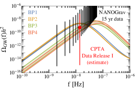
Figure 2: Envelopes of the GW spectra for the BPs in Table 1 when varying $\theta$ within the allowed region. The PTA data are explained in the main text.

V Discussion and conclusion

Before conclusion, we would like to emphasize that the Higgs portal interaction is assumed to be the primary connection between the visible and dark sectors throughout this work. However, there are other possible connections, such as kinetic mixing $\epsilon F^{\prime}_{\mu\nu}F^{\mu\nu}$ between the dark photon $A^{\prime}$ and the SM photon $A$. In this case, a value of $\epsilon\gtrsim 10^{-8}$ can maintain equilibrium between the two sectors via $SS^{\dagger}\to A^{\prime}\to f\bar{f}$ down to MeV-scale temperatures, with $f$ the SM particles. With $10~{}\text{MeV}\lesssim m_{A^{\prime}}\lesssim 100$ MeV favored by PTA data, the current bounds from colliders, beam dump experiments and astrophysics only allow for two ranges of the kinetic mixing: $10^{-5}\lesssim\epsilon\lesssim 10^{-3}$ and $\epsilon\lesssim 10^{-10}$ Fabbrichesi et al. (2020), together with some islands $10^{-14}\lesssim\epsilon\lesssim 10^{-12}$ and $10^{-17}\lesssim\epsilon\lesssim 10^{-16}$ excluded by BBN and CMB observations, respectively Fradette et al. (2014). Therefore, the regime $10^{-5}\lesssim\epsilon\lesssim 10^{-3}$ keeps the two sectors in thermal equilibrium, and consequently the correlation between Higgs invisible decay and the GW signal strength would be lost. In this case, alternate probes could be conducted by focusing on the dark photon Batell et al. (2022). Our scenario of Higgs portal dominance applies when the kinetic mixing falls within the $\epsilon\lesssim 10^{-10}$ range, or it is forbidden by a $\mathbb{Z}_{2}$ symmetry with $A^{\prime}\to-A^{\prime}$ and $S\to S^{\dagger}$ Kanemura et al. (2010); Lebedev et al. (2012).

In either case mentioned above, the dark gauge boson $A^{\prime}$ could be long-lived and contribute to the dark matter relic density at present day. Since $m_{A^{\prime}}>m_{\phi}$, the $A^{\prime}$ will freeze-out via secluded annihilation $A^{\prime}A^{\prime}\to\phi\phi$, with the relic density today scaling like the standard WIMP paradigm:

$$\Omega_{A^{\prime}}h^{2}\approx 0.1\left(\frac{0.1}{g_{X}}\right)^{4}\left(\frac{m_{A^{\prime}}}{100~{}{\rm GeV}}\right)^{2},$$ (21)

which is $\sim 10^{-12}$ for the parameter space of interest, much smaller than the dark matter relic abundance and hence negligible.

In conclusion, we propose a collider test to the nano-Hertz GW signals reported by the recent PTA experiments. Our idea is based on the extensively studied Higgs-portal model, which consists of a hidden sector that is gauged under a dark $U(1)_{X}$. We demonstrate that the explanation of the PTA data requires a sizable Higgs portal coupling, which results in a $h\to\phi\phi$ exotic decay that leads to an invisible final state, and can be probed at the colliders. By choosing several BPs as examples, we show that the HL-LHC is able to efficiently probe the parameter space required by the PTA data, while the future lepton colliders such as CEPC can cover almost all the parameter space of interest. Our research shows the importance of collider experiments in testing the origin of the stochastic GW background.

Appendix A The re-parametrization of the joint potential

In the unitary gauge, $H\to h/\sqrt{2}$ and $S\to\phi/\sqrt{2}$, the potential is rewritten as

$$V(h,\phi)=\frac{\mu_{h}^{2}}{2}h^{2}+\frac{\lambda_{h}}{4}h^{4}+\frac{\mu_{s}^{2}}{2}\phi^{2}+\frac{\lambda_{s}}{4}\phi^{4}+\frac{\lambda_{hs}}{4}h^{2}\phi^{2},$$ (22)

which is minimized at the vacuum $(h,\phi)=(v_{\rm ew},v_{s})$. Given the mass eigenvalues $m_{h}$, $m_{\phi}$ and the mixing angle $\theta$, the coefficients in Eq. (22) can be expressed as

$$\mu_{h,s}^{2}=-\frac{1}{4}\Big{[}m_{h}^{2}+m_{\phi}^{2}\mp(m_{\phi}^{2}-m_{h}^{2})\\ \left(\cos 2\theta\mp\left(\frac{v_{s}}{v_{\rm ew}}\right)^{\pm 1}\sin 2\theta\right)\Big{]},$$ (23)

and

$$\begin{split}\lambda_{h}=&~{}\frac{m_{h}^{2}+m_{\phi}^{2}-(m_{\phi}^{2}-m_{h}^{2})\cos 2\theta}{4v_{\rm ew}^{2}},\\ \lambda_{s}=&~{}\frac{m_{h}^{2}+m_{\phi}^{2}+(m_{\phi}^{2}-m_{h}^{2})\cos 2\theta}{4v_{s}^{2}},\\ \lambda_{hs}=&~{}\frac{(m_{\phi}^{2}-m_{h}^{2})\sin 2\theta}{2v_{\rm ew}v_{s}}.\end{split}$$ (24)

For small mixing angle $|\theta|\ll 1$, the interaction vertices can be read from the following interaction Lagrangian

$$\mathcal{L}_{3}\approx-\frac{m_{h}^{2}}{2v_{\rm ew}}h^{3}+\frac{2m_{h}^{2}+m_{\phi}^{2}}{2v_{\rm ew}}\theta h^{2}\phi\\ +\frac{m_{h}^{2}+2m_{\phi}^{2}}{2v_{s}}\theta h\phi^{2}-\frac{m_{\phi}^{2}}{2v_{s}}\phi^{3},$$ (25)

$$\mathcal{L}_{4}\approx-\frac{m_{h}^{2}}{8v_{\rm ew}^{2}}h^{4}-\frac{m_{h}^{2}}{2v_{\rm ew}^{2}}\theta h^{3}\phi\\ -\frac{m_{\phi}^{2}-m_{h}^{2}}{4v_{\rm ew}v_{s}}\theta h^{2}\phi^{2}+\frac{m_{\phi}^{2}}{2v_{s}^{2}}\theta h\phi^{3}-\frac{m_{\phi}^{2}}{8v_{s}^{2}}\phi^{4},$$ (26)

in which $h$ and $\phi$ should be understood as physical particles.

Appendix B The complete expression of the $V_{\rm eff}(\phi,T^{\prime})$

The finite temperature potential of $\phi$ consists of zero-temperature tree level potential $V_{0}(\phi)$ as given in Eq. (3) of the main text, the one-loop Coleman-Weinberg correction

$$V_{1}(\phi)=\sum_{i=\phi,A^{\prime}}\frac{n_{i}M_{i}^{4}(\phi)}{64\pi^{2}}\left(\log\frac{M_{i}^{2}(\phi)}{\mu_{R}^{2}}-C_{i}\right),$$ (27)

where $\mu_{R}=10$ MeV is the renormalization scale,

$$M_{\phi}^{2}(\phi)=-\frac{m_{\phi}^{2}}{2}+\frac{3m_{\phi}^{2}}{2v_{s}^{2}}\phi^{2},\quad M_{A^{\prime}}(\phi)=g_{X}\phi,$$ (28)

are the field-dependent masses, $n_{\phi,A^{\prime}}=1$, 3 and $C_{\phi,A^{\prime}}=3/2$, $5/6$, respectively. Note that the contribution from the Goldstone $\eta$ is neglected to avoid the IR divergence Espinosa et al. (2012). The counter term $\delta V(\phi)\equiv\delta\mu_{s}^{2}\phi^{2}/2+\delta\lambda_{s}\phi^{4}/4$ is determined by the condition that one-loop zero temperature potential $V_{0}(\phi)+V_{1}(\phi)+\delta V(\phi)$ should still have a VEV at $\left\langle\phi\right\rangle=v_{s}$ with a mass eigenvalue $m_{\phi}$.

The thermal correction at one-loop level is given by

$$V_{T1}(\phi,T^{\prime})=\sum_{i=\phi,\eta,A^{\prime}}\frac{n_{i}T^{\prime 4}}{2\pi^{2}}J_{B}\left(\frac{M_{i}^{2}(\phi)}{T^{\prime 2}}\right),$$ (29)

where $n_{\eta}=1$ and $M_{\eta}^{2}(\phi)=-m_{\phi}^{2}(1-\phi^{2}/v_{s}^{2})/2$, and the Bose thermal integral

$$J_{B}(y)=\int_{0}^{\infty}x^{2}{\rm d}x\log(1-e^{-\sqrt{x^{2}+y}}).$$

The thermal correction is dominated by the $A^{\prime}$ contribution, as $g_{X}^{2}\gg\lambda_{s}$ in the parameter space of interest. The last term, i.e. the daisy resummation, is

$$V_{\rm daisy}(\phi,T^{\prime})=-\frac{g_{X}^{3}T^{\prime}}{12\pi}\left((\phi^{2}+T^{\prime 2})^{3/2}-\phi^{3}\right),$$ (30)

where the sub-leading contributions from $\phi$ and $\eta$ are dropped.

References

- Abbott et al. (2016) B. P. Abbott et al. (LIGO Scientific, Virgo), Phys. Rev. Lett. 116, 061102 (2016), eprint 1602.03837.
- Agazie et al. (2023) G. Agazie et al. (NANOGrav), Astrophys. J. Lett. 951 (2023), eprint 2306.16213.
- Xu et al. (2023) H. Xu et al., Res. Astron. Astrophys. 23, 075024 (2023), eprint 2306.16216.
- Antoniadis et al. (2023a) J. Antoniadis et al. (2023a), eprint 2306.16214.
- Reardon et al. (2023) D. J. Reardon et al. (2023), eprint 2306.16215.
- Afzal et al. (2023) A. Afzal et al. (NANOGrav), Astrophys. J. Lett. 951, L11 (2023), eprint 2306.16219.
- Antoniadis et al. (2023b) J. Antoniadis et al. (2023b), eprint 2306.16227.
- Smarra et al. (2023) C. Smarra et al. (European Pulsar Timing Array) (2023), eprint 2306.16228.
- Han et al. (2023) C. Han, K.-P. Xie, J. M. Yang, and M. Zhang (2023), eprint 2306.16966.
- Megias et al. (2023) E. Megias, G. Nardini, and M. Quiros (2023), eprint 2306.17071.
- Fujikura et al. (2023) K. Fujikura, S. Girmohanta, Y. Nakai, and M. Suzuki (2023), eprint 2306.17086.
- Zu et al. (2023) L. Zu, C. Zhang, Y.-Y. Li, Y.-C. Gu, Y.-L. S. Tsai, and Y.-Z. Fan (2023), eprint 2306.16769.
- Athron et al. (2023a) P. Athron, A. Fowlie, C.-T. Lu, L. Morris, L. Wu, Z. Xu, and Y. Wu (2023a), eprint 2306.17239.
- Yang et al. (2023a) A. Yang, J. Ma, S. Jiang, and F. P. Huang (2023a), eprint 2306.17827.
- Addazi et al. (2023) A. Addazi, Y.-F. Cai, A. Marciano, and L. Visinelli (2023), eprint 2306.17205.
- Kobakhidze et al. (2017) A. Kobakhidze, C. Lagger, A. Manning, and J. Yue, Eur. Phys. J. C 77, 570 (2017), eprint 1703.06552.
- Arunasalam et al. (2018) S. Arunasalam, A. Kobakhidze, C. Lagger, S. Liang, and A. Zhou, Phys. Lett. B 776, 48 (2018), eprint 1709.10322.
- Addazi et al. (2021) A. Addazi, Y.-F. Cai, Q. Gan, A. Marciano, and K. Zeng, Sci. China Phys. Mech. Astron. 64, 290411 (2021), eprint 2009.10327.
- Bian et al. (2021) L. Bian, R.-G. Cai, J. Liu, X.-Y. Yang, and R. Zhou, Phys. Rev. D 103, L081301 (2021), eprint 2009.13893.
- Nakai et al. (2021) Y. Nakai, M. Suzuki, F. Takahashi, and M. Yamada, Phys. Lett. B 816, 136238 (2021), eprint 2009.09754.
- Ratzinger and Schwaller (2021) W. Ratzinger and P. Schwaller, SciPost Phys. 10, 047 (2021), eprint 2009.11875.
- Borah et al. (2021) D. Borah, A. Dasgupta, and S. K. Kang, JCAP 12, 039 (2021), eprint 2109.11558.
- Freese and Winkler (2022) K. Freese and M. W. Winkler, Phys. Rev. D 106, 103523 (2022), eprint 2208.03330.
- Ashoorioon et al. (2022) A. Ashoorioon, K. Rezazadeh, and A. Rostami, Phys. Lett. B 835, 137542 (2022), eprint 2202.01131.
- Bringmann et al. (2023) T. Bringmann, P. F. Depta, T. Konstandin, K. Schmidt-Hoberg, and C. Tasillo (2023), eprint 2306.09411.
- Madge et al. (2023) E. Madge, E. Morgante, C. P. Ibáñez, N. Ramberg, W. Ratzinger, S. Schenk, and P. Schwaller (2023), eprint 2306.14856.
- Guo et al. (2023) S.-Y. Guo, M. Khlopov, X. Liu, L. Wu, Y. Wu, and B. Zhu (2023), eprint 2306.17022.
- Kitajima et al. (2023) N. Kitajima, J. Lee, K. Murai, F. Takahashi, and W. Yin (2023), eprint 2306.17146.
- Bai et al. (2023) Y. Bai, T.-K. Chen, and M. Korwar (2023), eprint 2306.17160.
- Blasi et al. (2023) S. Blasi, A. Mariotti, A. Rase, and A. Sevrin (2023), eprint 2306.17830.
- Sakharov et al. (2021) A. S. Sakharov, Y. N. Eroshenko, and S. G. Rubin, Phys. Rev. D 104, 043005 (2021), eprint 2104.08750.
- Ellis et al. (2023a) J. Ellis, M. Lewicki, C. Lin, and V. Vaskonen (2023a), eprint 2306.17147.
- Wang et al. (2023a) Z. Wang, L. Lei, H. Jiao, L. Feng, and Y.-Z. Fan (2023a), eprint 2306.17150.
- Kitajima and Nakayama (2023) N. Kitajima and K. Nakayama (2023), eprint 2306.17390.
- Lazarides et al. (2023) G. Lazarides, R. Maji, and Q. Shafi (2023), eprint 2306.17788.
- Vagnozzi (2023) S. Vagnozzi (2023), eprint 2306.16912.
- Franciolini et al. (2023a) G. Franciolini, A. Iovino, Junior., V. Vaskonen, and H. Veermae (2023a), eprint 2306.17149.
- Cai et al. (2023) Y.-F. Cai, X.-C. He, X. Ma, S.-F. Yan, and G.-W. Yuan (2023), eprint 2306.17822.
- Oikonomou (2023) V. K. Oikonomou (2023), eprint 2306.17351.
- Wang et al. (2023b) S. Wang, Z.-C. Zhao, J.-P. Li, and Q.-H. Zhu (2023b), eprint 2307.00572.
- Yang et al. (2023b) J. Yang, N. Xie, and F. P. Huang (2023b), eprint 2306.17113.
- Ellis et al. (2023b) J. Ellis, M. Fairbairn, G. Hütsi, J. Raidal, J. Urrutia, V. Vaskonen, and H. Veermäe (2023b), eprint 2306.17021.
- Shen et al. (2023) Z.-Q. Shen, G.-W. Yuan, Y.-Y. Wang, and Y.-Z. Wang (2023), eprint 2306.17143.
- Ghoshal and Strumia (2023) A. Ghoshal and A. Strumia (2023), eprint 2306.17158.
- Broadhurst et al. (2023) T. Broadhurst, C. Chen, T. Liu, and K.-F. Zheng (2023), eprint 2306.17821.
- Inomata et al. (2023) K. Inomata, K. Kohri, and T. Terada (2023), eprint 2306.17834.
- Depta et al. (2023) P. F. Depta, K. Schmidt-Hoberg, and C. Tasillo (2023), eprint 2306.17836.
- Gouttenoire and Vitagliano (2023) Y. Gouttenoire and E. Vitagliano (2023), eprint 2306.17841.
- Huang et al. (2023) H.-L. Huang, Y. Cai, J.-Q. Jiang, J. Zhang, and Y.-S. Piao (2023), eprint 2306.17577.
- Gouttenoire et al. (2023) Y. Gouttenoire, S. Trifinopoulos, G. Valogiannis, and M. Vanvlasselaer (2023), eprint 2307.01457.
- Lambiase et al. (2023) G. Lambiase, L. Mastrototaro, and L. Visinelli (2023), eprint 2306.16977.
- Li et al. (2023) Y. Li, C. Zhang, Z. Wang, M. Cui, Y.-L. S. Tsai, Q. Yuan, and Y.-Z. Fan (2023), eprint 2306.17124.
- Franciolini et al. (2023b) G. Franciolini, D. Racco, and F. Rompineve (2023b), eprint 2306.17136.
- Croon et al. (2021) D. Croon, O. Gould, P. Schicho, T. V. I. Tenkanen, and G. White, JHEP 04, 055 (2021), eprint 2009.10080.
- Linde (1983) A. D. Linde, Nucl. Phys. B 216, 421 (1983), [Erratum: Nucl.Phys.B 223, 544 (1983)].
- Ellis et al. (2019a) J. Ellis, M. Lewicki, and J. M. No, JCAP 04, 003 (2019a), eprint 1809.08242.
- Athron et al. (2023b) P. Athron, C. Balázs, A. Fowlie, L. Morris, and L. Wu (2023b), eprint 2305.02357.
- Breitbach et al. (2019) M. Breitbach, J. Kopp, E. Madge, T. Opferkuch, and P. Schwaller, JCAP 07, 007 (2019), eprint 1811.11175.
- Ellis et al. (2019b) J. Ellis, M. Lewicki, J. M. No, and V. Vaskonen, JCAP 06, 024 (2019b), eprint 1903.09642.
- Hindmarsh et al. (2015) M. Hindmarsh, S. J. Huber, K. Rummukainen, and D. J. Weir, Phys. Rev. D 92, 123009 (2015), eprint 1504.03291.
- Espinosa et al. (2010) J. R. Espinosa, T. Konstandin, J. M. No, and G. Servant, JCAP 06, 028 (2010), eprint 1004.4187.
- Guo et al. (2021) H.-K. Guo, K. Sinha, D. Vagie, and G. White, JCAP 01, 001 (2021), eprint 2007.08537.
- Binetruy et al. (2012) P. Binetruy, A. Bohe, C. Caprini, and J.-F. Dufaux, JCAP 06, 027 (2012), eprint 1201.0983.
- Ibe et al. (2022) M. Ibe, S. Kobayashi, Y. Nakayama, and S. Shirai, JHEP 03, 198 (2022), eprint 2112.11096.
- ATL (2021) Tech. Rep., CERN, Geneva (2021), all figures including auxiliary figures are available at https://atlas.web.cern.ch/Atlas/GROUPS/PHYSICS/CONFNOTES/ATLAS-CONF-2021-053, URL http://cds.cern.ch/record/2789544.
- de Blas et al. (2020) J. de Blas et al., JHEP 01, 139 (2020), eprint 1905.03764.
- Tan et al. (2020) Y. Tan et al., Chin. Phys. C 44, 123001 (2020), eprint 2001.05912.
- Ishikawa (2019) A. Ishikawa, PoS LeptonPhoton2019, 147 (2019), eprint 1909.07537.
- Potter et al. (2022) C. Potter, A. Steinhebel, J. Brau, A. Pryor, and A. White (2022), eprint 2203.08330.
- Cerri et al. (2017) O. Cerri, M. de Gruttola, M. Pierini, A. Podo, and G. Rolandi, Eur. Phys. J. C 77, 116 (2017), eprint 1605.00100.
- Wainwright (2012) C. L. Wainwright, Comput. Phys. Commun. 183, 2006 (2012), eprint 1109.4189.
- Ellis et al. (2023c) J. Ellis, M. Fairbairn, G. Franciolini, G. Hütsi, A. Iovino, M. Lewicki, M. Raidal, J. Urrutia, V. Vaskonen, and H. Veermäe (2023c), eprint 2308.08546.
- Ghosh et al. (2023) T. Ghosh, A. Ghoshal, H.-K. Guo, F. Hajkarim, S. F. King, K. Sinha, X. Wang, and G. White (2023), eprint 2307.02259.
- Bian et al. (2023) L. Bian, S. Ge, J. Shu, B. Wang, X.-Y. Yang, and J. Zong (2023), eprint 2307.02376.
- Dev et al. (2020) P. S. B. Dev, R. N. Mohapatra, and Y. Zhang, JCAP 08, 003 (2020), [Erratum: JCAP 11, E01 (2020)], eprint 2005.00490.
- Bai and Korwar (2022) Y. Bai and M. Korwar, Phys. Rev. D 105, 095015 (2022), eprint 2109.14765.
- Deng and Bian (2023) S. Deng and L. Bian (2023), eprint 2304.06576.
- Liu et al. (2023) J. Liu, L. Bian, R.-G. Cai, Z.-K. Guo, and S.-J. Wang, Phys. Rev. Lett. 130, 051001 (2023), eprint 2208.14086.
- Liu (2023) J. Liu (2023), eprint 2305.15100.
- Hufnagel et al. (2018) M. Hufnagel, K. Schmidt-Hoberg, and S. Wild, JCAP 11, 032 (2018), eprint 1808.09324.
- Depta et al. (2021) P. F. Depta, M. Hufnagel, and K. Schmidt-Hoberg, JCAP 04, 011 (2021), eprint 2011.06519.
- Ruhdorfer et al. (2023) M. Ruhdorfer, E. Salvioni, and A. Wulzer, Phys. Rev. D 107, 095038 (2023), eprint 2303.14202.
- Fabbrichesi et al. (2020) M. Fabbrichesi, E. Gabrielli, and G. Lanfranchi (2020), eprint 2005.01515.
- Fradette et al. (2014) A. Fradette, M. Pospelov, J. Pradler, and A. Ritz, Phys. Rev. D 90, 035022 (2014), eprint 1407.0993.
- Batell et al. (2022) B. Batell, N. Blinov, C. Hearty, and R. McGehee, in Snowmass 2021 (2022), eprint 2207.06905.
- Kanemura et al. (2010) S. Kanemura, S. Matsumoto, T. Nabeshima, and N. Okada, Phys. Rev. D 82, 055026 (2010), eprint 1005.5651.
- Lebedev et al. (2012) O. Lebedev, H. M. Lee, and Y. Mambrini, Phys. Lett. B 707, 570 (2012), eprint 1111.4482.
- Espinosa et al. (2012) J. R. Espinosa, T. Konstandin, and F. Riva, Nucl. Phys. B 854, 592 (2012), eprint 1107.5441.