Using Solar Orbiter as an upstream solar wind monitor for real time space weather predictions
Abstract
Coronal mass ejections (CMEs) can create significant disruption to human activities and systems on Earth, much of which can be mitigated with prior warning of the upstream solar wind conditions. However, it is currently extremely challenging to accurately predict the arrival time and internal structure of a CME from coronagraph images alone. In this study, we take advantage of a rare opportunity to use Solar Orbiter, at 0.5 AU upstream of Earth, as an upstream solar wind monitor. We were able to use real time science quality magnetic field measurements, taken only 12 minutes earlier, to predict the arrival time of a CME prior to reaching Earth. We used measurements at Solar Orbiter to constrain an ensemble of simulation runs from the ELEvoHI model, reducing the uncertainty in arrival time from 10.4 hours to 2.5 hours. There was also an excellent agreement in the profile between Solar Orbiter and Wind spacecraft, despite being separated by 0.5 AU and 10∘ longitude. Therefore, we show that it is possible to predict not only the arrival time of a CME, but the sub-structure of the magnetic field within it, over a day in advance. The opportunity to use Solar Orbiter as an upstream solar wind monitor will repeat once a year, which should further help assess the efficacy upstream in-situ measurements in real time space weather forecasting.
Space Weather
Imperial College London, Blackett Laboratory, South Kensington, SW7 2AZ Austrian Space Weather Office, GeoSphere Austria, Reininghausstraße 3, 8020 Graz, Austria RAL Space, STFC Rutherford Appleton Laboratory, Harwell Campus, Didcot OX11 0QX, UK Hvar Observatory, Faculty of Geodesy, University of Zagreb, Croatia
Ronan Lakerronan.laker15@imperial.ac.uk
Real time data from Solar Orbiter was used to predict the arrival time of a coronal mass ejection at Earth more than a day in advance
In situ measurements at 0.5 AU were used to reduce the mean absolute error in arrival time from 10.4 to 2.5 hours with the ELEvoHI model
The in situ Bz profile was comparable to the geomagnetic response at Earth, despite being separated by 0.5 AU and 10∘ longitude
Plain Language Summary
Coronal mass ejections (CMEs) are large eruptions of plasma from the Sun that can significantly disrupt human technology when directed at Earth. Much like weather on Earth, the consequences of these ‘space weather’ events can be lessened with warning of their arrival, e.g., putting satellites into safe mode. This is usually done by identifying a CME in telescope images, and then predicting if and when it will arrive at Earth. However, the current forecasting models have large uncertainties in arrival time, and struggle to predict the in situ properties of the CME, which can significantly alter the severity of the event. In this paper, by taking advantage of a period in March 2022, we were able to use real time measurements from halfway between the Sun and the Earth taken by the Solar Orbiter spacecraft. This allowed us, for the first time, to predict the arrival time and magnetic structure of a CME, more than a day before it arrived at Earth. We also show that the Solar Orbiter measurements can be used to constrain a CME propagation model, significantly improving the accuracy and precision of the forecasted arrival time.
1 Introduction
Space weather can create significant disruption to human technology both in space and on Earth, including loss of satellites, damage to power grids and communication blackouts [Hapgood (\APACyear2012), Eastwood, Biffis\BCBL \BOthers. (\APACyear2017)]. Fortunately, many of these effects can be mitigated with prior warning, meaning that timely and accurate predictions of the arrival and severity of space weather events are extremely important [Eastwood, Nakamura\BCBL \BOthers. (\APACyear2017)].
The majority of severe geomagnetic storms at Earth are driven by coronal mass ejections [<]CMEs,¿[]Richardson2001, large and complex structures impulsively released from the Sun’s corona. Remote sensing observations of the corona can reveal the release of a CME from the Sun, whose propagation through the ambient solar wind can then be simulated to predict an arrival time at Earth. While there are many sophisticated solar wind and CME models, they often have arrival time errors of hours, partly due to uncertain estimates of the CME’s initial parameters [Riley \BOthers. (\APACyear2018), Wold \BOthers. (\APACyear2018)]. In addition, the interaction between the CME and the ambient solar wind can deflect, deform and rotate the CME, which can also significantly affect the arrival time [Wang \BOthers. (\APACyear2002), Wang \BOthers. (\APACyear2004), Gui \BOthers. (\APACyear2011), Good \BOthers. (\APACyear2019), Desai \BOthers. (\APACyear2020)].
Information regarding the orientation of the CME’s magnetic field, a primary indicator of geo-effectiveness, is often as valuable as the predictions of arrival time [Owens, Lockwood\BCBL \BBA Barnard (\APACyear2020)]. Knowing the potential impact of the CME, rather than just its arrival time, can limit the number of false positives and make predictions more useful for those commercial applications where there is a high cost of mitigation, e.g., putting a spacecraft into a safe mode. Currently, information about the internal magnetic structure and plasma parameters of an earth-directed CME are provided by a number of spacecraft at L1: Wind, ACE and DSCOVR. However, their placement just ahead of Earth only provides a lead time of around an hour, which is often not long enough to take appropriate mitigating measures.
To address many of the problems with the current prediction framework, future upstream solar wind monitors have been proposed, which would be positioned further from Earth than L1. However, such a mission would rely on currently inaccessible solar sail technology or a large constellation of orbiting probes [Heiligers \BBA McInnes (\APACyear2014)], meaning that there are still open questions regarding the efficacy of these future proposals. In the case of the probe constellation, it would be useful to know the minimum separation in longitude that would provide continuous prediction capabilities. In addition, the optimal position for a spacecraft would be a trade-off between improved lead time and the accuracy of the prediction. For example, placing a spacecraft within Mercury’s orbit would give several days lead time, but the solar wind structures seen by the spacecraft may have evolved significantly after travelling to Earth. While several case studies have already shown how an upstream spacecraft can be useful in predicting the arrival time and geo-effectiveness [Lindsay \BOthers. (\APACyear1999), Rollett \BOthers. (\APACyear2014), Kubicka \BOthers. (\APACyear2016), Amerstorfer \BOthers. (\APACyear2018)], such a concept has never been attempted in real time.
In this paper, we take advantage of an unprecedented opportunity to use Solar Orbiter [Müller \BOthers. (\APACyear2020)] as a real time upstream solar wind monitor. During a period between February and March 2022, Solar Orbiter crossed the Sun-Earth line at a heliocentric distance of AU, observing two CMEs in situ and, for the first time, providing predictions of the arrival time and magnetic structure before they arrived at Earth. In Section 2, we outline the operational constraints of the Solar Orbiter mission for this purpose and also detail the models used for arrival time prediction. We then present the results of our two CME case studies in Section 3.1, showing how these measurements can be used to improve the uncertainty in predicted arrival time prior to reaching Earth. Finally, the similarity of the magnetic field structure at 0.5 AU and Earth is investigated in Section 3.2, opening up the possibility to predict the sub-structure of a CME event, not just the arrival time.
2 Methodology
2.1 Operations
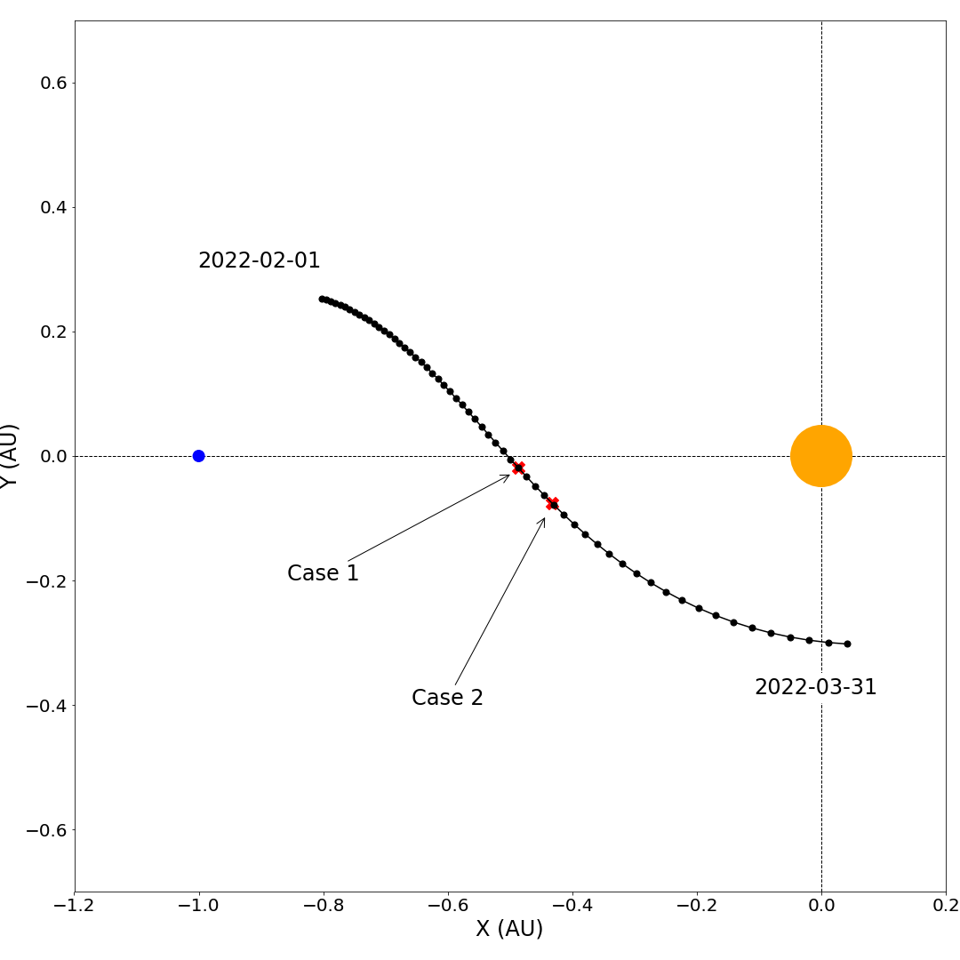
During February and March 2022 Solar Orbiter travelled from AU to AU heliocentric distance, crossing the Sun-Earth line on 6 March 2022, as summarised by Fig. 1. While the spacecraft has crossed the Sun-Earth line before, for this crossing, Solar Orbiter had the capability to return data sufficiently quickly to predict the onset and severity of geomagnetic storms at Earth. This was made possible by the low latency data products returned by the instruments at 100 bits/second, which are intended to help with the ‘very short term planning’ of the remote sensing instruments – pointing them in the direction of relevant solar structures, such as active regions or the polar coronal holes [Müller \BOthers. (\APACyear2020), Auchère \BOthers. (\APACyear2020)].
Since Solar Orbiter was not designed to be an upstream solar wind monitor, there were a few operational constraints that affected our prediction capability. First, the data was only downloaded in an -hour window per day, referred to as a ‘pass’. Therefore, if a CME arrived between passes, we could not provide predictions until the next pass began, which could be up to hours later. Under normal operation, the low latency data taken between passes is downloaded within 30 minutes of the start of the next pass, while within the pass the latency is less than 5 minutes. Since this is only intended to be quick look data for short term planning, this data typically still has artefacts that make it unsuitable for science.
To overcome these challenges, the Solar Orbiter MAG team [Horbury \BOthers. (\APACyear2020)] created a pipeline to produce real time data that was closer to science quality. Housekeeping data, provided in the low latency packets, was used to remove over different heater signals from the spacecraft, as well as interference from other instruments aboard Solar Orbiter [Angelini \BOthers. (\APACyear2022)]. This custom pipeline was then run on demand during the pass, and could achieve a latency of just minutes from taking the measurement to being science quality on the ground, which included a -minute light travel time. However, for the purposes of this study, the real time data was only available for the magnetic field, with the plasma data from the Proton Alpha Sensor [<]PAS, ¿[]Owen2020 becoming available at the end of the -hour pass. With Solar Orbiters position, our lead time would be around hours for a km/s CME at AU, meaning that in practice we still had access to the plasma data before the CME arrived at Earth. For future radial alignments, both plasma and magnetic field data will be available in real time.
| Timings | Case 1 | Case 2 |
| CME launch time (STEREO-A) | 2022-03-05 18:00 | 2022-03-10 19:30 |
| Solar Orbiter in situ observation | 2022-03-07 22:49 | 2022-03-11 19:52 |
| Distance to Sun | AU | AU |
| Angle to Sun-Earth line | ||
| Earth estimated arrival time (PAS speed) | 2022-03-10 19:54hrs | 2022-03-13 10:18hrs |
| Earth modelled arrival time (ELEvoHI) | 2022-03-11 01:04 | 2022-03-13 13:01 |
| ME, MAE | hrs, hrs | hrs, hrs |
| Earth modelled arrival time (constrained ELEvoHI) | 2022-03-10 14:07 | 2022-03-13 10:25 |
| ME, MAE | hrs, hrs | hrs, hrs |
| Earth arrival time (corrected from Wind to Earth) | 2022-03-10 16:59 | 2022-03-13 10:53 |
2.2 Modelling
After identifying a CME within the Solar Orbiter in situ data, we then attempted to predict its arrival time at Earth. As well as providing an estimate simply using distance divided by speed from PAS, which inherently neglects effects such as drag, we also applied the ELEvoHI model in real time [Rollett \BOthers. (\APACyear2016), Amerstorfer \BOthers. (\APACyear2018)]. With this particular model, it was not just a fortunate line-up between Solar Orbiter and Earth, but the position of STEREO-A was such that it could provide a side view of any CMEs directed towards Solar Orbiter. A full description of this model, and the underlying assumptions, can be found in \citeAAmerstorfer2021 and \citeABauer2021.
In essence, this model first uses the heliospheric imager [<]HI,¿[]Eyles2009 data from STEREO-A to obtain an elongation track that is then converted to radial distance using the ELlipse Conversion method [<]ELCon,¿[]Rollett2016. Tracing the CME front, and fitting the time-distance profile with a drag based model [<]DBM,¿[]Vrsnak2013, allows for the estimation of the CME kinematics, which can then extrapolated to Earth with the ELEvo model [Möstl \BOthers. (\APACyear2015)]. This framework also requires the CME direction, which is provided by the Fixed- fitting (FPF) model [Sheeley \BOthers. (\APACyear1999)], giving a total of five inputs to the ELEvoHI model. By varying the input parameters according to \citeABauer2021, an ensemble of 210 model runs are generated, which can be seen in Fig. 2. This provides a range of arrival times that are treated as the uncertainty in the overall ELEvoHI ensemble model. For real time applications the beacon, rather than science, data from STEREO-A must be used. Although this is not as high quality, \citeABauer2021 demonstrated that it can still provide an arrival time prediction with a mean absolute error (MAE) of hours, as opposed to hours using science data.
In theory, this prediction uncertainty can be significantly reduced by rejecting those ensemble members that do not match the in situ measurements from a spacecraft within AU. Constraining a CME model with in situ data has been successful in previous studies, although, these were carried out in hindsight of the CME event [Rollett \BOthers. (\APACyear2014), Kubicka \BOthers. (\APACyear2016), Amerstorfer \BOthers. (\APACyear2018)]. However, with the real time availability of Solar Orbiter data we have, for the first time, constrained the ELEvoHI model with measurements at 0.5 AU before the CME arrived at Earth.
3 Results and Discussion
As Solar Orbiter crossed the Sun-Earth line, two CMEs were observed by the spacecraft, at the times depicted as red dots in Figure 1. Both case studies were then subsequently observed by Wind at L1, with the specific timings listed in Table 1. We will first discuss the accuracy of the arrival time predictions in Section 3.1, before investigating the similarity in the magnetic structure between the Solar Orbiter and Wind in Section 3.2.
3.1 Arrival Time
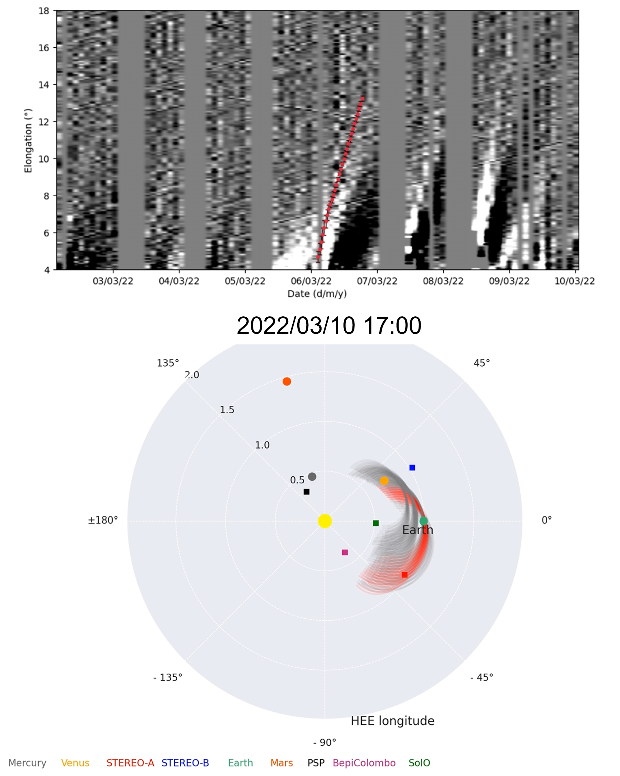
After observing the first event in Solar Orbiter at 2022-03-07 22:49 (case 1), we then tracked the CME front in the time-elongation maps generated from STEREO-A HI beacon data, from 6 March onwards. Following the method of \citeABauer2021, this procedure was repeated four more times and interpolated to an equally spaced time axis. This produced a single profile, as seen in the upper panel of Fig. 2, that was input into the ELEvoHI model to simulate the CME propagation towards Earth.
As discussed in Section 2.2, an ensemble of 210 model runs are used to make the final prediction of arrival time, as shown in lower panel of Fig. 2. The difference between the simulated and true arrival times over the ensemble are shown in Fig. 3, ranging from -7.8 hours to 47.1 hours (negative values indicate the prediction was earlier than the true arrival time). The mean error (ME) in arrival time at Earth was +8.1 hours, with a mean absolute error (MAE) of 10.4 hours (Table 1), representing typical values for such a simulation [Bauer \BOthers. (\APACyear2021), Amerstorfer \BOthers. (\APACyear2021)].
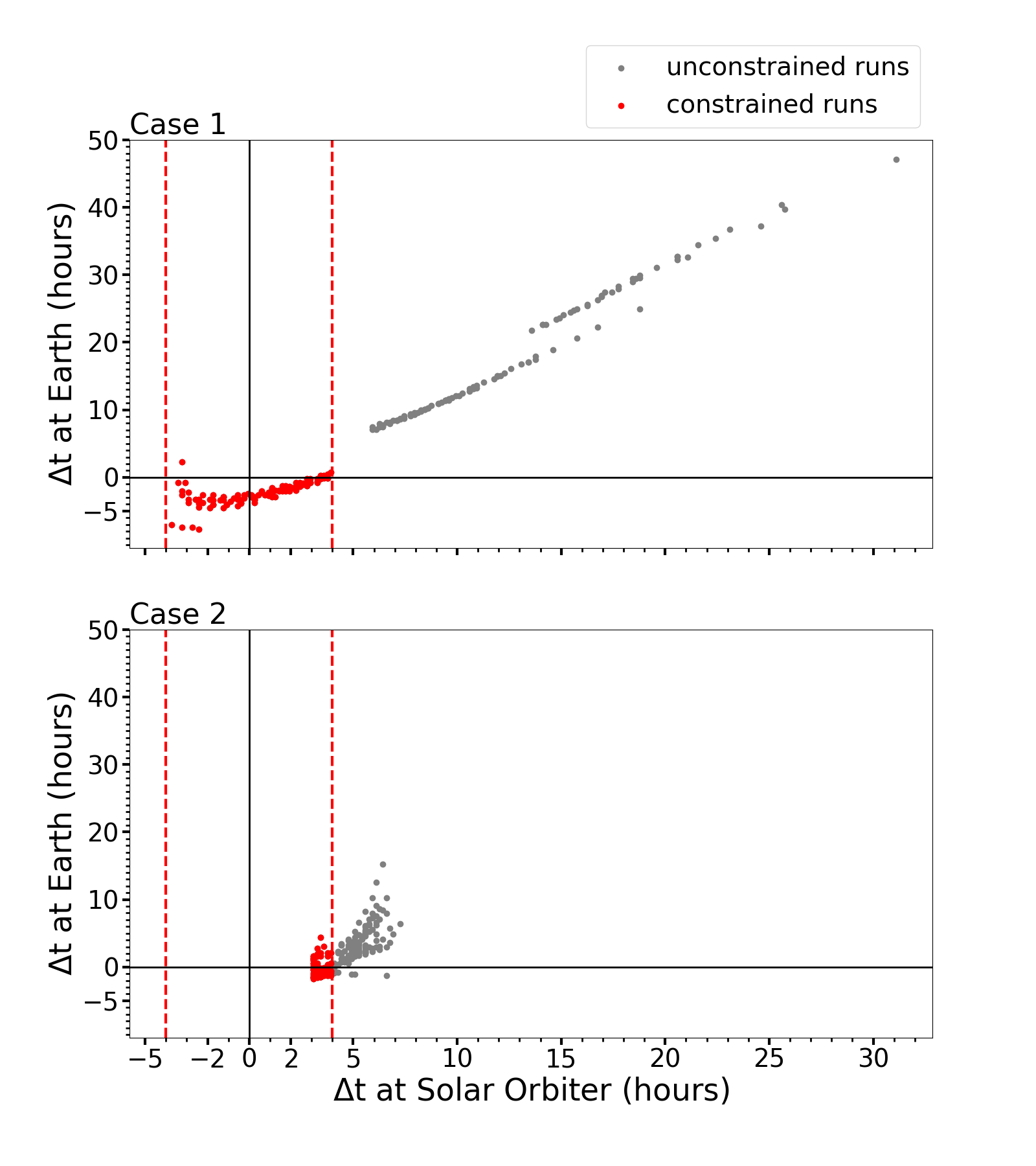
Using the arrival time at Solar Orbiter as a constraint, with a hour threshold, we were able to reject 111 of 210 ensemble members, leaving only 99 runs (red) in Figs. 2 and 3. This significantly improved the accuracy and precision of the simulation, lowering the ME to -2.4 hours and the MAE to 2.5 hours. In addition, by removing many of the erroneous runs, the range of arrival times was now between -7.7 hours to -2.3 hours. While constraining simulations in this way has been attempted in previous studies [Kubicka \BOthers. (\APACyear2016), Amerstorfer \BOthers. (\APACyear2018)], we have shown, for the first time, that this can lead to a drastically improved prediction in real time.
This same method was also applied to case 2, where the ME was reduced from +2.2 hours to -0.1 hours and the MAE improved from 2.7 hours to 1.1 hours. Although this was not done in real time, but still based on HI beacon data, it provided another successful demonstration of the benefits of constraining the ensemble runs. Such an improvement in arrival time was achieved even when the Solar Orbiter spacecraft was away from the Sun-Earth line. While this is only one example, it does suggest that a constellation of orbiting probes can be separated by at least 19∘ at 0.5 AU and still provide useful prediction capabilities.
Even without a complex model, but only using an estimated speed from PAS, we were still able to produce accurate arrival time predictions (Table 1). This is likely due to the fact that CMEs are relatively unaffected between 0.5 AU to AU, with any significant deflections having already mainly occurred closer to the Sun [Savani \BOthers. (\APACyear2010), Gui \BOthers. (\APACyear2011)]. Of course, CMEs are still known to deflect and deform in the solar wind depending on the downstream conditions [Owens (\APACyear2020), Desai \BOthers. (\APACyear2020), Hinterreiter, Amerstorfer, Reiss\BCBL \BOthers. (\APACyear2021), Davies \BOthers. (\APACyear2021)]. Such a problem could be addressed in future with an improved ELEvoHI model [Hinterreiter, Amerstorfer, Temmer\BCBL \BOthers. (\APACyear2021)], or with a 1D model that can capture CME deformation [Owens, Lang\BCBL \BOthers. (\APACyear2020)].
3.2 Magnetic field structure
Knowledge of the upstream CME conditions, namely proton speed, density and , is arguably of equal importance as the arrival time [Owens, Lockwood\BCBL \BBA Barnard (\APACyear2020)]. Such parameters influence the dynamic pressure of the CME and its ability to trigger magnetic reconnection at the magnetopause [Vasyliunas \BOthers. (\APACyear1982)], which leads to the onset of geomagnetic storms. The orientation of the magnetic field in the CME, whether is positive or negative, is the primary indicator of storm severity [Vasyliunas \BOthers. (\APACyear1982), Tsurutani \BOthers. (\APACyear1988), Gonzalez \BOthers. (\APACyear1999)], although predicting this property remains a challenging problem for CME models [Savani \BOthers. (\APACyear2015), Kay \BOthers. (\APACyear2017), Reiss \BOthers. (\APACyear2021)]. Therefore, it would be a major advantage if the transient structures seen by a spacecraft within AU were correlated with those subsequently seen at Earth.
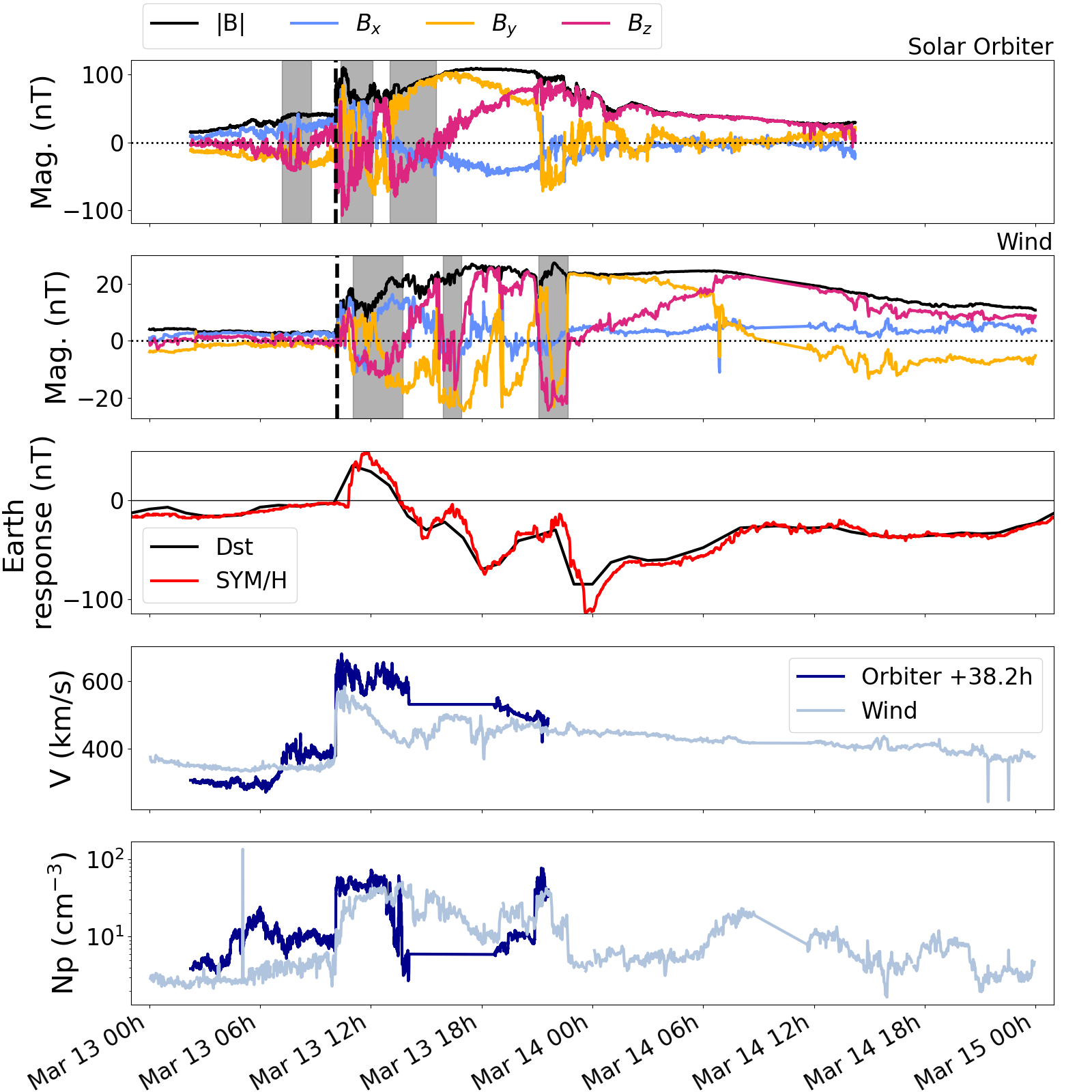
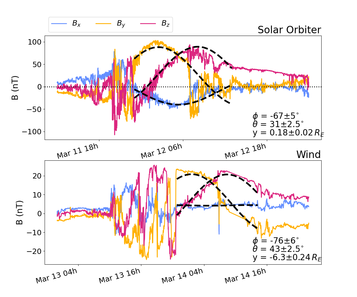
To evaluate the similarity in structure between the spacecraft, Fig. 4 shows the in situ measurements for case 2 from both Solar Orbiter and Wind, with the former time shifted to match up the shock fronts. Both spacecraft depict a typical CME profile, with a shock front occurring before a denser, more variable sheath region that was followed by the smooth rotation of the magnetic field in the flux rope. There was an excellent agreement in the profile between the two spacecraft, with three periods of negative (highlighted regions) followed by a flux rope with a mainly northward orientation. As expected, the first region in Solar Orbiter is now part of the CME sheath at Wind, having been overtaken by the shock. The profile was relatively unchanged at Wind due to the low inclination of the shock at Solar Orbiter, which had an azimuth () of and an elevation () of found using the cross product of the magnetic field either side of the shock111RTN coordinate system, where is the angle in the R-T plane where points along and along . is the angle out of the R-T plane..
Similarly, the signature was comparable in the CME flux rope between the two spacecraft, although, this was less clear for the other magnetic field components shown in Fig. 5. To further assess the similarity between the two CMEs, we fit the flux rope signatures with a simple force-free model assuming cylindrical symmetry and using Bessel function solutions [Burlaga (\APACyear1988), Lepping \BOthers. (\APACyear1990)]. We find a helicity sign of -1 for both events, and an azimuth, elevation and impact factor of (, , (0.8%)) for Solar Orbiter and (, , (19%)) for Wind. While the fitting is sensitive to variations in CME boundary definition, the results are consistent enough to demonstrate that the orientation of the flux rope remains fairly stable, with the changes in magnetic field component being mostly due to a change in impact factor. Such a scenario is consistent with the relative positions of the two spacecraft, with Solar Orbiter being away from the Sun-Earth line at 0.5 AU.
Therefore, both the orientation of the CME sheath and flux rope were similar between the spacecraft, demonstrating that CME structures can remain coherent between an upstream monitor and Earth. Interestingly, the magnetic response at Earth (Dst and SYM/H indices) was consistent with the signature at Solar Orbiter, displaying three dips before the flux rope slowly rotated northward. So, at least for this event, the magnetic storm indicators at Earth were strongly correlated to the magnetic structure seen at 0.5 AU around 40 hours prior. This suggests that with an upstream spacecraft, it is possible to predict not only the arrival of a CME, but the sub-structure of the flux rope and sheath region using measurements from 0.5 AU.
For this case, the magnetic field at Solar Orbiter was sufficient to capture the general trends in Dst at Earth, although, there were still some clear differences in Fig. 4. Much like the improvements in arrival time from Section 3.1, knowledge of the in situ CME properties, such as shock or flux rope orientation, could be used as the initial parameters for a CME propagation model [Sarkar \BOthers. (\APACyear2020)]. Again, this would not have to account for deflections in the corona, and should make for more accurate predictions of magnetic structure compared to those based on coronagraph observations. This would be another step towards being able to predict how the geomagnetic storm at Earth will develop on an hourly timescale.
It is important to note that this is only a single CME event, and a more extensive statistical study is needed. Indeed, the in situ structure of case 1 was a complex interaction of two flux ropes, rather than the typical sheath, flux rope profile seen in case 2. Nevertheless, the ability to predict CME structure is still extremely challenging for current models [Marubashi (\APACyear2000), Thernisien \BOthers. (\APACyear2009), Kay \BOthers. (\APACyear2017)], especially within the sheath region, which are known to be major drivers of geomagnetic storms [Tsurutani \BOthers. (\APACyear1988), Gonzalez \BOthers. (\APACyear1999), Lugaz \BOthers. (\APACyear2016)]. In future, given knowledge of the shock orientation at 0.5 AU, the Rankine-Hugoniot conditions could be applied to the ambient solar wind along the CME path to simulate the growth of the sheath region [Kay \BOthers. (\APACyear2022)].
4 Conclusions
In this study, we took advantage of an opportunity to use Solar Orbiter as an upstream space weather monitor between February and March 2022. As Solar Orbiter crossed the Sun-Earth line, we were able to use in situ data taken only 12 minutes earlier. In combination with the favourable position of STEREO-A, we were able to model the kinematics of two CME events with the ELEvoHI model.
We first demonstrated how knowledge of arrival time at Solar Orbiter could be used to constrain the ELEvoHI model. Under normal operation, this model uses an average of 210 ensemble members to estimate the arrival time of a CME at Earth. However, by only keeping those ensemble members that were within hours of the arrival time at Solar Orbiter, we improved both the accuracy and precision of the model. Specifically, the MAE was reduced from 10.4 hours to 2.5 hours and 2.7 hours to 1.1 hours in the two case studies. Therefore, for the first time, a numerical model was constrained with data from 0.5 AU to produce an updated prediction before the actual arrival of the CME at Earth. As well as demonstrating how a spacecraft at 0.5 AU could provide a lead time of over 40 hours, we also showed that the predictions were still accurate when Solar Orbiter was away from the Sun-Earth line. Such a result provides motivation for a future constellation mission housing in situ instrumentation, since the individual spacecraft could be separated by at least , making the concept more viable. While we could have used another CME model, we found it particularly beneficial to model the CMEs with the aid of STEREO-A HI data away the Sun-Earth line. Similar dedicated real time HI data can hopefully be provided by ESA’s Vigil mission in the near future.
We also found that even simple estimates of arrival time, using just the average CME speed at Solar Orbiter, could produce accurate arrival times at Earth. This represents a major benefit of an upstream solar wind monitor, as it reduces the need to model complex interactions and deflections in the corona, that can drastically alter arrival time. Of course, there is still a need to account for compression, distortion and rotation as the CME propagates in the solar wind. This, and the interaction between CMEs, could be handled by a 1D model [Owens, Lang\BCBL \BOthers. (\APACyear2020)] or an improved version of ELEvoHI in the future [Hinterreiter, Amerstorfer, Temmer\BCBL \BOthers. (\APACyear2021)].
Comparing measurements from Solar Orbiter and Wind revealed that the magnetic structure of the CME sheath and flux rope was remarkably similar for the second case study, despite being separated by 0.5 AU. Crucially, these periods of negative were also seen to match well with the magnetic response at Earth (Dst and SYM/H profiles), opening up the possibility to predict the evolution of a geomagnetic storm from measurements at 0.5 AU. This would also be important for reducing the number of false positive predictions, since the geo-effectiveness could be evaluated more than a day in advance.
In future, we hope that more models can make use of this data, either to constrain the output or to initiate a CME simulation away from the complex environment near the Sun. Fortunately, the opportunity to use Solar Orbiter for this purpose repeats once a year, with more CMEs being released as the Sun approaches solar maximum.
Open Research Section
The data used in this paper are available at the following places: Solar Orbiter data can be found on the Solar Orbiter archive (https://soar.esac.esa.int/soar/); Wind data can be found on CDAWeb (https://cdaweb.gsfc.nasa.gov/); quick look Dst data is available from https://wdc.kugi.kyoto-u.ac.jp/dst_realtime/index.html; the SYM/H data is available from https://wdc.kugi.kyoto-u.ac.jp/aeasy/ and STEREO/HI data are available from https://www.ukssdc.ac.uk/solar/stereo/data.html.
The ELEvoHI model is available on GitHub (https://github.com/tamerstorfer/ELEvoHI/releases/tag/v1.0.0.0).
Acknowledgements.
RL was supported by an Imperial College President’s Scholarship and TSH by STFC ST/S000364/1. The Solar Orbiter magnetometer was funded by the UK Space Agency (grant ST/T001062/1). We acknowledge the work of all the engineers who supported the instrument development and calibration, together with the engineering and technical staff at the European Space Agency, including all the Solar Orbiter instrument teams, and Airbus Space. T.A and M.B thank the Austrian Science Fund (FWF): P 36093, P31659. C.M. and E. E. D. are funded by the European Union (ERC, HELIO4CAST, 101042188). The HI instruments on STEREO were developed by a consortium that comprised the Rutherford Appleton Laboratory (UK), the University of Birmingham (UK), Centre Spatial de Liège (CSL, Belgium) and the Naval Research Laboratory (NRL, USA). The STEREO/SECCHI project, of which HI is a part, is an international consortium led by NRL. J.D., R.H and D.B. recognise the support of the UK Space Agency for funding STEREO/HI operations in the UK. M.D. acknowledges the support by the Croatian Science Foundation under the project IP-2020-02-9893 (ICOHOSS). Views and opinions expressed are however those of the author(s) only and do not necessarily reflect those of the European Union or the European Research Council Executive Agency. Neither the European Union nor the granting authority can be held responsible for them.References
- Amerstorfer \BOthers. (\APACyear2021) \APACinsertmetastarAmerstorfer2021{APACrefauthors}Amerstorfer, T., Hinterreiter, J., Reiss, M\BPBIA., Möstl, C., Davies, J\BPBIA., Bailey, R\BPBIL.\BDBLHarrison, R\BPBIA. \APACrefYearMonthDay2021. \BBOQ\APACrefatitleEvaluation of CME Arrival Prediction Using Ensemble Modeling Based on Heliospheric Imaging Observations Evaluation of CME Arrival Prediction Using Ensemble Modeling Based on Heliospheric Imaging Observations.\BBCQ \APACjournalVolNumPagesSpace Weather191e2020SW002553. {APACrefDOI} 10.1029/2020SW002553 \PrintBackRefs\CurrentBib
- Amerstorfer \BOthers. (\APACyear2018) \APACinsertmetastarAmerstorfer2018{APACrefauthors}Amerstorfer, T., Möstl, C., Hess, P., Temmer, M., Mays, M\BPBIL., Reiss, M\BPBIA.\BDBLBourdin, P\BHBIA. \APACrefYearMonthDay2018. \BBOQ\APACrefatitleEnsemble Prediction of a Halo Coronal Mass Ejection Using Heliospheric Imagers Ensemble Prediction of a Halo Coronal Mass Ejection Using Heliospheric Imagers.\BBCQ \APACjournalVolNumPagesSpace Weather167784–801. {APACrefDOI} 10.1029/2017SW001786 \PrintBackRefs\CurrentBib
- Angelini \BOthers. (\APACyear2022) \APACinsertmetastarAngelini2022{APACrefauthors}Angelini, V., O’Brien, H., Horbury, T.\BCBL \BBA Fauchon-Jones, E. \APACrefYearMonthDay2022\APACmonth05. \BBOQ\APACrefatitleNovel Magnetic Cleaning Techniques for Solar Orbiter Magnetometer Novel magnetic cleaning techniques for Solar Orbiter magnetometer.\BBCQ \BIn \APACrefbtitle2022 ESA Workshop on Aerospace EMC (Aerospace EMC) 2022 ESA Workshop on Aerospace EMC (Aerospace EMC) (\BPGS 1–6). {APACrefDOI} 10.23919/AerospaceEMC54301.2022.9828828 \PrintBackRefs\CurrentBib
- Auchère \BOthers. (\APACyear2020) \APACinsertmetastarAuchere2020{APACrefauthors}Auchère, F., Andretta, V., Antonucci, E., Bach, N., Battaglia, M., Bemporad, A.\BDBLZouganelis, I. \APACrefYearMonthDay2020\APACmonth10. \BBOQ\APACrefatitleCoordination within the Remote Sensing Payload on the Solar Orbiter Mission Coordination within the remote sensing payload on the Solar Orbiter mission.\BBCQ \APACjournalVolNumPagesAstronomy & Astrophysics642A6. {APACrefDOI} 10.1051/0004-6361/201937032 \PrintBackRefs\CurrentBib
- Bauer \BOthers. (\APACyear2021) \APACinsertmetastarBauer2021{APACrefauthors}Bauer, M., Amerstorfer, T., Hinterreiter, J., Weiss, A\BPBIJ., Davies, J\BPBIA., Möstl, C.\BDBLHarrison, R\BPBIA. \APACrefYearMonthDay2021. \BBOQ\APACrefatitlePredicting CMEs Using ELEvoHI With STEREO-HI Beacon Data Predicting CMEs Using ELEvoHI With STEREO-HI Beacon Data.\BBCQ \APACjournalVolNumPagesSpace Weather1912e2021SW002873. {APACrefDOI} 10.1029/2021SW002873 \PrintBackRefs\CurrentBib
- Burlaga (\APACyear1988) \APACinsertmetastarBurlaga1988{APACrefauthors}Burlaga, L\BPBIF. \APACrefYearMonthDay1988\APACmonth07. \BBOQ\APACrefatitleMagnetic Clouds and Force-Free Fields with Constant Alpha Magnetic clouds and force-free fields with constant alpha.\BBCQ \APACjournalVolNumPagesJournal of Geophysical Research937217–7224. {APACrefDOI} 10.1029/JA093iA07p07217 \PrintBackRefs\CurrentBib
- Davies \BOthers. (\APACyear2021) \APACinsertmetastarDavies2021a{APACrefauthors}Davies, E\BPBIE., Möstl, C., Owens, M\BPBIJ., Weiss, A\BPBIJ., Amerstorfer, T., Hinterreiter, J.\BDBLHarrison, R\BPBIA. \APACrefYearMonthDay2021\APACmonth12. \BBOQ\APACrefatitleIn Situ Multi-Spacecraft and Remote Imaging Observations of the First CME Detected by Solar Orbiter and BepiColombo In situ multi-spacecraft and remote imaging observations of the first CME detected by Solar Orbiter and BepiColombo.\BBCQ \APACjournalVolNumPagesAstronomy & Astrophysics656A2. {APACrefDOI} 10.1051/0004-6361/202040113 \PrintBackRefs\CurrentBib
- Desai \BOthers. (\APACyear2020) \APACinsertmetastarDesai2020{APACrefauthors}Desai, R\BPBIT., Zhang, H., Davies, E\BPBIE., Stawarz, J\BPBIE., Mico-Gomez, J.\BCBL \BBA Iváñez-Ballesteros, P. \APACrefYearMonthDay2020\APACmonth09. \BBOQ\APACrefatitleThree-Dimensional Simulations of Solar Wind Preconditioning and the 23 July 2012 Interplanetary Coronal Mass Ejection Three-Dimensional Simulations of Solar Wind Preconditioning and the 23 July 2012 Interplanetary Coronal Mass Ejection.\BBCQ \APACjournalVolNumPagesSolar Physics2959130. {APACrefDOI} 10.1007/s11207-020-01700-5 \PrintBackRefs\CurrentBib
- Eastwood, Biffis\BCBL \BOthers. (\APACyear2017) \APACinsertmetastarEastwood2017a{APACrefauthors}Eastwood, J\BPBIP., Biffis, E., Hapgood, M\BPBIA., Green, L., Bisi, M\BPBIM., Bentley, R\BPBID.\BDBLBurnett, C. \APACrefYearMonthDay2017. \BBOQ\APACrefatitleThe Economic Impact of Space Weather: Where Do We Stand? The Economic Impact of Space Weather: Where Do We Stand?\BBCQ \APACjournalVolNumPagesRisk Analysis372. {APACrefDOI} 10.1111/risa.12765 \PrintBackRefs\CurrentBib
- Eastwood, Nakamura\BCBL \BOthers. (\APACyear2017) \APACinsertmetastarEastwood2017{APACrefauthors}Eastwood, J\BPBIP., Nakamura, R., Turc, L., Mejnertsen, L.\BCBL \BBA Hesse, M. \APACrefYearMonthDay2017\APACmonth11. \BBOQ\APACrefatitleThe Scientific Foundations of Forecasting Magnetospheric Space Weather The Scientific Foundations of Forecasting Magnetospheric Space Weather.\BBCQ \APACjournalVolNumPagesSpace Science Reviews2123-41221–1252. {APACrefDOI} 10.1007/s11214-017-0399-8 \PrintBackRefs\CurrentBib
- Eyles \BOthers. (\APACyear2009) \APACinsertmetastarEyles2009{APACrefauthors}Eyles, C\BPBIJ., Harrison, R\BPBIA., Davis, C\BPBIJ., Waltham, N\BPBIR., Shaughnessy, B\BPBIM., Mapson-Menard, H\BPBIC\BPBIA.\BDBLRochus, P. \APACrefYearMonthDay2009\APACmonth02. \BBOQ\APACrefatitleThe Heliospheric Imagers Onboard the STEREO Mission The Heliospheric Imagers Onboard the STEREO Mission.\BBCQ \APACjournalVolNumPagesSolar Physics2542387–445. {APACrefDOI} 10.1007/s11207-008-9299-0 \PrintBackRefs\CurrentBib
- Gonzalez \BOthers. (\APACyear1999) \APACinsertmetastarGonzalez1999{APACrefauthors}Gonzalez, W\BPBID., Tsurutani, B\BPBIT.\BCBL \BBA Clúa de Gonzalez, A\BPBIL. \APACrefYearMonthDay1999\APACmonth04. \BBOQ\APACrefatitleInterplanetary Origin of Geomagnetic Storms Interplanetary origin of geomagnetic storms.\BBCQ \APACjournalVolNumPagesSpace Science Reviews883529–562. {APACrefDOI} 10.1023/A:1005160129098 \PrintBackRefs\CurrentBib
- Good \BOthers. (\APACyear2019) \APACinsertmetastarGood2019{APACrefauthors}Good, S\BPBIW., Kilpua, E\BPBIK\BPBIJ., LaMoury, A\BPBIT., Forsyth, R\BPBIJ., Eastwood, J\BPBIP.\BCBL \BBA Möstl, C. \APACrefYearMonthDay2019. \BBOQ\APACrefatitleSelf-Similarity of ICME Flux Ropes: Observations by Radially Aligned Spacecraft in the Inner Heliosphere Self-Similarity of ICME Flux Ropes: Observations by Radially Aligned Spacecraft in the Inner Heliosphere.\BBCQ \APACjournalVolNumPagesJournal of Geophysical Research: Space Physics12474960–4982. {APACrefDOI} 10.1029/2019JA026475 \PrintBackRefs\CurrentBib
- Gui \BOthers. (\APACyear2011) \APACinsertmetastarGui2011{APACrefauthors}Gui, B., Shen, C., Wang, Y., Ye, P., Liu, J., Wang, S.\BCBL \BBA Zhao, X. \APACrefYearMonthDay2011\APACmonth07. \BBOQ\APACrefatitleQuantitative Analysis of CME Deflections in the Corona Quantitative Analysis of CME Deflections in the Corona.\BBCQ \APACjournalVolNumPagesSolar Physics2711111–139. {APACrefDOI} 10.1007/s11207-011-9791-9 \PrintBackRefs\CurrentBib
- Hapgood (\APACyear2012) \APACinsertmetastarHapgood2012{APACrefauthors}Hapgood, M. \APACrefYearMonthDay2012\APACmonth04. \BBOQ\APACrefatitlePrepare for the Coming Space Weather Storm Prepare for the coming space weather storm.\BBCQ \APACjournalVolNumPagesNature4847394311–313. {APACrefDOI} 10.1038/484311a \PrintBackRefs\CurrentBib
- Heiligers \BBA McInnes (\APACyear2014) \APACinsertmetastarHeiligers2014{APACrefauthors}Heiligers, J.\BCBT \BBA McInnes, C. \APACrefYearMonthDay2014\APACmonth01. \BBOQ\APACrefatitleNovel Solar Sail Mission Concepts for Space Weather Forecasting Novel solar sail mission concepts for Space weather forecasting.\BBCQ \BIn \APACrefbtitle24th AAS/AIAA Space Flight Mechanics Meeting 2014 24th AAS/AIAA Space Flight Mechanics Meeting 2014 (\BPGS AAS 14–239). \PrintBackRefs\CurrentBib
- Hinterreiter, Amerstorfer, Reiss\BCBL \BOthers. (\APACyear2021) \APACinsertmetastarHinterreiter2021a{APACrefauthors}Hinterreiter, J., Amerstorfer, T., Reiss, M\BPBIA., Möstl, C., Temmer, M., Bauer, M.\BDBLOwens, M\BPBIJ. \APACrefYearMonthDay2021. \BBOQ\APACrefatitleWhy Are ELEvoHI CME Arrival Predictions Different If Based on STEREO-A or STEREO-B Heliospheric Imager Observations? Why are ELEvoHI CME Arrival Predictions Different if Based on STEREO-A or STEREO-B Heliospheric Imager Observations?\BBCQ \APACjournalVolNumPagesSpace Weather193e2020SW002674. {APACrefDOI} 10.1029/2020SW002674 \PrintBackRefs\CurrentBib
- Hinterreiter, Amerstorfer, Temmer\BCBL \BOthers. (\APACyear2021) \APACinsertmetastarHinterreiter2021{APACrefauthors}Hinterreiter, J., Amerstorfer, T., Temmer, M., Reiss, M\BPBIA., Weiss, A\BPBIJ., Möstl, C.\BDBLAmerstorfer, U\BPBIV. \APACrefYearMonthDay2021. \BBOQ\APACrefatitleDrag-Based CME Modeling With Heliospheric Images Incorporating Frontal Deformation: ELEvoHI 2.0 Drag-Based CME Modeling With Heliospheric Images Incorporating Frontal Deformation: ELEvoHI 2.0.\BBCQ \APACjournalVolNumPagesSpace Weather1910e2021SW002836. {APACrefDOI} 10.1029/2021SW002836 \PrintBackRefs\CurrentBib
- Horbury \BOthers. (\APACyear2020) \APACinsertmetastarHorbury2020a{APACrefauthors}Horbury, T\BPBIS., O’Brien, H., Carrasco Blazquez, I., Bendyk, M., Brown, P., Hudson, R.\BDBLWalsh, A\BPBIP. \APACrefYearMonthDay2020. \BBOQ\APACrefatitleThe Solar Orbiter Magnetometer The Solar Orbiter magnetometer.\BBCQ \APACjournalVolNumPagesA&A642A9. {APACrefDOI} 10.1051/0004-6361/201937257 \PrintBackRefs\CurrentBib
- Kay \BOthers. (\APACyear2017) \APACinsertmetastarKay2017{APACrefauthors}Kay, C., Gopalswamy, N., Reinard, A.\BCBL \BBA Opher, M. \APACrefYearMonthDay2017\APACmonth01. \BBOQ\APACrefatitlePredicting the Magnetic Field of Earth-impacting CMEs Predicting the Magnetic Field of Earth-impacting CMEs.\BBCQ \APACjournalVolNumPagesThe Astrophysical Journal8352117. {APACrefDOI} 10.3847/1538-4357/835/2/117 \PrintBackRefs\CurrentBib
- Kay \BOthers. (\APACyear2022) \APACinsertmetastarKay2022{APACrefauthors}Kay, C., Nieves-Chinchilla, T., Hofmeister, S\BPBIJ.\BCBL \BBA Palmerio, E. \APACrefYearMonthDay2022. \BBOQ\APACrefatitleBeyond Basic Drag in Interplanetary CME Modeling: Effects of Solar Wind Pileup and High-Speed Streams Beyond Basic Drag in Interplanetary CME Modeling: Effects of Solar Wind Pileup and High-Speed Streams.\BBCQ \APACjournalVolNumPagesSpace Weather209e2022SW003165. {APACrefDOI} 10.1029/2022SW003165 \PrintBackRefs\CurrentBib
- Kubicka \BOthers. (\APACyear2016) \APACinsertmetastarKubicka2016{APACrefauthors}Kubicka, M., Möstl, C., Amerstorfer, T., Boakes, P\BPBID., Feng, L., Eastwood, J\BPBIP.\BCBL \BBA Törmänen, O. \APACrefYearMonthDay2016\APACmonth12. \BBOQ\APACrefatitlePREDICTION OF GEOMAGNETIC STORM STRENGTH FROM INNER HELIOSPHERIC IN SITU OBSERVATIONS PREDICTION OF GEOMAGNETIC STORM STRENGTH FROM INNER HELIOSPHERIC IN SITU OBSERVATIONS.\BBCQ \APACjournalVolNumPagesThe Astrophysical Journal8332255. {APACrefDOI} 10.3847/1538-4357/833/2/255 \PrintBackRefs\CurrentBib
- Lepping \BOthers. (\APACyear1990) \APACinsertmetastarLepping1990{APACrefauthors}Lepping, R\BPBIP., Jones, J\BPBIA.\BCBL \BBA Burlaga, L\BPBIF. \APACrefYearMonthDay1990\APACmonth08. \BBOQ\APACrefatitleMagnetic Field Structure of Interplanetary Magnetic Clouds at 1 AU Magnetic field structure of interplanetary magnetic clouds at 1 AU.\BBCQ \APACjournalVolNumPagesJournal of Geophysical Research9511957–11965. {APACrefDOI} 10.1029/JA095iA08p11957 \PrintBackRefs\CurrentBib
- Lindsay \BOthers. (\APACyear1999) \APACinsertmetastarLindsay1999{APACrefauthors}Lindsay, G\BPBIM., Russell, C\BPBIT.\BCBL \BBA Luhmann, J\BPBIG. \APACrefYearMonthDay1999\APACmonth05. \BBOQ\APACrefatitlePredictability of Dst Index Based upon Solar Wind Conditions Monitored inside 1 AU Predictability of Dst index based upon solar wind conditions monitored inside 1 AU.\BBCQ \APACjournalVolNumPagesJournal of Geophysical Research: Space Physics104A510335–10344. {APACrefDOI} 10.1029/1999JA900010 \PrintBackRefs\CurrentBib
- Lugaz \BOthers. (\APACyear2016) \APACinsertmetastarLugaz2016{APACrefauthors}Lugaz, N., Farrugia, C\BPBIJ., Winslow, R\BPBIM., Al-Haddad, N., Kilpua, E\BPBIK\BPBIJ.\BCBL \BBA Riley, P. \APACrefYearMonthDay2016. \BBOQ\APACrefatitleFactors Affecting the Geoeffectiveness of Shocks and Sheaths at 1 AU Factors affecting the geoeffectiveness of shocks and sheaths at 1 AU.\BBCQ \APACjournalVolNumPagesJournal of Geophysical Research: Space Physics1211110,861–10,879. {APACrefDOI} 10.1002/2016JA023100 \PrintBackRefs\CurrentBib
- Marubashi (\APACyear2000) \APACinsertmetastarMarubashi2000{APACrefauthors}Marubashi, K. \APACrefYearMonthDay2000\APACmonth01. \BBOQ\APACrefatitlePhysics of Interplanetary Magnetic Flux Ropes: Toward Prediction of Geomagnetic Storms Physics of interplanetary magnetic flux ropes: Toward prediction of geomagnetic storms.\BBCQ \APACjournalVolNumPagesAdvances in Space Research26155–66. {APACrefDOI} 10.1016/S0273-1177(99)01026-1 \PrintBackRefs\CurrentBib
- Möstl \BOthers. (\APACyear2015) \APACinsertmetastarMostl2015{APACrefauthors}Möstl, C., Rollett, T., Frahm, R\BPBIA., Liu, Y\BPBID., Long, D\BPBIM., Colaninno, R\BPBIC.\BDBLVršnak, B. \APACrefYearMonthDay2015\APACmonth05. \BBOQ\APACrefatitleStrong Coronal Channelling and Interplanetary Evolution of a Solar Storm up to Earth and Mars Strong coronal channelling and interplanetary evolution of a solar storm up to Earth and Mars.\BBCQ \APACjournalVolNumPagesNature Communications617135. {APACrefDOI} 10.1038/ncomms8135 \PrintBackRefs\CurrentBib
- Müller \BOthers. (\APACyear2020) \APACinsertmetastarMuller2020{APACrefauthors}Müller, D., Cyr, O\BPBIC\BPBIS., Zouganelis, I., Gilbert, H\BPBIR., Marsden, R., Nieves-Chinchilla, T.\BDBLWilliams, D. \APACrefYearMonthDay2020\APACmonth10. \BBOQ\APACrefatitleThe Solar Orbiter Mission - Science Overview The Solar Orbiter mission - Science overview.\BBCQ \APACjournalVolNumPagesAstronomy & Astrophysics642A1. {APACrefDOI} 10.1051/0004-6361/202038467 \PrintBackRefs\CurrentBib
- Owen \BOthers. (\APACyear2020) \APACinsertmetastarOwen2020{APACrefauthors}Owen, C\BPBIJ., Bruno, R., Livi, S., Louarn, P., Al Janabi, K., Allegrini, F.\BDBLZouganelis, I. \APACrefYearMonthDay2020. \BBOQ\APACrefatitleThe Solar Orbiter Solar Wind Analyser (SWA) Suite The Solar Orbiter Solar Wind Analyser (SWA) suite.\BBCQ \APACjournalVolNumPagesA&A642A16. {APACrefDOI} 10.1051/0004-6361/201937259 \PrintBackRefs\CurrentBib
- Owens (\APACyear2020) \APACinsertmetastarOwens2020c{APACrefauthors}Owens, M\BPBIJ. \APACrefYearMonthDay2020. \BBOQ\APACrefatitleCoherence of Coronal Mass Ejections in Near-Earth Space Coherence of Coronal Mass Ejections in Near-Earth Space.\BBCQ \APACjournalVolNumPagesSolar Physics295101–13. {APACrefDOI} 10.1007/s11207-020-01721-0 \PrintBackRefs\CurrentBib
- Owens, Lang\BCBL \BOthers. (\APACyear2020) \APACinsertmetastarOwens2020d{APACrefauthors}Owens, M\BPBIJ., Lang, M., Barnard, L., Riley, P., Ben-Nun, M., Scott, C\BPBIJ.\BDBLGonzi, S. \APACrefYearMonthDay2020\APACmonth03. \BBOQ\APACrefatitleA Computationally Efficient, Time-Dependent Model of the Solar Wind for Use as a Surrogate to Three-Dimensional Numerical Magnetohydrodynamic Simulations A Computationally Efficient, Time-Dependent Model of the Solar Wind for Use as a Surrogate to Three-Dimensional Numerical Magnetohydrodynamic Simulations.\BBCQ \APACjournalVolNumPagesSolar Physics295343. {APACrefDOI} 10.1007/s11207-020-01605-3 \PrintBackRefs\CurrentBib
- Owens, Lockwood\BCBL \BBA Barnard (\APACyear2020) \APACinsertmetastarOwens2020e{APACrefauthors}Owens, M\BPBIJ., Lockwood, M.\BCBL \BBA Barnard, L\BPBIA. \APACrefYearMonthDay2020\APACmonth09. \BBOQ\APACrefatitleThe Value of CME Arrival Time Forecasts for Space Weather Mitigation The Value of CME Arrival Time Forecasts for Space Weather Mitigation.\BBCQ \APACjournalVolNumPagesSpace Weather189e2020SW002507. {APACrefDOI} 10.1029/2020SW002507 \PrintBackRefs\CurrentBib
- Reiss \BOthers. (\APACyear2021) \APACinsertmetastarReiss2021{APACrefauthors}Reiss, M\BPBIA., Möstl, C., Bailey, R\BPBIL., Rüdisser, H\BPBIT., Amerstorfer, U\BPBIV., Amerstorfer, T.\BDBLWindisch, A. \APACrefYearMonthDay2021\APACmonth12. \BBOQ\APACrefatitleMachine Learning for Predicting the Bz Magnetic Field Component From Upstream in Situ Observations of Solar Coronal Mass Ejections Machine Learning for Predicting the Bz Magnetic Field Component From Upstream in Situ Observations of Solar Coronal Mass Ejections.\BBCQ \APACjournalVolNumPagesSpace Weather19e2021SW002859. {APACrefDOI} 10.1029/2021SW002859 \PrintBackRefs\CurrentBib
- Richardson \BOthers. (\APACyear2001) \APACinsertmetastarRichardson2001{APACrefauthors}Richardson, I\BPBIG., Cliver, E\BPBIW.\BCBL \BBA Cane, H\BPBIV. \APACrefYearMonthDay2001\APACmonth07. \BBOQ\APACrefatitleSources of Geomagnetic Storms for Solar Minimum and Maximum Conditions during 1972–2000 Sources of geomagnetic storms for solar minimum and maximum conditions during 1972–2000.\BBCQ \APACjournalVolNumPagesGeophysical Research Letters28132569–2572. {APACrefDOI} 10.1029/2001GL013052 \PrintBackRefs\CurrentBib
- Riley \BOthers. (\APACyear2018) \APACinsertmetastarRiley2018{APACrefauthors}Riley, P., Mays, M\BPBIL., Andries, J., Amerstorfer, T., Biesecker, D., Delouille, V.\BDBLZhao, X. \APACrefYearMonthDay2018. \BBOQ\APACrefatitleForecasting the Arrival Time of Coronal Mass Ejections: Analysis of the CCMC CME Scoreboard Forecasting the Arrival Time of Coronal Mass Ejections: Analysis of the CCMC CME Scoreboard.\BBCQ \APACjournalVolNumPagesSpace Weather1691245–1260. {APACrefDOI} 10.1029/2018SW001962 \PrintBackRefs\CurrentBib
- Rollett \BOthers. (\APACyear2016) \APACinsertmetastarRollett2016{APACrefauthors}Rollett, T., Möstl, C., Isavnin, A., Davies, J\BPBIA., Kubicka, M., Amerstorfer, U\BPBIV.\BCBL \BBA Harrison, R\BPBIA. \APACrefYearMonthDay2016\APACmonth06. \BBOQ\APACrefatitleElEvoHI: A NOVEL CME PREDICTION TOOL FOR HELIOSPHERIC IMAGING COMBINING AN ELLIPTICAL FRONT WITH DRAG-BASED MODEL FITTING ElEvoHI: A NOVEL CME PREDICTION TOOL FOR HELIOSPHERIC IMAGING COMBINING AN ELLIPTICAL FRONT WITH DRAG-BASED MODEL FITTING.\BBCQ \APACjournalVolNumPagesThe Astrophysical Journal8242131. {APACrefDOI} 10.3847/0004-637X/824/2/131 \PrintBackRefs\CurrentBib
- Rollett \BOthers. (\APACyear2014) \APACinsertmetastarRollett2014{APACrefauthors}Rollett, T., Möstl, C., Temmer, M., Frahm, R\BPBIA., Davies, J\BPBIA., Veronig, A\BPBIM.\BDBLZhang, T\BPBIL. \APACrefYearMonthDay2014\APACmonth07. \BBOQ\APACrefatitleCombined Multipoint Remote and in Situ Observations of the Asymmetric Evolution of a Fast Solar Coronal Mass Ejection Combined Multipoint Remote and in situ Observations of the Asymmetric Evolution of a Fast Solar Coronal Mass Ejection.\BBCQ \APACjournalVolNumPagesThe Astrophysical Journal790L6. {APACrefDOI} 10.1088/2041-8205/790/1/L6 \PrintBackRefs\CurrentBib
- Sarkar \BOthers. (\APACyear2020) \APACinsertmetastarSarkar2020{APACrefauthors}Sarkar, R., Gopalswamy, N.\BCBL \BBA Srivastava, N. \APACrefYearMonthDay2020\APACmonth01. \BBOQ\APACrefatitleAn Observationally Constrained Analytical Model for Predicting the Magnetic Field Vectors of Interplanetary Coronal Mass Ejections at 1 Au An Observationally Constrained Analytical Model for Predicting the Magnetic Field Vectors of Interplanetary Coronal Mass Ejections at 1 au.\BBCQ \APACjournalVolNumPagesThe Astrophysical Journal8882121. {APACrefDOI} 10.3847/1538-4357/ab5fd7 \PrintBackRefs\CurrentBib
- Savani \BOthers. (\APACyear2010) \APACinsertmetastarSavani2010{APACrefauthors}Savani, N\BPBIP., Owens, M\BPBIJ., Rouillard, A\BPBIP., Forsyth, R\BPBIJ.\BCBL \BBA Davies, J\BPBIA. \APACrefYearMonthDay2010\APACmonth04. \BBOQ\APACrefatitleOBSERVATIONAL EVIDENCE OF A CORONAL MASS EJECTION DISTORTION DIRECTLY ATTRIBUTABLE TO A STRUCTURED SOLAR WIND OBSERVATIONAL EVIDENCE OF A CORONAL MASS EJECTION DISTORTION DIRECTLY ATTRIBUTABLE TO A STRUCTURED SOLAR WIND.\BBCQ \APACjournalVolNumPagesThe Astrophysical Journal Letters7141L128. {APACrefDOI} 10.1088/2041-8205/714/1/L128 \PrintBackRefs\CurrentBib
- Savani \BOthers. (\APACyear2015) \APACinsertmetastarSavani2015{APACrefauthors}Savani, N\BPBIP., Vourlidas, A., Szabo, A., Mays, M\BPBIL., Richardson, I\BPBIG., Thompson, B\BPBIJ.\BDBLNieves-Chinchilla, T. \APACrefYearMonthDay2015. \BBOQ\APACrefatitlePredicting the Magnetic Vectors within Coronal Mass Ejections Arriving at Earth: 1. Initial Architecture Predicting the magnetic vectors within coronal mass ejections arriving at Earth: 1. Initial architecture.\BBCQ \APACjournalVolNumPagesSpace Weather136374–385. {APACrefDOI} 10.1002/2015SW001171 \PrintBackRefs\CurrentBib
- Sheeley \BOthers. (\APACyear1999) \APACinsertmetastarSheeley1999{APACrefauthors}Sheeley, N\BPBIR., Walters, J\BPBIH., Wang, Y\BPBIM.\BCBL \BBA Howard, R\BPBIA. \APACrefYearMonthDay1999\APACmonth11. \BBOQ\APACrefatitleContinuous Tracking of Coronal Outflows: Two Kinds of Coronal Mass Ejections Continuous tracking of coronal outflows: Two kinds of coronal mass ejections.\BBCQ \APACjournalVolNumPagesJournal of Geophysical Research10424739–24768. {APACrefDOI} 10.1029/1999JA900308 \PrintBackRefs\CurrentBib
- Thernisien \BOthers. (\APACyear2009) \APACinsertmetastarThernisien2009{APACrefauthors}Thernisien, A., Vourlidas, A.\BCBL \BBA Howard, R\BPBIA. \APACrefYearMonthDay2009\APACmonth05. \BBOQ\APACrefatitleForward Modeling of Coronal Mass Ejections Using STEREO/SECCHI Data Forward Modeling of Coronal Mass Ejections Using STEREO/SECCHI Data.\BBCQ \APACjournalVolNumPagesSolar Physics2561111–130. {APACrefDOI} 10.1007/s11207-009-9346-5 \PrintBackRefs\CurrentBib
- Tsurutani \BOthers. (\APACyear1988) \APACinsertmetastarTsurutani1988{APACrefauthors}Tsurutani, B\BPBIT., Gonzalez, W\BPBID., Tang, F., Akasofu, S\BPBII.\BCBL \BBA Smith, E\BPBIJ. \APACrefYearMonthDay1988\APACmonth08. \BBOQ\APACrefatitleOrigin of Interplanetary Southward Magnetic Fields Responsible for Major Magnetic Storms near Solar Maximum (1978-1979) Origin of interplanetary southward magnetic fields responsible for major magnetic storms near solar maximum (1978-1979).\BBCQ \APACjournalVolNumPagesJournal of Geophysical Research938519–8531. {APACrefDOI} 10.1029/JA093iA08p08519 \PrintBackRefs\CurrentBib
- Vasyliunas \BOthers. (\APACyear1982) \APACinsertmetastarVasyliunas1982{APACrefauthors}Vasyliunas, V\BPBIM., Kan, J\BPBIR., Siscoe, G\BPBIL.\BCBL \BBA Akasofu, S\BPBII. \APACrefYearMonthDay1982\APACmonth04. \BBOQ\APACrefatitleScaling Relations Governing Magnetospheric Energy Transfer Scaling relations governing magnetospheric energy transfer.\BBCQ \APACjournalVolNumPagesPlanetary and Space Science304359–365. {APACrefDOI} 10.1016/0032-0633(82)90041-1 \PrintBackRefs\CurrentBib
- Verbeke \BOthers. (\APACyear2019) \APACinsertmetastarVerbeke2019{APACrefauthors}Verbeke, C., Mays, M\BPBIL., Temmer, M., Bingham, S., Steenburgh, R., Dumbović, M.\BDBLAndries, J. \APACrefYearMonthDay2019\APACmonth01. \BBOQ\APACrefatitleBenchmarking CME Arrival Time and Impact: Progress on Metadata, Metrics, and Events Benchmarking CME Arrival Time and Impact: Progress on Metadata, Metrics, and Events.\BBCQ \APACjournalVolNumPagesSpace Weather1716–26. {APACrefDOI} 10.1029/2018SW002046 \PrintBackRefs\CurrentBib
- Vršnak \BOthers. (\APACyear2013) \APACinsertmetastarVrsnak2013{APACrefauthors}Vršnak, B., Žic, T., Vrbanec, D., Temmer, M., Rollett, T., Möstl, C.\BDBLShanmugaraju, A. \APACrefYearMonthDay2013\APACmonth07. \BBOQ\APACrefatitlePropagation of Interplanetary Coronal Mass Ejections: The Drag-Based Model Propagation of Interplanetary Coronal Mass Ejections: The Drag-Based Model.\BBCQ \APACjournalVolNumPagesSolar Physics2851295–315. {APACrefDOI} 10.1007/s11207-012-0035-4 \PrintBackRefs\CurrentBib
- Wang \BOthers. (\APACyear2004) \APACinsertmetastarWang2004{APACrefauthors}Wang, Y., Shen, C., Wang, S.\BCBL \BBA Ye, P. \APACrefYearMonthDay2004\APACmonth08. \BBOQ\APACrefatitleDeflection of Coronal Mass Ejection in the Interplanetary Medium Deflection of coronal mass ejection in the interplanetary medium.\BBCQ \APACjournalVolNumPagesSolar Physics2222329–343. {APACrefDOI} 10.1023/B:SOLA.0000043576.21942.aa \PrintBackRefs\CurrentBib
- Wang \BOthers. (\APACyear2002) \APACinsertmetastarWang2002{APACrefauthors}Wang, Y., Wang, S.\BCBL \BBA Ye, P. \APACrefYearMonthDay2002\APACmonth12. \BBOQ\APACrefatitleMultiple Magnetic Clouds in Interplanetary Space Multiple magnetic clouds in interplanetary space.\BBCQ \APACjournalVolNumPagesSolar Physics2111333–344. {APACrefDOI} 10.1023/A:1022404425398 \PrintBackRefs\CurrentBib
- Wold \BOthers. (\APACyear2018) \APACinsertmetastarWold2018{APACrefauthors}Wold, A\BPBIM., Mays, M\BPBIL., Taktakishvili, A., Jian, L\BPBIK., Odstrcil, D.\BCBL \BBA MacNeice, P. \APACrefYearMonthDay2018. \BBOQ\APACrefatitleVerification of Real-Time WSA-ENLIL+Cone Simulations of CME Arrival-Time at the CCMC from 2010 to 2016 Verification of real-time WSA-ENLIL+Cone simulations of CME arrival-time at the CCMC from 2010 to 2016.\BBCQ \APACjournalVolNumPagesJournal of Space Weather and Space Climate8A17. {APACrefDOI} 10.1051/swsc/2018005 \PrintBackRefs\CurrentBib