Waveform and Beamforming Optimization for Wireless Power Transfer with Dynamic Metasurface Antennas

Abstract

Radio frequency (RF) wireless power transfer (WPT) is a promising charging technology for future wireless systems. However, low end-to-end power transfer efficiency (PTE) is a critical challenge for practical implementations. One of the main inefficiency sources is the power consumption and loss of key components such as the high-power amplifier (HPA) and rectenna, which must be considered for PTE optimization. Herein, we investigate the power consumption of an RF-WPT system considering the emerging dynamic metasurface antenna (DMA) as the transmitter. Moreover, we incorporate the HPA and rectenna non-linearities and consider the Doherty HPA to reduce power consumption. We provide a mathematical framework to calculate each user’s harvested power from multi-tone signal transmissions and the system power consumption. Then, the waveform and beamforming are designed using swarm-based intelligence to minimize power consumption while satisfying the users’ energy harvesting (EH) requirements. Numerical results manifest that increasing the number of transmit tones enhances the performance in terms of coverage probability and power consumption since the HPAs operate below the saturation region in the simulation setup and the EH non-linearity is the dominant factor. Finally, our findings demonstrate that a properly shaped DMA may outperform a fully-digital antenna of the same size.

I Introduction

Future wireless systems will facilitate efficient and environmentally-friendly communication across a myriad of low-power devices, thus promoting a sustainable society. To achieve this vision, it is imperative to enable seamless and uninterrupted connectivity among these devices, as well as with the underlying infrastructure, all while mitigating disruptions arising from battery depletion [1, 2]. This is potentially facilitated by energy harvesting (EH) technologies providing wireless charging capability without physical contact, thus easing the maintenance of Internet of Things (IoT) devices and increasing their operational lifetime. Moreover, EH may lead to improved energy efficiency and reduced emission footprints across the network [3].

EH receivers may harvest energy from two types of sources: those that exist in the surrounding environment, and those that are specifically designated for energy transmission. From a transmission perspective, the latter is supported by wireless power transfer (WPT) technologies, e.g., based on inductive coupling, magnetic resonance coupling, laser power beaming, and radio frequency (RF) radiation. Among them, using RF radiation, a.k.a. RF-WPT, is promising for charging multiple users relatively far from the power sources by exploiting the broadcast nature of wireless channels. Furthermore, this can be accomplished over the same infrastructure used for wireless communication. Notably, the most important challenge toward maturing the RF-WPT technology is related to increasing the inherently low end-to-end power transfer efficiency (PTE) [3]. Herein, we focus on RF-WPT, which is referred to as WPT in the following.

The end-to-end PTE of a WPT system depends mainly on the performance of its key building blocks, namely energy transmitter (ET), wireless channel, and energy receiver (ER) as illustrated in Fig. 1. At first, a signal is generated and amplified using a DC power source at the ET. Then, it is upconverted to the RF domain and transmitted over the wireless channel. Finally, the ER converts the received RF signal to DC for EH purposes.

Figure 1: Block diagram of a typical WPT system. The power consumption and loss sources are listed under each block.

Indeed, the end-to-end PTE comprises: DC-to-RF, RF-to-RF, and RF-to-DC power conversion efficiency, i.e.,

$$e=\underbrace{\frac{P^{t}_{rf}}{P^{t}_{dc}}}_{e_{1}}\times\underbrace{\frac{P^{r}_{rf}}{P^{t}_{rf}}}_{e_{2}}\times\underbrace{\frac{P^{r}_{dc}}{P^{r}_{rf}}}_{e_{3}}=\frac{P^{r}_{dc}}{P^{t}_{dc}}.$$ (1)

In a WPT system, both transmitter and receiver introduce non-linearities that affect the signal. Indeed, an appropriately designed and amplified transmit signal leveraging these non-linearities might reduce the power consumption at the transmitter and/or increase the RF-to-DC conversion efficiency at the receiver [4, 5]. More precisely, using multiple transmit frequency tones can lead to high peak-to-average power ratio (PAPR) signals at the receiver, which enhances the rectifier RF-to-DC conversion efficiency [6, 7, 8]. Meanwhile, the RF signal can be focused towards the ER using energy beamforming (EB), which affects the transmit/receive waveform, to cope with the channel inefficiencies captured by $e_{2}$, thereby enhancing the amount of RF power that can be harvested [3]. Moreover, notice that the active transmit components consume power to operate, while the passive elements introduce power losses, both of which impact $e_{1}$ and must be considered. Therefore, $e_{1}$, $e_{2}$, and $e_{3}$ are correlated, which suggests that their joint optimization may lead to significant gains in terms of end-to-end PTE.

There are many works either focusing on EB optimization, e.g., [9, 10, 11], or waveform optimization, e.g., [12, 13, 14], while much less on their joint optimization, e.g., [15, 16]. Moreover, the practical non-linearities of a WPT system are not considered in [9, 11], while the frameworks in [12, 13, 15, 10, 16] considered the rectifier non-linearity, but not the transmit HPA non-linearity. Interestingly, the authors in [14] consider both rectifier and HPA non-linearities. Therein, the amount of harvested power is maximized by optimizing a multi-carrier waveform and investigating its influence on the system’s non-linearities.

One of the main factors contributing greatly to the system power consumption is the architecture of the transmitter, which also determines the beamforming approach. For example, in a fully-digital architecture, each transmitting antenna necessitates a dedicated RF chain, with its corresponding HPA, consuming a significant amount of power. An HPA aims to amplify the input signal to compensate for the path loss and fading in a wireless system. Moreover, the signal amplification in the HPA requires a DC power source, which accounts for the majority of the power consumption. Notably, the HPA introduces non-linear signal distortion that requires precise modeling [17, 18]. The significant drawback of the fully-digital architecture is the high complexity and cost, making it impractical for applications requiring massive MIMO (mMIMO) implementations. Alternatively, analog architectures using, e.g., passive phase shifters, are less expensive but offer limited degrees of freedom for EB. Thus, a hybrid architecture implementation combining both approaches is often more appealing in practice. Hybrid architectures offer a trade-off between complexity (cost) and beamforming flexibility [19, 20].

Although analog beamforming promotes cost reduction, it still requires complex analog networks for phase shifting. Indeed, there are emerging technologies to provide beamforming capability with an even lower cost and complexity, e.g. intelligent reflecting surface (IRS)-aided systems [21] and dynamic metasurface antennas (DMAs) [22]. Notice that IRS is an assisting node that provides the passive beamforming capability using reflective elements, while DMA is a transceiver consisting of configurable metamaterial elements and a limited number of RF chains. Furthermore, one key challenge regarding IRS-aided systems is acquiring the channel state information (CSI) [23]. Indeed, the passive beamforming gain highly depends on accurate CSI while the IRS lacks the baseband processing capability to perform channel estimation and send pilot signals. Meanwhile, DMA avoids analog network implementation challenges and provides beamforming capability with low cost and complexity. Also, CSI acquisition is not a big issue since DMA is a transceiver and has enough baseband processing capability for channel estimation. Notably, DMA is utilized in [24, 25] for a near-field WPT system without considering the HPA and rectifier non-linearities. Additionally, the joint waveform and beamforming design problem in IRS-aided WPT and simultaneous wireless information and power transfer systems is investigated in [16, 26], respectively. Furthermore, these works consider the EH non-linearity but not the transmit HPA. Notice that the elements of the IRS are just reflective elements causing phase shifts, while the operation of the DMA elements is constrained and cannot be simply modeled like an ideal phase shifter [27].

All in all, WPT systems have received considerable attention for some time. Still, we consider that more effort is needed to reduce the system power consumption, thus increasing the end-to-end PTE. For this, low-cost multi-antenna transmitters like DMA are appealing and may pave the way for charging devices efficiently in massive IoT deployments. Moreover, although multiple studies aimed to enhance the harvested power in WPT systems, no work has yet investigated the power consumption of a multi-antenna WPT system while considering the main non-linearity and power consumption sources. Herein, we aim precisely to fill this research gap. Our main contributions are as follows:

1) We formulate a joint waveform and beamforming design problem for a multi-user multi-antenna WPT system with both a fully-digital and a DMA architecture transmitting signals over a near-field wireless channel, which can inherently capture far-field conditions as well. In contrast to the previous works [16, 14], which focused on increasing the amount of harvested power, we aim to minimize the power consumption of the system while meeting the EH requirements of the users. Notice that this formulation mimics a practical setup where the EH users inform their energy demands and the WPT system must serve them with minimum power consumption, thus maximum end-to-end PTE. Since the HPA is an active element incurring most of the power consumption at the transmitter side, we adopt the high-efficiency 2-way Doherty HPA to further reduce the power consumption of the system. Notably, our problem shares some similarities with the one discussed in [14] as objectives and constraints are interchanged. However, we deal with an additional non-linearity due to the power consumption model of the Doherty HPA, while our considered DMA-assisted architecture makes the beamforming problem considerably more complex by incorporating metamaterial elements with a Lorentzian-constrained phase response. Note that the metamaterial elements phase shifts are not ideal, which results in a different beamforming problem than other architectures, e.g., IRS-assisted systems [26] and hybrid beamforming [20]. The complexities associated with our specific problem make the existing optimization frameworks for WPT systems inapplicable to our system, which calls for a novel solution to address them.

2) We propose a two-stage optimization approach based on particle swarm optimization (PSO) for the joint waveform and beamforming design. Specifically, we include the users’ harvesting DC power requirements constraints in the objective function of the optimization problem, compelling the algorithm to discover a feasible solution before minimizing the power consumption. By this means, we cope with the non-convex nature and extensive non-linearities of the problem, introduced by the HPA input-output relation, the HPA power consumption model, the phase model of the metamaterial elements, and the EH model. Furthermore, the complexity of the proposed algorithm scales linearly with the number of users, antenna elements, frequency tones, time samples, and the PSO algorithm parameters.

3) We show numerically that HPAs operate below the saturation region in our simulation setup, thus, increasing the number of transmit tones can enhance the coverage probability and reduce the power consumption of the system by leveraging the rectifier non-linearity. Furthermore, we show that the DMA outperforms the fully-digital setup when the number of sub-carriers and array size are relatively small. Meanwhile, the results indicate that the fully-digital architecture may perform better when the number of tones is sufficiently large, but with much higher complexity and number of RF chains. Finally, we discuss the role of the Doherty HPA in the achieved system performance and provide evidence that the HPA efficiency is much higher in the DMA-assisted system because of the lower number of RF chains compared to the fully-digital setup.

The remainder of the paper is structured as follows. Section II introduces the system model, including the transmit architectures and channel model. Section III provides the signal and power consumption modeling throughout the system while discussing the HPA and rectenna non-linearities. The formulation of the optimization problem for a joint waveform and beamforming design, together with the proposed solving approach, are elaborated in Section IV. Section V presents the numerical results and related discussions, while Section VI concludes the paper.

We adopt the following notations. Bold lower-case and upper-case letters represent column vectors and matrices, respectively. Non-boldface characters refer to scalars, ${\mathbf{a}}\odot{\mathbf{b}}$ denotes the Hadamard product of $\mathbf{a}$ and $\mathbf{b}$, and $\{x\}$ is a set that contains $x$. The $l_{2}$-norm of a vector is denoted as $|\cdot|$. The mathematical expectation is represented by $\mathbb{E}$ and $(\cdot)^{T}$ is used to indicate the transpose of a matrix or vector. Furthermore, the real and the imaginary parts of a complex number are denoted by $\Re\{\cdot\}$ and $\Im\{\cdot\}$, respectively. Additionally, $\lfloor{\cdot}\rfloor$ is the floor operator and $\mathbbm{1}{(\cdot)}$ is the indicator function.

II System Model

We consider a multi-antenna WPT system to charge $M$ single-antenna EH devices over a period of time. The received RF power at the EH device is transferred into the rectifier input using a matching network. Then, it is converted to DC power using the rectifier for EH purposes. The EH requirement of each device is denoted by $\tilde{P}_{dc}$.

As previously mentioned, multi-tone waveforms can be exploited to leverage the rectifier and HPA non-linearities and achieve a better end-to-end PTE. Hence, we consider multi-tone signals with $N_{f}$ tones at frequencies $f_{1},f_{2},\cdots,f_{N_{f}}$ for power transmission purposes. Without loss of generality, one can set

$$f_{n}=f_{1}+(n-1)\Delta_{f},$$ (2)

where $f_{1}$, $\Delta_{f}=\frac{\mathrm{BW}}{N_{f}}$, and $\mathrm{BW}$ are the lowest sub-carrier frequency, the sub-carrier spacing, and the system bandwidth, respectively.

The rest of this section describes the transmit architectures and the channel model.

II-A Transmit Antenna Architectures

The transmitter is equipped with a uniform planar array (UPA) and $N_{rf}$ RF chains. The radiating elements are spaced uniformly, with $N_{h}$ and $N_{v}$ being the number of elements in the horizontal and vertical direction, respectively. Thus, the total number of elements is $N=N_{v}\times N_{h}$.

Two types of transmit antenna architectures are considered:

1) Fully-digital architecture, which requires a dedicated RF chain for each radiating element, thus $N_{rf}=N$, as shown in Fig. 2a. In a fully-digital architecture, there is a single-stage beamforming process. Herein, we define $\mathbf{W}\in\mathbb{C}^{N_{rf}\times N_{f}}$ as the digital precoding matrix, such that $\mathbf{W}=\begin{bmatrix}\mathbf{w}_{1},\mathbf{w}_{2},\ldots,\mathbf{w}_{N_{rf}}\end{bmatrix}^{T}$, and $\mathbf{w}_{k}=[\omega_{k,1},\omega_{k,2},\ldots,\omega_{k,N_{f}}]^{T}$ is the vector containing the complex weights of the $k$th muti-tone waveform. Despite the high deployment cost and complexity, a fully-digital structure offers the highest number of degrees of freedom in beamforming.

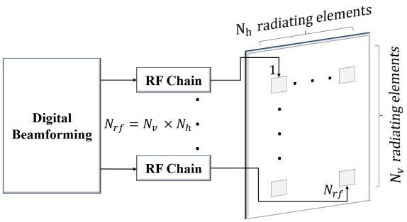
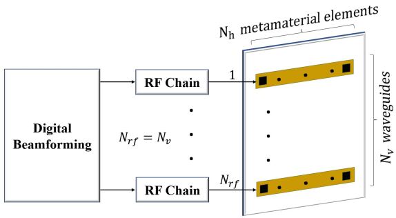
Figure 2: Transmit antenna architectures. (a) Fully-digital architecture (left) and (b) DMA-based architecture (right).

2) DMA-assisted architecture, which comprises $N_{v}$ waveguides, each fed by a dedicated RF chain and composed by $N_{h}$ configurable metamaterial elements. Therefore, the number of RF chains, and consequently the cost and complexity, is considerably reduced with respect to digital architectures, making DMA-assisted architectures suitable for mMIMO applications. Notice that DMA-assisted systems employ a two-stage beamforming process, i.e., digital beamforming, followed by the tuning of the amplitude/phase variations introduced by the metamaterial elements. Herein, $\mathbf{W}\in\mathbb{C}^{N_{rf}\times N_{f}}$ is the digital precoding matrix and $\mathbf{Q}=\begin{bmatrix}\boldsymbol{\phi}_{1},\boldsymbol{\phi}_{2},\ldots,\boldsymbol{\phi}_{N_{v}}\end{bmatrix}^{T}\in\mathbb{C}^{N_{v}\times N_{h}}$ is the matrix containing the phases configured in the metamaterial elements, where $\boldsymbol{\phi}_{i}=[\phi_{i,1},\phi_{i,2},\ldots,\phi_{i,N_{h}}]^{T}$. Moreover, $\phi_{i,l}\in[0,2\pi]$ is the phase of the $l$th metamaterial element in the $i$th waveguide.

II-B Channel Model

In wireless communications, the region where the users are located between the Fraunhofer and Fresnel distances, denoted respectively as $d$ and $d^{\prime}$, is referred to as the near-field region. Specifically, a device at distance $r_{m}$ from a transmitter experiences near-field conditions if

$$\sqrt[3]{\frac{D^{4}}{8\lambda}}=d<r_{m}<d^{\prime}=\frac{2D^{2}}{\lambda},$$ (3)

where $D$ is the antenna diameter, i.e., the largest size of the antenna aperture, and $\lambda$ is the wavelength. Notice that both system frequency and antenna form factor influence the region of operation. Therefore, by moving toward higher frequencies, e.g., millimeter wave and sub-THz bands, and utilizing larger antenna arrays, the far-field communication assumption regarding planar wavefronts may not be valid anymore. Instead, wavefronts impinging a receive node may be strictly spherical, thus, with advanced capabilities to focus the transmit signals on specific spatial points rather on spatial directions.

Indoor environments with line of sight and near-field communication are particularly relevant for many WPT applications, especially when utilizing large antenna arrays and operating at high frequencies. Thus, we employ the near-field channel model described in [28]. The Cartesian coordinate of the $l$th radiating element in the $i$th row is $\mathbf{g}_{i,l}=[x_{i,l},y_{i,l},z_{i,l}]^{T}$. Additionally, $i=1,2,\ldots,N_{v}$ and $l=1,2,\ldots,N_{h}$. The channel coefficient between user $m$ and the $l$th element in the $i$th row at the $n$th sub-carrier is given by

$$\gamma_{i,l,m,n}=A_{i,l,m,n}e^{\frac{-j2\pi}{\lambda_{n}}d_{i,l,m}},$$ (4)

where ${\frac{2\pi}{\lambda_{n}}d_{i,l,m}}$ is the phase shift caused by the propagation distance of the $n$th tone, with wavelength $\lambda_{n}$, from the transmitter to the receiver and $d_{i,l,m}=|\mathbf{g}_{m}-\mathbf{g}_{i,l}|$ is the Euclidean distance between the element and the user located at $\mathbf{g}_{m}$. Moreover,

$$A_{i,l,m,n}=\sqrt{F(\Theta_{i,l,m})}\frac{\lambda_{n}}{4\pi d_{i,l,m}}$$ (5)

is the corresponding channel gain coefficient. Here, $\Theta_{i,l,m}=(\theta_{i,l,m},\psi_{i,l,m})$ is the elevation-azimuth angle pair, and $F(\Theta_{i,l,m})$ is the radiation profile of each element. In addition, we employ the radiation profile formulation as presented in [29], where

$$F(\Theta_{i,l,m})=\begin{cases}G_{t}\cos{(\theta_{i,l,m})}^{\frac{G_{t}}{2}-1},&\theta_{i,l,m}\in[0,\pi/2],\\ 0,&\text{otherwise},\end{cases}$$ (6)

$G_{t}=2(b+1)$ is the transmit antenna gain, and $b$ denotes the boresight gain, which depends on the specifications of the antenna elements. Note that the channel coefficient becomes $A_{m}e^{-j\psi_{i,l,m}}$ for far-field communication, where $A_{m}$ only depends on the distance of the user $m$ from the transmitter and $\psi_{i,l,m}$ is solely determined by the user direction and the relative disposition of the antenna elements within the array.

III Transceiver and Signal Modeling

This section discusses the signal model and relevant features of the transmit and receive nodes. The latter includes the non-linearities introduced by HPA and rectenna, and the power consumption of both fully-digital and DMA-based transmit architectures.

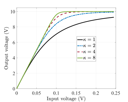
Figure 3: Rapp model for the input-output relation of an HPA with $G=20$ dB, $B_{s}=10$ V, and different $\kappa$ values.

III-A HPA

The signal at the input of the $k$th HPA is given by

$$x_{k}(t)=\sum_{n=1}^{N_{f}}{\omega_{k,n}e^{j2\pi f_{n}t}},\quad k=1,\ldots,N_{rf}.$$ (7)

Moreover, HPA introduces signal distortion and we use the Rapp model for solid-state power amplifiers [30] to model such non-linearity. Mathematically, the output signal of the HPA is modeled as

$$x^{hpa}_{k}(t)=\frac{Gx_{k}(t)}{G^{\prime}({x_{k}(t))}},$$ (8)

where $G^{\prime}({x_{k}(t)})=\Big{[}1+\big{(}\frac{G|x_{k}(t)|}{B_{s}}\big{)}^{2\kappa}\Big{]}^{1/(2\kappa)}$, and $\kappa$, $G$, and $B_{s}$ represent the smoothness factor, gain, and saturation voltage, respectively. Fig. 3 depicts the input-output characteristics of a particular HPA. It can be seen that the HPA operates linearly at low-power levels, whereas the non-linearity increases with input power until reaching the saturation level.

III-B Transmit & Receive Signals

The rest of the signal modeling formulation will be presented separately for fully-digital and DMA-based architecture in the following.

III-B1 Fully-Digital Architecture

Herein, $N_{rf}=N$, thus, the real transmit signal at the output of the $l$th element in the $i$th row of the UPA can be expressed as

$$\quad x^{FD}_{i,l}(t)=\Re\biggl{\{}x^{hpa}_{u{(i,l)}}(t)\biggr{\}}=\frac{G}{G^{\prime}({x_{u{(i,l)}}(t))}}\sum_{n=1}^{N_{f}}\Re\biggl{\{}\omega_{{u{(i,l)}},n}e^{j2\pi f_{n}t}\biggr{\}},$$ (9)

where ${u{(i,l)}}=(i-1)N_{h}+l$. Thereby, the RF signal at the $m$th receiver when exploiting the fully-digital architecture can be expressed as

$$y^{FD}_{m}(t)\!=\!\sum_{i=1}^{N_{v}}\sum_{l=1}^{N_{h}}\sum_{n=1}^{N_{f}}\gamma_{i,l,m,n}x^{FD}_{i,l}(t)\!=\!\frac{G}{G^{\prime}({x_{u{(i,l)}}(t))}}\sum_{i=1}^{N_{v}}\sum_{l=1}^{N_{h}}\sum_{n=1}^{N_{f}}\Re\Bigl{\{}\gamma_{i,l,m,n}\omega_{{u{(i,l)}},n}e^{j2\pi f_{n}t}\Bigr{\}}.$$ (10)

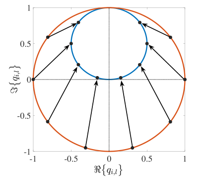
Figure 4: The Lorentzian constrained (the inner circle) and the ideal weights (outer circle) in the complex plane. The arrows depict the mapping between the weights.

III-B2 DMA-assisted Architecture

In metasurface antennas, the phase and amplitude that can be configured in the radiating elements are correlated due to the Lorentzian resonance. Herein, we capture this correlation by [27]

$$q_{i,l}=\frac{j+e^{j\phi_{i,l}}}{2},$$ (11)

where $q_{i,l}$ and $\phi_{i,l}$ are the tunable response and phase of the $l$th metamaterial element in the $i$th waveguide, respectively. As shown in Fig. 4, the ideal weights exhibit a constant unit amplitude, i.e., no losses, while the amplitude of the Lorentzian weights depends on the configured phase.

Herein, microstrip lines are used as waveguides, similar to [31, 28]. The propagation model of the signal within a microstrip is expressed as

$$h_{i,l}=e^{-(l-1)d_{l}(\alpha_{i}+j\beta_{i})},$$ (12)

where $d_{l}$ is the inter-element distance, $\alpha_{i}$ represents the waveguide attenuation coefficient, and $\beta_{i}$ is the propagation constant. The mathematical model of the DMA is represented in Fig. 5.

We know the number of RF chains in the DMA-assisted system is reduced to $N_{rf}=N_{v}$. Hence, by using (8), the real transmit signal radiated from the $l$th element in the $i$th microstrip can be expressed as

$$x_{i,l}^{DMA}(t)=\frac{G}{G^{\prime}({x_{i}(t)})}\Re\left\{h_{i,l}q_{i,l}x_{i}^{hpa}(t)\right\}.$$ (13)

Furthermore, the RF signal received by the $m$th user in the DMA-assisted system is given by

$$y^{DMA}_{m}(t)\!=\!\sum_{i=1}^{N_{v}}\!\sum_{l=1}^{N_{h}}\!\sum_{n=1}^{N_{f}}\gamma_{i,l,m,n}x_{i,l}^{DMA}(t)\!=\!\frac{G}{G^{\prime}({x_{i}(t)})}\sum_{i=1}^{N_{v}}\!\sum_{l=1}^{N_{h}}\!\sum_{n=1}^{N_{f}}\!\Re\Bigl{\{}\gamma_{i,l,m,n}h_{i,l}q_{i,l}\omega_{i,n}e^{j2\pi f_{n}t}\Bigr{\}}.$$ (14)

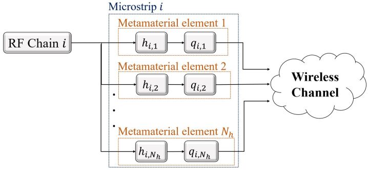
Figure 5: Mathematical model of the DMA.

III-C Rectenna

The RF signal is converted to DC at the receiver. This can be modeled by an antenna equivalent circuit and a single diode rectifier as illustrated in Fig. 6.

The RF signal at the input of the antenna is denoted as $y_{m}(t)$ and has an average power of $\mathbb{E}\bigl{\{}{y_{m}(t)}^{2}\bigr{\}}$. Let us denote the input impedance of the rectifier and the impedance of the antenna equivalent circuit by $R_{in}$ and $R_{ant}$, respectively. Thus, assuming perfect matching $(R_{in}=R_{ant})$, the input voltage at the rectifier of the $m$th ER is given by

$$v_{{in},{m}}(t)=y_{m}(t)\sqrt{R_{ant}}.$$ (15)

Furthermore, the diode current can be formulated as

$$i_{d}(t)=i_{s}\bigl{(}e^{\frac{v_{d}(t)}{n_{i}v_{t}}}-1\bigr{)},$$ (16)

where $i_{s}$ is the reverse bias saturation current, $n_{i}$ is the ideality factor, $v_{t}$ is the thermal voltage, and $v_{d}(t)=v_{in}(t)-v_{out}(t)$ is the diode voltage. Moreover, $v_{{out},{m}}(t)$ is the output voltage of the $m$th rectifier, which can be approximated utilizing the Taylor expansion, as [15, 13]

$$v_{{out},{m}}=\sum_{i\ even,i\geq 2}^{n_{0}}\beta_{i}\mathbb{E}\bigl{\{}y_{m}(t)^{i}\bigr{\}},$$ (17)

where $\beta_{i}=\frac{R_{ant}^{i/2}}{i!{(n_{i}v_{t})}^{i-1}}$. Herein, we focus on the low-power regime, for which it was demonstrated in [13, 32] that truncating the Taylor expansion at $n_{0}=4$ is accurate enough. Therefore, (17) can be written as

$$v_{{out},{m}}=\beta_{2}\mathbb{E}\bigl{\{}y_{m}(t)^{2}\bigr{\}}+\beta_{4}\mathbb{E}\bigl{\{}y_{m}(t)^{4}\bigr{\}}$$ (18)

and the DC power at the $m$th receiver is given by

$$P_{{dc},m}=\frac{{v_{{out},{m}}}^{2}}{R_{L}},$$ (19)

where $R_{L}$ is the load impedance of the rectifier circuit. Note that $y_{m}(t)$ is equal to $y_{m}^{DMA}(t)$ and $y_{m}^{FD}(t)$ in the DMA-based and fully-digital structure, respectively.

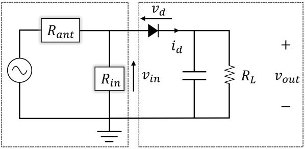
Figure 6: Antenna equivalent circuit (left) and a single diode rectifier (right) [15].

III-D Power Consumption Model

Lowering the power consumption is desirable for increasing the PTE and this greatly depends on the efficiency of the utilized HPA. Motivated by this, we utilize the high-efficiency Doherty HPA [33], where multiple HPAs are combined to operate in different output power ranges. Specifically, we adopt the $2$-way symmetric Doherty HPA described in [34], where the HPAs operate in class-B mode. Furthermore, we consider the maximum efficiency of the class-B HPA to be $\frac{\pi}{4}$. Then, the power consumption of the $k$th HPA at time $t$ can be written as

$$P_{{pa},k}(t)=\begin{cases}\frac{2}{\pi}\sqrt{P_{max}P_{{out},k}(t)},&0<P_{{out},k}(t)\leq\frac{1}{4}P_{max},\\ \frac{6}{\pi}\sqrt{P_{max}P_{{out},k}(t)}-\frac{2}{\pi}P_{max},&\frac{1}{4}P_{max}<P_{{out},k}(t)\leq P_{max},\end{cases}$$ (20)

where $P_{max}\propto{B_{s}}^{2}$ is the saturation power and $P_{{out},k}(t)\propto|x_{k}^{hpa}(t)|^{2}$ is the instantaneous output power of the $k$th HPA. Moreover, $x_{k}^{hpa}(t)$ can be calculated using (8), where the saturation level for $0<P_{{out},k}(t)\leq 0.25P_{max}$ and $0.25P_{max}<P_{{out},k}(t)\leq P_{max}$ are considered to be $0.25P_{max}$ and $P_{max}$, respectively. Note that, the power consumption of a single class-B HPA is given by $\frac{4}{\pi}\sqrt{P_{max}P_{out}}$. Fig. 7 compares the power consumption of the Doherty and class-B HPA based on the output power level. It is evident that the Doherty HPA consumes less power throughout the entire output power range that is below the saturation level. Furthermore, the HPA power consumption increases with its output. Therefore, the HPA efficiency, i.e.,

$$\varepsilon_{pa}=\frac{P_{out}}{P_{pa}+P_{in}},$$ (21)

is maximum when the HPA operates near the saturation region and $P_{in}$ is the input signal power. Meanwhile, the efficiency may decrease when the HPA enters this region because it cannot further increase the output power linearly with $P_{in}$.

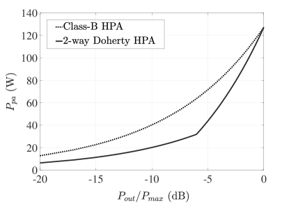
Figure 7: The power consumption of the HPAs with $G=20$ dB, $B_{s}=10$ V, and $\kappa=4$.

There are also other power consumption sources in the WPT system, which will be discussed in this section. Specifically, $P_{bb}$ denotes the digital baseband power consumption. This amount of power is required to perform the digital beamforming and the generation of digital precoding vectors. Furthermore, $P_{rf}$ represents the RF chain circuit power consumption, including the mixer, local oscillator, and filter. Thus, the total power consumption of the system is given by

$$P_{c}=P_{bb}+N_{rf}P_{rf}+\sum_{k=1}^{N_{rf}}\mathbb{E}\bigl{\{}P_{{pa},k}(t)\bigr{\}}+P_{{in},k},$$ (22)

where $P_{{in},k}=\sum_{n=1}^{N_{f}}|\omega_{k,n}|^{2}$ is the input power to the $k$th HPA. Recall that $N_{rf}$ is equal to $N$ and $N_{v}$ in a fully-digital and DMA-based structure, respectively. Finally, the end-to-end PTE of the system is given by

$$\mathrm{PTE}=\sum_{m=1}^{M}P_{{dc},m}/{P_{c}}.$$ (23)

IV Joint Waveform and Beamforming Optimization

This section formalizes the optimization problem and describes the utilized approach when employing the aforementioned transmit architectures.

IV-A Problem Formulation

The goal is to fulfill the EH requirements of the users while minimizing power consumption. Therefore, the optimization problem can be formulated as

$$\operatorname*{minimize}_{\mathbf{V}}\quad P_{c}$$ (24a)

subject to $$P_{{dc},m}\geq\tilde{P}_{dc},\quad\forall m\in\mathcal{M},$$ (24b)

where $P_{c}$ is the power consumption of the system, which was given in the previous section for each transmit architecture. Additionally, $\mathbf{V}$ is the beamforming matrix, which is equal to $\mathbf{W}\in\mathbb{C}^{N_{rf}\times N_{f}}$ for the fully-digital architecture and $\begin{bmatrix}\mathbf{W},\mathbf{Q}\end{bmatrix}$ for the DMA architecture.

The optimization problem in (24) deals with extensive non-linearity. Specifically, (24a) includes the term $\sum_{k=1}^{N_{rf}}\mathbb{E}\bigl{\{}P_{{pa},k}(t)\bigr{\}}$ which is a non-convex function of $\mathbf{V}$ and depends on the HPA non-linearity and power consumption model. Similarly, (24b) depends on metamaterial’s frequency response and the HPA and rectenna non-linearities. Notably, the authors in [14] focus on maximizing the harvested power, which solely addresses the numerator of (23). Thus, the optimal waveform design may result in high power consumption and low end-to-end PTE in that case. In contrast, our proposed formulation considers both the numerator and denominator of (23). As a result, it prevents excessive increases in power consumption and allows for adaptation to the desired harvested DC power of the users in practical WPT systems.

Considering a fully-digital architecture with a single class-B HPA in each RF chain, it has been proven in [14] that $v_{{out},m}$ is convex with respect to the transmit waveform. Furthermore, the authors handle the relation between the transmit and input waveforms through equality constraints. Then, they utilize successive convex programming to approximate the objective function (harvested DC power), and sequential quadratic programming to deal with the non-linear constraints of the problem. Thereby, they find an approximate solution for the harvested power maximization problem. Note that problem (24) introduces more complexity compared to the one in [14] due to the Doherty HPA model and the metamaterial elements phase response. Hence, the optimization variables in the DMA-assisted system are not just the digital beamforming weights (input waveform) anymore, and the metamaterial elements should be configured as well. Meanwhile, although the fully-digital architecture does not have the elements’ frequency response complexity, it still requires to cope with the additional complexity introduced by the Doherty HPA model. Specifically, (20) comprises two distinct regions, evincing the need to consider the operational regime of the HPA during the optimization procedure.

IV-B PSO Framework

PSO, initially proposed in [35], constitutes an evolutionary algorithm based on swarm intelligence that is suitable for identifying local optima in tangled problems, such as (24). In PSO, each potential solution in the problem space has two primary attributes: its position, i.e., the variables’ value, and the velocity. Moreover, the velocity determines the solution movement within the problem space, and by updating it at every iteration, the solutions gradually converge towards a local optimum for the objective function [36]. The readers may refer to [37] for more details on PSO.

Algorithm 1 PSO

Inputs: $\tilde{B}$, $\mathcal{S}$, $N_{var}$, $F$, $c_{1}$, $c_{2}$, $\eta$, $c_{max}$, $I_{max}$, ${\mathbf{z}_{min}}$, ${\mathbf{z}_{max}}$

Outputs: $\mathbf{z}_{r^{*}}$, ${B}^{*}$

Initialize:

     $\mathbf{p}_{r}=\mathbf{z}_{r},\ \forall r$

     $r^{*}=\operatorname*{argmin}_{r}{\xi\big{(}\Lambda(\mathbf{z}_{r})\big{)}}$

     $B^{*}=\xi\bigl{(}\Lambda(\mathbf{z}_{r^{*}})\bigr{)}$

     $N_{nb}=\max{(2,\lfloor|\mathcal{S}|\times\eta\rfloor)}$, $c_{s}=0$, $iter=1$

repeat

     for $r=1,\ldots,|\mathcal{S}|$ do

          Choose $\mathcal{K}\subset\mathcal{S}\backslash\mathbf{z}_{r}$ randomly, such that $|\mathcal{K}|=N_{nb}$

         $j^{*}=\operatorname*{argmin}_{j}{\xi\bigl{(}\Lambda(\mathbf{z}_{j})\bigr{)}},\ \mathbf{z}_{j}\in\mathcal{K}$

         Select $\mathbf{u}_{1}$ and $\mathbf{u}_{2}$ randomly in $(0,1)^{N_{var}\times 1}$

         $\mathbf{s}_{r}\leftarrow F\mathbf{s}_{r}+c_{1}{\mathbf{u}_{1}}\odot{(\mathbf{p}_{r}-\mathbf{z}_{r})}+c_{2}{\mathbf{u}_{2}}\odot{({\mathbf{z}}_{j^{*}}-\mathbf{z}_{r})}$

         $\mathbf{z}_{r}\leftarrow\mathbf{z}_{r}+\mathbf{s}_{r}$.

         $\mathbf{s}_{r,j}\leftarrow\mathbbm{1}({0\leq\mathbf{z}_{r,j}\leq 1)}\mathbf{s}_{r,j},\quad\forall j$

         $\mathbf{z}_{r,j}\leftarrow\max\bigl{(}0,\min(\mathbf{z}_{r,j},1)\bigr{)},\quad\forall j$

         Call $\mathrm{update}(r,r^{*})$

     end for

     $iter\leftarrow iter+1$

until $iter=I_{max}$ or $B^{*}\leq\tilde{B}$ or $c_{s}=c_{max}$

procedure $\mathrm{update}$($r,r^{*}$)

     if $\xi\bigl{(}\Lambda(\mathbf{z}_{r})\bigr{)}<\xi\bigl{(}\Lambda(\mathbf{p}_{r})\bigr{)}$ then

         $\mathbf{p}_{r}\leftarrow\mathbf{z}_{r}$

     end if

     if $\xi\bigl{(}\Lambda(\mathbf{z}_{r})\bigr{)}<B^{*}$ then

         $B^{*}\leftarrow\xi\bigl{(}\Lambda(\mathbf{z}_{r})\bigr{)}$, $r^{*}\leftarrow r$

         $c_{s}\leftarrow\max(0,c_{s}-1)$

         $N_{nb}\leftarrow\max{(2,\lfloor\eta|\mathcal{S}|\rfloor)}$

         $F\leftarrow\mathbbm{1}{(c_{s}<2)}2F+\mathbbm{1}{(c_{s}>5)}\frac{F}{2}$

     else

         $c\leftarrow c+1$

         $N_{nb}\leftarrow\min({|\mathcal{S}|,N_{nb}+\max{(2,\lfloor\eta|\mathcal{S}|\rfloor)}}$

     end if

end procedure

Here, the PSO algorithm is built upon [35, 38, 39]. Algorithm 1 depicts the utilized PSO approach for function minimization, where $\mathbf{z}_{r}$ is the $r$th particle and $\mathcal{S}$ is the swarm set. The position of every particle during each iteration is stored in the memory and $\mathbf{p}_{r}$ is defined as the best position that the $r$th particle has found during the optimization procedure, i.e., the variable values triggering the best objective function value. Additionally, $B^{*}=\xi(\mathbf{z}_{r^{*}})$ is the best objective value in the entire swarm, where $\xi$ is the objective function of the optimization problem.

The algorithm has several adjustable parameters that can be modified to customize its operation and improve its performance depending on the optimization problem. Specifically, $F$, $c_{1}$, and $c_{2}$ are the adjustment weights, which define the importance of each term in the equation for updating the velocity in line 13. For example, by increasing the value of $c_{2}$, the difference between the particle’s current position and the best position within its neighborhood becomes the dominant factor. Meanwhile, $\eta\in(0,1)$ affects the proportion of the swarm size that is employed as the neighborhood size. Additionally, $\mathbf{z}_{min}$ and $\mathbf{z}_{max}$ are $N_{var}$-dimensional vectors denoting the lower and upper bound of the optimization variables, respectively.

The optimization process begins by generating an initial population of random particles and initializing $\mathbf{p}_{r}$, $B$, and the neighborhood size. Moreover, lines 9-18 in Algorithm 1 represent the process of updating the location of the particles in the swarm set. This process begins with the selection of a random subset of particles as the neighbors of particle $r$. Then, based on the best position among the neighbors and $\mathbf{p}_{r}$, the velocity and the position of the $r$th particle are updated according to lines 13-15. Notably, if a variable is outside $[0,1]$, it is set to the nearest bound and its velocity is set to zero. Moreover, the update procedure within lines 21-34 is devoted to updating the best objective value and location for the entire swarm in addition to the $r$th particle. Additionally, the neighborhood size and the PSO parameters are updated within these lines, and the neighborhood size is increased in case there is no change in the best position. Note that the variables’ bounds are not directly applied in the utilized algorithm. Instead, each time the objective function is calculated, the variables are scaled to fit within the specified range using the scaling function given by

$$\Lambda(\mathbf{z})=\mathbf{z}_{min}+\mathbf{z}\odot(\mathbf{z}_{max}-\mathbf{z}_{min}).$$ (25)

This normalization can lead to better performance by keeping all the variables within the same range. Furthermore, the velocity will be adjusted using $F$ based on the stall counter, which denotes the number of iterations where the best position remains unchanged. The algorithm iteratively updates the particle positions until the maximum number of iterations, the objective function limit, or the maximum stall counter is reached.

IV-C PSO-based Joint Waveform & Beamforming Optimization

To address the optimization problem utilizing PSO, the power of the signal at the input of each HPA is constrained according to a predetermined value ($\tilde{P}_{in}$). Let $P_{max}=B_{s}^{2}$ and $P_{{out},k}(t)=|x_{k}^{hpa}(t)|^{2}$ be the $k$th HPA saturation and output power, respectively. Moreover, there exists an amount of minimum input power that leads to $P_{{out},k}(t)\approx P_{max}$. Meanwhile, we know that $P_{{out},k}(t)$ increases linearly with the HPA input power until reaching the saturation region, and after that, increasing the input power may degrade the performance. Therefore, $\tilde{P}_{in}$ is considered the minimum input power that corresponds to $P_{{out},k}(t)=\vartheta P_{max}$ in the Rapp model, where $0<\vartheta<1$. Furthermore, $\vartheta$ is chosen in a way that prevents the HPA from entering the saturation region in case of having a continuous wave. Notice that the maximum amplitude of the digital precoding weights ($\omega_{k,n}$) is $\sqrt{\tilde{P}_{in}}$. Thereby, the maximum power at the input of each HPA is $N_{f}\tilde{P}_{in}$. Although this value may lie in the saturation region of the HPA when using multi-tone signals, this is not a concern as the objective function and input-output relationship of the HPA will prevent it to be a local optimum solution anyways. Notice that this constraint improves the performance of the algorithm by implementing a form of input normalization. Thereby, we can reformulate (24) as

$$\operatorname*{minimize}_{{\mathbf{V}}}\quad P_{c}$$ (26a)

subject to $$P_{{dc},m}\geq\tilde{P}_{dc},\quad\forall m\in\mathcal{M},$$ (26b)

$$0\leq|\omega_{k,n}|^{2}\leq\tilde{P}_{in},\quad\forall k,n.$$ (26c)

Now, we utilize the penalty function $\Upsilon(x)=\infty\text{ if }x\geq 0\text{ and }0\text{ otherwise}$ to remove constraint (26b) and transform (26) into the following optimization problem

$$\operatorname*{minimize}_{{\mathbf{V}}}\quad P_{c}+\sum_{m\in\mathcal{M}}\Upsilon\biggl{(}\tilde{P}_{dc}-\frac{{v_{{out},m}}^{2}}{R_{L}}\biggr{)}$$ (27a)

subject to $$0\leq|\omega_{k,n}|^{2}\leq\tilde{P}_{in},\quad\forall k,n.$$ (27b)

Via this formulation, the optimization problem is compelled to discover feasible solutions, leading the second term to become zero, prior to minimizing the power consumption of the system. Notably, $\Upsilon(x)$ applies hard thresholds to penalize the infeasible solutions to the problem. Therefore, a search algorithm may not find any feasible solution for the objective function in (27), especially in problems with limited feasible space. To cope with the aforementioned problem, we utilize a two-stage process for optimization.

The first stage consists of a problem aiming to maximize the minimum DC power harvested by the users, i.e.,

$$\operatorname*{maximize}_{{\mathbf{V}}}\quad \inf_{m=1,\ldots,M}\quad\bigl{\{}{P_{{dc},m}}\bigr{\}}$$ (28a)

subject to $$0\leq|\omega_{k,n}|^{2}\leq\tilde{P}_{in},\quad\forall k,n.$$ (28b)

Note that fulfilling the DC power requirements is challenging, especially for scenarios with multiple users. Therefore, the initial optimization stage plays a critical role in determining whether the given parameters and configuration can attain a feasible solution. Then, a solution can be obtained for problem (27) in the second stage of the optimization by utilizing the outcome derived from problem (28).

We know that $\omega_{k,n}=|\omega_{k,n}|e^{j\tau_{k,n}}$, where $\tau_{k,n}\in[0,2\pi]$ is the phase of the $n$th tone at the $k$th HPA input. In order to remove constraints (27b) and (28b), we consider two variables for each weight, namely amplitude and the phase of the weight. Let us proceed by defining $\mathcal{S}_{FD}=\{\mathbf{z}_{{FD},1},\mathbf{z}_{{FD},2},\ldots,\mathbf{z}_{{FD},{N_{s}}}\}$ with $N_{s}=|\mathcal{S}_{FD}|$ as the swarm set for the optimization problem in the fully-digital architecture, where $\mathbf{z}_{{FD},r}=\begin{bmatrix}\mathbf{\bar{w}}^{T}_{r,1},\ldots,\mathbf{\bar{w}}^{T}_{r,N},\boldsymbol{\tau}^{T}_{r,1},\ldots,\boldsymbol{\tau}^{T}_{r,N}\end{bmatrix}^{T}\in\mathbb{C}^{2NN_{f}\times 1}$ is the $r$th particle. Additionally, $\mathbf{\bar{w}}_{r,k}=\begin{bmatrix}|\omega_{r,k,1}|,\ldots,|\omega_{r,k,N_{f}}|\end{bmatrix}^{T}$ and $\boldsymbol{\tau}_{r,k}=\begin{bmatrix}{\tau_{r,k,1}},\ldots,\tau_{r,k,N_{f}}\end{bmatrix}^{T}$. Meanwhile, $\mathcal{S}_{DMA}=\{\mathbf{z}_{{DMA},1},\mathbf{z}_{{DMA},2},\ldots,\mathbf{z}_{{DMA},{N_{s}}}\}$ is the swarm set in the DMA-assisted system, where $\mathbf{z}_{{DMA},r}=\begin{bmatrix}\mathbf{\bar{w}}^{T}_{r,1},\ldots,\mathbf{\bar{w}}^{T}_{r,N_{v}},\boldsymbol{\tau}^{T}_{r,1},\ldots,\boldsymbol{\tau}^{T}_{r,N_{v}},\boldsymbol{\phi}^{T}_{r,1},\ldots,\boldsymbol{\phi}^{T}_{r,N_{v}}\end{bmatrix}^{T}$ denotes the concatenation of the digital beamforming weights amplitude, phase and the DMA configurable phases. Hence, the total number of elements in $\mathbf{z}_{{DMA},r}$ is $N_{v}(2N_{f}+N_{h})$. Additionally, it is obvious that $N_{var}$ is $N_{v}(2N_{f}+N_{h})$ and $2NN_{f}$ for the DMA-based and fully digital architecture, respectively. These considerations transform the problems (27) and (28) into unconstrained optimization problems with (27a) and (28a) as the objective function, respectively. Finally, local optima can be obtained for (26) using Algorithm (2).

Initially, Algorithm (2) focuses on finding a solution for the first-stage problem, i.e., maximizing the minimum harvested power. Then, the problem is considered infeasible if the minimum harvested power is smaller than the EH requirement. Otherwise, the algorithm utilizes the first-stage solution and derives a local optimum for the second phase of the optimization, which aims to minimize power consumption while satisfying user requirements. Furthermore, the second-stage solution is iteratively improved until a maximum number of iterations or the minimum allowable swarm size is reached. It can be seen that the swarm size gets smaller with the iteration number. Hence, by choosing a large enough number for the swarm size $N_{s}$, more sets of random particles can be generated. Consequently, more locations in the search space can be explored and the algorithm might find better solutions. More precisely, the level of randomness may be increased by considering an additional set of randomly generated particles alongside the solution acquired from the previous step. As a result, the likelihood of getting stuck in local minima can be reduced and better solutions to the optimization problem may be achieved.

Algorithm 2 Waveform and Beamforming Optimization

Inputs:

     ${step}_{max}$, $N_{s}$, $N_{s}^{min}$

     $\mathcal{Y}=\{F$, $c_{1}$, $c_{2}$, $\eta$, $c_{max}$, $I_{max}\}$

Outputs: $\mathbf{z}^{*}$, $B^{*}$

Initialize:

     Generate random initial swarm set $\mathcal{S}$, such that $|\mathcal{S}|=N_{s}$ and $0\leq\mathbf{z}_{r,j}\leq 1,\quad\forall j,r$

     $\mathbf{z}_{{min},{j}}=0,\quad\forall j$

     $\mathbf{z}_{{max},j}=\sqrt{\tilde{P}_{in}},\quad j=1,\ldots,N_{rf}N_{f}$

     $\mathbf{z}_{{max},j}=2\pi,\quad j=N_{rf}N_{f}+1,\ldots,N_{var}$

Run PSO to solve (28a) with Inputs: $\tilde{P}_{dc}$, $\mathcal{S}$, $N_{var}$, $\mathcal{Y}$, $\mathbf{z}_{min}$, $\mathbf{z}_{max}$. Outputs: $\mathbf{z}^{*}$, $B^{*}$

if $B^{*}\geq\tilde{P}_{dc}$ then

     repeat

          Generate random swarm set ${\mathcal{S}}$ with $|{\mathcal{S}}|=N_{s}-1$ and $0\leq\mathbf{z}_{r,j}\leq 1,\quad\forall j,r$

         ${\mathcal{S}}\leftarrow{\mathcal{S}}\cup\{\mathbf{z}^{*}\}$

          Run PSO to solve (27a) with Inputs: $0$, $\mathcal{S}$, $N_{var}$, $\mathcal{Y}$, $\mathbf{z}_{min}$, $\mathbf{z}_{max}$. Outputs: $\mathbf{z}^{*}$, $B^{*}$

         $step\leftarrow step+1$

         ${N}_{s}\leftarrow\lfloor{\frac{N_{s}}{step}}\rfloor$

     until $step={step}_{max}$ or $N_{s}=N_{s}^{min}$

else

     Infeasible problem

end if

IV-D Complexity

The complexity of the waveform and beamforming optimization algorithm is primarily determined by the computation required to evaluate the objective function and the intricacy of the PSO algorithm. The bottleneck of the objective function calculation process is the computation time of ${v_{{out},m}}$, which depends on the number of users $M$, sub-carriers $N_{f}$, elements $N_{v}\times N_{h}$, and the number of time samples in the charging period $N_{t}$. Therefore, the complexity of calculating ${v_{{out},m}}$ is $\mathcal{O}(MN_{v}N_{h}N_{f}N_{t})$. Then, in each iteration, the objective function has to be calculated for a random subset of the swarm $\mathcal{K}$. Note that the value of $|\mathcal{K}|$ is updated in each iteration, and thus, $|\mathcal{K}|=|\mathcal{S}|$ in the worst case. As previously mentioned, the process is repeated for all particles. Hence, the total complexity of the utilized PSO algorithm is $\mathcal{O}({iter}_{max}|\mathcal{S}|^{2}O_{f})$ where $O_{f}=MN_{v}N_{h}N_{f}N_{t}$. Finally, the PSO is run in each step of the waveform and beamforming optimization algorithm. Hence, the total computational complexity of the algorithm is $O_{T}=\mathcal{O}({step}_{max}O_{pso})$ where $O_{pso}={iter}_{max}|\mathcal{S}|^{2}O_{f}$.

V Numerical Analysis

In this section, we provide numerical analysis of the system performance. We consider a 225 m² indoor office with a transmitter located at the center of the ceiling. Moreover, the users are uniformly distributed in the area with a 1 m height. The lowest frequency of the system ($f_{1}$) is considered as the operating frequency and equal to 5.18 GHz. Thus, the spacing between the metamaterial elements in the DMA structure is $\lambda_{1}/5$, and $\lambda_{1}/2$ is the distance between two consecutive microstrips. Meanwhile, the inter-element distance is $\lambda_{1}/2$ in the fully-digital architecture. Thus, $N_{v}=N_{h}=\lfloor\frac{L}{\lambda_{1}/2}\rfloor$ for the fully-digital system, and $N_{v}=\lfloor\frac{L}{\lambda_{1}/2}\rfloor,N_{h}=\lfloor\frac{L}{\lambda_{1}/5}\rfloor$ for the DMA-assisted system [28]. Note that $L$ is the array length and the antenna arrays are considered to be square-shaped unless otherwise stated. Furthermore, we assume that $\vartheta=0.95$ and the total power consumption of the RF chain circuit, denoted as $P_{rf}$, is equal to the sum of the power consumption of the local oscillator, mixer, and filter [34].

Table I: System model parameters.

Parameter	Symbol	Value	Parameter	Symbol	Value
System frequency	$f_{1}$	5.18 GHz	Transmitter Height	$h_{c}$	3 m
Bandwidth	$BW$	10 MHz	Local oscilator power consumption	$P_{lo}$	5 mW
Mixer power consumption	$P_{mix}$	23 mW	Filter power consumption	$P_{filter}$	15 mW
Baseband power consumption	$P_{bb}$	200 mW	HPA saturation voltage	$B_{s}$	$1$ V
HPA gain	$G$	10	HPA smoothness factor	$\kappa$	4

The RO4000 series ceramic laminate manufactured by ®Rogers is considered to characterize the microstrip lines. Specifically, a RO400C LoPro with a thickness of 20.7 mil (0.5258 mm) is utilized. Herein, we calculate the microstrip attenuation and propagation coefficients using the formulation provided in the Appendix by considering the loss tangent of the dielectric, dielectric constant at 5.18 GHz, and conductivity of copper to be $\tan{\delta}\approx 0.0021$, $\epsilon_{r}\approx 3.54$, and $\sigma_{cu}=5.96\times 10^{7}$ $S/m$, respectively.

Based on the rectifier circuit design and simulations in [40], the rectifier circuit diode enters the breakdown region when the received RF power is approximately $100\ \mu$W for a continuous wave ($N_{f}=1$). Moreover, it has been shown that the maximum RF-to-DC conversion efficiency is approximately $20\%$ for the mentioned setup. Hence, we establish a minimum requirement of $\tilde{P}_{dc}=20\ \mu$W for DC harvested power. Furthermore, we assume all the HPAs have the same gain. The system model parameters are listed in Table I.

In the following, we investigate the influence of different parameters like $N_{f}$, $L$, and the array shape on the system performance. Herein, the performance is evaluated in terms of the average power consumption and the coverage probability, which is the probability of meeting the EH requirements. Note that the power consumption is set to $P_{c}^{max}=P_{bb}+N_{rf}(P_{rf}+\frac{4}{\pi}P_{max}+N_{f}\tilde{P}_{dc})$ in those setups/deployments where it is not possible to satisfy the users’ EH requirements for fair comparisons. Additionally, FD refers to the fully-digital setup in the figures, and the antenna arrays are considered to be square-shaped unless otherwise stated.

V-A Single-User Setup

Fig. 8 illustrates the coverage probability and average power consumption results for a single-user setup. As expected, the coverage probability increases with the number of frequency tones since the rectifier’s non-linearity can be exploited more efficiently. Therefore, more power can be delivered to the users by exploiting multiple tones. Meanwhile, another way to increase the coverage probability lies in using larger antenna arrays, which provides greater beamforming capabilities. Additionally, more RF chains means having more HPAs, and thus, a greater total power is available at the RF chains output for transmission purpose. Although the DMA and FD perform similarly in terms of coverage probability when using a significantly high $N_{f}$, DMA performs slightly better for small $N_{f}$. It is evident that the combination of $N_{rf}$, $N_{f}$, and $N$ determines the beam focusing degree of freedom. Thus, when the number of RF chains and $N_{f}$ are limited to small values, DMA performs better and can provide more beam focusing capability because of the greater number of antenna elements.

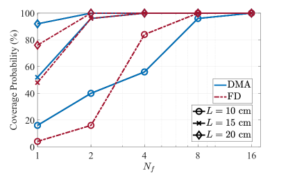
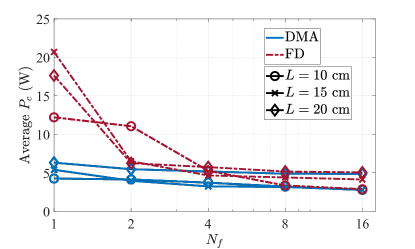
Figure 8: (a) Coverage probability (left) and (b) average power consumption (right) as a function of $N_{f}$ for the single-user scenario..

As earlier mentioned, the HPA is the most power-consuming component in the WPT system and its specific power consumption depends on the HPA output power. Interestingly, the DMA power consumption does not depend much on $N_{f}$. Specifically, since $N_{rf}$ is much smaller for DMA compared to FD, more transmit power should be provided at the HPAs output to meet the EH requirements unless $L$ and $N_{rf}$ are significantly large. Hence, based on the discussions in Section III-D, the HPAs work closer to the saturation level with higher efficiencies in a DMA structure and this leads to negligible changes in power consumption over different $N_{f}$ values. On the other hand, FD uses more RF chains, thus, the average HPA output power is lower and the power consumption becomes considerably lower when considering a large enough $N_{f}$. The reason is the high-efficiency Doherty HPA which makes it possible for the RF chains in the FD case to utilize the HPA that is working with a lower saturation level, thus, consuming less power when the output power is relatively small. Meanwhile, the FD average power consumption increases when $N_{f}$ is relatively small because of the low coverage probability in this case. Note that the power consumption increases with the antenna array size for sufficiently large $N_{f}$ because more RF chains are implemented. On the other hand, this may not hold for small $N_{f}$ and depends on the beamforming capability provided by the number of elements, signals, and transmit tones. For example, a 400 cm² FD array consumes less power than a 100 cm² for $N_{f}=2$. The reason is that the coverage probability is considerably smaller for the latter case, and the available beamforming degrees of freedom are insufficient. Additionally, the same reasoning applies to the DMA, with the exception that while the coverage probability gap between different $L$ values may be substantial, the average power consumption gap is not. This is due to the HPAs operating near the saturation region with maximum power consumption.

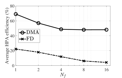
Figure 9: Average HPA efficiency for $M=1$ and $L=20$ cm as a function of $N_{f}$.

Fig. 9 represents the HPA efficiency results for further insights and clarification. Herein, we set $L=20$ cm and $M=1$ for a fair comparison between FD and DMA as both achieve 100$\%$ coverage probability for $N_{f}\geq 2$ in this case. It is observed that the HPAs of the DMA are operating with much higher efficiency compared to FD. Furthermore, less HPA output power is needed to meet the EH requirements when considering more transmit tones, and thus, the efficiency decreases with $N_{f}$. There is also another reason for higher output power ranges in the DMA that is worth discussing. As mentioned earlier, the RF chain output signal is affected by the microstrip propagation and metamaterial element losses in this architecture. Therefore, it is desirable to have more HPA output power to compensate for these losses. Meanwhile, it is assumed that the signal in FD does not experience such a condition and it is directly transmitted without any further loss at the radiating elements. It should be noted that HPA efficiency plays a crucial role in minimizing heat generation within the system due to power losses. Furthermore, this heat must be dissipated using cooling mechanisms, which consume additional power.

It is important to discuss the influence of the Doherty HPA on the system performance. Imagine that the HPA operating at a lower saturation level in the Doherty structure is referred to as HPA1, while the other one is denoted as HPA2. It was observed that the DMA and FD are only utilizing the HPA1 and HPA2, respectively. It means that if the transmitter only utilizes a single class-B HPA with a saturation level of $P_{max}$, the DMA performance is not much affected but the FD performance may be considerably degraded. For instance, in the Doherty structure, the maximum power consumption of the HPA1 and HPA2 are approximately $\frac{1}{\pi}P_{max}$ and $\frac{4}{\pi}P_{max}$, respectively. This implies that using a single HPA2, the power consumption of each HPA may be quadrupled in the FD scenario. Therefore, the implementation of the Doherty structure can offer advantages for the FD case because of the low output powers. Conversely, in the DMA architecture, Doherty HPA is only beneficial when the array size, and consequently, the number of RF chains, are large enough to ensure that each HPA operates at a lower output power level.

Although increasing the number of transmit tones can lead to high PAPR and greater RF-to-DC conversion efficiency at the rectifier, it may degrade the performance in case of the HPAs operating in the saturation and high distortion region [14]. On the other hand, we showed that the output power of the HPA determines the HPA power consumption and since the goal of the optimization algorithm is to minimize the power consumption, we expect it to force the HPAs to operate below the saturation region where the signal distortion level is negligible and the system consumes less power. Fig. 10 illustrates the received signal, the amplitude of the designed waveform, and the weights at the input of the first HPA for the single-user setup. Interestingly, Fig. 10.b proves that the input power to the HPA is below the saturation level, and thus, the EH non-linearity is the dominant factor in the simulated scenario. Furthermore, the results indicate that the received signal experiences high peak amplitudes at specific intervals to leverage the rectifier non-linearity. Additionally, it is seen that most of the tones are utilized and allocated power, leading to enhanced performance when multiple transmit tones are employed.

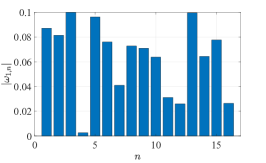
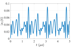
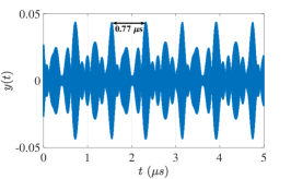
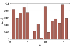
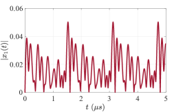
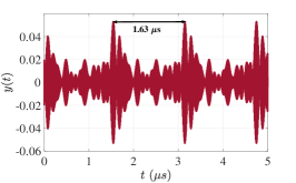
Figure 10: Waveform for $N_{f}=16$ and a single user at the area center for a 100 cm² DMA (top) and fully-digital architecture (bottom). (a) The first HPA digital precoding weights amplitude (left), (b) amplitude of the first HPA input signal (middle), and (c) received RF signal (right).

V-B Multi-User Setup

Herein, the charging of multiple devices is considered. Fig. 11 illustrates the coverage probability and power consumption results for $M=2$ and $M=4$. It is evident that the performance gap between DMA and FD does not follow a clear trend and it depends on the number of users, the number of tones, and the antenna size. More specifically, the performance gap may increase with the antenna array size in the small $N_{f}$ region in favor of DMA depending on the number of users. This gap is dependant on the available beamforming capability according to the number of signals (RF chains), tones, and elements to meet the EH requirements for a particular number of users. To be more precise, it is hard to meet the EH requirements for small $N_{f}$, $N_{rf}$, and arrays, thus, DMA performs better than FD in this case due to the larger number of radiating elements. Notably, FD may outperform DMA when $N_{f}$ is relatively large due to the increased flexibility in terms of available transmit power (i.e., greater transmit power range) and the possibility of leveraging the rectifier non-linearity more efficiently.

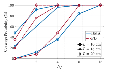
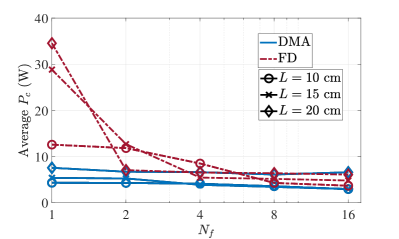
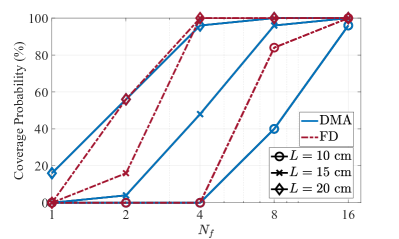
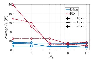
Figure 11: Coverage probability (left) and average power consumption (right), for (a) $M=2$ (top) and (b) $M=4$ (bottom), as a function of $N_{f}$.

Similar to the single-user scenario, the DMA power consumption slightly changes with $N_{f}$, while the FD’s considerably decreases with $N_{f}$. In general, the power consumption of DMA remains below FD when $N_{f}$ is relatively small. For example, the power consumption of a 400 cm² DMA array for charging 4 EH devices is under 10 W for different $N_{f}$ values. Meanwhile, an FD with the same size consumes much more power when $N_{f}<4$, and almost similar to DMA for $N_{f}>4$. Moreover, 100 $\%$ coverage probability is achieved for $M=4$ with $N_{f}=8$ and a 400 cm² DMA or FD. Although the power consumption is almost similar for these two cases of full coverage, the number of RF chains, and thus, complexity and cost are considerably smaller in DMA. Additionally, as we previously discussed, the implementation of the Doherty HPA leads to a reduction in power consumption for the FD setup, bringing it closer to the power consumption level of the DMA case. Furthermore, the power consumption increases with the number of users because more transmit power is required for meeting the EH requirements. On the other hand, it is obvious that larger $M$ may lead to lower coverage probability.

The influence of the shape of the antenna array is another factor worth investigating. For this, we consider a 100 cm² form factor constraint for antenna deployment using different rectangular shapes. Fig. 12 represents the simulation results for $M=2$ and $N_{f}=4$. It is shown that the FD performance is not affected much by the array shape since the number of RF chains is almost the same. Indeed, there are 9 RF chains in a 10 $\times$ 10 cm² FD antenna array and 8 RF chains for the rest of the FD shapes. On the other hand, increasing the number of RF chains may be favorable for DMA because more amplified signals will be available for power transmission. However, having more RF chains leads to greater power consumption and a smaller number of metamaterial elements given form factor constraints. Therefore, there is an optimum array shape and a corresponding number of RF chains to be deployed. Notice that a 12.5 $\times$ 8 cm² DMA provides the greatest coverage probability with less power consumption than its competitor the 25 $\times$ 4 cm² array. Also, the 12.5 $\times$ 8 cm² DMA provides the same coverage probability as the best FD case with considerably lower power consumption. In general, there is an optimal DMA shape for each setup depending on the system parameters which may outperform the FD structure with the same size. Note that the DMA passive losses, which are caused by the propagation inside the microstrips, can also degrade the performance in case of using a significantly large number of metamaterial elements. On the other hand, utilizing only a few metamaterial elements does not provide sufficient beamforming capability to meet the EH requirements.

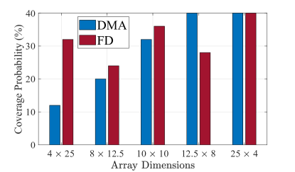
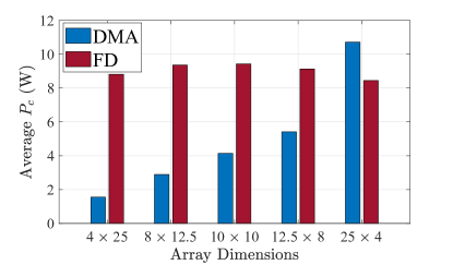
Figure 12: Simulation results for different rectangular array shapes, with $N_{f}=4$ and $M=2$. (a) Coverage probability (left) and (b) average power consumption (right).

Some discussions on the complexity of implementing a large-scale FD setup are in order. Notice that 36 RF chains are needed in a 400 cm² FD array and just 6 for a DMA with the same size. Thus, it is reasonable to implement DMA because of the lower complexity, cost, and better performance when $N_{f}$ and $L$ are small. Additionally, the smaller number of RF chains in the DMA-assisted system leads to the HPAs operating with higher efficiency, unless $L$ is significantly large. All in all, choosing suitable parameters is imperative to provide suitable beamforming capabilities. More precisely, each RF chain provides a signal for power transmission purpose, which together with a greater $N_{f}$, allows a more granular beamforming tuning. Thus, one should consider the number of EH devices, area size, antenna array size, and number of tones to achieve the best performance.

VI Conclusion and Future Work

In this paper, we investigated a MISO WPT system with fully-digital and DMA-based transmit architectures to charge multiple devices while considering the main non-linearities in the system. Furthermore, we utilized the high-efficiency Doherty HPA and provided a solution based on PSO for the joint waveform and beamforming optimization problem to minimize the system power consumption, while delivering a predefined amount of DC power to all the users. Numerical results showed that the coverage probability and power consumption improve by increasing the number of waveform tones. Furthermore, we found that DMA performs better than FD when the antenna size and number of tones are small. Although FD may outperform DMA when utilizing a relatively large number of transmit tones, it is more complex and costly because of the larger number of RF chains. Meanwhile, it was observed that a properly shaped DMA array may perform better than a fully-digital array of the same size, even in scenarios involving a large number of transmit tones. Conversely, the shape does not have much impact on a fully-digital setup. Moreover, results proved that the average HPA efficiency in a DMA-based architecture is much higher compared to a fully-digital structure. Additionally, the Doherty HPA is beneficial for reducing the power consumption in the fully-digital architecture due to the HPAs operating in lower output power ranges compared to the DMA-assisted structure. In general, one should choose the antenna size, number of tones, and antenna shape based on the number of users to be charged simultaneously and the deployment area to achieve the best performance in terms of coverage probability and power consumption.

As a prospect for future research, we may delve deeper into the signal generation aspect by analyzing the power consumption based on the number of transmit tones. Moreover, another interesting research direction is to utilize optimization approaches with lower complexity, e.g., relying on machine learning, to learn online the input-output relation of the system’s non-linear components while optimizing the transmit waveform accordingly.

Appendix A Microstrip Propagation Model for the DMA

We use the formulation provided in [41] to calculate the attenuation and propagation coefficients of the microstrip. We consider a microstrip line consisting of a conductor of width $W_{ms}$ printed on a dielectric substrate of thickness $d_{ms}$ with dielectric constant $\epsilon_{r}$ and $\nu=\frac{d_{ms}}{W_{ms}}$. Hereby, the effective dielectric constant can be calculated as

$$\epsilon_{e}=\frac{\epsilon_{r}+1}{2}+\frac{\epsilon_{r}-1}{2}\frac{1}{\sqrt{1+12\nu}}.$$ (29)

Furthermore, the propagation constant inside the microstrip is $\beta=k_{0}\sqrt{\epsilon_{e}}$, where $k_{0}=\frac{2\pi}{\lambda}$ is the free space propagation constant. The attenuation due to the dielectric loss is given by

$$\alpha_{d}=\frac{k_{0}\epsilon_{r}(\epsilon_{e}-1)\tan\delta}{2\sqrt{\epsilon_{e}}(\epsilon_{r}-1)}\quad\text{({Np}/m)},$$ (30)

where $\tan\delta$ is the loss tangent of the dielectric and the approximate attenuation caused by the conductor loss is given by

$$\alpha_{c}=\frac{R_{s}}{Z_{0}W_{ms}}\quad\text{({Np}/m)},$$ (31)

where $R_{s}=\sqrt{\omega\mu_{0}/2\sigma}$ is the surface resistivity of the conductor with $\sigma$ and $\mu_{0}$ being the conductivity of the conductor and the permeability of the free space, respectively. Thus, the total attenuation coefficient of the microstrip line is $\alpha=\alpha_{d}+\alpha_{c}$. Additionally, we assume that all microstrips are of the same type, in which case we can consider $\beta_{i}=\beta$ and $\alpha_{i}=\alpha$.

References

- [1] Z. Zhang et al., “6G wireless networks: vision, requirements, architecture, and key technologies,” IEEE Veh. Technol. Mag., vol. 14, no. 3, pp. 28–41, 2019.
- [2] N. H. Mahmood et al., “Six key features of machine type communication in 6G,” in 2nd 6G SUMMIT, pp. 1–5, 2020.
- [3] O. L. A. López et al., “Massive wireless energy transfer: enabling sustainable IoT toward 6G era,” IEEE Internet Things J., vol. 8, no. 11, pp. 8816–8835, 2021.
- [4] Y. Zeng et al., “Communications and signals design for wireless power transmission,” IEEE Trans Commun, vol. 65, no. 5, pp. 2264–2290, 2017.
- [5] B. Clerckx et al., “Wireless power transfer for future networks: Signal processing, machine learning, computing, and sensing,” IEEE J. Sel. Top. Signal Process., vol. 15, no. 5, pp. 1060–1094, 2021.
- [6] A. Boaventura et al., “Optimum behavior: Wireless power transmission system design through behavioral models and efficient synthesis techniques,” IEEE Microw. Mag., vol. 14, no. 2, pp. 26–35, 2013.
- [7] C. R. Valenta, M. M. Morys, and G. D. Durgin, “Theoretical energy-conversion efficiency for energy-harvesting circuits under power-optimized waveform excitation,” IEEE Trans. Microw. Theory Tech., vol. 63, no. 5, pp. 1758–1767, 2015.
- [8] A. S. Boaventura et al., “Maximizing dc power in energy harvesting circuits using multisine excitation,” in 2011 IEEE MTT-S Int. Microw. Symp., pp. 1–4, 2011.
- [9] O. L. A. López et al., “Massive MIMO with radio stripes for indoor wireless energy transfer,” IEEE Trans. Wirel. Commun., vol. 21, no. 9, pp. 7088–7104, 2022.
- [10] S. Shen and B. Clerckx, “Beamforming Optimization for MIMO Wireless Power Transfer With Nonlinear Energy Harvesting: RF Combining Versus DC Combining,” IEEE Trans. Wirel. Commun., vol. 20, no. 1, pp. 199–213, 2021.
- [11] O. L. A. López et al., “A Low-Complexity Beamforming Design for Multiuser Wireless Energy Transfer,” IEEE Wireless Commun. Lett., vol. 10, no. 1, pp. 58–62, 2021.
- [12] B. Clerckx and E. Bayguzina, “Low-Complexity Adaptive Multisine Waveform Design for Wireless Power Transfer,” IEEE Antennas Wirel. Propag. Lett., vol. 16, pp. 2207–2210, 2017.
- [13] Y. Huang and B. Clerckx, “Large-Scale Multiantenna Multisine Wireless Power Transfer,” IEEE Trans. Signal Process., vol. 65, no. 21, pp. 5812–5827, 2017.
- [14] Y. Zhang and B. Clerckx, “Waveform Design for Wireless Power Transfer With Power Amplifier and Energy Harvester Non-Linearities,” IEEE Trans. Signal Process., pp. 1–15, 2023.
- [15] S. Shen and B. Clerckx, “Joint Waveform and Beamforming Optimization for MIMO Wireless Power Transfer,” IEEE Trans Commun, vol. 69, no. 8, pp. 5441–5455, 2021.
- [16] Z. Feng et al., “Waveform and Beamforming Design for Intelligent Reflecting Surface Aided Wireless Power Transfer: Single-User and Multi-User Solutions,” IEEE Trans. Wirel. Commun., vol. 21, no. 7, pp. 5346–5361, 2022.
- [17] J. Joung et al., “A Survey on Power-Amplifier-Centric Techniques for Spectrum- and Energy-Efficient Wireless Communications,” IEEE Commun. Surv. Tutor., vol. 17, no. 1, pp. 315–333, 2015.
- [18] H. Ochiai, “An Analysis of Band-limited Communication Systems from Amplifier Efficiency and Distortion Perspective,” IEEE Trans Commun, vol. 61, no. 4, pp. 1460–1472, 2013.
- [19] I. Ahmed et al., “A Survey on Hybrid Beamforming Techniques in 5G: Architecture and System Model Perspectives,” IEEE Commun. Surv. Tutor., vol. 20, no. 4, pp. 3060–3097, 2018.
- [20] X. Gao et al., “Energy-Efficient Hybrid Analog and Digital Precoding for MmWave MIMO Systems With Large Antenna Arrays,” IEEE J. Sel. Areas Commun., vol. 34, no. 4, pp. 998–1009, 2016.
- [21] Q. Wu et al., “Intelligent Reflecting Surface-Aided Wireless Communications: A Tutorial,” IEEE Trans Commun, vol. 69, no. 5, pp. 3313–3351, 2021.
- [22] N. Shlezinger et al., “Dynamic Metasurface Antennas for 6G Extreme Massive MIMO Communications,” IEEE Wirel. Commun., vol. 28, no. 2, pp. 106–113, 2021.
- [23] B. Zheng et al., “A Survey on Channel Estimation and Practical Passive Beamforming Design for Intelligent Reflecting Surface Aided Wireless Communications,” IEEE Commun. Surv. Tutor., vol. 24, no. 2, pp. 1035–1071, 2022.
- [24] H. Zhang et al., “Near-field wireless power transfer with dynamic metasurface antennas,” in IEEE SPAWC, pp. 1–5, 2022.
- [25] A. Azarbahram et al., “Energy Beamforming for RF Wireless Power Transfer with Dynamic Metasurface Antennas,” Submitted to IEEE Wireless Commun. Lett., 2023.
- [26] Y. Zhao et al., “IRS-Aided SWIPT: Joint Waveform, Active and Passive Beamforming Design Under Nonlinear Harvester Model,” IEEE Trans Commun, vol. 70, no. 2, pp. 1345–1359, 2022.
- [27] D. R. Smith et al., “Analysis of a Waveguide-Fed Metasurface Antenna,” Phys. Rev. Appl., vol. 8, p. 054048, Nov 2017.
- [28] H. Zhang et al., “Beam focusing for near-field multiuser MIMO communications,” IEEE Trans. Wirel. Commun., vol. 21, no. 9, pp. 7476–7490, 2022.
- [29] S. W. Ellingson, “Path Loss in Reconfigurable Intelligent Surface-Enabled Channels,” in IEEE PIMRC, pp. 829–835, 2021.
- [30] C. Rapp, “Effects of HPA-nonlinearity on a 4-DPSK/OFDM-signal for a digital sound broadcasting signal,” ESA Special Publication, vol. 332, pp. 179–184, 1991.
- [31] L. You et al., “Energy Efficiency Maximization of Massive MIMO Communications With Dynamic Metasurface Antennas,” IEEE Trans. Wirel. Commun., vol. 22, no. 1, pp. 393–407, 2023.
- [32] B. Clerckx and E. Bayguzina, “Waveform Design for Wireless Power Transfer,” IEEE Trans. Signal Process., vol. 64, no. 23, pp. 6313–6328, 2016.
- [33] B. Kim et al., “The Doherty power amplifier,” IEEE Microw. Mag., vol. 7, no. 5, pp. 42–50, 2006.
- [34] C. Lin and G. Y. Li, “Energy-Efficient Design of Indoor mmWave and Sub-THz Systems With Antenna Arrays,” IEEE Trans. Wirel. Commun., vol. 15, no. 7, pp. 4660–4672, 2016.
- [35] J. Kennedy and R. Eberhart, “Particle swarm optimization,” in Proc. Int. Conf. on Neural Networks, vol. 4, pp. 1942–1948 vol.4, 1995.
- [36] I. C. Trelea, “The particle swarm optimization algorithm: convergence analysis and parameter selection,” Inf. Process. Lett., vol. 85, no. 6, pp. 317–325, 2003.
- [37] R. C. Eberhart, Y. Shi, and J. Kennedy, Swarm intelligence. Elsevier, 2001.
- [38] E. Mezura-Montes and C. A. Coello Coello, “Constraint-handling in nature-inspired numerical optimization: Past, present and future,” Swarm and Evolutionary Computation, vol. 1, no. 4, pp. 173–194, 2011.
- [39] M. E. H. Pedersen, “Good parameters for particle swarm optimization,” Hvass Lab., Copenhagen, Denmark, Tech. Rep. HL1001, pp. 1551–3203, 2010.
- [40] B. Clerckx and J. Kim, “On the beneficial roles of fading and transmit diversity in wireless power transfer with nonlinear energy harvesting,” IEEE Trans. Wirel. Commun., vol. 17, no. 11, pp. 7731–7743, 2018.
- [41] D. M. Pozar, Microwave engineering. John wiley & sons, 2011.