hep-th/yymmnnn

Extremal black string with Kalb-Ramond field via $\alpha^{\prime}$ corrections

Shuxuan Ying

Department of Physics, Chongqing University

Chongqing, 401331, China

ysxuan@cqu.edu.cn

Abstract

In this paper, we obtain the three-dimensional regular extremal black string solution incorporating $\alpha^{\prime}$ corrections and a non-trivial Kalb-Ramond field. The difficulty in considering the Kalb-Ramond field lies in the fact that it transforms the original equations of motion into an infinite summation form involving matrices, making it difficult to calculate the matrix differential equations. To solve this problem, we introduce a new method that transforms the infinite summation of matrix differential equations into a simple trace of the matrix. As a result, we are able to obtain a non-perturbative and non-singular extremal black string solution. Indeed, this work serves as a good example for studying more complicated non-perturbative solutions that incorporate the Kalb-Ramond field via complete $\alpha^{\prime}$ corrections.

1 Introduction

In recent studies [1, 2, 3], Hohm and Zwiebach made notable contributions to understanding the $\alpha^{\prime}$ corrections of closed string theory at all orders and derived the complete action by utilizing the $O\left(d,d\right)$ symmetry. The key point that complete action can be obtained by $O\left(d,d\right)$ symmetry is due to the fact that when massless closed string fields are independent of the $m$ coordinates, the action manifests an $O\left(m,m\right)$ symmetry [4, 5]. This result has been verified in the tree-level string effective action as well as its first-order $\alpha^{\prime}$ correction. Consequently, it suggests that the low energy effective action with complete $\alpha^{\prime}$ corrections can be expressed by utilizing the standard $O\left(d,d\right)$ matrix in terms of $\alpha^{\prime}$ corrected fields for time-dependent backgrounds [6, 4, 5, 7, 8]. Based on this observation, Hohm and Zwiebach conjectured that this result is always true for all orders in $\alpha^{\prime}$. Conjectured this assumption, they successfully demonstrated that the $\alpha^{\prime}$ corrections can be classified based on even powers of the Hubble parameter within the framework of the FLRW cosmological background. In addition, it is worth noting that the dilaton field only includes first-order time derivatives. These features make the equations of motion (EOM) to solely include two derivatives of the metric and be exactly solvable. This remarkable progress introduces a new action that make the study of black holes and cosmology incorporating non-perturbative string effects possible. By using this action, numerous new regular black hole solutions and cosmological solutions were studied. Refs. [9, 10, 11, 12, 13, 14] have considered the FLRW cosmological ansatz, revealing that the $\alpha^{\prime}$ corrections can eliminate the big bang singularity. In addition, the resolution of curvature singularities in two-dimensional string black holes has been discussed in refs. [15, 16, 17, 18]. However, these solutions impose significant constraints on the form of the spacetime ansatz and require the Kalb-Ramond field to vanish. It looks impossible to get the non-perturbative solutions with a non-constant Kalb-Ramond field. The challenge arises from the fact that considering the Kalb-Ramond field makes the classification of $\alpha^{\prime}$ corrections complicated, which can no longer be simply written by even powers of the Hubble parameter. Instead, an infinite summation of $O\left(d,d\right)$ matrices must be considered. The previous discussion about Kalb-Ramond field in Hohm-Zwiebach action can be found in a ref. [19]. To demonstrate the difficulty including Kalb-Ramond field, let us recall the Hohm-Zwiebach action for the black hole background:

$$I_{HZ}=-\int dx^{3}e^{-\Phi}\left(-\dot{\Phi}^{2}+\stackrel{{\scriptstyle[}}{{k}}=1]{\infty}{\sum}\left(\alpha^{\prime}\right)^{k-1}\bar{c}_{k}\mathrm{Tr}\left(\dot{\mathcal{S}}^{2k}\right)\right),$$ (1.1)

where all fields depend on $y$, and $\dot{f}\left(y\right)\equiv\partial_{y}f\left(y\right)$. The coefficients are $\bar{c}_{1}=c_{1}=-\frac{1}{8}$, $\bar{c}_{2}=-c_{2}=-\frac{1}{64}$, $\bar{c}_{3}=c_{3}=-\frac{1}{3.2^{7}}$, $\bar{c}_{4}=-c_{4}=-\frac{1}{2^{15}}+\frac{1}{2^{12}}\zeta\left(3\right)$ and $\bar{c}_{k>4}$’s are unknown coefficients for the bosonic case [20]. The $O\left(d,d\right)$ invariant dilaton and $O\left(d,d\right)$ matrix are defined as

$$e^{-\Phi}\equiv\sqrt{g}e^{-2\phi},\qquad\mathcal{S}=\left(\begin{array}[]{cc}BG^{-1}&G-BG^{-1}B\\ G^{-1}&-G^{-1}B\end{array}\right),$$ (1.2)

where $\phi$ is the physical dilaton, and $g$ does not include the direction of $dy$. The EOM derived from the action are given by:

$$\ddot{\Phi}-\stackrel{{\scriptstyle[}}{{k}}=1]{\infty}{\sum}\left(\alpha^{\prime}\right)^{k-1}k\bar{c}_{k}\mathrm{Tr}\left(\dot{\mathcal{S}}\right)^{2k} = 0,$$ (1.3)

$$\frac{d}{dy}\left(e^{-\Phi}\stackrel{{\scriptstyle[}}{{k}}=1]{\infty}{\sum}\left(\alpha^{\prime}\right)^{k-1}4k\bar{c}_{k}\mathcal{S}\left(\dot{\mathcal{S}}\right)^{2k-1}\right) = 0,$$ (1.4)

$$\dot{\Phi}^{2}-\stackrel{{\scriptstyle[}}{{k}}=1]{\infty}{\sum}\left(\alpha^{\prime}\right)^{k-1}\left(2k-1\right)\bar{c}_{k}\mathrm{Tr}\left(\dot{\mathcal{S}}\right)^{2k} = 0.$$ (1.5)

If we consider the three-dimensional black hole ansatz without the Kalb-Ramond field:

$$ds^{2}=a\left(y\right)^{2}\left(-dt^{2}+dx^{2}\right)+dy^{2}.$$ (1.6)

The EOM (1.3) to (1.5) can be significantly simplified as follows:

$$\dot{\Phi}+\frac{1}{2}\bar{H}\bar{f}\left(\bar{H}\right) = 0,$$

$$\frac{d}{dy}\left(e^{-\Phi}\bar{f}\left(\bar{H}\right)\right) = 0,$$

$$\dot{\Phi}+\bar{g}\left(\bar{H}\right) = 0,$$ (1.7)

where the Hubble parameter is defined as $\bar{H}\left(y\right)=\frac{\dot{a}\left(y\right)}{a\left(y\right)}$ and

$$\bar{f}\left(\bar{H}\right) = d\stackrel{{\scriptstyle[}}{{k}}=1]{\infty}{\sum}\left(-\alpha^{\prime}\right)^{k-1}2^{2\left(k+1\right)}k\bar{c}_{k}\bar{H}^{2k-1},$$

$$\bar{g}\left(\bar{H}\right) = d\stackrel{{\scriptstyle[}}{{k}}=1]{\infty}{\sum}\left(-\alpha^{\prime}\right)^{k-1}2^{2k+1}\left(2k-1\right)\bar{c}_{k}\bar{H}^{2k}.$$ (1.8)

In these EOM (1.7), if we start with the non-perturbative and non-singular dilaton solution $\Phi$ obtained from the perturbative solution, we can obtain $\bar{f}\left(\bar{H}\right)$ and $\bar{g}\left(\bar{H}\right)$ directly. Since the non-perturbative expansions (1.8) introduces an extra constraint $\dot{\bar{g}}=\bar{H}\dot{\bar{f}}$, we can also determine $\bar{H}$ in the subsequent step. In other words, all solutions can be derived from $\Phi$. However, when considering a non-trivial Kalb-Ramond field, we can only utilize the complicated EOM (1.3) to (1.5). The solution $\Phi$ in these EOM cannot determine the solution of the matrix $\mathcal{S}$ due to equation (1.4), which includes an infinite summation of matrices, and we cannot extract any constraints such as $\dot{\bar{g}}=\bar{H}\dot{\bar{f}}$ from equations (1.3) to (1.5). The solution $\Phi$ in these EOM cannot determine the solution of the matrix $\mathcal{S}$ due to the equation (1.4) includes infinite summation of matrices, and we can not extract any constraint such as $\dot{\bar{g}}=\bar{H}\dot{\bar{f}}$ from the (1.3) to (1.5). Therefore, it seems impossible to obtain the non-perturbative solution including the Kalb-Ramond field.

In this paper, our aim is to develop a method for calculating the non-perturbative and non-singular solutions of the Hohm-Zwiebach action, including a non-trivial Kalb-Ramond field. We begin with the three-dimensional black string solution with axion charge [21, 22]. When $\left|Q\right|=M$ and we set $\lambda\rightarrow\infty$ of cosmological constant $8/\lambda$, the metric becomes extremal, which corresponds to the fields outside the fields outside a fundamental macroscopic string [23]:

$$ds^{2}=\frac{1}{y}\left(-dt^{2}+dx^{2}\right)+dy^{2},$$ (1.9)

This extremal metric includes a non-trivial Kalb-Ramond field and exhibits a naked singularity. Our method aims to remove this singularity, and it can be summarized as follows: At first, we extract the ansatz based on the extremal metric (1.9) and derive the corresponding Hohm-Zwiebach action. Secondly, we calculate the perturbative solution up to the first order of $\alpha^{\prime}$ correction of the action. The key point in this step is that, when we integrate out $d/dy$ from the matrix different equation (1.4), the constant matrix solution may also receive $\alpha^{\prime}$ corrections. Furthermore, we observe that in our perturbative solution, the dilaton does not receive $\alpha^{\prime}$ corrections; only the metric and the Kalb-Ramond field are affected. Thirdly, we use a trick to transform the infinite summation of the matrix differential equation (1.4) into a simple trace equation:

$$4e^{-\Phi}\left[\stackrel{{\scriptstyle[}}{{k}}=1]{\infty}{\sum}\left(\alpha^{\prime}\right)^{k-1}kc_{k}\mathrm{Tr}\left(\dot{\mathcal{S}}\right)^{2k}\right]=\mathrm{Tr}\left(\mathbb{C}\mathcal{S}^{-1}\dot{\mathcal{S}}\right),$$ (1.10)

where $\mathbb{C}$ is $4\times 4$ constant matrix. Reconsidering the EOM (1.3), (1.4) and (1.10), we find that all fields depend on $\Phi$, allowing us to determine the solution of $\mathcal{S}$ through equation (1.10). Finally, we obtain the regular solution of these EOM, and it implies that the naked curvature singularity of three-dimensional extremal black string solution can be successfully removed. As expected, the regular solution matches the perturbative solution in the perturbative limit $\alpha^{\prime}\rightarrow 0$. While our regular solution currently matches only the first two orders of the perturbative solution, it can be easily generalized to arbitrary orders using our previous method [10].

The remainder of this paper is outlined as follows: In section 2, we briefly review the three-dimensional extremal black string at the tree-level. In section 3, we calculate the non-perturbative and non-singular extremal black hole solution, including Kalb-Ramond field. Section 4 is a conclusion.

2 Three-dimensional extremal black string at tree-level

In this section, we demonstrate how to obtain the three-dimensional extremal black string solution from the tree-level low energy effective action of bosonic closed string theory. We start with the three-dimensional low energy effective action given by:

$$I_{0}=\int d^{3}x\sqrt{-g}e^{-2\phi}\left(R+4\left(\partial\phi\right)^{2}-\frac{1}{12}H^{2}\right),$$ (2.11)

where $R$ is the Ricci scalar for the metric $g_{\mu\nu}$, $\phi$ represents the dilaton, and $H_{\mu\nu\rho}=3\partial_{\left[\mu\right.}b_{\left.\nu\rho\right]}$ is the field strength of the anti-symmetric Kalb-Ramond field $b$. Next, we consider the following ansatz:

$$ds^{2}=a\left(y\right)^{2}\left(-dt^{2}+dx^{2}\right)+dy^{2}.$$ (2.12)

This ansatz can also be written as:

$$g_{\mu\nu}=\left(\begin{array}[]{ccc}-a^{2}\left(y\right)&0&0\\ 0&a^{2}\left(y\right)&0\\ 0&0&1\end{array}\right),\qquad b_{\mu\nu}=\left(\begin{array}[]{ccc}0&b_{tx}\left(y\right)&0\\ b_{xt}\left(y\right)&0&0\\ 0&0&0\end{array}\right),\qquad\phi=\phi\left(y\right).$$ (2.13)

It is important to note that $b_{tx}\left(y\right)=-b_{xt}\left(y\right)$. Since the ansatz (2.12) is independent of $y$, we can introduce the following notation to manifest the $O\left(2,2\right)$ symmetry:

$$g_{\mu\nu}=\left(\begin{array}[]{cc}G_{ij}\left(y\right)&0\\ 0&1\end{array}\right),\qquad b_{\mu\nu}=\left(\begin{array}[]{cc}B_{ij}\left(y\right)&0\\ 0&0\end{array}\right),$$ (2.14)

where

$$G_{ij}\left(y\right)\equiv\left(\begin{array}[]{cc}-a^{2}\left(y\right)&0\\ 0&a^{2}\left(y\right)\end{array}\right),\qquad B_{ij}\left(y\right)\equiv\left(\begin{array}[]{cc}0&b_{tx}\left(y\right)\\ b_{xt}\left(y\right)&0\end{array}\right).$$ (2.15)

With this notation, the action (2.11) can be rewritten as:

$$I_{0}=-\int dx^{3}e^{-\Phi}\left(-\dot{\Phi}^{2}-\frac{1}{8}\mathrm{Tr}\left(\dot{\mathcal{S}}^{2}\right)\right),$$ (2.16)

where the dot denotes a derivative with respect to $y$, i.e., $\dot{f}\left(y\right)\equiv\partial_{y}f\left(y\right)$, and

$$\mathcal{S}=\left(\begin{array}[]{cc}BG^{-1}&G-BG^{-1}B\\ G^{-1}&-G^{-1}B\end{array}\right).$$ (2.17)

The $O\left(d,d\right)$ invariant dilaton $\Phi$ in action (2.16) is defined in the action as:

$$\Phi=2\phi-\frac{1}{2}\ln\left|\det G_{ij}\right|.$$ (2.18)

The EOM for the action (2.16) are as follows:

$$\ddot{\Phi}+\frac{1}{8}\mathrm{Tr}\left(\dot{\mathcal{S}}\right)^{2} = 0,$$

$$\frac{d}{dy}\left(e^{-\Phi}\mathcal{S}\left(\dot{\mathcal{S}}\right)\right) = 0,$$

$$\dot{\Phi}^{2}+\frac{1}{8}\mathrm{Tr}\left(\dot{\mathcal{S}}\right)^{2} = 0.$$ (2.19)

The simplest solution that includes a non-trivial Kalb-Ramond field is:

$$\Phi=0,\qquad a\left(y\right)=\frac{1}{\sqrt{y}},\qquad b_{tx}\left(y\right)=\frac{1}{y}.$$ (2.20)

The corresponding Kretschmann scalar is given by:

$$R_{\mu\nu\rho\sigma}R^{\mu\nu\rho\sigma}=\frac{4\left(2a^{2}\ddot{a}^{2}+\dot{a}^{4}\right)}{a^{4}}=\frac{19}{4y^{4}}.$$ (2.21)

It implies that the solution possesses a curvature singularity at $y=0$ and no event horizon. This solution describes the fields outside a fundamental macroscopic string, which corresponds to a three-dimensional extremal black string. To understand the relationship between this tree-level singular solution (2.20) and the extremal black string, let us recall the three-dimensional black string with an axion charge:

$$ds^{2}=-\left(1-\frac{M}{r}\right)dt^{2}+\left(1-\frac{Q^{2}}{Mr}\right)dx^{2}+\left(1-\frac{M}{r}\right)^{-1}\left(1-\frac{Q^{2}}{Mr}\right)^{-1}\frac{\lambda dr^{2}}{8r^{2}},$$ (2.22)

with

$$H_{rtx}=\frac{Q}{r^{2}},\qquad\phi=\ln r+\frac{1}{2}\ln\frac{\lambda}{2},$$ (2.23)

where $8/\lambda$ is related to the cosmological constant. The extremal metric is obtained by setting $\left|Q\right|=M$, which gives:

$$ds^{2}=\left(1-\frac{M}{r}\right)\left(-dt^{2}+dx^{2}\right)+\left(1-\frac{M}{r}\right)^{-2}\frac{\lambda dr^{2}}{8r^{2}}.$$ (2.24)

Using the coordinate transformations:

$$\tilde{y}=-\left(\frac{\lambda}{8}\right)^{1/2}\frac{r}{M},\qquad\tilde{t}=\left(\frac{\lambda}{8}\right)^{1/4}x,\qquad\tilde{x}=\left(\frac{\lambda}{8}\right)^{1/4}t,$$ (2.25)

and taking the limit $\lambda\rightarrow\infty$, which corresponds to the vanishing cosmological constant in the action (2.11), the extremal metric (2.24) becomes:

$$ds^{2}=\frac{1}{\tilde{y}}\left(-d\tilde{t}^{2}+d\tilde{x}^{2}\right)+d\tilde{y}^{2},$$ (2.26)

which matches the solution (2.20). In this ansatz, we can employ the isotropic Hohm-Zwiebach action without considering the multitrace terms.

3 Regular extremal black string via $\alpha^{\prime}$ corrections

In this section, our aim is to remove the naked singularity of the solution (2.20) by using the Hohm-Zwiebach action. Hohm and Zwiebach demonstrated that the following low energy effective action with complete $\alpha^{\prime}$ corrections can be expressed as

$$I_{HZ} = \int d^{3}x\sqrt{-g}e^{-2\phi}\left(R+4\left(\partial\phi\right)^{2}-\frac{1}{12}H^{2}+\frac{1}{4}\alpha^{\prime}\left(R^{\mu\nu\rho\sigma}R_{\mu\nu\rho\sigma}+\ldots\right)+\alpha^{\prime 2}\left(\ldots\right)+\ldots\right)$$ (3.27)

$$= -\int dx^{3}e^{-\Phi}\left(-\dot{\Phi}^{2}+\stackrel{{\scriptstyle[}}{{k}}=1]{\infty}{\sum}\left(\alpha^{\prime}\right)^{k-1}\bar{c}_{k}\mathrm{Tr}\left(\dot{\mathcal{S}}^{2k}\right)\right),$$

where $\bar{c}_{1}=c_{1}=-\frac{1}{8}$, $\bar{c}_{2}=-c_{2}=-\frac{1}{64}$, $\bar{c}_{3}=c_{3}=-\frac{1}{3.2^{7}}$, $\bar{c}_{4}=-c_{4}=-\frac{1}{2^{15}}+\frac{1}{2^{12}}\zeta\left(3\right)$ and $\bar{c}_{k>4}$’s are unknown coefficients for the bosonic case [20]. The EOM of the Hohm-Zwiebach action are given by:

$$\ddot{\Phi}-\stackrel{{\scriptstyle[}}{{k}}=1]{\infty}{\sum}\left(\alpha^{\prime}\right)^{k-1}k\bar{c}_{k}\mathrm{Tr}\left(\dot{\mathcal{S}}\right)^{2k} = 0,$$

$$\frac{d}{dy}\left(e^{-\Phi}\stackrel{{\scriptstyle[}}{{k}}=1]{\infty}{\sum}\left(\alpha^{\prime}\right)^{k-1}4k\bar{c}_{k}\mathcal{S}\left(\dot{\mathcal{S}}\right)^{2k-1}\right) = 0,$$

$$\dot{\Phi}^{2}-\stackrel{{\scriptstyle[}}{{k}}=1]{\infty}{\sum}\left(\alpha^{\prime}\right)^{k-1}\left(2k-1\right)\bar{c}_{k}\mathrm{Tr}\left(\dot{\mathcal{S}}\right)^{2k} = 0.$$ (3.28)

To calculate the perturbative solution, let us introduce a new variable $\Omega\equiv e^{-\Phi}$, where $\dot{\Omega}=-\dot{\Phi}\Omega$ and $\ddot{\Omega}=\left(-\ddot{\Phi}+\dot{\Phi}^{2}\right)\Omega$. The EOM can be rewritten as:

$$\frac{\left(\dot{\Omega}\right)^{2}}{\Omega^{2}}-\frac{\ddot{\Omega}}{\Omega}-\stackrel{{\scriptstyle[}}{{k}}=1]{\infty}{\sum}\left(\alpha^{\prime}\right)^{k-1}kc_{k}\mathrm{Tr}\left(\dot{\mathcal{S}}\right)^{2k} = 0,$$

$$\frac{d}{dy}\left(e^{-\Phi}\stackrel{{\scriptstyle[}}{{k}}=1]{\infty}{\sum}\left(\alpha^{\prime}\right)^{k-1}4kc_{k}\mathcal{S}\left(\dot{\mathcal{S}}\right)^{2k-1}\right) = 0,$$

$$\frac{\dot{\Omega}^{2}}{\Omega^{2}}-\stackrel{{\scriptstyle[}}{{k}}=1]{\infty}{\sum}\left(\alpha^{\prime}\right)^{k-1}\left(2k-1\right)c_{k}\mathrm{Tr}\left(\dot{\mathcal{S}}\right)^{2k} = 0,$$ (3.29)

Next, we make the assumption that the perturbative solutions of the EOM given by (3.30) take the following forms:

$$\Omega\left(y\right) = \Omega_{0}\left(y\right)+\alpha^{\prime}\Omega_{1}\left(y\right)+\alpha^{\prime 2}\Omega_{2}\left(y\right)+\ldots,$$

$$a\left(r\right) = a_{0}\left(r\right)+\alpha^{\prime}a_{1}\left(r\right)+\alpha^{\prime 2}a_{2}\left(r\right)+\ldots.$$

$$b\left(r\right) = b_{0}\left(r\right)+\alpha^{\prime}b_{1}\left(r\right)+\alpha^{\prime 2}b_{2}\left(r\right)+\ldots,$$ (3.30)

where we define $b_{tx}\left(y\right)\equiv b\left(y\right)$. Substituting the perturbative forms (3.30) into the EOM (3.30) and considering the zeroth order in $\alpha^{\prime}$, we obtain the following equations:

$$\ddot{\Omega}_{0}\left(y\right) = 0,$$

$$\dot{\Omega}_{0}^{2}+\frac{\Omega_{0}^{2}\left(\dot{b}_{0}^{2}-4a_{0}^{2}\dot{a}_{0}^{2}\right)}{2a_{0}^{4}} = 0,$$ (3.31)

and the second equation of the EOM (3.30) leads to the following expression:

$$\frac{d}{dy}\left(\begin{array}[]{cccc}\mathbb{M}_{11}^{0}&0&0&\mathbb{M}_{14}^{0}\\ 0&\mathbb{M}_{11}^{0}&-\mathbb{M}_{14}^{0}&0\\ 0&-\mathbb{M}_{41}^{0}&\mathbb{M}_{44}^{0}&0\\ \mathbb{M}_{41}^{0}&0&0&\mathbb{M}_{44}^{0}\end{array}\right)=0,$$ (3.32)

where the entries of the matrix are given by

$$\mathbb{M}_{11}^{0} = \frac{\Omega_{0}\left(2a_{0}^{3}\dot{a}_{0}-b_{0}\dot{b}_{0}\right)}{2a_{0}^{4}},$$

$$\mathbb{M}_{41}^{0} = \frac{\Omega_{0}\dot{b}_{0}}{2a_{0}^{4}},$$

$$\mathbb{M}_{14}^{0} = \frac{\Omega_{0}\left(4a_{0}^{3}\dot{a}_{0}b-\left(a_{0}^{4}+b_{0}^{2}\right)\dot{b}_{0}\right)}{2a_{0}^{4}},$$

$$\mathbb{M}_{44}^{0} = \frac{\Omega_{0}\left(b_{0}\dot{b}_{0}-2a_{0}^{3}\dot{a}_{0}\right)}{2a_{0}^{4}}.$$ (3.33)

The solution is

$$\Omega_{0}=1,\qquad a_{0}=\frac{1}{\sqrt{y}},\qquad b_{0}=\frac{1}{y},$$ (3.34)

which is consistent with the solution (2.20). The integration of $d/dy$ in the second equation of EOM (3.29) yields the constant matrix

$$\left(\begin{array}[]{cccc}\mathbb{M}_{11}^{0}&0&0&\mathbb{M}_{14}^{0}\\ 0&\mathbb{M}_{11}^{0}&-\mathbb{M}_{14}^{0}&0\\ 0&-\mathbb{M}_{41}^{0}&\mathbb{M}_{44}^{0}&0\\ \mathbb{M}_{41}^{0}&0&0&\mathbb{M}_{44}^{0}\end{array}\right)=\left(\begin{array}[]{cccc}0&0&0&0\\ 0&0&0&0\\ 0&-1&0&0\\ 1&0&0&0\end{array}\right).$$ (3.35)

This constant matrix plays a crucial role in determining the non-perturbative solution. Considering the EOM (3.30) at the first order of $\alpha^{\prime}$, we have:

$$\ddot{\Omega}_{1}+\frac{\Omega_{0}\left(\dot{b}_{0}^{2}-4a_{0}^{2}\dot{a}_{0}^{2}\right){}^{2}}{16a_{0}^{8}} = 0,$$

$$2\dot{\Omega}_{0}\dot{\Omega}_{1}+\frac{\Omega_{0}\Omega_{1}\left(\dot{b}_{0}^{2}-4a_{0}^{2}\dot{a}_{0}^{2}\right)}{a_{0}^{4}}$$

$$+\Omega_{0}^{2}\left(\frac{3\left(\dot{b}_{0}^{2}-4a_{0}^{2}\dot{a}_{0}^{2}\right){}^{2}}{16a_{0}^{8}}+\frac{a_{0}\dot{b}_{0}\dot{b}_{1}-2a_{1}\dot{b}_{0}^{2}-4a_{0}^{3}\dot{a}_{0}\dot{a}_{1}+4a_{1}a_{0}^{2}\dot{a}_{0}^{2}}{a_{0}^{5}}\right) = 0,$$

and

$$\frac{d}{dy}\left(\begin{array}[]{cccc}\mathbb{M}_{11}^{1}&0&0&\mathbb{M}_{14}^{1}\\ 0&\mathbb{M}_{11}^{1}&-\mathbb{M}_{14}^{1}&0\\ 0&-\mathbb{M}_{41}^{1}&\mathbb{M}_{44}^{1}&0\\ \mathbb{M}_{41}^{1}&0&0&\mathbb{M}_{44}^{1}\end{array}\right)=0,$$ (3.36)

where

$$\mathbb{M}_{11}^{1} = -\frac{1}{8a_{0}^{8}}\left[4a_{0}^{4}\left(\left(b_{1}\Omega_{0}+b_{0}\Omega_{1}\right)\dot{b}_{0}+\Omega_{0}b_{0}\dot{b}_{1}\right)-2a_{0}^{3}\Omega_{0}\dot{b}_{0}\left(\dot{a}_{0}\dot{b}_{0}+8a_{1}b_{0}\right)-4\Omega_{0}a_{0}^{2}\dot{a}_{0}^{2}b_{0}\dot{b}_{0}\right.$$

$$\left.-8a_{0}^{7}\left(\Omega_{1}\dot{a}_{0}+\Omega_{0}\dot{a}_{1}\right)+8\Omega_{0}a_{0}^{6}\dot{a}_{0}a_{1}+8\Omega_{0}a_{0}^{5}\dot{a}_{0}^{3}+\Omega_{0}b_{0}\dot{b}_{0}^{3}\right],$$

$$\mathbb{M}_{41}^{1} = \frac{1}{8a_{0}^{8}}\left[4\Omega_{0}a_{0}^{4}\dot{b}_{1}+4a_{0}^{2}\dot{b}_{0}\left(-\Omega_{0}\dot{a}_{0}^{2}+a_{0}^{2}\Omega_{1}-4\Omega_{0}a_{1}a_{0}\right)+\Omega_{0}(y)\dot{b}_{0}^{3}\right],$$

$$\mathbb{M}_{14}^{1} = -\frac{1}{8a_{0}^{8}}\left[4a_{0}^{8}\left(\Omega_{1}\dot{b}_{0}+\Omega_{0}\dot{b}_{1}\right)-16a_{0}^{7}\left(\dot{a}_{0}\left(\Omega_{0}b_{1}+\Omega_{1}b_{0}\right)+\Omega_{0}\dot{a}_{1}b_{0}\right)-4a_{0}^{6}\Omega_{0}\dot{a}_{0}\left(\dot{a}_{0}\dot{b}_{0}-4a_{1}b_{0}\right)\right.$$

$$+16\Omega_{0}a_{0}^{5}\dot{a}_{0}^{3}b_{0}+a_{0}^{4}\left(\Omega_{0}\dot{b}_{0}^{3}+4b_{0}\left(2\Omega_{0}b_{1}+\Omega_{1}b_{0}\right)\dot{b}_{0}+4\Omega_{0}b_{1}^{2}\dot{b}_{1}\right)$$

$$\left.-4\Omega_{0}a_{0}^{3}b_{0}\dot{b}_{0}\left(\dot{a}_{0}\dot{b}_{0}+4a_{1}b_{0}\right)-4\Omega_{0}a_{0}^{2}\dot{a}_{0}^{2}b_{0}^{2}\dot{b}_{0}+\Omega_{0}b_{0}^{2}\dot{b}_{0}^{3}\right],$$

$$\mathbb{M}_{44}^{1} = \frac{1}{8a_{0}^{8}}\left[4a_{0}^{4}\left(\left(\Omega_{0}b_{1}+\Omega_{1}b_{0}\right)\dot{b}_{0}+\Omega_{0}b_{0}\dot{b}_{1}\right)-2\Omega_{0}a_{0}^{3}\dot{b}_{0}\left(\dot{a}_{0}\dot{b}_{0}+8a_{1}b_{0}\right)-4\Omega_{0}a_{0}^{2}\dot{a}_{0}^{2}b_{0}\dot{b}_{0}\right.$$ (3.37)

$$\left.-8a_{0}^{7}\left(\Omega_{1}\dot{a}_{0}+\Omega_{0}\dot{a}_{1}\right)+8\Omega_{0}a_{0}^{6}\dot{a}_{0}a_{1}+8\Omega_{0}a_{0}^{5}\dot{a}_{0}^{3}+\Omega_{0}b_{0}\dot{b}_{0}^{3}\right].$$

The solution is

$$\Omega_{1}=0,\qquad a_{0}=-\frac{C}{y^{3/2}},\qquad b_{0}=-\frac{2C}{y^{2}}.$$ (3.38)

where $C$ is a non-zero constant and

$$\left(\begin{array}[]{cccc}\mathbb{M}_{11}^{1}&0&0&\mathbb{M}_{14}^{1}\\ 0&\mathbb{M}_{11}^{1}&-\mathbb{M}_{14}^{1}&0\\ 0&-\mathbb{M}_{41}^{1}&\mathbb{M}_{44}^{1}&0\\ \mathbb{M}_{41}^{1}&0&0&\mathbb{M}_{44}^{1}\end{array}\right)=\left(\begin{array}[]{cccc}0&0&0&0\\ 0&0&0&0\\ 0&0&0&0\\ 0&0&0&0\end{array}\right).$$ (3.39)

Therefore, the perturbative solution, including the first two orders of $\alpha^{\prime}$, can be expressed as:

$$a\left(y\right) = \frac{1}{\sqrt{y}}-\frac{C}{y^{3/2}}\alpha^{\prime}+\cdots,$$

$$b\left(y\right) = \frac{1}{y}-\frac{2C}{y^{2}}\alpha^{\prime}+\cdots,$$

$$\Omega\left(y\right) = 1+0\cdot\alpha^{\prime}+\cdots.$$ (3.40)

Next, let us proceed with the calculation of the non-singular and non-perturbative solution. To do it, we can rewrite the EOM (3.29) as follows:

$$\ddot{\Phi}-y\left(\mathcal{S}\right) = 0,$$

$$\frac{d}{dy}\left(e^{-\Phi}\stackrel{{\scriptstyle[}}{{k}}=1]{\infty}{\sum}\left(\alpha^{\prime}\right)^{k-1}4kc_{k}\mathcal{S}\left(\dot{\mathcal{S}}\right)^{2k-1}\right) = 0,$$

$$\dot{\Phi}^{2}+g\left(\mathcal{S}\right) = 0,$$ (3.41)

where

$$y\left(\mathcal{S}\right) = \stackrel{{\scriptstyle[}}{{k}}=1]{\infty}{\sum}\left(\alpha^{\prime}\right)^{k-1}kc_{k}\mathrm{Tr}\left(\dot{\mathcal{S}}\right)^{2k},$$

$$g\left(\mathcal{S}\right) = -\stackrel{{\scriptstyle[}}{{k}}=1]{\infty}{\sum}\left(\alpha^{\prime}\right)^{k-1}\left(2k-1\right)c_{k}\mathrm{Tr}\left(\dot{\mathcal{S}}\right)^{2k}.$$ (3.42)

Based on the perturbative solution (3.40), we can determine the non-perturbative solution for the $O\left(d,d\right)$ dilaton:

$$\Phi=0,$$ (3.43)

which covers the perturbative solution (3.40) as $\alpha^{\prime}\rightarrow 0$. From the first and second equations of (3.41), we obtain:

$$y\left(\mathcal{S}\right)=g\left(\mathcal{S}\right)=0.$$ (3.44)

Hence, the crucial equation is the second one in (3.41). However, this equation represents a differential equation involving an infinite summation of matrices. Finding the solution for $\mathcal{S}$ seems impossible in this case. To make progress, we use a trick here. Let us begin with the second equation in (3.41)

$$\frac{d}{dy}\left(e^{-\Phi}\stackrel{{\scriptstyle[}}{{k}}=1]{\infty}{\sum}\left(\alpha^{\prime}\right)^{k-1}4kc_{k}\mathcal{S}\left(\dot{\mathcal{S}}\right)^{2k-1}\right)=0.$$ (3.45)

After integrating out $d/dy$, we obtain:

$$e^{-\Phi}\stackrel{{\scriptstyle[}}{{k}}=1]{\infty}{\sum}\left(\alpha^{\prime}\right)^{k-1}4kc_{k}\mathcal{S}\left(\dot{\mathcal{S}}\right)^{2k-1}=\mathbb{C},$$ (3.46)

where $\mathbb{C}$ is a $4\times 4$ constant matrix. Multiplying both sides by $\mathcal{S}^{-1}$ and then $\dot{\mathcal{S}}$, we have:

$$e^{-\Phi}\stackrel{{\scriptstyle[}}{{k}}=1]{\infty}{\sum}\left(\alpha^{\prime}\right)^{k-1}4kc_{k}\left(\dot{\mathcal{S}}\right)^{2k}=\mathbb{C}\mathcal{S}^{-1}\dot{\mathcal{S}}.$$ (3.47)

Finally, by taking the trace on both sides of the equation, we obtain:

$$4e^{-\Phi}y\left(\mathcal{S}\right)=\mathrm{Tr}\left(\mathbb{C}\mathcal{S}^{-1}\dot{\mathcal{S}}\right).$$ (3.48)

Therefore, the infinite summation of matrices is reduced to a finite-term differential equation. To solve this equation, we follow two steps. The first step involves guessing the regular solution for the $b$ field, which is

$$b\left(y\right)=\frac{1}{y+2\alpha^{\prime}C}.$$ (3.49)

It covers the perturbative solution (3.40) as $\alpha^{\prime}\rightarrow 0$. The next step is to determine the constant matrix $\mathbb{C}$. Based on the previous results (3.35) and (3.39), we can assign the constant matrix $\mathbb{C}$ as

$$\mathbb{C}=\left(\begin{array}[]{cccc}0&0&0&0\\ 0&0&0&0\\ 0&-1&0&0\\ 1&0&0&0\end{array}\right).$$ (3.50)

Consequently, the equation (3.48) simplifies to

$$2+2a^{3}\left(y+2\alpha^{\prime}C\right)^{2}\left(a+4\dot{a}\left(y+2\alpha^{\prime}C\right)\right)=0.$$ (3.51)

The solution of this equation is

$$a\left(y\right)=\frac{1}{\sqrt{y+2\alpha^{\prime}C}}.$$ (3.52)

In summary, we have successfully derived non-perturbative solutions that satisfy the EOM (3.28):

$$ds^{2}=a\left(y\right)^{2}\left(-dt^{2}+dx^{2}\right)+dy^{2},$$ (3.53)

with

$$\Phi=0,\qquad a\left(y\right)=\frac{1}{\sqrt{y+2\alpha^{\prime}C}},\qquad b\left(y\right)=\frac{1}{y+2\alpha^{\prime}C},$$ (3.54)

It is straightforward to verify that this solution matches with the perturbative solution as $\alpha^{\prime}\rightarrow 0$. Although our regular solution matches only the first two orders of the perturbative solution, it can be easily generalized to arbitrary orders using our previous method [10]. Using this solution, we can calculate the Kretschmann scalar:

$$R_{\mu\nu\rho\sigma}R^{\mu\nu\rho\sigma}=\frac{4\left(2a^{2}\ddot{a}^{2}+\dot{a}^{4}\right)}{a^{4}}=\frac{19}{4\left(y+2\alpha^{\prime}C\right){}^{4}}.$$ (3.55)

which is regular for arbitrary $y\geq 0$. To illustrate how $\alpha^{\prime}$ corrections affects the naked singularity, we provide a representation in Figure (1). It is evident that once the $\alpha^{\prime}$ corrections are introduced, the singularities in the metric and Kalb-Ramond field disappear.

            

                                                

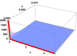
$R_{\mu\nu\rho\sigma}R^{\mu\nu\rho\sigma}\left(y,\alpha^{\prime}\right)$                                                 $b\left(y,\alpha^{\prime}\right)$

Figure 1: The figures display $R_{\mu\nu\rho\sigma}R^{\mu\nu\rho\sigma}\left(y,\alpha^{\prime}\right)$ and $b\left(y,\alpha^{\prime}\right)$, with the assumption $C=1$. The red lines represent the singular solutions $R_{\mu\nu\rho\sigma}R^{\mu\nu\rho\sigma}\left(y,0\right)$ and $b\left(y,0\right)$ obtained from (2.20). The singularities are located at $y=0$ and $\alpha^{\prime}=0$.

4 Conclusion

In this paper, we have successfully calculated the non-perturbative and non-singular solution for the Hohm-Zwiebach action, considered the presence of a non-trivial Kalb-Ramond field. In order to calculate the matrix differential equations, we transformed the infinite summation of matrices into a simple trace of a matrix, enabled us to solve the matrix differential equations. As a result, we obtained regular solutions for all the fields, including the spacetime metric. This implies that the naked singularity of the extremal black string can be eliminated by the $\alpha^{\prime}$ corrections. In our future work, we plan to study the following aspects:

• Extension to anisotropic backgrounds: In this study, we focused on the isotropic background. However, it would be interesting to investigate the anisotropic Hohm-Zwiebach action. It implies that we need to consider the multitrace terms in the Hohm-Zwiebach action and refine our method accordingly.

• Application to BTZ black hole: The BTZ black hole solution in string theory also requires a non-trivial Kalb-Ramond field. Therefore, if we aim to address the curvature singularity in the BTZ black hole, it is crucial to incorporate the Kalb-Ramond field in the Hohm-Zwiebach action.

By addressing these directions, we can further broaden our understanding of non-perturbative solutions and their implications for resolving singularities in black hole spacetimes.

Acknowledgements We are very grateful to Xin Li, Peng Wang, Houwen Wu and Haitang Yang for many illuminating discussions and suggestions. This work is supported in part by NSFC (Grant No. 12105031), and the Postdoctoral Science Foundation of Chongqing (Grant No. cstc2021jcyj-bshX0227).

References

[1]
O. Hohm and B. Zwiebach, “T-duality Constraints on Higher Derivatives Revisited,” JHEP 1604, 101 (2016) doi:10.1007/JHEP04(2016)101 [arXiv:1510.00005 [hep-th]].
[2]
O. Hohm and B. Zwiebach, “Non-perturbative de Sitter vacua via corrections,” Int. J. Mod. Phys. D 28, no.14, 1943002 (2019) doi:10.1142/S0218271819430028 [arXiv:1905.06583 [hep-th]].
[3]
O. Hohm and B. Zwiebach, “Duality invariant cosmology to all orders in ’,” Phys. Rev. D 100, no.12, 126011 (2019) doi:10.1103/PhysRevD.100.126011 [arXiv:1905.06963 [hep-th]].
[4]
A. Sen, “O(d) x O(d) symmetry of the space of cosmological solutions in string theory, scale factor duality and two-dimensional black holes,” Phys. Lett. B 271, 295 (1991). doi:10.1016/0370-2693(91)90090-D
[5]
A. Sen, “Twisted black p-brane solutions in string theory,” Phys. Lett. B 274, 34 (1992) doi:10.1016/0370-2693(92)90300-S [hep-th/9108011].
[6]
G. Veneziano, “Scale factor duality for classical and quantum strings,” Phys. Lett. B 265, 287 (1991). doi:10.1016/0370-2693(91)90055-U
[7]
K. A. Meissner and G. Veneziano, “Symmetries of cosmological superstring vacua,” Phys. Lett. B 267, 33 (1991). doi:10.1016/0370-2693(91)90520-Z
[8]
K. A. Meissner, “Symmetries of higher order string gravity actions,” Phys. Lett. B 392, 298 (1997) doi:10.1016/S0370-2693(96)01556-0 [hep-th/9610131].
[9]
P. Wang, H. Wu, H. Yang and S. Ying, “Non-singular string cosmology via corrections,” JHEP 1910, 263 (2019) doi:10.1007/JHEP10(2019)263 [arXiv:1909.00830 [hep-th]].
[10]
P. Wang, H. Wu, H. Yang and S. Ying, “Construct corrected or loop corrected solutions without curvature singularities,” JHEP 01, 164 (2020) doi:10.1007/JHEP01(2020)164 [arXiv:1910.05808 [hep-th]].
[11]
P. Wang, H. Wu and H. Yang, “Are nonperturbative AdS vacua possible in bosonic string theory?,” Phys. Rev. D 100, no. 4, 046016 (2019) doi:10.1103/PhysRevD.100.046016 [arXiv:1906.09650 [hep-th]].
[12] P. Wang, H. Wu, H. Yang and S. Ying, “Derive Lovelock Gravity from String Theory in Cosmological Background,” JHEP 05, 218 (2021) doi:10.1007/JHEP05(2021)218 [arXiv:2012.13312 [hep-th]].
[13] M. Gasperini and G. Veneziano, “Non-singular pre-big bang scenarios from all-order corrections,” [arXiv:2305.00222 [hep-th]].
[14] L. Song and D. Chen, “Two non-perturbative corrected or loop corrected string cosmological solutions,” [arXiv:2306.07031 [hep-th]].
[15] S. Ying, “Two-dimensional regular string black hole via complete corrections,” [arXiv:2212.03808 [hep-th]]. accepted by Eur.Phys.J.C
[16] S. Ying, “Three dimensional regular black string via loop corrections,” JHEP 03, 044 (2023) doi:10.1007/JHEP03(2023)044 [arXiv:2212.14785 [hep-th]].
[17] T. Codina, O. Hohm and B. Zwiebach, “2D Black Holes, Bianchi I Cosmologies, and ,” [arXiv:2304.06763 [hep-th]].
[18] S. Ying, “Two-dimensional regular string black hole in different gauges,” [arXiv:2306.17244 [hep-th]].
[19] H. Bernardo, P. R. Chouha and G. Franzmann, “Kalb-Ramond backgrounds in ’-complete cosmology,” JHEP 09, 109 (2021) doi:10.1007/JHEP09(2021)109 [arXiv:2104.15131 [hep-th]].
[20] T. Codina, O. Hohm and D. Marques, “General string cosmologies at order ’3,” Phys. Rev. D 104, no.10, 106007 (2021) doi:10.1103/PhysRevD.104.106007 [arXiv:2107.00053 [hep-th]].
[21]
G. Mandal, A. M. Sengupta and S. R. Wadia, “Classical solutions of two-dimensional string theory,” Mod. Phys. Lett. A 6, 1685-1692 (1991) doi:10.1142/S0217732391001822
[22]
J. H. Horne and G. T. Horowitz, “Exact black string solutions in three-dimensions,” Nucl. Phys. B 368, 444-462 (1992) doi:10.1016/0550-3213(92)90536-K [arXiv:hep-th/9108001 [hep-th]].
[23] A. Dabholkar, G. W. Gibbons, J. A. Harvey and F. Ruiz Ruiz, “Superstrings and Solitons,” Nucl. Phys. B 340, 33-55 (1990) doi:10.1016/0550-3213(90)90157-9