Monitoring the large-scale magnetic field of AD Leo with SPIRou, ESPaDOnS, and Narval

Abstract

Context. One clear manifestation of dynamo action on the Sun is the 22-yr magnetic cycle, exhibiting a polarity reversal and a periodic conversion between poloidal and toroidal fields. For M dwarfs, several authors claim evidence of activity cycles from photometry and analyses of spectroscopic indices, but no clear polarity reversal has been identified from spectropolarimetric observations. These stars are excellent laboratories to investigate dynamo-powered magnetic fields under different stellar interior conditions, that is partly or fully convective.

Aims. Our aim is to monitor the evolution of the large-scale field of AD Leo, which has shown hints of a secular evolution from past dedicated spectropolarimetric campaigns. This is of central interest to inform distinct dynamo theories, contextualise the evolution of the solar magnetic field, and explain the variety of magnetic field geometries observed in the past.

Methods. We analysed near-infrared spectropolarimetric observations of the active M dwarf AD Leo taken with SPIRou between 2019 and 2020 and archival optical data collected with ESPaDOnS and Narval between 2006 and 2019. We searched for long-term variability in the longitudinal field, the width of unpolarised Stokes profiles, the unsigned magnetic flux derived from Zeeman broadening, and the geometry of the large-scale magnetic field using both Zeeman-Doppler imaging and principal component analysis.

Results. We found evidence of a long-term evolution of the magnetic field, featuring a decrease in axisymmetry (from 99% to 60%). This is accompanied by a weakening of the longitudinal field ($-$300 to $-$50 G) and a correlated increase in the unsigned magnetic flux (2.8 to 3.6 kG). Likewise, the width of the mean profile computed with selected near-infrared lines manifests a long-term evolution corresponding to field strength changes over the full time series, but does not exhibit modulation with the stellar rotation of AD Leo in individual epochs.

Conclusions. The large-scale magnetic field of AD Leo manifested first hints of a polarity reversal in late 2020 in the form of a substantially increased dipole obliquity, while the topology remained predominantly poloidal and dipolar for 14 yr. This suggests that low-mass M dwarfs with a dipole-dominated magnetic field can undergo magnetic cycles.

1 Introduction

Studying stellar surface magnetic fields yields relevant insights into the internal structure of stars, as well as their essential role in stellar formation, evolution, and activity (Donati & Landstreet, 2009). For cool stars, monitoring secular changes of the field’s configuration provides useful feedback on the dynamo processes operating in the stellar interior and constraints on stellar wind models. The latter is fundamental to understanding atmospheric hydrodynamic escape of embedded planets since magnetic cycles modulate the star’s activity level and thus its radiation output (Vidotto & Cleary, 2020; Hazra et al., 2020).

The Sun is an important benchmark in this context: its long-term monitoring revealed a periodic variation in sunspot number, size, and latitude (Schwabe, 1844; Maunder, 1904; Hathaway, 2010), and a polarity reversal of the large-scale magnetic field over a timescale of 11 yr (Hale et al., 1919). The proposed mechanism to reproduce these phenomena theoretically is the $\alpha\Omega$ dynamo (Parker, 1955; Charbonneau, 2010), namely the combination of differential rotation and cyclonic turbulence at the interface between the radiative and convective zones, known as tachocline. A different model is the Babcock-Leighton mechanism, which describes the conversion from a toroidal to poloidal field via a poleward migration of bipolar magnetic regions (Babcock, 1961; Leighton, 1969). However, there is still no model that can account for all the solar magnetic processes (Petrovay, 2020).

For other stars, magnetic field measurements can be performed with two complementary approaches (Morin, 2012; Reiners, 2012). One is to model the Zeeman splitting in individual unpolarised spectral lines and estimate the total unsigned magnetic field, which is insensitive to polarity cancellation. The other is to apply tomographic techniques that use the polarisation properties of the Zeeman-split components to recover the orientation of the local field. In addition to these well-established methods, Lehmann & Donati (2022) show that fundamental properties of the large-scale field topology can be derived directly from the circularly polarised Stokes $V$ time series using principal component analysis (PCA), without prior assumptions. This method allows us to qualitatively infer the predominant component of the field topology, as well as its complexity, axisymmetry, and evolution. Altogether, these observational constraints guide dynamo theories to a comprehensive description of the magnetic field generation and dynamic nature in the form of magnetic cycles (Reiners et al., 2010; Gregory et al., 2012; See et al., 2016).

Over the last three decades, Zeeman-Doppler imaging (ZDI, Semel 1989; Donati & Brown 1997) has been applied to reconstruct the poloidal and toroidal components of stellar magnetic fields, providing evidence of a wide variety of the large-scale magnetic topologies (e.g., Morin et al., 2016). Among rapidly rotating cool stars, the partly convective ones with masses above 0.5 M_⊙ tend to have moderate, predominantly toroidal large-scale fields generally featuring a non-axisymmetric poloidal component (Petit et al., 2008; Donati et al., 2008a; See et al., 2015). Those with masses between 0.2 M_⊙ and 0.5 M_⊙ – close to the fully convective boundary at 0.35 M_⊙ (Chabrier & Baraffe, 1997) – generate stronger large-scale magnetic fields, dominated by a poloidal and axisymmetric component. For fully convective stars with M$<$0.2 M_⊙, spectropolarimetric analyses have revealed a dichotomy of field geometries: either strong, mostly axisymmetric dipole-dominated or weak, non-axisymmetric multipole-dominated large-scale fields are observed (Morin et al., 2010). The latter findings could be understood either as a manifestation of dynamo bistability (Morin et al., 2011; Gastine et al., 2013), that is two dynamo branches that coexist over a range of stellar rotation periods and masses, or of long magnetic cycles, implying that different topologies correspond to different phases of the cycle (Kitchatinov et al., 2014). Yet, no firm conclusion has been reached. In parallel, studies relying on the analysis of unpolarised spectra have shown that the average (unsigned) surface magnetic field of cool stars follows a classical rotation-activity relation including a non-saturated and a saturated (or quasi-saturated) regime, without a simple relation with the large-scale magnetic geometry (Reiners & Basri, 2009; Shulyak et al., 2019; Kochukhov, 2021; Reiners et al., 2022). Similarly, recent dynamo simulations conducted by, for instance, Zaire et al. (2022) confirm that the influence of rotation on convective motions alone could not explain the observed variety of magnetic geometry. Only in the case of fully convective very fast rotators, Shulyak et al. (2017) found that the strongest average fields were measured for stars with large-scale dipole-dominated fields. Kochukhov (2021) show that the fraction of magnetic energy contained in the large-scale field component is also the highest for these stars.

Cyclic trends for Sun-like stars were found via photometric and chromospheric activity (i.e. Ca II H&K lines) monitoring, and timescales shorter (e.g., 120 d for $\tau$ Boo, Mittag et al. 2017) or longer ($\simeq$ 20 yr for HD 1835; Boro Saikia et al. 2018) than the solar magnetic cycle were reported (Wilson, 1968; Baliunas et al., 1995; Boro Saikia et al., 2018). Moreover, polarity flips of the large-scale field were detected for a handful of stars based on optical spectropolarimetric observations (Donati et al., 2008b; Petit et al., 2009; Fares et al., 2009; Morgenthaler et al., 2011; Boro Saikia et al., 2016; Rosén et al., 2016; Jeffers et al., 2018; Boro Saikia et al., 2022; Jeffers et al., 2022). For M dwarfs, numerous studies relying on photometry and spectroscopic indices claimed evidence of activity cycles (e.g., Gomes da Silva et al., 2012; Robertson et al., 2013; Mignon et al., 2023), and radio observations suggest the occurrence of polarity reversal at the end of the main sequence (Route, 2016), but no polarity reversal has been directly observed with spectropolarimetry so far. This motivates long-term spectropolarimetric surveys, to reveal secular changes in the field topology and shed more light on the dynamo processes in action.

A well-known active M dwarf is AD Leo (GJ 388), whose mass (0.42 M_⊙) falls at the boundary between the domains where toroidal- and dipole-dominated magnetic topologies have previously been identified, and thus represents an interesting laboratory to study stellar dynamos. Morin et al. (2008b) analysed the large-scale magnetic field from spectropolarimetric data sets collected with Narval at Télescope Bernard-Lyot in 2007 and 2008 and reported a stable, axisymmetric, dipole-dominated geometry. Later, Lavail et al. (2018) examined data collected with ESPaDOnS at Canada-France-Hawaii Telescope (CFHT) from 2012 and 2016, and showed an evolution of the field in the form of a global weakening (about 20%) and small-scale enhancement. The latter was quantitatively expressed by a decrease in the magnetic filling factor (from 13% to 7%), meaning that the field was more intense on local scales. No polarity reversal was reported on AD Leo (Lavail et al., 2018). The large-scale magnetic topology has remained stable since spectropolarimetric observations of AD Leo have been initiated (2007–2016): dominated by a strong axial dipole, the visible pole corresponding to negative radial field (magnetic field vector directed towards the star).

Here, we extend the magnetic analysis of AD Leo using both new optical ESPaDOnS observations collected in 2019 and near-infrared spectropolarimetric time series collected with SPIRou at CFHT in 2019 and 2020 under the SPIRou Legacy Survey (SLS), which adds to the previous optical data sets collected with ESPaDOnS and Narval between 2006 and 2016. The aim is to apply distinct techniques to search for long-term variations that may or may not resemble the solar behaviour.

The paper is structured as follows: in Sec. 2 we describe the observations performed in the near-infrared and optical domains, in Sec. 3 we outline the temporal analysis of the longitudinal magnetic field, the Full-Width at Half Maximum (FWHM) of the Stokes $I$ profile, and the total magnetic flux inferred from Zeeman broadening modelling. Then, we describe the magnetic geometry reconstructions by means of ZDI and PCA. In Sec. 4 we discuss the wavelength dependence of magnetic field measurements and in Sec. 5 we present our conclusions.

2 Observations

AD Leo is an M3.5 dwarf with a $V$ and $H$ band magnitude of 9.52 and 4.84, respectively (Zacharias et al., 2013), at a distance of 4.9651$\pm$0.0007 pc (Gaia Collaboration et al., 2021). Its age was estimated to be within 25 and 300 Myr by Shkolnik et al. (2009). AD Leo has a rotation period of 2.23 days (Morin et al., 2008b; Carmona et al., 2023) and an inclination $i=20^{\circ}$, implying an almost pole-on view (Morin et al., 2008b). Its high activity level is seen in frequent flares (Muheki et al., 2020; Namekata et al., 2020) and quantified by an X-ray-to-bolometric luminosity ratio ($\log(\mathrm{L}_{\mathrm{X}}/\mathrm{L}_{\mathrm{bol}})$) of -3.62 (Wright et al., 2011) and a mean CaII H&K index ($\mathrm{logR^{\prime}}_{\mathrm{HK}}$) of -4.00 (Boro Saikia et al., 2018).

AD Leo’s mass is 0.42 $M_{\odot}$ (Mann et al., 2015; Cristofari et al., 2023), which places it above the theoretical fully convective boundary at 0.35 $M_{\odot}$ (Chabrier & Baraffe, 1997). The latter value is in agreement with observations, as it has been invoked to explain the dearth of stars with $M_{G}\sim$10.2, known as Gaia magnitude gap (Feiden et al., 2021). However, it is not an absolute limit: age (Maeder & Meynet, 2000) and metallicity affect the depth of the convective envelope (van Saders & Pinsonneault, 2012; Tanner et al., 2013), and the presence of strong magnetic fields quenches convection and could push the theoretical boundary towards later spectral type (Mullan & MacDonald, 2001).

Figure 1: Example Stokes profiles for AD Leo for the 9th December 2019 observation collected with SPIRou. From the top: Stokes $I$ profile (unpolarised); Stokes $V$ profile (circularly polarised) with a clear Zeeman signature of S/N = 6 500, and Null $N$ profile, used for quality check of the Stokes profiles (Donati et al., 1997; Bagnulo et al., 2009). The LSD profiles were obtained using a mask containing 838 lines. In all panels, the units are relative to the unpolarised continuum.

2.1 Near-infrared

A total of 77 spectropolarimetric observations in the near-infrared were collected with the SpectroPolarimètre InfraRouge (SPIRou) within the SLS. SPIRou is a stabilised high-resolution near-infrared spectropolarimeter (Donati et al., 2020) mounted on the 3.6 m CFHT atop Maunakea, Hawaii. It provides a full coverage of the near-infrared spectrum from 0.96 to $2\mu$m at a spectral resolving power of $R\sim 70,000$. Optimal extraction of SPIRou spectra was carried out with A PipelinE to Reduce Observations (APERO v0.6.132), a fully automatic reduction package installed at CFHT (Cook et al., 2022). The same data set was used in Carmona et al. (2023) to perform a velocimetric study and reject the hypothesis of a planetary companion by Tuomi et al. (2018) in favour of activity-induced variations, in agreement with Carleo et al. (2020).

Observations were performed in circular polarisation mode between February 2019 and June 2020, spanning 482 days in total; the journal of observations is available in Table LABEL:tab:log. The mean airmass is 1.32 and the signal-to-noise ratio (S/N) at $1,650$ nm per spectral element ranges from 68 to 218, with an average of 168. We applied least-squares deconvolution (LSD) to atomic spectral lines to derive averaged-line Stokes $I$ (unpolarised) and $V$ (circularly polarised) profiles (Donati et al., 1997; Kochukhov et al., 2010). This numerical technique assumes the spectrum to be the convolution between a mean line profile and a line mask, that is to say a series of Dirac delta functions centred at each absorption line in the stellar spectrum, with corresponding depths and Landé factors (i.e. sensitivities to the Zeeman effect at a given wavelength). The output mean line profile gathers the information of thousands of spectral lines and, because of the consequent high S/N, enables the extraction of polarimetric information from the spectrum. The adopted line mask was generated using the Vienna Atomic Line Database (VALD, Ryabchikova et al., 2015) and a MARCS atmosphere model (Gustafsson et al., 2008) with $T_{\mathrm{eff}}=3,500$ K, $\log g=$ 5.0 [cm s^-2] and $v_{\mathrm{micro}}=$ 1 km s^-1. It contains $1,400$ atomic lines between 950–$2,600$ nm and with known Landé factor (ranging from 0 to 3) and with depth larger than 3 % of the continuum level.

We discarded six observations in February 2019 since one optical component of the instrument was not working nominally, one observation in November 2019 because likely affected by a flare (the corresponding radial velocity is $>$8 sigma lower than the bulk of the measurements) and two observations in 2020 as they led to noisier (by a factor of 10) LSD profiles. Therefore, the data set analysed in this work comprises 68 polarimetric sequences, whose characteristics are reported in Table LABEL:tab:log.

The near-infrared observations were performed monthly between 2019 and 2020, except for two gaps of approximately two and three months. There is also a gap of 1.5 month between the end of 2019 and beginning of 2020. We thus split the time series in four epochs to maintain coherency of magnetic activity over short time scales and for clearer visualisation: 2019a (15th April 2019 to 21st June 2019, i.e. 2019.29 to 2019.47), 2019b (16th October 2019 to 12th December 2019, i.e. 2019.79 to 2019.95) 2020a (26th January 2020 to 12th March 2020, i.e. 2020.07 to 2020.19), and 2020b (8th May 2020 to 10th June 2020, i.e. 2020.35 to 2020.44).

The near-infrared domain covered by SPIRou is polluted by strong and wide telluric bands due to Earth’s atmospheric absorption. Their contribution to the stellar spectra is corrected using a telluric transmission model (which is built from observations of standard stars since the start of SPIRou operations, and using Transmissions of the AtmosPhere for AStromomical data (TAPAS) atmospheric model Bertaux et al. 2014) and a PCA method implemented in the APERO pipeline (Artigau et al., 2014). To account for potential residuals in the telluric correction, we ignored the following intervals of the spectrum when computing the LSD profiles: [950, 979], [1116, 1163], [1331, 1490], [1790, 1985], [1995,2029], [2250, 2500] nm. These intervals correspond to H₂O absorption regions, with transmission typically smaller than 40%. We assessed whether removing these telluric intervals optimises the quality of the Stokes $V$ profiles. In a first test, we searched for stellar absorption lines deeper than 75 % of the continuum level and within $\pm 100$ km s^-1 from telluric lines included in the transmission model of APERO. This approach allowed us to identify stellar lines that are contaminated by the telluric lines throughout the year. When the telluric-affected spectral lines were removed, no significant improvement was reported in the final LSD profiles, indicating a robust telluric correction as already reported in (Carmona et al., 2023). In a second test, we extended the intervals by 25 and 50 nm or reduced them by 10 nm and noticed an increment of the noise level in LSD profiles up to 20 %, so we proceeded with the previous intervals.

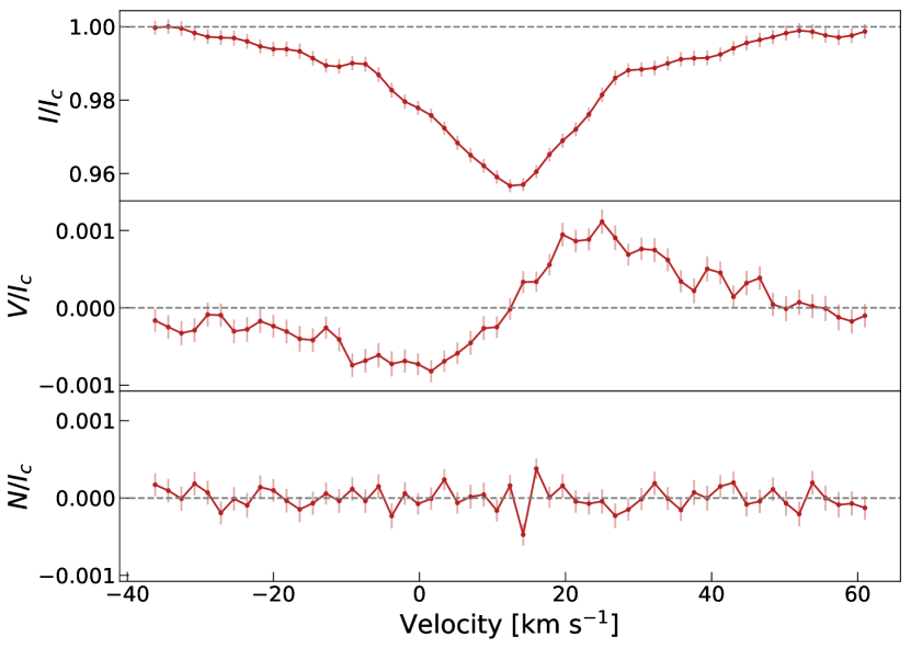
Accounting for the ignored telluric intervals, the number of spectral lines used in LSD is 838. We show the LSD Stokes profiles for one example observation in Fig. 1. The average noise level in Stokes $V$ for the entire time series is $1.6\cdot 10^{-4}$ relative to the unpolarised continuum, similar to the optical domain (Morin et al., 2008b). We also note that the profiles are broader than in the optical by more than $10$ km s^-1, owing to a stronger Zeeman effect in the near-infrared domain (Zeeman, 1897).

2.2 Optical

For most of the analyses presented here, we considered all archival observations collected with ESPaDOnS and Narval, and studied previously in Morin et al. (2008b) and Lavail et al. (2018). We also included six new observations taken in November 2019 (from 2019.87 to 2019.89) with ESPaDOnS for CFHT programme 19BC06, PI A. Lavail (reported in Table LABEL:tab:log_opt). They are contemporaneous to the SPIRou ones for the same period, hence enabling us to study the dependence of the measured magnetic field strength on the wavelength domain employed (see Sec. 4).

ESPaDOnS is the optical spectropolarimeter on the 3.6 m CFHT located atop Mauna Kea in Hawaii, and Narval is the twin instrument on the 2 m TBL at the Pic du Midi Observatory in France (Donati, 2003). The data reduction was performed with the LIBRE-ESPRIT pipeline (Donati et al., 1997), and the reduced spectra were retrieved from the PolarBase archive (Petit et al., 2014).

The LSD profiles were computed similar to the near-infrared, but using an optical VALD mask containing 3330 lines in range 350-1080 nm and with depths larger than 40% the continuum level, similar to Morin et al. (2008b); Bellotti et al. (2022). The number of lines used is 3240 and accounts for the removal of the following wavelength intervals, which are affected by telluric lines or in the vicinity of H$\alpha$: [627,632], [655.5,657], [686,697], [716,734], [759,770], [813,835], and [895,986] nm. For the 2019 observations, the average noise in Stokes $V$ is $3\cdot 10^{-4}$ relative to the unpolarised continuum.

In the next sections, the near-infrared and optical observations will be phased with the following ephemeris:

$$\mathrm{HJD}=2458588.7573+\mathrm{P}_{\mathrm{rot}}\cdot n_{\mathrm{cyc}}\text{ , }$$ (1)

where we used the first SPIRou observation taken in April 2019 as reference, P${}_{\mathrm{rot}}=$2.23 days is the stellar rotation period (Morin et al., 2008b), and $n_{\mathrm{cyc}}$ corresponds to the rotation cycle (see Table LABEL:tab:log).

3 Magnetic analysis

3.1 Longitudinal magnetic field

Figure 2: Temporal evolution of the longitudinal magnetic field (B_l). Top: full time series of measurements between 2006 and 2020 with ESPaDOnS, Narval and SPIRou. The shape of the data points corresponds to the wavelength domain, optical (circles) or near-infrared (pluses), and the colour to the epoch in which the observations were performed. Bottom: SPIRou time series split in four epochs phase-folded according to Eq. 1. The least-square sine fit corresponding to Eq. 3 (Stibbs, 1950), to assess the change in magnetic obliquity, is shown as dashed lines. The six ESPaDOnS observations taken in 2019 are plotted as pink circles.

Table 1: Best fit values of the polar field and obliquity of Eq. 3 obtained for optical and near-infrared epochs.

	2006	2007	2008	2012	2016	2019a	2019b	2020a	2020b
$B_{p}$ [G]	$-868\pm 20$	$-842\pm 21$	$-873\pm 15$	$-736\pm 19$	$-555\pm 10$	$-814\pm 17$	$-882\pm 22$	$-828\pm 55$	$-923\pm 70$
$\beta$ [∘]	$13\pm 6$	$12\pm 4$	$26\pm 1$	$7\pm 4$	$12\pm 1$	$3\pm 4$	$23\pm 2$	$37\pm 4$	$59\pm 2$

Table 2: Comparison of a constant line vs a sine fit for the FWHM phase variations.

Epoch	Mask	Mean	Mean Error	STD	RMSconst	$\chi^{2}_{r,\mathrm{const}}$	RMSsine	$\chi^{2}_{r,\mathrm{sine}}$
		[km s-1]	[km s-1]	[km s-1]	[km s-1]		[km s-1]
2019a	default	19	0.29	0.40	0.40	1.8	0.39	2.0
	g${}_{\mathrm{eff}}>1.2$	23	0.46	1.16	1.16	6.9	1.13	8.0
2019b	default	21	0.41	0.63	0.63	2.3	0.62	2.5
	g${}_{\mathrm{eff}}>1.2$	27	0.84	1.77	1.77	6.7	1.71	6.9
2020a	default	21	0.41	0.68	0.68	3.2	0.61	3.4
	g${}_{\mathrm{eff}}>1.2$	27	0.82	2.47	2.47	12.2	2.29	13.3
2020b	default	19	0.30	0.47	0.47	3.0	0.47	3.4
	g${}_{\mathrm{eff}}>1.2$	22	0.46	0.83	0.83	5.3	0.79	7.3

We measured the line-of-sight component of the magnetic field integrated over the stellar disk (B_l) for all the available observations, in optical (2006–2019) and near-infrared (2019–2020). Since B_l traces magnetic features present on the visible hemisphere, its temporal variations are modulated at the stellar rotation period and can be therefore used as a robust magnetic activity proxy (Folsom et al., 2016; Hébrard et al., 2016; Fouqué et al., 2023). Formally, it is computed as the first-order moment of Stokes V (Donati et al., 1997):

$$\mathrm{B}_{l}\;[G]=\frac{-2.14\cdot 10^{11}}{\lambda_{0}\mathrm{g}_{\mathrm{eff}}c}\frac{\int vV(v)dv}{\int(I_{c}-I)dv}\,,$$ (2)

where $\lambda_{0}$ and $\mathrm{g}_{\mathrm{eff}}$ are the normalisation wavelength and Landé factor of the LSD profiles, $I_{c}$ is the continuum level, $v$ is the radial velocity associated to a point in the spectral line profile in the star’s rest frame and $c$ the speed of light in vacuum. For the near-infrared and optical Stokes profiles, the normalisation wavelength and Landé factor are 1700 nm and 1.2144, and 700 nm and 1.1420, respectively. In accordance with the fact that near-infrared lines are broader than optical ones, the integration was carried out within $\pm$ 50 km s^-1 from line centre in the former case and $\pm$ 30 km s^-1 in the latter case, to include the absorption ranges of both Stokes $I$ and $V$ profiles.

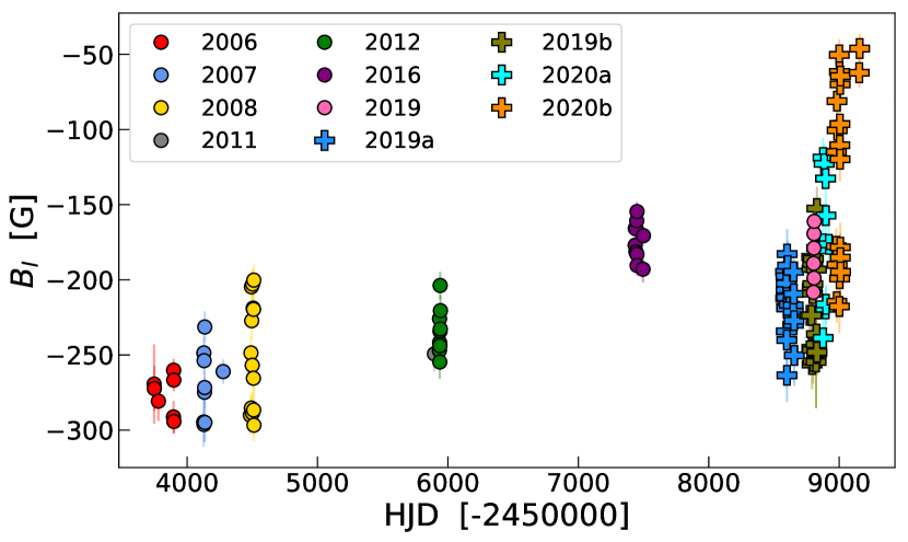
The list of measurements is reported in Table LABEL:tab:Bl_log. The values are of constant sign (negative), which is expected when observing one polarity of a dipole almost aligned with the stellar rotation axis over the entire stellar rotation, especially for a star observed nearly pole-on as AD Leo (Morin et al., 2008b; Lavail et al., 2018). The near-infrared measurements range between $-263$ and $-46$ G, with an average of $-179$ G and a median error bar of 15 G. The optical measurements range between $-297$ and $-155$ G, with an average of $-233$ G and a median error bar of 10 G. The lower error bar is likely due to the narrower velocity range over which the optical measurements are performed, since less noise is introduced in Eq. 2. A discussion about chromatic differences in the longitudinal field measurements is presented in Sec. 4.

We plot the temporal evolution of B_l in Fig. 2. In general, we note a secular weakening of the field strength over 14 yr, with an oscillation between 2016 and 2019 followed by a rapid decrease in strength (in absolute value). We also note that the intra-epoch dispersion increases for the last two epochs.

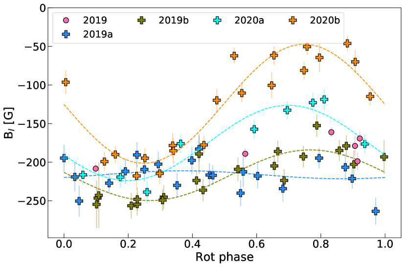
By phase-folding the near-infrared data at P_rot, we observe a systematic increase in the rotational modulation towards 2020b, meaning that the axisymmetry level of the field has likely decreased (see Fig. 2). For a first quantitative evaluation, we followed Stibbs (1950) and Preston (1967) to model the phase variations of the longitudinal field for a predominantly-dipolar magnetic configuration. Formally,

$$\mathrm{B}_{l}\;[G]=\frac{1}{20}\frac{15+\varepsilon}{3-\varepsilon}\mathrm{B}_{p}\left(\cos\beta\cos i+\sin\beta\sin i\cos(2\pi p)\right)\,,$$ (3)

with $\varepsilon$ the limb darkening coefficient (set to 0.3; Claret & Bloemen 2011), $p$ the rotational phase, B_p the longitudinal field of the dipole, $i$ the stellar inclination and $\beta$ the obliquity between magnetic and rotation axes. The results are listed in Table 1, for both near-infrared and optical time series for completeness. The six optical observations in November 2019 have poor coverage (three of them are clustered around phase 0.9) and lead to a less reliable sine fit. Nevertheless, they are compatible with the 2019b fit curve. These clues clearly indicate that the magnetic field of AD Leo is evolving, in agreement with Lavail et al. (2018), and demonstrate the interest of long-term spectropolarimetric monitoring of active M dwarf stars.

3.2 The mean line width

Figure 3: Phase variations of the FWHM, folded at a stellar rotation period of 2.23 days. The data sets are computed with the default (black), high-g_eff (yellow), and low-g_eff (purple) mask for three epochs: 2019a (top left), 2019b (top right), 2020a (bottom left), 2020b (bottom right). Although no evident rotational modulation is observed, we notice a long-term oscillation of the mean value in a similar way to the longitudinal field (absolute) values.

The width of near-infrared spectral lines of stars with intense fields and low equatorial velocity such as AD Leo ($v_{e}\sin(i)=$ 3 km s^-1; Morin et al. 2008b) are sensitive to the Zeeman effect, given its proportionality to wavelength, field strength, and Landé factor. The rotationally-modulated line broadening correlates with the azimuthal distribution of the unsigned small-scale magnetic flux, a useful diagnostic for stellar activity radial velocity contamination, as shown for the Sun by Haywood et al. (2022). In this context, Klein et al. (2021) adopted a selection of magnetically sensitive lines for the young star AU Mic and saw a correspondence in the variations of RV and FWHM of the Stokes $I$ profiles at the stellar rotation period. This confirmed the sensitivity of the FWHM to the distortions induced by magnetic regions on the stellar surface.

Here, we proceeded analogously in an attempt to connect modulations of the FWHM with variations of the large-scale field. We applied LSD on the near-infrared data using a mask of 417 lines characterised by g${}_{\mathrm{eff}}>1.2$, following Bellotti et al. (2022). The near-infrared time series was divided in four epochs as in Sec. 3.1 for consistency.

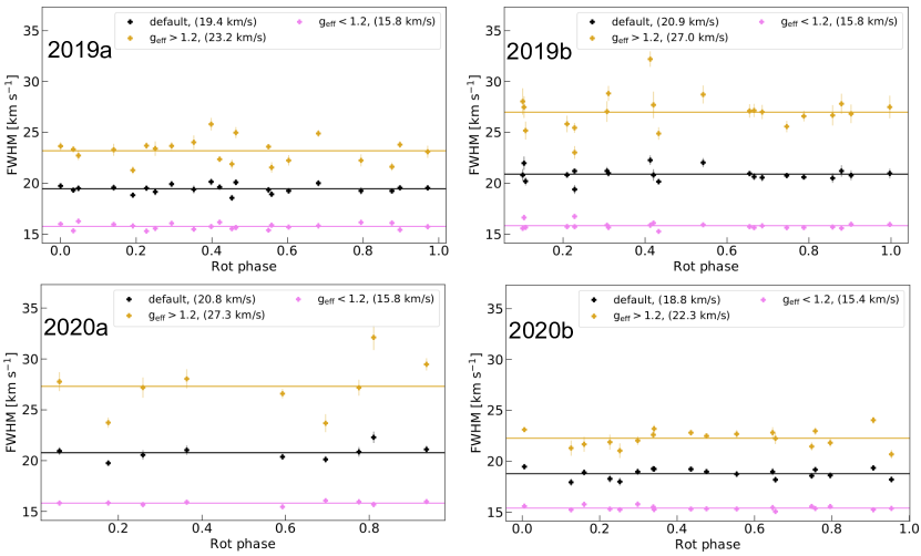
In Table 2, we compare the phase variations of the FWHM when adopting the default and high-g_eff masks, and we inspect whether they are more compatible with a sine fit or a constant fit equal to the mean of the data set. In all cases, there is no clear rotational modulation of the data points, as the sine fit does not provide a better description (i.e. lower $\chi^{2}_{r}$) of the variations than the constant fit. This is confirmed by a quick inspection of the periodogram applied to the FWHM data for each individual epoch. The $\chi^{2}_{r}$ increase when using a sine model rather than a constant is not statistically significant. The observed variations are attributable to dispersion, as illustrated in Fig. 3. We observed that the FWHM is systematically larger in all epochs for the high-g_eff mask, as expected given the linear dependence of Zeeman effect to g_eff, and the dispersion is between 1.8 and 3.0 times larger. The lack of rotational modulation prevents us from searching for correlations with other quantities such as RV and B_l as done in Klein et al. (2021).

From Fig. 3, we also noticed an evident long-term evolution of the mean FWHM. Such evolution has a moderate correlation (Pearson $R$ coefficient of 0.5) with the variations of the mean B_l for the same epochs, meaning that the FWHM is a reasonable proxy to trace long-term evolution of the field. This is consistent with the recent Donati et al. (2023) analysis analysis of AU Mic. When using the default mask, the mean FWHM oscillated from 19 km s^-1 in 2019a to 21 km s^-1 in 2019b and 2020a, and back to 19 km s^-1 in 2020b. As expected, such oscillation is enhanced when considering the magnetically sensitive lines and goes from 23 km s^-1 in 2019a to 27 km s^-1 in 2019b and 2020a, and back to 22 km s^-1 in 2020b. We performed the same analysis with low-Landé factor lines (i.e. g${}_{\mathrm{eff}}<1.2$ and 406 lines) and noticed no appreciable variation of the mean FWHM, since it remained stable at $\sim$15 km s^-1. A view of the Stokes $I$ profiles computed with the three different line lists can be found in Appendix A.

The FWHM analysis was also carried out on the ESPaDOnS and Narval data between 2006 and 2019. When using low-g_eff lines, the mean width of Stokes $I$ is reasonably stable around 9.7 km s^-1, stressing their potential for precise radial velocity measurements. The full (high-g_eff) mask yields a mean value at 10 km s^-1 (12 km s^-1) between 2006 and 2012, which then increases to 11 km s^-1 (13 km s^-1) in 2016 and 2019. Such long-term evolution is only moderate compared to the one seen in the near-infrared time series. The entire evolution is illustrated in Fig. 4.

Figure 4: Secular evolution of the epoch-averaged FWHM of Stokes $I$. The scale on the left refers to optical data, while on the right to the near-infrared, and the colours indicate the use of different masks similar to Fig. 3. Both optical (circles) and near-infrared (pluses) observations feature a long-term variation, which is enhanced (quenched) when using magnetically sensitive (insensitive) lines. We note that the optical data point of 2019 falls behind the near-infrared ones when using magnetically sensitive lines.

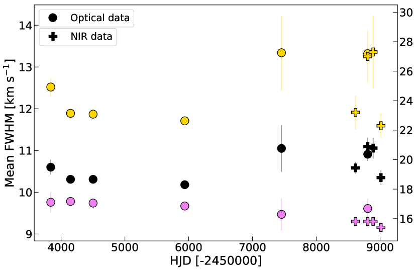
The difference between the mean FWHM of low-g_eff lines in optical ($\sim$9.5 km s^-1) and near-infrared ($\sim$16 km s^-1) can be attributed to lines that have non-zero Landé factor. Indeed, the quadratic differential broadening between the two domains is $11.4$ km s^-1, corresponding to a total magnetic field of 2.5 kG for a line at 1700 nm with g_eff=0.96 (the normalisation values of the low-g_eff mask). Although we assumed that the Zeeman effect for low-g_eff lines is negligible in the optical with this exercise, the inferred value of total magnetic field is reasonably consistent with what is reported in the literature (Saar, 1994; Shulyak et al., 2017, 2019), indicating that the magnetic field accounts mostly for the difference in width between optical and near-infrared low-g_eff lines.

Our analysis confirms that the FWHM is capable of tracing secular changes in the total, unsigned magnetic field, which could be used to better understand stellar activity jitter. Activity-mitigating techniques would benefit from this information even for low-inclination stars such as AD Leo, for which the phase modulation of the radial velocity jitter is more difficult to constrain. At the same time, the analysis highlights the presence of short-term variability producing scatter and that is not rotationally modulated.

Figure 5: Example fits including Zeeman broadening resulting from the MCMC-based approach of radiative transfer modelling. Top: ESPaDOnS observation from 24 Febuary 2016. Bottom: SPIRou observation from 3 November 2020. The panels have the same wavelength scale with minor ticks at 0.1 nm.

3.3 Modelling Zeeman broadening

To further investigate the small-scale magnetic field of AD Leo we conducted a Zeeman broadening analysis. For this analysis we used the full set of new and archival data, both in the near-infrared from SPIRou and in the optical from ESPaDOnS and Narval. All the data sets require a telluric correction, since telluric lines are present in much of the SPIRou wavelength range, and the red end of the ESPaDOnS and Narval range. For the SPIRou data we relied on the telluric correction from the APERO pipeline (Sec 2.1, Cook et al. 2022 for more detail). For the ESPaDOnS and Narval data, we made a telluric correction using the molecfit pipeline, originally designed for handling spectra from ESO instruments (Smette et al., 2015; Kausch et al., 2015). molecfit retrieves weather conditions and other relevant information at the time of observation and models the atmosphere in the line of sight. It performs radiative transfer and iteratively models the telluric component in the input spectrum while also fitting the continuum and the wavelength scale of the spectrum. It finally corrects telluric lines and provides a telluric-corrected output spectrum. After telluric correction the spectra were re-normalised in the regions of interest using a low order polynomial fit through carefully selected continuum regions. A few ESPaDOnS and Narval spectra were affected by fringing effects, hence we adopted a higher-order polynomial fit to normalise to a flatter continuum. Finally, we discarded any observations where the telluric correction left a noticeable residual feature that was blended with the stellar lines of interest.

To characterise the magnetic field, we fitted synthetic spectra to the observed Stokes $I$ spectra, incorporating both the Zeeman broadening and intensification effects. Synthetic spectra were calculated with Zeeman (Landstreet, 1988; Wade et al., 2001; Folsom et al., 2016), using model atmospheres from marcs (Gustafsson et al., 2008). Zeeman performs polarised radiative transfer including the Zeeman effect. However, a major limitation for M-dwarfs is that the programme does not currently include molecular lines, which are not typically used in Zeeman broadening analyses. Weak molecular lines are blended with many atomic lines in the spectra of M-dwarfs. With careful attention we identified a set of atomic lines suitable for AD Leo, with no evident distortion in the line shape by molecular blends. Thus the systematic error from this limitation is expected to be negligible, but the inclusion of molecular lines in the future would substantially simplify the selection of lines for Zeeman broadening analyses, as shown in the recent work of Cristofari et al. (2023) and previously applied to AD Leo by Shulyak et al. (2014, 2017). To check the validity of the analysis presented here, a second analysis of the ESPaDOnS and Narval spectra was carried out with the SYNMAST code (Kochukhov et al., 2010). The analyses used nearly the same set of Ti i lines, and the results we obtained were consistent within uncertainty.

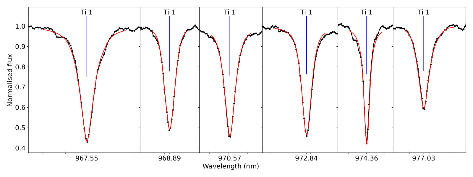
For the ESPaDOnS and Narval observations, we used the Ti i lines at 9675.54 Å (g${}_{\mathrm{eff}}=1.35$), 9688.87 Å (g${}_{\mathrm{eff}}=1.50$), 9705.66 Å (g${}_{\mathrm{eff}}=1.26$), 9728.40 Å (g${}_{\mathrm{eff}}=1.00$), 9743.61 Å (g${}_{\mathrm{eff}}=0.00$), and 9770.30 Å (g${}_{\mathrm{eff}}=1.55$). These lines have been used extensively for Zeeman broadening analysis (e.g., Kochukhov & Lavail, 2017; Hill et al., 2019; Kochukhov, 2021, and references therein) and have reliable oscillator strengths and Landé factors in VALD. These lines have relatively weak telluric blending, very little molecular blending, and a wide range of effective Landé factors.

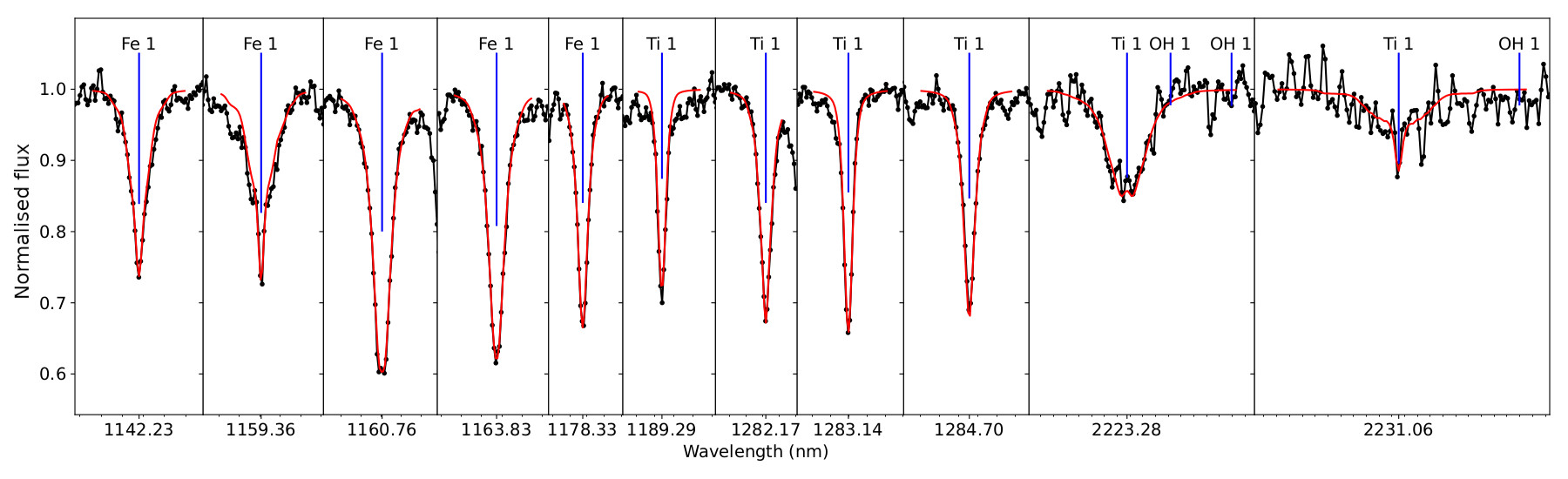
For the SPIRou observations, we selected a set of lines using similar criteria, but also avoided lines with large pressure broadened wings, since small errors in the pressure broadening could cause larger errors in the Zeeman broadening estimation. In order to maximise the range of available effective Landé factors we used the Fe i lines at 11422.32 Å  (g${}_{\mathrm{eff}}=1.98$), 11593.59 Å  (g${}_{\mathrm{eff}}=2.50$), 11607.57 Å  (g${}_{\mathrm{eff}}=1.66$), 11638.26 Å  (g${}_{\mathrm{eff}}=1.58$), and 11783.26 Å  (g${}_{\mathrm{eff}}=1.14$) and the Ti i lines at 11892.88 Å  (g${}_{\mathrm{eff}}=0.75$), 12821.67 Å  (g${}_{\mathrm{eff}}=1.26$), 12831.44 Å  (g${}_{\mathrm{eff}}=0.67$), 12847.03 Å  (g${}_{\mathrm{eff}}=1.08$), 22232.84 Å  (g${}_{\mathrm{eff}}=1.66$), and 22310.61 Å  (g${}_{\mathrm{eff}}=2.50$). This provides multiple lines with both high and low effective Landé factors, but uses lines from two different ions, which we compensated for by using the Ti and Fe abundances as independent free parameters in our analysis. There are a few other Ti i lines near 22000 Å with large effective Landé factors, but there is a relatively severe blending by many weak molecular lines in this region, hence we did not include these lines. Line data were extracted from VALD. In these line lists, experimental oscillator strengths for Ti i lines were from Lawler et al. (2013) (consistent with Blackwell-Whitehead et al., 2006), except for 22232.84 Å from Blackwell-Whitehead et al. (2006), and a theoretical value for 22310.61 Å from the compilation of R. L. Kurucz. Oscillator strengths for the Fe i lines were taken from O’Brian et al. (1991).

The total magnetic field was modelled with a grid of field strengths and filling factors for the fraction of the surface area with the corresponding field strength (e.g. Johns-Krull et al., 1999). A uniform radial orientation was assumed for the magnetic field, since Stokes $I$ spectra have little sensitivity to magnetic field orientation. This is also a reasonable assumption given the magnetic field maps reconstructed in Sec. 3.4. For the optical spectra, we adopted magnetic fields of 0, 2, 4, 6, 8, and 10 kG, and derived their filling factors. For the SPIRou spectra, we used a finer grid of 1 kG from 0 to 10 kG, since the sensitivity to Zeeman effect is larger at longer wavelengths, and a finer grid is needed to produce smooth line profiles.

To derive the magnetic filling factors we applied an MCMC-based approach, using the emcee package (Foreman-Mackey et al., 2013) integrated with Zeeman. The filling factors for $B>0$ were treated as free parameters, with the filling factor for $B=0$ ($f_{B=0}$) calculated from $1-\sum_{B>0}f_{B}$. Proposed steps in the chain where $\sum_{B>0}f_{B}>1$ were rejected to ensure that the filling factors sum to unity. The projected rotational velocity $v_{e}\sin(i)$ and the abundance of Ti (and Fe for SPIRou) were included as free parameters in the MCMC process. The modelling used $T_{\rm eff}=3500$ K, $\log g=5.0$, a microturbulence of 1 km s^-1. The chemical abundances may be unreliable since they do not account for elements bound in molecules, making them effectively nuisance parameters in this study. However, this provides the code with flexibility for fitting line strength and width in the absence of a magnetic field, reducing the sensitivity of the results to small errors in non-magnetic parameters.

Example fits resulting from the MCMC-based approach are show in Figs. 5 for ESPaDOnS and SPIRou. The shapes of the posterior distributions are generally similar for all observations using the same sets of lines, and are illustrated in Appendix C. There are important anti-correlations between filling factors with adjacent magnetic field strengths, and weak correlations between filling factors spaced by two bins in field strength. Therefore, some caution should be taken in interpreting the uncertainties from this and similar analyses. The filling factor for $B=0$ and the quantity $\sum_{i}B_{i}f_{i}$ summed over magnetic field bins (abbreviated to $\sum Bf$), were calculated from samples in the MCMC chain. The resulting distribution was used to provide the median value from the 50th percentile, with uncertainties from the 16th and 84th percentile.

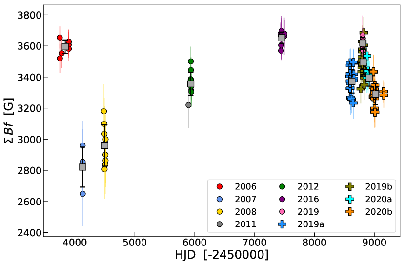
The results for all observations, and averages for each epoch, are presented in Fig. 6, and values for each epoch are provided in Tables 4 and 5. The quantity $\sum Bf$ (sometimes called the magnetic flux, and analogous to a magnetic flux density) ranges between 2.6 kG and 3.7 kG, which is consistent with previous measurements (e.g., Saar, 1994; Kochukhov et al., 2009; Shulyak et al., 2014, 2017, 2019; Cristofari et al., 2023). We observe a long-term increase of the average $\Sigma\,Bf$ from 2.8 kG in 2007 to 3.6 kG in 2016, followed by a weakening towards 3.4 kG with the latest SPIRou observations. Such behaviour correlates with the long-term decrease (in absolute value) of the longitudinal field (Pearson coefficient $R$=0.6, excluding the 2006 data point). Likewise, the average $\Sigma\,Bf$ time series correlates with the average FWHM of Stokes $I$, demonstrating its capability at tracing the evolution of the total, unsigned magnetic field (Donati et al., 2023).

The $\Sigma\,Bf$ values for the ESPaDOnS optical data acquired in 2006 fall out from this trend. This could stem from residuals of the telluric correction blending with the lines used in the modelling and/or instrumental effects such as fringing, for which the results are sensitive to the choice of continuum normalisation. Attempts were made to correct for these potential systematic errors: rejecting observations where the telluric correction left residual features in the used portion of the spectrum, and careful continuum normalisation to remove any weak fringing. However, it is possible these attempts were not fully successful, and thus the departure from the general trend of the 2006 result should be treated with caution.

Figure 6: Long-term evolution of the magnetic flux density measured from Zeeman broadening modelling. The data point format is the same as Fig. 2, and for each epoch we overplotted the mean value and standard deviation as error bar. There is an overall trend that reflects the variations of B_l across both optical and near-infrared data. In addition, for the near-infrared SPIRou time series, we also observe the same oscillating behaviour found for the FWHM of Stokes $I$.

3.4 Magnetic imaging

Figure 7: Full SPIRou and ESPaDOnS 2019 time series of Stokes $V$ profiles of AD Leo normalised by the unpolarised continuum intensity. Two panels are present for 2019a (top left), 2019b (top right), one panel for 2019 in optical (bottom left) and 2020a (bottom middle) and two panels for 2020b (bottom right). In all panels, both the observed profiles (black) and Unno-Rachkovsky models (red) are shown. They are shifted vertically for visualisation purposes, and their associated rotational cycle is reported on the right (see Eq. 1). A remarkable feature is the increased intermittency of the profiles amplitude for the most recent observations, for example at cycle 174.44 and 174.95 of 2020b against cycle 1.40 and 1.88 in 2019a, suggesting an evolution of the magnetic field obliquity.

We applied ZDI to the SPIRou and 2019 ESPaDOnS time series of Stokes $V$ profiles to recover the large-scale magnetic field at the surface of AD Leo. The magnetic geometry is modelled as the sum of a poloidal and a toroidal component, which are both expressed through spherical harmonics decomposition (Donati et al., 2006; Lehmann & Donati, 2022). The algorithm compares observed and synthetic Stokes $V$ profiles iteratively, fitting the spherical harmonics coefficients $\alpha_{\ell,m}$, $\beta_{\ell,m}$, and $\gamma_{\ell,m}$ (with $\ell$ and $m$ the degree and order of the mode, respectively), until they match within a target reduced $\chi^{2}$. Because the inversion problem is ill-posed, a maximum-entropy regularisation scheme is applied to obtain the field map compatible with the data and with the lowest information content (for more details see Skilling & Bryan 1984; Donati & Brown 1997; Folsom et al. 2018).

In practice, we used the zdipy code described in Folsom et al. (2018). In its initial version, the code performed tomographic inversion under weak-field approximation, for which Stokes $V$ is proportional to the first derivative of Stokes $I$ over velocity (Landi Degl’Innocenti & Landolfi, 2004). For the present study, we have implemented the Unno-Rachkovsky’s solutions to polarised radiative transfer equations in a Milne-Eddington atmosphere (Unno, 1956; Rachkovsky, 1967; Landi Degl’Innocenti & Landolfi, 2004) and incorporated the filling factor formalism outlined in Morin et al. (2008b) and Donati et al. (2023). The implementation of Unno-Rachkovsky’s solutions was motivated by the need of a more general model for the observed Stokes V profiles. Near-infrared observations of stars with intense magnetic fields are indeed more susceptible to distortions and broadening due to an enhanced Zeeman effect.

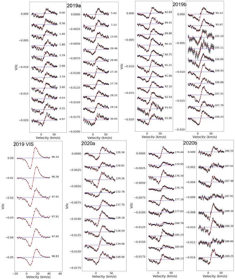
As input parameters for ZDI, we assumed $i=$ 20^∘, $v_{e}\sin(i)=$ 3 km s^-1, P${}_{\mathrm{rot}}=$ 2.23 days, and solid body rotation. We adopted a linear limb darkening coefficient in H band of 0.3 and V band of 0.7 (Claret & Bloemen, 2011). We set the maximum degree of the harmonic expansion $\ell_{\mathrm{max}}=$ 8 (considering the low $v_{e}\sin(i)$) and allowed an entropy weighting scheme proportional to $\ell$ during ZDI inversion, to favour simple geometries as in Lavail et al. (2018). The SPIRou near-infrared time series was split similarly to Sec. 3.1: 2019a (21 observations over 30 cycles), 2019b (21 observations over 26 cycles) 2020a (30 observations over 20 cycles), and 2020b (18 observations over 15 cycles). The Stokes V time series of SPIRou and 2019 ESPaDOnS data are shown in Fig. 7.

Figure 8: Reconstructed ZDI maps in flattened polar view of AD Leo for the SPIRou and 2019 ESPaDOnS time series. The columns correspond to the epochs examined, from the left: 2019a, 2019b, 2019 optical, 2020a, and 2020b. In each column, the radial (top), azimuthal (middle) and meridional (bottom) components of the magnetic field vector are displayed. The radial ticks are located at the rotational phases when the observations were collected, while the concentric circles represent different stellar latitudes: -30 ^∘, +30 ^∘ and +60 ^∘ (dashed lines) and equator (solid line). The colour bar range is set by the maximum (in absolute value) of the magnetic field and illustrates the positive (red) and negative (blue) polarity for each epoch.

Figure 9: Evolution of the magnetic field obliquity with respect to the stellar rotation axis. Values estimated from Eq. 3 (Stibbs, 1950) using optical and near-infrared data are illustrated as circles and pluses, colour-coded by epoch, whereas values from ZDI are shown as diamonds and crosses. The y axis is expressed in degrees of colatitude.

For the 2019a, 2019b, 2020a, and 2020b epochs, we fitted the Stokes $V$ profiles to a $\chi^{2}_{r}$ level of 1.2, 1.0, 1.1, and 1.1 from an initial value of 10.3, 15.8, 14.7, and 8.5, respectively. For the ESPaDOnS 2019 time series, we fitted down to $\chi^{2}_{r}=2.5$ from an initial value of 156.3. We attempted to merge the 2019b and 2020a epochs and reconstruct a single map, since they are separated by the shortest time gap. The quality of the final model is deteriorated ($\chi^{2}_{r}$=1.3) with respect to the two epochs separately, but the corresponding map and magnetic energies are consistently recovered. We therefore kept these two epochs separate.

From Fig. 7, it is evident that the near-infrared Stokes $V$ profiles manifest structures and stochastic variability in both lobes. This is not extended in the continuum, since the residuals with respect to the mean profile are compatible with the noise level, it is not rotationally-modulated, and it is not exhibited by Stokes $N$. The presence of such variability was already suggested by the phase-folded variations in B_l (Fig. 2), as some data points featured a departure from a pure rotational modulation. Likewise, the residuals of the Stokes $I$ profiles show clear variability, but the application of a 2D periodogram does not reveal any significant periodicity. While our ZDI model is capable of describing the general shape of Stokes $V$ profiles, it is limited at reproducing the structures and at capturing all the information present. These considerations are also valid for optical observations in 2019, as the amplitude of Stokes $V$ is not matched exactly by our ZDI model, and overall translate into an underestimate of the field strength. This motivates further the use of the PCA method described by Lehmann & Donati (2022), which is a data-driven approach offering a complementary view on the magnetic field evolution, as outlined in the next section.

We are able to constrain the filling factor $f_{V}$ following a $\chi^{2}$ minimisation prescription similar to (Petit et al., 2002). We found $f_{V}$ values oscillating between 9% in 2019a, 16% in 2019b and back to $\sim$11% in the remaining epochs, compatible with Morin et al. (2008b), and larger by a factor of 1.7 than Lavail et al. (2018). This would indicate a weakening of the local small-scale field since 2016, on top of a decrease in large-scale field intensity as seen in the reconstructions (Fig. 8).

The filling factor $f_{I}$ was inspected by considering a grid of values between 0% and 100%; for each $f_{I}$ value, we synthesised a time series of model Stokes $I$ profiles, computed the corresponding time series of $\chi^{2}_{r}$ with the observations, and phase-folded the $\chi^{2}_{r}$ curve at P_rot. We then assessed at what value of $f_{I}$ the $\chi^{2}_{r}$ curve would start manifesting rotational modulation, because it would indicate that certain model profiles deviate from the observations. We noticed that values above 30% deteriorate the fit of the profile core progressively, yielding variability and rotational modulation of the Stokes $I$ profiles, which is not observed otherwise (see Sec. 3.2). Values of $f_{I}=30\%$ are three times larger than $f_{V}$, in agreement with (Morin et al., 2008b). Since the plausible $f_{I}$ values are consistent with 0%, we adopted $f_{I}=0\%$ in the ZDI modelling.

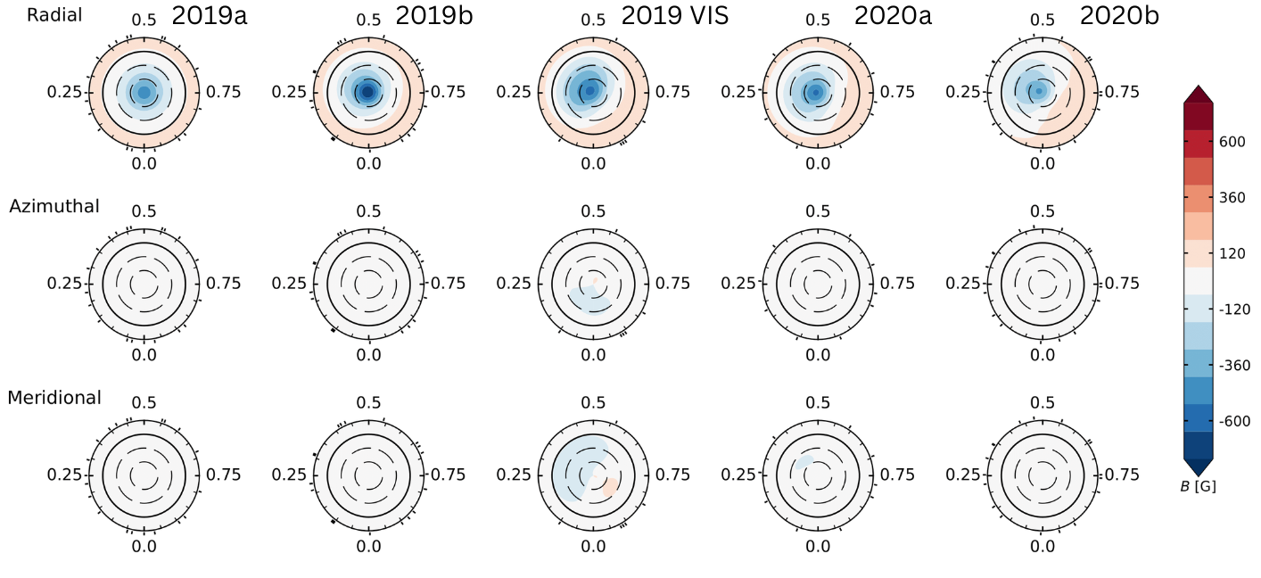
The five maps of surface magnetic flux (one for each SPIRou epoch, and one for the ESPaDOnS 2019 epoch) are shown in Figure 8 and their properties are reported in Table 3. In all cases, the configuration is predominantly poloidal, storing $>$95% of the magnetic energy. The main modes are dipolar and quadrupolar, as they account for 70-90% and 15-20% of the magnetic energy. We report a weakening of the mean field strength ($\langle B\rangle$) of factor of 1.5 and 2.4 relative to the optical maps reconstructed by Morin et al. (2008b) and Lavail et al. (2018), respectively. The most remarkable feature is the reduction of magnetic energy contained in the axisymmetric mode, going from $>$ 99% in 2019a to 60% in 2020b, translating into an increase of the dipole obliquity relative to the rotation axis, from $3^{\circ}$ to $38^{\circ}$.

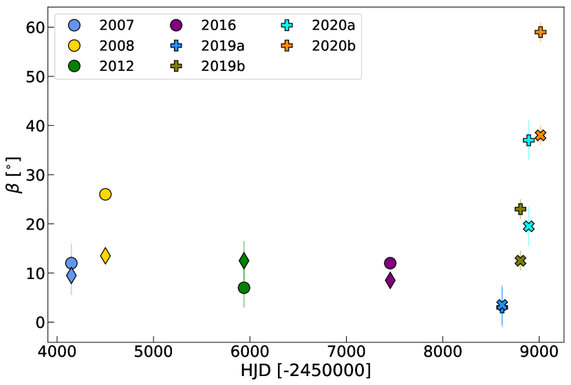
We note that the maximum field strength reconstructed with ZDI is between 1.2 and 2.4 times smaller than obtained via Eq. 3 (Stibbs, 1950). Likewise, the magnetic field obliquity is underestimated, as illustrated in Fig. 9. On one side, this difference stems from the limitation of the Stokes $V$ ZDI model, since it does not encompass the full amplitude of the two lobes for some observations, and on the other side Eq. 3 assumes a purely dipolar field, contrarily to our reconstructions (the dipole accounts for 70-90% of the energy). Nevertheless, both approaches allow us to observe an evident evolution of the obliquity, featuring a rapid increase in the most recent epochs.

Finally, we merged the 2019b, 2020a and 2020b data sets and attempted a joint rotation period and differential rotation search following Petit et al. (2002). The results were inconclusive, likely due to the significant evolution of the surface magnetic field between each epoch.

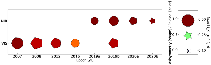
The summary of the magnetic field’s evolution is illustrated in Fig. 10. We performed ZDI reconstructions also for the archival ESPaDOnS and Narval data for consistency, finding reasonably compatible results with previous studies (Morin et al., 2008b; Lavail et al., 2018). We observe a globally simple geometry (i.e. predominantly poloidal and dipolar) over 14 yr, with a decreasing strength. Our latest SPIRou observations revealed a clear evolution of the dipole obliquity in the form of a reduced axisymmetry, suggesting a potential dynamo magnetic cycle. These features are indeed compatible with the variations observed by Sanderson et al. (2003) and Lehmann et al. (2021) for the solar cycle.

Figure 10: Evolution of the magnetic topology of AD Leo over 14 yr. The time series includes optical ESPaDOnS and Narval data between 2007 and 2019, and near-infrared SPIRou data collected between 2019 and 2020. Field strength, level of axisymmetry and dominant field component (poloidal or toroidal) are encoded with the symbol size, shape, and colour, respectively, and were computed using the Unno-Rachkovsky implementation described in this work for consistency. The topology remained predominantly poloidal and dipolar, while the field strength has decreased over time. The most striking change is a decrease in axisymmetry in the most recent epoch.

Table 3: Properties of the magnetic maps for the 2019a, 2019b, 2020a, and 2020b SPIRou epochs and the 2019 ESPaDOnS data set.

	2019a	2019b	2019	2020a	2020b
	NIR	NIR	VIS	NIR	NIR
fV	9%	16%	12%	12%	11%
$\langle B\rangle$ [G]	111.2	132.3	158.0	115.3	93.4
Bmax [G]	481.2	764.0	577.2	555.1	434.3
Bpol [%]	100.0	99.9	95.0	99.3	98.7
Btor [%]	0.0	0.1	5.0	0.7	1.3
Bdip [%]	81.3	71.1	81.7	75.7	70.1
Bquad [%]	14.9	19.0	14.6	17.7	21.2
Boct [%]	2.8	6.2	2.7	4.4	5.9
Baxisym [%]	99.8	94.5	77.0	85.8	58.3
Obliquity [∘]	2.5	12.5	21.5	19.5	38.0

3.5 Diagnosing the large-scale field using PCA

AD Leo is an ideal target for analysing large-scale field evolution with the data-driven PCA method recently presented by Lehmann & Donati (2022), given its magnetic field strength and $v_{e}\sin(i)$. Principal component analysis allows us to uncover details about the stellar large-scale field directly from the LSD Stokes $V$ profiles and to trace its magnetic field evolution across the observation run, without prior assumptions. Here, we analyse only the near-infrared time series, because the number of optical 2019 observations is not sufficient.

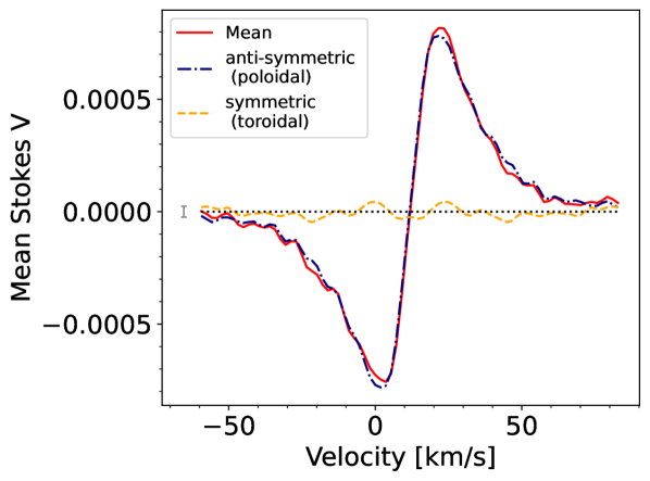
First, we can get insights about the star’s axisymmetric large-scale field by analysing the mean Stokes $V$ profile determined over all Stokes $V$ LSD profiles (see Lehmann & Donati (2022) for further details). Fig. 11 displays the mean profile and the decomposition into its antisymmetric and symmetric parts, denoting the poloidal and toroidal axisymmetric components, respectively. We clearly see that the mean profile is antisymmetric, which indicates a poloidal-dominated axisymmetric large-scale field. The amplitude of the symmetric part is comparable to the noise, and likely due to an artefact of uneven phase coverage rather than a true toroidal field signal (Lehmann & Donati, 2022). Compared to the mean-subtracted Stokes $V$ profiles, the amplitude of the mean profile is generally strong, marking a dominant axisymmetric field. However, we observe an increase in the amplitude of the mean-subtracted Stokes $V$ in the last two epochs 2020a and 2020b, which provides a first hint towards a less axisymmetric configuration.

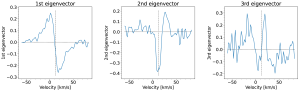
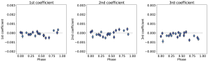
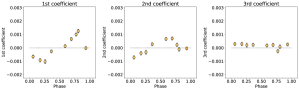
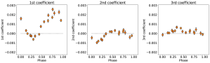
Second, the application of PCA to the mean-subtracted Stokes $V$ profiles yields insights on the non-axisymmetric field, (Lehmann & Donati, 2022). For the mean-subtracted Stokes $V$ profiles, we applied the mean profile computed across all epochs, which allows a direct reflection of the epoch-to-epoch variations in PCA coefficients (e.g. in amplitude and mean value). If the mean Stokes $V$ profile were computed per epoch, we would miss such information, that is to say the mean value of the coefficients would be centred for each epoch, and the amplitudes could no longer be compared to each other. Fig. 12 presents the first three eigenvectors and their corresponding coefficients for the mean-subtracted Stokes $V$ profiles separated by epoch and colour-coded by rotation cycle. The first eigenvector displays an antisymmetric shape proportional to the first derivative of the Stokes $I$ profile and, together with the associated coefficient, scales mainly with the longitudinal magnetic field (Landi Degl’Innocenti & Landolfi, 2004). The second eigenvector shows a more symmetric shape, more closely related to the second derivative of the Stokes $I$ profile, and describes the temporal evolution of the Stokes $V$ profiles between the maxima of the longitudinal field. According to Lehmann & Donati (2022), a strongly antisymmetric eigenvector traces the radial component and a symmetric eigenvector the azimuthal component for a dipole dominated field that is strongly poloidal, which is the case for AD Leo. The third eigenvector features a signal as well (antisymmetric, and related to the third derivative of the Stokes $I$ profile), which is detectable due to the high S/N of the data set, while the further eigenvectors are dominated by noise. Seeing three eigenvectors indicates that even if the axisymmetric field is likely to be dominant, we are able to detect and to analyse the non-axisymmetric field in great detail.

The coefficients of the eigenvectors suggest an evolving large-scale field as their trend changes for every epoch, see Fig. 12 2nd-5th row. In 2019a, the coefficients related to the first eigenvector show only a flat distribution around zero, implying a predominantly axisymmetric field. For the following epochs, 2019b, 2020a and 2020b, we see sine-like trends of the first two coefficients with rotational phase. The amplitude increases from epoch to epoch, indicating a growing obliquity of the dipole-dominated large-scale field. For the 2020b epoch, the obliquity becomes so large that the coefficients of the third eigenvector start to show a sine-like trend as well, which translates into a significant non-axisymmetric field.

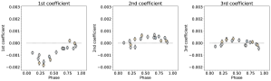
Furthermore, the extremes of the coefficients associated to the antisymmetric and symmetric profile (first and second eigenvector) for the same epoch feature an apparent phase shift of $\approx 0.25$, which demonstrates that the dipolar component is poloidal dominated with little to no toroidal contribution (Lehmann & Donati, 2022). The extremes of the coefficients related to the antisymmetric eigenvector locate the pointing phase of the dipole (Lehmann & Donati, 2022). For the last three epochs, the maximum of this coefficient occurs at a pointing phase of $\approx 0.3$ for the northern pole of the dipole, and the sign of the eigenvector implies a negative polarity. The extremes of the coefficients occur at the same rotational phase throughout the whole observation run, designating a stable pointing phase of the dipole, in agreement with the $B_{\ell}$ measurements (see middle panel of Fig. 2).

By applying the PCA method on the time series of Stokes $V$ (Lehmann & Donati, 2022), we confirm that AD Leo features a dipolar large-scale field, whose obliquity increased during the latest epochs (2020a and 2020b). As the large-scale field became more non-axisymmetric, the pointing phase of the dipole remained stable.

Figure 11: Decomposition of the Stokes $V$ mean profile of AD Leo SPIRou observations. The mean profile (solid red line) and its antisymmetric (dash dotted blue line) and symmetric (dashed yellow line) parts, related to the poloidal and toroidal components of the axisymmetric large-scale field, are shown.

Figure 12: Principal component analysis applied to the mean-subtracted Stokes $V$ profiles. The first three eigenvectors (top row) and their corresponding coefficients (2nd-4th row) are shown. The vertical line in the eigenvector panels indicates the radial velocity offset for AD Leo, of approximately 12.4 km s^-1, while the horizontal dotted line in all panels represents the null line. The coefficients are displayed by epoch: 2019a (2nd row), 2019b (3rd row), 2020a (4th row) and 2020b (5th row). They are phase folded using Eq. 1 and colour-coded by rotation cycle.

4 Achromaticity of the magnetic field

The impact of stellar magnetic activity on radial velocity measurements features a chromatic dependence stemming from a combination of magnetic field and spot temperature contrast (Reiners et al., 2013; Baroch et al., 2020). Indeed, at near-infrared wavelengths the Zeeman broadening is expected to be stronger, while starspots contribute less owing to a lower contrast with the photosphere. The situation is reversed in the optical domain. For AD Leo, recent work by Carmona et al. (2023) demonstrated the strong chromatic behaviour of radial velocity jitter, the latter being significantly weaker in the near-infrared domain than in optical. The combination of these effects becomes increasingly important with the activity level of the star, since the number of spots would be correspondingly larger (Reinhold et al., 2019), and it could possibly result in distinct contributions to the magnetic field strength, which can then be used to facilitate the modelling of stellar activity.

Fast-rotating stars are expected to feature high active latitudes and large polar spots (e.g., Cang et al., 2020), because the Coriolis force would overcome the buoyancy force, making the flux tubes ascend parallel to the stellar rotation axis (Schuessler & Solanki, 1992; Granzer et al., 2000). There are some cases, however, in which fast rotation does not correlate with the presence of a polar spot (Barnes et al., 2004; Morin et al., 2008a). The fact that AD Leo is a moderate rotator observed nearly pole-on makes it an interesting case to investigate whether longitudinal field measurements are chromatic, reflecting the behaviour of an underlying spot.

Previous studies dedicated to the Sun have shown that the magnetic field strength measured in individual lines varies significantly (Demidov et al., 2008; Demidov & Balthasar, 2012), and differences between optical and near-infrared domains have unveiled a dependence of the field strength on atmospheric height: the field increases while going towards deeper internal layers (Zayer et al., 1989; Solanki, 1993). For other stars, Valenti et al. (1995) reported a chromatic difference in magnetic field strength for the moderatively active K dwarf $\varepsilon$ Eri, but attributed its origin to incomplete modelling of the spectral lines used for the Zeeman broadening analysis. No wavelength dependence of the field strength was reported more recently, neither for $\varepsilon$ Eri (Petit et al., 2021) nor for T Tauri stars (Finociety et al., 2021). The same conclusion was reached by Bellotti et al. (2022) when computing longitudinal field values for the active M dwarf EV Lac using blue ($<550$ nm) and red ($>550$ nm) lines of an optical line list.

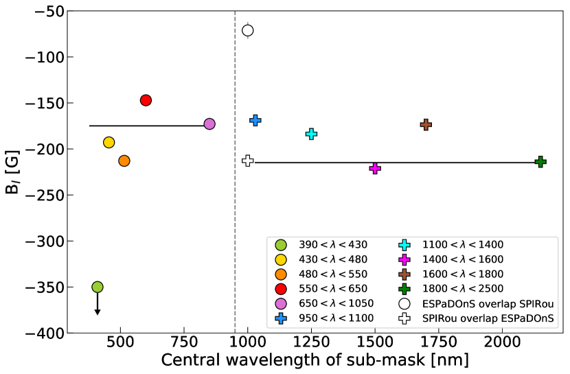
To investigate the longitudinal field chromaticity, we analyse the contemporaneous observations taken with SPIRou and ESPaDOnS in November 2019. We limit the LSD computation within successive wavelength bins of the line mask, and evaluate the longitudinal field for each case. Including both optical and near-infrared domains, we considered 11 subsets of lines in the following ranges: [350,390], [390,430], [430,480], [480,550], [550,650], [650,1100], [950,1100], [1100,1400], [1400,1600], [1600,1800], [1800,2500] nm. The [650,1100] and [950, 1100] nm ranges represent the red end of ESPaDOnS spectra and the blue end of SPIRou spectra, respectively. We adopt more wavelength regions than those presented in Bellotti et al. (2022), allowing a finer search of chromatic trends. The number of lines used varies between 100 and 1000 in the optical, and between 120 and 300 in the near-infrared (see Fig. 16). In addition, we compute LSD using a 50-lines mask in the overlapping wavelength region of ESPaDOnS and SPIRou spectra ([950,1050] nm).

Stokes $I$ and $V$ profiles were computed for the simultaneous SPIRou and ESPaDOnS epochs, namely 2019b and 2019, respectively. To increase the S/N and allow a more precise estimate of B_l, the profiles obtained with a specific line list subset and belonging to the same epoch were co-added. This is reasonable considering the marginal amplitude variation over the epochs examined and the unchanged polarity of Stokes $V$. The longitudinal field was then computed with Eq. 2 using the specific normalisation wavelength and Landé factor of each line subset, and adapting the velocity integration range according to the width of the co-added Stokes $V$ profile.

From Fig. 13, we observe no clear chromaticity of B_l. The distribution of field strength is flat around $-$200 G with a total scatter of 20 G. Such dispersion is mainly due to LSD computations with a low number of lines, implying Stokes shapes more sensitive to variations in individual lines, blends and residuals of telluric correction. For the same reason, some profiles appear deformed and lead to evident outliers (see Fig.16). For instance, the B_l value obtained from ESPaDOnS data in the spectral region overlapping with SPIRou is 100 G weaker (in absolute value) than the B_l value obtained from SPIRou data in the same wavelength region. This could be due to the low S/N at the very red edge of ESPaDOnS.

The case of [390,430] nm leads to a field value of $-$750 G, despite the Stokes profiles do not show a particular deformation. We attribute this behaviour to an imprecise continuum normalisation of the spectra, likely due to a challenging identification of the continuum level in the blue part of the spectrum, where M dwarfs feature forests of spectral lines. The effect is a smaller depth (and equivalent width) of the Stokes $I$ profile relative to the other cases, which artificially increases the value of the field (in absolute value). Overall, although the [350,390] and [390,430] nm bins contain more than half of the lines in the optical mask, their weight in the LSD computation is small (Kochukhov et al., 2010) making their effect in the computation of B_l with the full mask negligible.

Figure 13: Test on B_l measurements chromaticity. Shown are B_l measurements obtained with line mask subsets based on wavelength of the optical (circles) and near-infrared (pluses) domain. The horizontal black lines indicate the values of B_l computed with the full masks and the vertical dashed line separates arbitrarily optical from near-infrared measurements. The error bars are smaller than the symbol size. For visualisation purposes, the [350, 390] nm wavelength bin is not shown since it leads to an outlier data point at around $-$1 kG, and the [390, 430] nm bin yields a value at $-$750 G so it is indicated with a downward arrow. Overall, no chromatic trend emerges from the data.

Figure 14: Dependence of the magnetic field strength on limb darkening. A monotonic decreasing (in absolute value) trend is observed from large (optical) to small (near-infrared) coefficient values. This effect is small, and negligible compared to noise in real observations.

We repeated the same exercise for the other SPIRou epochs and found a similar behaviour, the only difference being 2020b data points shifting upwards because of the field global weakening. A possible implication of the lack of a chromatic trend may be the absence of a polar spot for AD Leo. This would be justified considering that other faster-rotating M dwarfs like V374 Peg (Morin et al., 2008a) and HK Aqr (Barnes et al., 2004) do not show polar spots.

A potential source of chromaticity for B_l values may come from limb darkening. This radial gradient in stellar brightness over the visible disk can be expressed as a linear function of the angle between the line of sight and the normal to a surface element ($\theta$)

$$\frac{I}{I_{0}}=1-\varepsilon(1-\cos\theta),$$ (4)

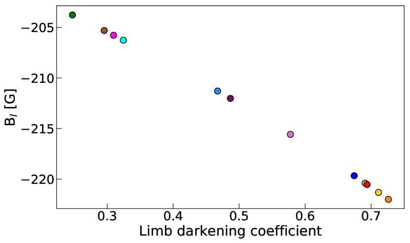
where $I_{0}$ is the brightness at disk centre ($\theta=0^{\circ}$) and $\varepsilon$ is the limb darkening coefficient. Claret & Bloemen (2011) show that $\varepsilon$ decreases with wavelength, being 0.7 in V band and 0.3 in H band. The linear limb darkening law in Eq.4 is the one implemented in the ZDI reconstruction (Folsom et al., 2018).

Owing to the stronger limb darkening in optical than in near-infrared, there is the possibility of additional polarity cancellation in the latter domain, which would lead to weaker field measurements. For the specific case of AD Leo, the low stellar inclination makes the equator appear at the limb and near-infrared observations would be more sensitive to this region. In particular, the sign of large-scale dipolar magnetic field lines exiting the pole would cancel out more with those at equator, compared to optical observations.

To verify this, we 1) linearly interpolated the limb darkening coefficients in Claret & Bloemen (2011) at the wavelengths examined for the thermal contrast test (see Fig. 13), 2) synthesised Stokes profiles for the same coefficients assuming an axisymmetric dipole of 1 kG seen pole-on (akin to AD Leo in 2019a) and infinite S/N, and 3) computed the associated field values with Eq. 2. The results are illustrated in Fig. 14. We observe a small (7%) weakening of the field from optical to near-infrared, which is overwhelmed by noise in real observations.

5 Discussion and conclusions

In this paper, we presented the results of an extended spectropolarimetric monitoring of the active M dwarf AD Leo, using near-infrared observations collected with SPIRou between 2019 and 2020 as part of the SLS survey. They add to the previous optical data obtained with ESPaDOnS and Narval between 2006 and 2019, making the entire time series encompass approximately 14 yr. To carry out our magnetic analysis, we computed the longitudinal magnetic field, tracked the variations of the Stokes $I$ FWHM, modelled Zeeman broadening on individual selected lines, reconstructed the large-scale field topology via ZDI, and assessed axisymmetry variations by means of a novel PCA method.

Initially, Morin et al. (2008b) reported an axisymmetric, dipole-dominated structure that was stable over one year; later, Lavail et al. (2018) pointed out a large-scale weakening and small-scale enhancement of the field but no variation in the geometry. We found strong evidence of a large-scale field evolution, that is summarised as follows:

1. The longitudinal magnetic field has weakened between 2006 and 2020, from $-300$ to $-50$ G, with a rapid decrease of 100 G in the 2020b. The dipolar longitudinal magnetic field evolved in the same time frame, starting from -850 G in 2006, reaching -560 G in 2016 and restoring back to -900 G in 2020.

2. The FWHM of Stokes $I$ profiles does not show rotational modulation, but a dispersion that may partly be due to short-term variability. The epoch-averaged FWHM manifests a long-term variation both in optical and near-infrared, being wider in 2019b and 2020a, and narrower in 2019a and 2020b. The variations are enhanced when the Stokes profiles are computed with magnetically-sensitive lines, as opposed to the insensitive ones. The near-infrared data in particular feature a trend moderately correlated with B_l (in absolute value).

3. The magnetic flux estimated from the modelling of Zeeman broadening exhibits a global increase over time, which is also correlated to the long-term trend of the longitudinal magnetic field (in absolute value). Moreover the epoch-averaged magnetic flux obtained for the near-infrared SPIRou time series oscillates in a similar manner to the FWHM of Stokes $I$, demonstrating that the latter is capable of tracing secular evolution of the total, unsigned magnetic field.

4. Zeeman-Doppler imaging reconstructions confirmed the same kind of topological evolution, with the axisymmetric level decreasing to $60\%$ and the obliquity between magnetic and rotation axis increasing to $38^{\circ}$. This already found support by the enhanced intermittency of the amplitude of Stokes $V$ profiles in late 2020.

5. The PCA method confirmed the predominantly poloidal and dipolar geometry of the large-scale field, as well as a lower axisymmetry in 2020a and 2020b. In addition, the pointing phase of the dipole remained stable during the evolution.

6. Measurements of the magnetic field strength are overall achromatic, since they manifest only a marginal wavelength dependence due to limb darkening.

Our results altogether suggest that AD Leo may be entering a polarity reversal phase of a long-term magnetic cycle, analogous to the solar one. The combination of chromospheric activity studies and spectropolarimetric campaigns show that some Sun-like stars may manifest magnetic cycles and polarity reversals in phase with chromospheric cycles (Boro Saikia et al., 2016; Jeffers et al., 2017), while others have a more complex behaviour where very regular chromospheric oscillations have no straightforward polarimetric counterpart (Boro Saikia et al., 2022).

Predicting when the polarity reversal may occur for AD Leo is not a trivial task, as the B_l data set does not feature a clear minimum or maximum. Recently, Fuhrmeister et al. (2023) did not report any evident trends from a long-term campaign of chromospheric indexes, whereas previous studies based on photometric observations reported either two co-existing timescales for cycles, namely 7 yr and 2 yr (Buccino et al., 2014), or an individual one of about 11 yr (Tuomi et al., 2018). However, these time scales are not compatible with the variations in B_l observed over 14 yr. The axisymmetric level of the large-scale topology is a more suitable proxy to track the cycle (Lehmann et al., 2021), but we recorded its change only in the most recent observations.

A comparison between the magnetic field evolution described here and that of the radial velocity jitter obtained in Carmona et al. (2023) leads to a puzzling situation. Carmona et al. (2023) show that radial velocity variations in optical are essentially due to the presence of a spot and that this signal has changed only slightly (in phase and amplitude, the latter varies from 25.6$\pm$0.3 m s^-1 to 23.6$\pm$0.5 m s^-1) between 2005 and 2021. Such radial velocity signal is not detected in infrared with SPIRou, corroborating its strong chromaticity and therefore its origin due to stellar activity Carmona et al. (2023). The fact that the dipolar field evolution is disjointed from a surface brightness evolution is not a surprise: Morin et al. (2008a) show that the mainly-dipolar topology of V374 Peg did not correlate with the complex brightness map reconstructed via Doppler imaging.

These considerations motivate long-term spectropolarimetric and velocimetric campaigns of active M dwarfs. For AD Leo in particular, additional monitoring is required to observe the polarity reversal and the cycle’s extremes, to constrain a precise time scale. An extended temporal baseline could also give more insight on the link between topological variations and high-energy flaring events (e.g., Stelzer et al., 2022). At the same time, we could shed more light on the relation between the evolution of the large-scale magnetic field topology and the stability of the radial velocity jitter.

An additional detail we could infer about AD Leo’s magnetic field is the helicity, which quantifies the linkage between poloidal and toroidal field lines and thus describes the complexity of the magnetic topology (Lund et al., 2020, 2021). For the Sun, Pipin et al. (2019) reported a temporal variation of the value correlated to the magnetic cycle. Indeed, helicity maxima and minima occur when the axis of symmetry of the poloidal and toroidal field components are aligned and orthogonal, respectively.

For AD Leo, the fraction of toroidal energy is only a negligible fraction of the total one, hence we should exert caution when deriving quantities from it. Over time, we observe that the poloidal axisymmetric ($m=0$) mode maintains $>$80% of the magnetic energy and features a drop to 45% in 2020b, while the energy in the toroidal axisymmetric mode decreases from 30% to 6%. As a result, the two components maintained an overall misaligned configuration, but in the most recent epoch, the poloidal component became more aligned with the toroidal one due to the axisymmetry decrease. Following the practical visualisation of Lund et al. (2021), this evolution would correspond to an increase in field helicity.

The existence of a magnetic cycle for AD Leo is in agreement with the observational evidence of such phenomena for M dwarfs from radial velocity exoplanet searches (Gomes da Silva et al., 2012; Lopez-Santiago et al., 2020). In general, studies have shown that magnetic cycles introduce long-term signals in radial velocity data sets that can dominate over planetary signatures (Meunier et al., 2010; Meunier & Lagrange, 2019), as they modulate the appearance and number of heterogeneities on the stellar surface. It is therefore necessary to have an accurate constraint on the temporal variations of the cycle, in order to remove its contamination and allow a more reliable planetary detection and characterisation (Lovis et al., 2011; Costes et al., 2021; Sairam & Triaud, 2022).

Furthermore, activity cycles modulate the stellar radiation output and winds in which close-in planets are immersed (Yeo et al., 2014; Hazra et al., 2020). This leads to a temporal variation in the planetary atmospheric stripping with consequent alteration of the chemical properties and habitability (Lanza, 2013; McCann et al., 2019; Louca et al., 2023; Konings et al., 2022). Details on the occurrence of the cycle extremes can thus inform the most suitable interpretation framework and observing plans for missions dedicated to transmission spectroscopy like $Ariel$ (Tinetti et al., 2021). At the same time, periodic variations in the large-scale field geometry need to be considered for an accurate and updated modelling of the low-frequency radio emission discovered for M dwarfs (Callingham et al., 2021), which has been recently proposed to potentially reveal the presence of close-in magnetic planets (Vedantham et al., 2020; Kavanagh et al., 2021, 2022).

Finally, AD Leo may not be an isolated case. To verify this, it is essential to explore the possibility for such cycles over a wider area of the stellar parameter space, namely mass and rotation period.

Appendix A FWHM of Stokes I

In this appendix, the Stokes $I$ profiles computed using different line selections are shown. We compare the width of the profiles obtained with the full atomic mask, high-Landé factor (g${}_{\mathrm{eff}}>1.2$) lines and low-Landé factor (g${}_{\mathrm{eff}}<1.2$) lines.

Figure 15: Median Stokes $I$ profiles computed for the four near-infrared epochs: 2019a, 2019b, 2020a, and 2020b. The profiles are obtained using the full mask (top) magnetically sensitive (middle) and insensitive (bottom) line lists in LSD. Following the linear dependence of the Zeeman effect on the Landé factor, high-g_eff lines are broader than low-g_eff lines on average. The width of the profiles changes over time in the high-g_eff case, while it remains reasonably constant in the low-g_eff case.

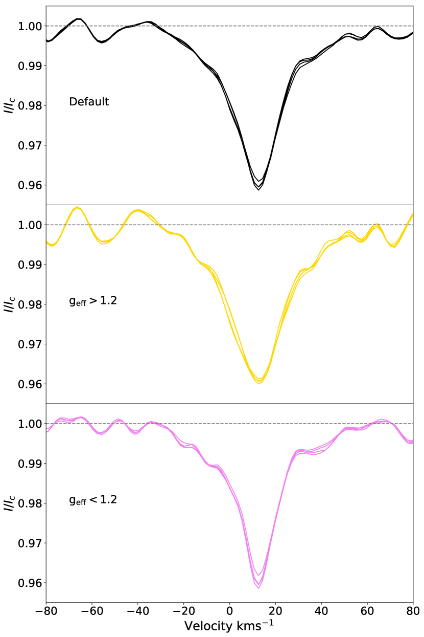
Appendix B Chromatic Stokes profiles

The various Stokes profiles computed with different wavelength-based line lists for LSD are reported. The wavelength intervals of the line subsets are: [350,390], [390,430], [430,480], [480,550], [550,650], [650,1100], [950,1100], [1100,1400], [1400,1600], [1600,1800], [1800,2500] nm.

Figure 16: Series of Stokes profiles computed with subsets of the line list used for LSD, as described in Sec.4. Every panel displays Stokes $I$ (top), $V$ (middle) and $N$ (bottom) for each line subset and vertical dashed lines indicate the adjusted velocity range over which B_l was estimated. The optical profiles are obtained by stacking the ESPaDOnS observations from 2019, whereas the near-infrared ones from SPIRou 2019b time series, for each panel. The number of lines used in the LSD computation as well as the mean wavelength are displayed.

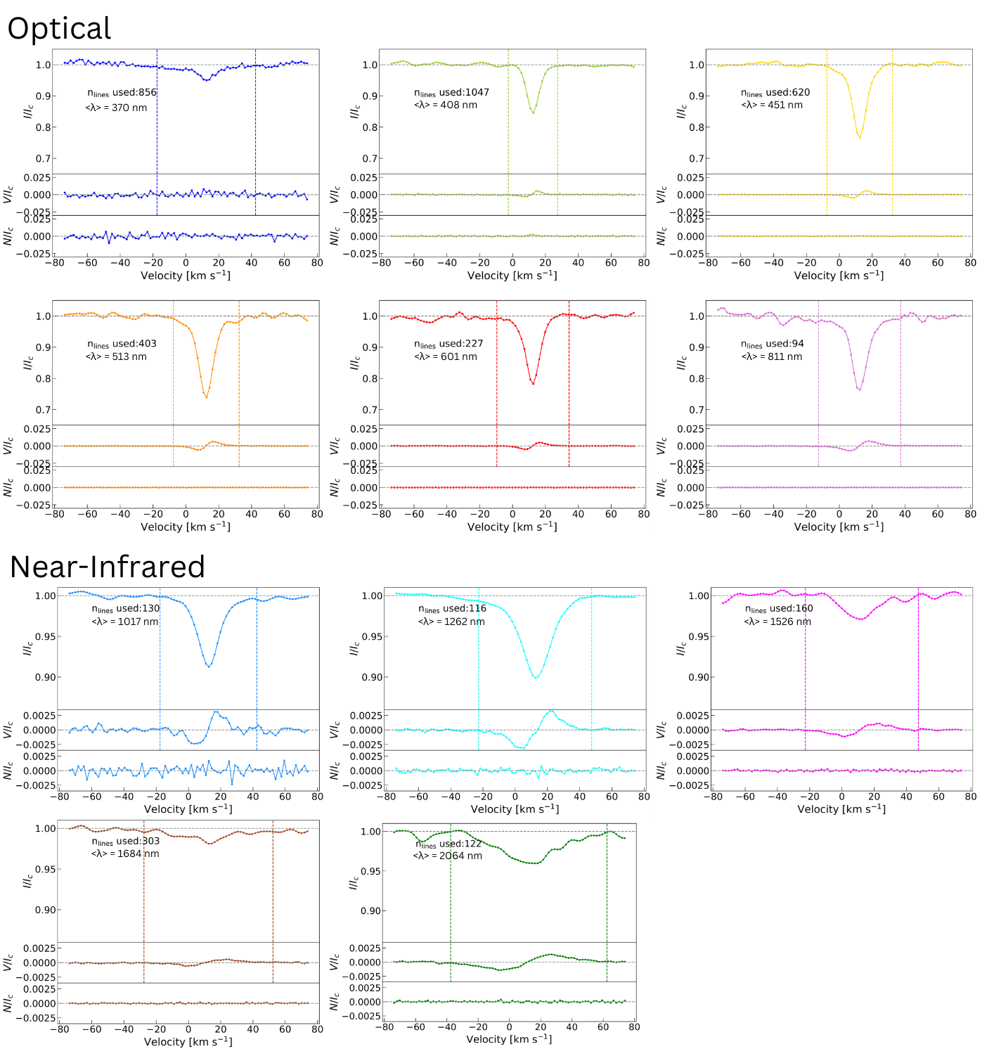
Appendix C Zeeman broadening examples

Example plots of the posterior distributions from the Zeeman broadening MCMC analysis are shown in Fig. 17 for a ESPaDOnS observation and in Fig. 18 for a SPIRou observation. Summaries of the results of the MCMC analysis for each epoch are provided in Tables 4 and 5.

Figure 17: Posterior distribution for parameters from the Zeeman broadening analysis of the ESPaDOnS observation on 24 Febuary 2016. The filling factor for a given magnetic field strength is $f$, and abundances are in $\log n_{X}/n_{\rm H}$ units.

Figure 18: Posterior distribution for parameters from the Zeeman broadening analysis of the SPIRou observation on 3 November 2020.

Table 4: Parameters from the Zeeman broadening analysis, averaged for each epoch, for ESPaDOnS and Narval optical observations. Uncertainties are the standard deviations for each epoch.

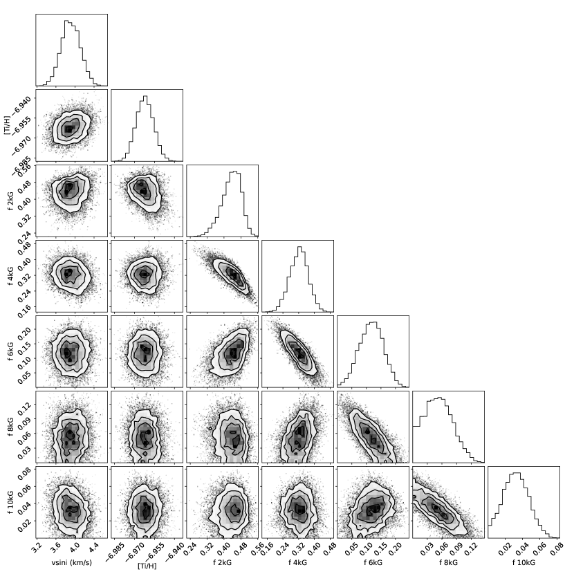
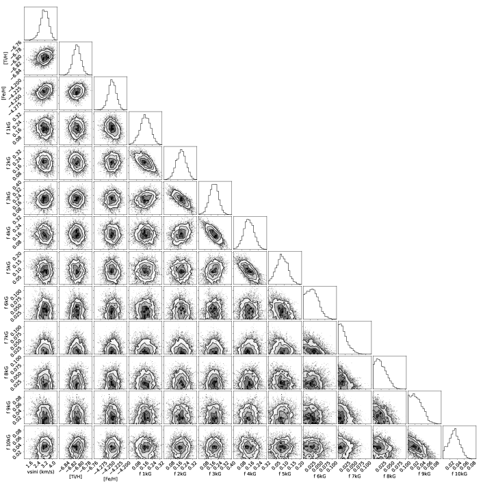
epoch	2006	2007	2008	2011	2012	2016	2019
$v_{e}\sin(i)$ [km s-1]	4.27$\pm$0.38	4.25$\pm$0.17	4.16$\pm$0.29	3.46$\pm$0.50	2.65$\pm$0.48	3.57$\pm$0.21	3.39$\pm$0.45
$[$Ti/H$]$	$-$6.97$\pm$0.01	$-$6.90$\pm$0.01	$-$6.93$\pm$0.02	$-$6.99$\pm$0.01	$-$7.00$\pm$0.01	$-$6.96$\pm$0.01	$-$6.95$\pm$0.01
$f_{0\rm kG}$	0.06$\pm$0.02	0.24$\pm$0.06	0.18$\pm$0.06	0.05$\pm$0.06	0.02$\pm$0.01	0.05$\pm$0.02	0.06$\pm$0.01
$f_{2\rm kG}$	0.46$\pm$0.01	0.32$\pm$0.07	0.39$\pm$0.07	0.60$\pm$0.06	0.52$\pm$0.02	0.44$\pm$0.01	0.41$\pm$0.01
$f_{4\rm kG}$	0.33$\pm$0.02	0.31$\pm$0.02	0.28$\pm$0.04	0.19$\pm$0.07	0.29$\pm$0.01	0.33$\pm$0.01	0.36$\pm$0.01
$f_{6\rm kG}$	0.09$\pm$0.01	0.06$\pm$0.01	0.08$\pm$0.01	0.11$\pm$0.05	0.09$\pm$0.01	0.11$\pm$0.01	0.09$\pm$0.01
$f_{8\rm kG}$	0.05$\pm$0.01	0.03$\pm$0.01	0.04$\pm$0.01	0.04$\pm$0.03	0.05$\pm$0.01	0.05$\pm$0.01	0.05$\pm$0.01
$f_{10\rm kG}$	0.04$\pm$0.01	0.02$\pm$0.01	0.02$\pm$0.01	0.03$\pm$0.03	0.02$\pm$0.01	0.04$\pm$0.01	0.04$\pm$0.01
$\sum Bf$ [kG]	3.59$\pm$0.04	2.82$\pm$0.13	2.97$\pm$0.13	3.22$\pm$0.15	3.37$\pm$0.06	3.65$\pm$0.04	3.62$\pm$0.03

Table 5: Parameters from the Zeeman broadening analysis, averaged for each epoch, for SPIRou observations. Uncertainties are the standard deviations for each epoch.

epoch	2019a	2019b	2020a	2020b
$v_{\mathrm{eq}}\sin(i)$ [km s-1]	3.42$\pm$0.23	3.34$\pm$0.18	3.48$\pm$0.17	3.48$\pm$0.21
$[$Ti/H$]$	$-$6.78$\pm$0.02	$-$6.78$\pm$0.02	$-$6.79$\pm$0.02	$-$6.78$\pm$0.01
$[$Fe/H$]$	$-$4.20$\pm$0.01	$-$4.22$\pm$0.01	$-$4.20$\pm$0.03	$-$4.21$\pm$0.02
$f_{0\rm kG}$	0.06$\pm$0.02	0.05$\pm$0.02	0.05$\pm$0.02	0.06$\pm$0.01
$f_{1\rm kG}$	0.15$\pm$0.02	0.12$\pm$0.03	0.15$\pm$0.02	0.17$\pm$0.02
$f_{2\rm kG}$	0.20$\pm$0.04	0.23$\pm$0.05	0.19$\pm$0.04	0.19$\pm$0.04
$f_{3\rm kG}$	0.24$\pm$0.04	0.19$\pm$0.05	0.23$\pm$0.05	0.24$\pm$0.04
$f_{4\rm kG}$	0.12$\pm$0.04	0.16$\pm$0.04	0.14$\pm$0.03	0.13$\pm$0.03
$f_{5\rm kG}$	0.06$\pm$0.02	0.08$\pm$0.02	0.06$\pm$0.02	0.06$\pm$0.01
$f_{6\rm kG}$	0.05$\pm$0.01	0.05$\pm$0.02	0.05$\pm$0.01	0.04$\pm$0.01
$f_{7\rm kG}$	0.03$\pm$0.01	0.02$\pm$0.01	0.03$\pm$0.01	0.03$\pm$0.01
$f_{8\rm kG}$	0.02$\pm$0.01	0.02$\pm$0.01	0.02$\pm$0.01	0.02$\pm$0.01
$f_{9\rm kG}$	0.03$\pm$0.01	0.03$\pm$0.01	0.03$\pm$0.01	0.03$\pm$0.01
$f_{10\rm kG}$	0.03$\pm$0.01	0.03$\pm$0.01	0.04$\pm$0.01	0.03$\pm$0.01
$\sum Bf$ [kG]	3.40$\pm$0.09	3.49$\pm$0.09	3.44$\pm$0.04	3.29$\pm$0.07

Appendix D Observing log

This appendix contains the journal of observations of AD Leo, for both optical and near-infrared observations. It also includes all measurements of longitduinal magnetic field and $\Sigma Bf$.

Table 6: List of AD Leo observations collected with SPIRou. The columns are: (1 and 2) date and universal time of the observations, (3) rotational cycle of the observations found using Eq. 1, (4) exposure time of a polarimetric sequence, (5) signal-to-noise ratio at 1650 nm per spectral element, (6) RMS noise level of Stokes $V$ signal in units of unpolarised continuum.

Date	UT	$n_{\mathrm{cyc}}$	$t_{exp}$	S/N	$\sigma_{\mathrm{LSD}}$
	[hh:mm:ss]		[s]		[$10^{-4}I_{c}$]
2019
April 15	06:11:02.35	0.00	4x61	151	1.9
April 16	12:03:07.61	0.56	4x61	130	1.8
April 18	09:00:59.77	1.40	4x61	138	1.9
April 19	10:36:14.55	1.88	4x61	143	1.8
April 20	08:56:19.44	2.29	4x61	143	1.8
April 21	05:42:43.43	2.68	4x61	165	1.5
April 22	08:58:10.67	3.19	4x61	147	1.9
April 23	07:01:28.73	3.60	4x61	154	1.9
April 24	06:04:06.74	4.03	4x61	147	1.9
April 25	09:41:45.90	4.55	4x61	152	1.9
April 26	08:13:21.75	4.97	4x61	162	1.9
April 27	08:17:48.22	5.42	4x61	139	2.1
May 01	08:59:11.25	7.23	4x61	153	1.8
May 15	06:11:38.01	13.45	4x61	165	1.6
June 13	06:30.59.49	26.46	4x61	186	2.1
June 14	05:44:29.79	26.89	4x61	193	2.0
June 15	06:04:31.16	27.35	4x61	192	2.1
June 16	05:44:52.21	27.79	4x61	173	1.8
June 17	06:08:46.48	28.25	4x61	150	1.8
June 19	05:47:00.42	29.14	4x61	175	1.5
June 21	06:18:29.14	30.05	4x61	169	1.7
October 16	15:31:29.14	82.69	4x61	180	1.4
October 31	15:32:56.51	89.41	4x61	169	1.6
November 01	15:22:10.08	89.86	4x61	159	1.5
November 02	15:36:52.90	90.31	4x61	170	1.4
November 03	14:53:22.07	90.75	4x61	151	1.5
November 04	15:43:18.06	91.21	4x61	137	1.9
November 05	15:33:34.93	91.66	4x61	164	1.3
November 06	15:37:27.47	92.10	4x61	190	1.5
November 07	15:01:11.73	92.54	4x61	165	1.5
November 09	14:03:02.38	93.42	4x61	116	1.6
November 10	15:51:32.68	93.90	4x61	151	1.5
November 13	14:47:09.89	95.22	4x61	201	1.8
November 14	14:13:58.20	95.66	4x61	197	1.4
December 05	15:12:55.68	105.10	4x61	116	1.4
December 05	15:35:03.10	105.10	4x61	68	1.5
December 07	15:08:39.83	105.99	4x61	133	2.2
December 08	14:29:19.93	106.43	4x61	181	1.8
December 09	14:21:48.74	106.88	4x61	193	1.5
December 10	13:15:39.48	107.31	4x61	194	1.5
December 11	14:58:07.44	107.79	4x61	189	3.0
December 12	14:33:27.45	108.23	4x61	190	3.6
2020
January 26	12:11:48.90	128.36	4x61	218	2.0
January 27	12:07:16.45	128.81	4x61	166	1.5
January 28	12:06:25.46	129.26	4x61	193	1.5
February 05	08:18:51.61	132.78	4x61	174	1.4
February 16	07:39:02.87	137.70	4x61	193	1.8
February 17	09:20:45.46	138.18	4x61	171	1.9
February 18	07:39:13.56	138.59	4x61	191	1.2
February 19	08:37:09.84	139.06	4x61	210	1.5
March 12	09:16:56.32	148.94	4x61	217	2.0
May 08	05:59:01.58	174.43	4x61	194	1.4
May 09	09:42:30.22	174.95	4x61	206	1.5
May 12	09:39:45.19	176.30	4x61	177	1.4
May 13	09:43:17.10	176.75	4x61	204	1.4
May 14	07:46:35.66	177.16	4x61	208	1.5
May 15	09:50:31.27	177.65	4x61	164	1.6
May 31	06:22:44.29	184.76	4x61	215	1.2
June 01	07:29:57.32	185.23	4x61	189	1.3
June 02	06:23:31.70	185.65	4x61	202	1.4
June 03	07:38:43.10	186.13	4x61	196	1.3
June 04	06:32:43.13	186.55	4x61	197	1.3
June 05	06:42:42.88	187.01	4x61	139	1.8
June 06	07:53:54.53	187.48	4x61	167	1.2
June 07	06:58:07.88	187.91	4x61	154	1.6
June 08	06:03:47.85	188.34	4x61	135	1.3
June 08	06:10:09.48	188.34	4x61	143	1.4
June 09	06:31:50.17	188.79	4x61	120	1.3
June 10	06:57:13.44	189.25	4x61	200	1.8
October 31	15:06:44.49	253.75	4x61	205	1.5
November 03	15:29:52.78	255.11	4x61	220	1.5

Table 6: continued.

Table 7: List of AD Leo observations collected with ESPaDOnS in 2019. The columns are: (1 and 2) date and universal time of the observations, (3) rotational cycle of the observations found using Eq. 1, (4) exposure time of a polarimetric sequence, (5) signal-to-noise ratio at 650 nm per spectral element, (6) RMS noise level of Stokes $V$ signal in units of unpolarised continuum.

Date	UT	$n_{\mathrm{cyc}}$	$t_{exp}$	S/N	$\sigma_{\mathrm{LSD}}$
	[hh:mm:ss]		[s]		[$10^{-4}I_{c}$]
November 15	13:24:01.40	96.32	4x300	234	1.7
November 16	14:20:01.30	96.79	4x300	230	1.9
November 19	14:08:04.00	98.13	4x300	151	3.6
November 19	14:33:03.00	98.14	4x300	159	3.2
November 19	14:56:04.00	98.15	4x300	180	2.8
November 21	15:43:01.00	99.06	4x300	265	1.8

Table 8: List of optical and near-infrared measurements of longitudinal magnetic field and magnetic flux. The columns are: (1) Heliocentric Julian date of the observation, (2) B_l with formal error bar (see Eq. 2), and (3) magnetic flux from Zeeman broadening modelling, when a reliable measurement was possible, and (4) the instrument used.

HJD	Bl	$Bf$	Instrument
$[-2450000]$	[G]	[kG]
3747.0876	$-$269.4 $\pm$ 26.4	$3.65^{+0.07}_{-0.08}$	ESPaDOnS
3748.8868	$-$272.4 $\pm$ 15.1	$3.52^{+0.09}_{-0.10}$	ESPaDOnS
3780.0705	$-$280.7 $\pm$ 13.1	$3.55^{+0.10}_{-0.10}$	ESPaDOnS
3895.8047	$-$291.2 $\pm$ 10.7	$3.62^{+0.08}_{-0.09}$	ESPaDOnS
3896.8124	$-$260.1 $\pm$ 7.6	$3.61^{+0.08}_{-0.09}$	ESPaDOnS
3897.8005	$-$266.7 $\pm$ 7.4	$3.63^{+0.08}_{-0.09}$	ESPaDOnS
3898.7785	$-$294.2 $\pm$ 8.1	$3.58^{+0.08}_{-0.10}$	ESPaDOnS
4127.5975	$-$294.6 $\pm$ 16.5	$\ldots$	Narval
4128.6088	$-$248.6 $\pm$ 10.8	$2.95^{+0.16}_{-0.16}$	Narval
4129.5717	$-$296.2 $\pm$ 11.8	$2.85^{+0.21}_{-0.22}$	Narval
4130.6084	$-$253.8 $\pm$ 9.4	$2.65^{+0.21}_{-0.20}$	Narval
4133.6312	$-$274.8 $\pm$ 10.4	$\ldots$	Narval
4134.6112	$-$271.7 $\pm$ 11.4	$\ldots$	Narval
4135.6217	$-$231.4 $\pm$ 10.4	$\ldots$	Narval
4136.5925	$-$294.9 $\pm$ 13.0	$\ldots$	Narval
4276.7715	$-$261.0 $\pm$ 8.2	$\ldots$	ESPaDOns
4485.5177	$-$290.1 $\pm$ 13.2	$3.18^{+0.17}_{-0.20}$	Narval
4489.5683	$-$248.6 $\pm$ 10.3	$3.10^{+0.17}_{-0.18}$	Narval
4492.5379	$-$285.3 $\pm$ 10.7	$\ldots$	Narval
4493.5486	$-$204.6 $\pm$ 10.6	$3.03^{+0.18}_{-0.19}$	Narval
4495.5611	$-$227.2 $\pm$ 12.6	$2.81^{+0.19}_{-0.19}$	Narval
4499.5675	$-$256.8 $\pm$ 11.1	$\ldots$	Narval
4501.5473	$-$288.6 $\pm$ 12.1	$\ldots$	Narval
4502.5475	$-$202.8 $\pm$ 9.7	$\ldots$	Narval
4506.5576	$-$218.9 $\pm$ 10.0	$2.84^{+0.19}_{-0.20}$	Narval
4508.5516	$-$265.5 $\pm$ 11.0	$\ldots$	Narval
4509.5564	$-$219.6 $\pm$ 12.2	$2.90^{+0.18}_{-0.20}$	Narval
4510.5523	$-$286.6 $\pm$ 15.3	$\ldots$	Narval
4511.5694	$-$200.2 $\pm$ 10.5	$2.86^{+0.17}_{-0.17}$	Narval
4512.5537	$-$296.7 $\pm$ 10.8	$2.99^{+0.16}_{-0.16}$	Narval
5896.7560	$-$249.3 $\pm$ 11.5	$3.22^{+0.15}_{-0.16}$	Narval
5934.6407	$-$247.0 $\pm$ 9.5	$3.39^{+0.11}_{-0.12}$	Narval
5935.6765	$-$225.9 $\pm$ 9.3	$3.50^{+0.09}_{-0.11}$	Narval
5936.6050	$-$241.7 $\pm$ 10.9	$3.38^{+0.09}_{-0.10}$	Narval
5937.7575	$-$254.6 $\pm$ 11.2	$3.44^{+0.08}_{-0.10}$	Narval
5938.6659	$-$243.9 $\pm$ 8.8	$3.31^{+0.08}_{-0.10}$	Narval
5939.6031	$-$234.2 $\pm$ 10.6	$3.34^{+0.08}_{-0.10}$	Narval
5940.6416	$-$203.8 $\pm$ 9.1	$3.31^{+0.09}_{-0.09}$	Narval
5941.6411	$-$232.7 $\pm$ 9.7	$3.36^{+0.11}_{-0.13}$	Narval
5942.6256	$-$220.5 $\pm$ 10.2	$3.30^{+0.09}_{-0.10}$	Narval
7435.7957	$-$177.0 $\pm$ 5.5	$3.68^{+0.07}_{-0.08}$	ESPaDOnS
7436.8831	$-$165.8 $\pm$ 5.3	$3.67^{+0.08}_{-0.09}$	ESPaDOnS
7441.8954	$-$181.4 $\pm$ 5.3	$3.57^{+0.06}_{-0.07}$	ESPaDOnS
7443.0074	$-$166.1 $\pm$ 5.3	$3.60^{+0.09}_{-0.10}$	ESPaDOnS
7447.9103	$-$160.7 $\pm$ 6.4	$3.65^{+0.14}_{-0.16}$	ESPaDOnS
7449.0011	$-$182.9 $\pm$ 7.7	$3.66^{+0.11}_{-0.13}$	ESPaDOnS
7449.9154	$-$154.6 $\pm$ 6.5	$3.66^{+0.12}_{-0.15}$	ESPaDOnS
7450.8328	$-$190.5 $\pm$ 6.9	$3.70^{+0.09}_{-0.11}$	ESPaDOnS
7495.8253	$-$192.9 $\pm$ 8.8	$3.66^{+0.12}_{-0.15}$	ESPaDOnS
7498.7442	$-$170.6 $\pm$ 5.8	$3.68^{+0.09}_{-0.09}$	ESPaDOnS
8588.7573	$-$194.7$\pm$17.2	$3.40^{+0.08}_{-0.09}$	SPIRou
8590.0016	$-$212.3$\pm$19.9	$\ldots$	SPIRou
8592.9410	$-$206.5$\pm$17.4	$3.33^{+0.09}_{-0.11}$	SPIRou
8593.8715	$-$202.5$\pm$16.5	$3.37^{+0.11}_{-0.11}$	SPIRou
8594.7370	$-$234.3$\pm$16.8	$3.42^{+0.10}_{-0.11}$	SPIRou
8595.8726	$-$211.7$\pm$16.4	$3.47^{+0.10}_{-0.13}$	SPIRou
8596.7915	$-$217.9$\pm$16.0	$3.37^{+0.09}_{-0.09}$	SPIRou
8597.7516	$-$219.1$\pm$18.6	$3.33^{+0.10}_{-0.09}$	SPIRou
8598.9026	$-$240.0$\pm$16.9	$3.49^{+0.09}_{-0.09}$	SPIRou
8599.8411	$-$263.6$\pm$17.6	$3.36^{+0.09}_{-0.10}$	SPIRou
8600.8441	$-$182.9$\pm$16.7	$3.36^{+0.10}_{-0.11}$	SPIRou
8604.8725	$-$190.5$\pm$16.3	$3.27^{+0.11}_{-0.12}$	SPIRou
8618.7549	$-$216.5$\pm$15.1	$3.27^{+0.08}_{-0.09}$	SPIRou
8647.7665	$-$217.0$\pm$12.9	$3.26^{+0.09}_{-0.09}$	SPIRou
8648.7341	$-$221.3$\pm$13.1	$3.38^{+0.09}_{-0.09}$	SPIRou
8649.7480	$-$230.0$\pm$15.3	$3.23^{+0.10}_{-0.10}$	SPIRou
8650.7343	$-$194.7$\pm$13.6	$3.49^{+0.09}_{-0.10}$	SPIRou
8651.7509	$-$209.4$\pm$16.0	$3.49^{+0.08}_{-0.10}$	SPIRou
8653.7357	$-$227.2$\pm$13.6	$3.38^{+0.09}_{-0.09}$	SPIRou
8655.7575	$-$250.3$\pm$20.3	$3.42^{+0.09}_{-0.10}$	SPIRou
8773.1472	$-$223.6$\pm$14.4	$3.39^{+0.10}_{-0.10}$	SPIRou
8788.1497	$-$223.7$\pm$13.4	$3.32^{+0.09}_{-0.10}$	SPIRou
8789.1423	$-$184.8$\pm$13.7	$3.43^{+0.10}_{-0.09}$	SPIRou
8790.1526	$-$245.2$\pm$15.4	$3.50^{+0.09}_{-0.10}$	SPIRou
8791.1225	$-$192.7$\pm$13.8	$3.50^{+0.12}_{-0.12}$	SPIRou
8792.1572	$-$256.3$\pm$16.3	$3.46^{+0.09}_{-0.10}$	SPIRou
8793.1506	$-$204.8$\pm$13.6	$3.50^{+0.09}_{-0.10}$	SPIRou
8794.1534	$-$246.5$\pm$13.5	$3.53^{+0.09}_{-0.09}$	SPIRou
8795.1283	$-$209.1$\pm$15.4	$3.48^{+0.09}_{-0.09}$	SPIRou
8797.0881	$-$189.3$\pm$25.7	$3.51^{+0.10}_{-0.09}$	SPIRou
8798.1635	$-$202.8$\pm$17.8	$3.63^{+0.10}_{-0.10}$	SPIRou
8801.1190	$-$254.3$\pm$14.6	$3.56^{+0.11}_{-0.12}$	SPIRou
8802.0961	$-$186.1$\pm$14.1	$3.58^{+0.08}_{-0.09}$	SPIRou
8803.0577	$-$208.3$\pm$7.0	$3.67^{+0.13}_{-0.14}$	ESPaDOnS
8804.0967	$-$189.1$\pm$7.2	$3.58^{+0.10}_{-0.11}$	ESPaDOnS
8807.0890	$-$178.9$\pm$12.9	$3.65^{+0.07}_{-0.09}$	ESPaDOnS
8807.1062	$-$198.8$\pm$11.5	$3.61^{+0.08}_{-0.09}$	ESPaDOnS
8807.1223	$-$169.3$\pm$10.1	$3.63^{+0.07}_{-0.07}$	ESPaDOnS
8809.1547	$-$161.1$\pm$6.4	$3.57^{+0.08}_{-0.09}$	ESPaDOnS
8823.1385	$-$254.6$\pm$30.7	$3.48^{+0.08}_{-0.09}$	SPIRou
8823.1539	$-$242.9$\pm$42.2	$3.69^{+0.10}_{-0.09}$	SPIRou
8825.1357	$-$193.2$\pm$22.1	$3.60^{+0.08}_{-0.08}$	SPIRou
8826.1084	$-$236.2$\pm$14.4	$3.41^{+0.09}_{-0.09}$	SPIRou
8827.1033	$-$178.9$\pm$13.7	$3.42^{+0.09}_{-0.09}$	SPIRou
8828.0574	$-$249.2$\pm$13.9	$3.40^{+0.11}_{-0.11}$	SPIRou
8829.1286	$-$152.6$\pm$14.4	$3.44^{+0.10}_{-0.10}$	SPIRou
8830.1115	$-$248.1$\pm$14.8	$3.35^{+0.10}_{-0.09}$	SPIRou
8875.0136	$-$176.0$\pm$12.2	$3.43^{+0.09}_{-0.10}$	SPIRou
8876.0104	$-$118.6$\pm$13.3	$3.54^{+0.08}_{-0.09}$	SPIRou
8877.0098	$-$238.7$\pm$14.5	$3.40^{+0.10}_{-0.11}$	SPIRou
8884.8515	$-$122.9$\pm$12.6	$3.42^{+0.10}_{-0.11}$	SPIRou
8895.8233	$-$132.6$\pm$11.9	$3.40^{+0.10}_{-0.10}$	SPIRou
8896.8939	$-$219.3$\pm$13.7	$3.44^{+0.11}_{-0.10}$	SPIRou
8897.8233	$-$157.3$\pm$12.7	$3.43^{+0.09}_{-0.11}$	SPIRou
8898.8635	$-$216.3$\pm$13.3	$3.44^{+0.10}_{-0.11}$	SPIRou
8920.8895	$-$176.4$\pm$12.6	$3.42^{+0.09}_{-0.10}$	SPIRou
8977.7467	$-$177.7$\pm$11.8	$3.27^{+0.09}_{-0.10}$	SPIRou
8978.9018	$-$114.9$\pm$11.5	$3.33^{+0.09}_{-0.08}$	SPIRou
8981.8996	$-$214.6$\pm$14.0	$3.28^{+0.10}_{-0.11}$	SPIRou
8982.9020	$-$81.2$\pm$11.5	$3.43^{+0.11}_{-0.10}$	SPIRou
8983.8209	$-$190.0$\pm$11.2	$3.27^{+0.08}_{-0.09}$	SPIRou
8984.9069	$-$100.5$\pm$16.8	$3.44^{+0.11}_{-0.11}$	SPIRou
9000.7614	$-$50.4$\pm$10.5	$3.26^{+0.12}_{-0.11}$	SPIRou
9001.8080	$-$217.7$\pm$17.7	$3.32^{+0.09}_{-0.10}$	SPIRou
9002.7618	$-$61.7$\pm$11.9	$3.20^{+0.09}_{-0.11}$	SPIRou
9003.8140	$-$199.2$\pm$12.7	$3.18^{+0.10}_{-0.11}$	SPIRou
9004.7681	$-$110.4$\pm$11.8	$3.26^{+0.09}_{-0.09}$	SPIRou
9005.7750	$-$96.4$\pm$15.5	$3.30^{+0.09}_{-0.09}$	SPIRou
9006.8244	$-$119.8$\pm$14.9	$3.30^{+0.09}_{-0.10}$	SPIRou
9007.7856	$-$70.0$\pm$15.1	$3.30^{+0.10}_{-0.10}$	SPIRou
9008.7478	$-$178.4$\pm$16.2	$3.28^{+0.10}_{-0.10}$	SPIRou
9008.7522	$-$185.2$\pm$16.6	$3.30^{+0.09}_{-0.10}$	SPIRou
9009.7672	$-$64.5$\pm$18.5	$3.35^{+0.10}_{-0.11}$	SPIRou
9010.7848	$-$194.7$\pm$13.2	$3.17^{+0.10}_{-0.09}$	SPIRou
9154.1315	$-$62.2$\pm$10.1	$3.31^{+0.07}_{-0.07}$	SPIRou
9157.1479	$-$46.1$\pm$9.9	$3.28^{+0.08}_{-0.09}$	SPIRou

Table 8: continued.