The 2021 X-ray outburst of magnetar SGR J1935+2154 observed by GECAM - I. Spectral properties

Abstract

Over a period of multiple active episodes between January 2021 and January 2022, the magnetar SGR J1935+2154 emitted a total of 82 bursts observed by GECAM-B. Temporal and spectral analyses reveal that the bursts have an average duration of $\sim$145 ms and a fluence ranging from $1.2\times 10^{-8}\ \mathrm{erg\cdot cm^{-2}}$ to $3.7\times 10^{-5}\ \mathrm{erg\cdot cm^{-2}}$ (30 - 200 keV). The spectral properties of these bursts are similar to those of earlier active episodes. Specifically, we find that the emission area of the Double Black Body (BB2) model shows a Log-Linear correlation to its temperature, and there is a weak relation between fluence and $E_{\mathrm{peak}}$ (or $\alpha$) in the Cut-Off Power Law (CPL) model. However, we note that the temperature distributions of BB2/BB models in GECAM-B samples are different from those in GBM-GECAM samples, due to differences in the energy range used for fitting. To understand this difference, we propose a Multi-Temperature Black Body (MBB) model, assuming that the BB temperatures follow a power law distribution. Our analysis shows that the minimum temperature $kT_{\mathrm{min}}\sim 5$ keV of the MBB model, which is consistent between GECAM-B and GBM-GECAM. This indicates that both samples originated from similar magnetar bursts. We also reveal the spectra of magnetar bursts tend to be soft. It indicates that magnetar bursts may be composed of multiple low BB temperatures and the majority of the BB temperatures are concentrated around the minimum temperature.

1 Introduction

The SGRs are perceived to originate in the highly magnetized neutron star, namely magnetar (Duncan & Thompson, 1992; van Kerkwijk et al., 1995; Kouveliotou et al., 1998; Banas et al., 1997; Kaspi & Beloborodov, 2017). Magnetars are characterized by slow rotation period ($P\sim 2-12\ \mathrm{s}$), rapidly spin down ($\dot{P}\sim 10^{-13}-10^{-11}\ \mathrm{s\cdot s^{-1}}$) and relatively young age (typically about 1000 yr). So far, 30 magnetars had been detected and 24 of them had been confirmed (Olausen & Kaspi, 2014). Most magnetars can increase persistent radiation and emit bursts/flares simultaneously in the X-/Gamma-ray band during an outburst.

Based on their luminosity and duration, the SGR bursts can be divided into three classes (Woods & Thompson, 2006): Short-duration burst, which consists of single or multiple pulses, is the most typical magnetar burst with the duration range $0.01\sim 1\ \mathrm{s}$ and the fluence around $10^{-10}\sim 10^{-4}\ \mathrm{erg\cdot cm^{-2}}$; Intermediate burst, is a brighter magnetar burst with duration longer than short-duration burst ($>1\ \mathrm{s}$) and peak luminosity around $10^{41}\sim 10^{43}$ $\mathrm{erg\cdot s^{-1}}$; Giant flare, the rarest and the most powerful energetic burst, is characterized by a significantly higher luminosity than a typical magnetar burst and a special pulse profile with a hard initial spike and rapidly decaying tail.

Magnetar SGR J1935+2154 was first discovered and located in the Milky Way Galaxy by Swift Burst Alert Telescope (BAT) in 2014 July (Stamatikos et al., 2014). Follow-up observations carried out between 2014 July and 2015 March with Chandra and XMM-Newton allowed the measurement of its spin period and spin-down rate, found to be $P\sim 3.24\ \mathrm{s}$ and $\dot{P}\sim 1.43\times 10^{-11}\ \mathrm{s\cdot s^{-1}}$, respectively. This indicates a dipole-magnetic field of $B\sim 2.2\times 10^{14}\ \mathrm{G}$ (Israel et al., 2016). It has experienced multiple active windows from 2014 to 2021 (Younes et al., 2017; Lin et al., 2020b, a; Rehan & Ibrahim, 2023). April 2020 was recognized as a month of intense bursting activity for SGR J1935+2154, during which a burst forest was observed. These bursts included the X-ray counterpart (Li et al., 2021; Mereghetti et al., 2020; Tavani et al., 2020; Ridnaia et al., 2021) associated with a fast radio burst, FRB 200428 (Bochenek et al., 2020; CHIME/FRB Collaboration et al., 2020). Additionally, 10 candidate bursts had also been found before 2014 (Xie et al., 2022) observed by Fermi Gamma-ray Space Telescope (Fermi/GBM, Meegan et al., 2009). Xie et al. (2022) also found there were numerous bursts from SGR J1935+2154 observed by Gravitational wave high-energy Electromagnetic Counterpart All-sky Monitor (GECAM, Li et al., 2021; Xiao et al., 2022; Zhang et al., 2023).

In this paper, we carry out a spectral analysis on magnetar SGR J19354+2154 using the observation data of the GECAM-B that dates from 2021 January to 2022 January. In Section 2 we make brief introduce of GECAM-B and report the temporal analysis of SGR J1935+2154 over one year time-span. In Section 3 we report the spectral properties of SGR J1935+2154. Finally, the summary is given in Section 4. In Paper II (In prep.), we assess the localization method for magnetar bursts using the spectral fitting results.

2 Temporal Analysis

Launched in December 2020, GECAM has been operating in low Earth orbit (600 km altitude and $29^{\circ}$ inclination angle, Chen et al., 2020). GECAM consists of twin microsatellites, namely GECAM-A and GECAM-B, and each comprises 25 gamma-ray detectors (GRDs, Lv et al., 2018; An et al., 2021) and 8 charged particle detectors (CPDs, Zhang et al., 2021; Xu et al., 2021). GECAM-B can serve as a wide field of view (FOV) gamma-ray monitor with high time resolution ($\mu s$) and large effective area (up to thousands cm²).

Cai et al. (2021) developed a pipeline to do ground search on GECAM-B daily observation data for GRBs using the traditional signal-to-noise ratio (SNR) method. Therefore, in 2021, GECAM-B observed a total of 82 bursts from SGR J1935+2154, as reported in Xie et al. (2022). Xie et al. (2022) discovered that GECAM-B has visibility to SGR1925+2154 for approximately half of each day, with a periodic active window of around 127 days. In this paper, temporal and spectral analysis of this burst history will be conducted. The burst history is depicted in Fig 1.

2.1 Burst Duration

For characterizing the SGR’s temporal property, we use the Bayesian Block method (Scargle et al., 2013), which identifies regions of the highest statistical significance, to calculate the duration of each burst. The Bayesian Block method divides the events data into multiple blocks, each with a constant count rate. This is a good approach to characterize the variability of the GECAM EVT data by finding the optimal segmentation or boundaries.

In this paper, the GRD detectors, which are used in Bayesian Block analysis, with an angle to the source are less than $60^{\circ}$. To measure the duration of all bursts, the sliced event data of the 10 s burst time window will be used. This also includes both the pre-burst and post-burst time intervals, with an energy range of 30-200 keV. False-positive probability (p0) is set to 0.01 (corresponding to $3\sigma$). We treat blocks with a duration longer than 6 s as background and consider blocks with a duration less than the spin period (3.24 s) of SGR J1935+2154 as part of the burst region.

An example of the Bayesian Block analysis is shown in Fig 3. The burst duration will be used in the time-integrated spectral analysis (see Section 3). The burst duration distribution of SGRs is presented in the right panel of Fig 2, and is fitted by a Log-Gaussian function which obtains a central value of 119.2 ms. The durations of all bursts are listed in Appendix A.

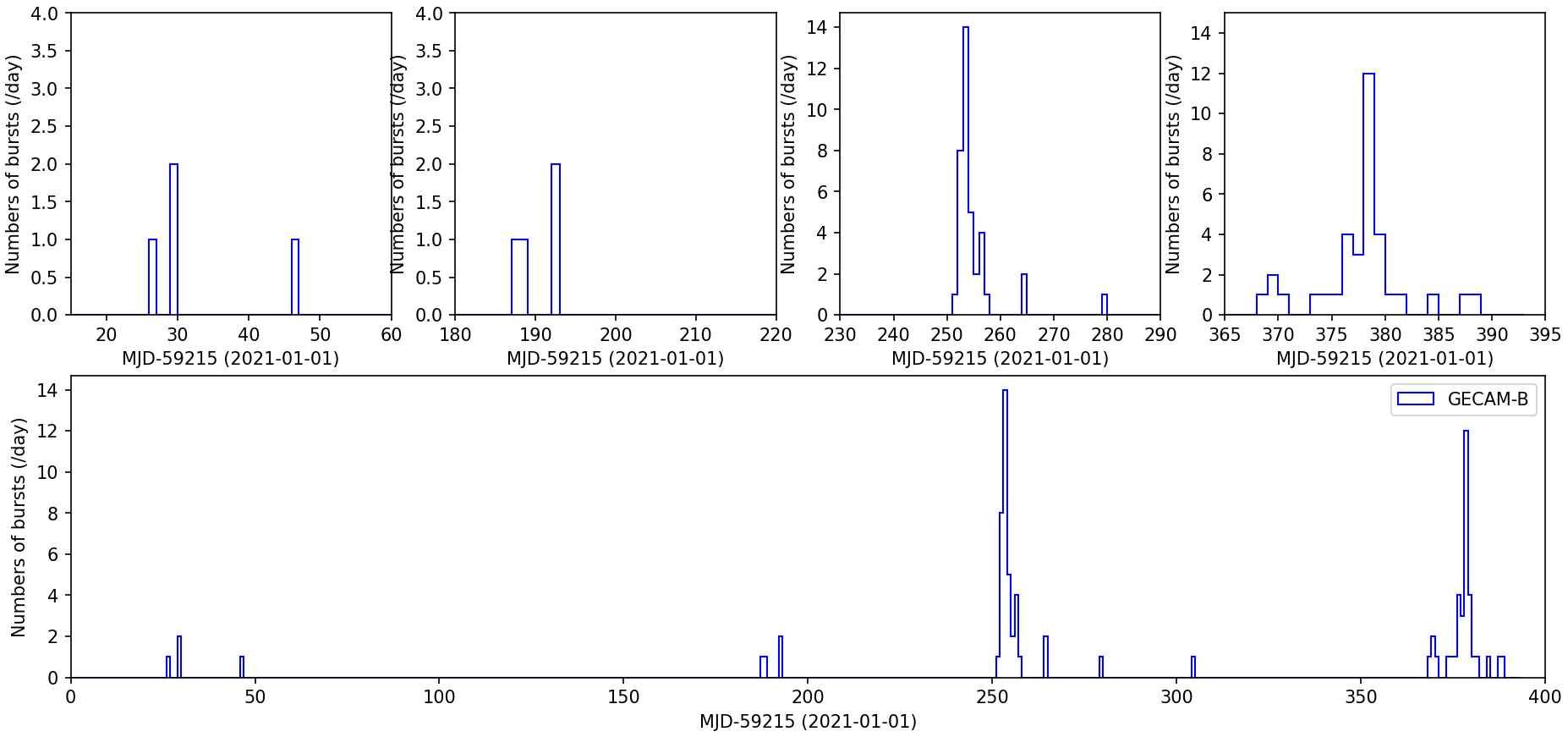
Figure 1: The burst history of SGR J1935+2154 from 2021 January to 2022 January.

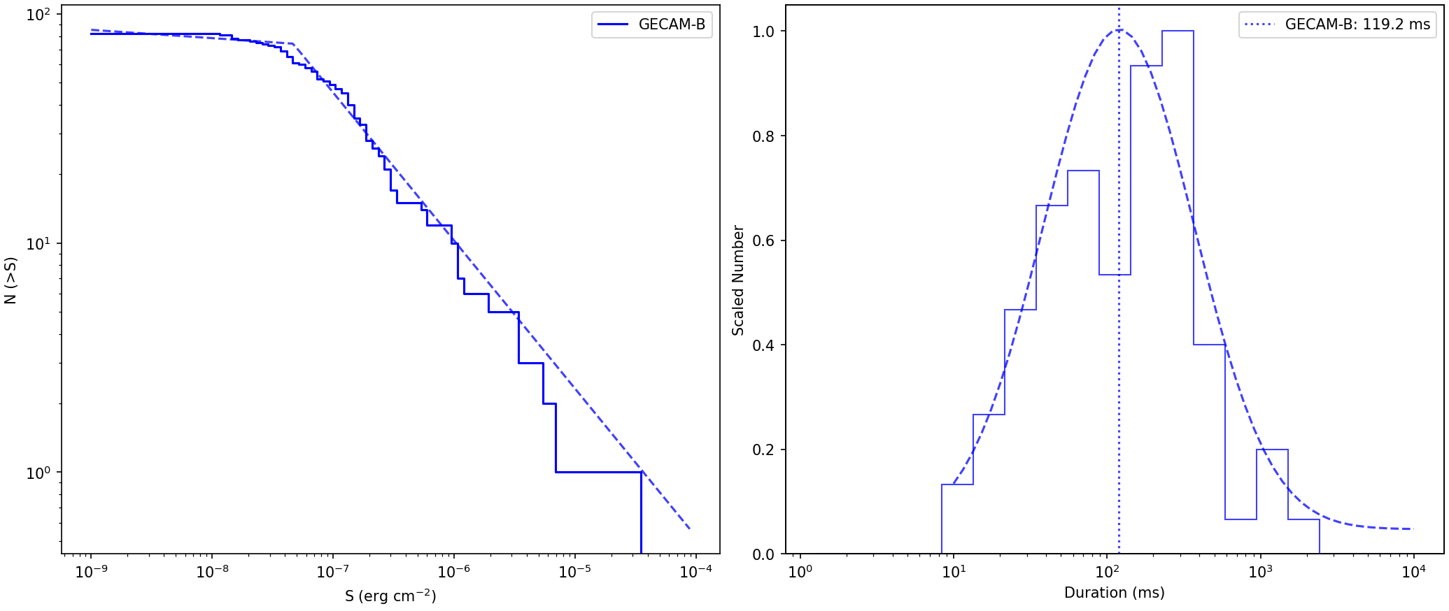
Figure 2: The left panel presents two complementary cumulative distributions of energy fluences of SGR J1935+2154 bursts over one year. The dashed lines represent the best-fit of the distribution using a broken power law. The right panel show the distribution of burst duration. The curve is Log-Gaussian function fits to the histogram and its central value is represented by vertical lines.

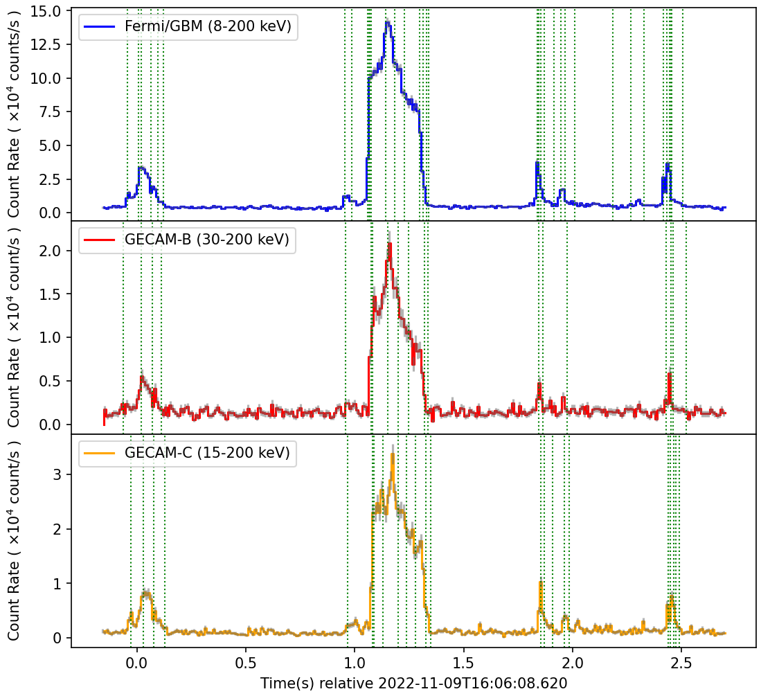
Figure 3: Example of the Bayesian Block analysis. The vertical green dashed lines are the Bayesian block edges.

2.2 Burst Hardness Ratio

The hardness ratio is the ratio of net counts of the source in different energy bands. The net counts is estimated as,

$$C=S-B$$ (1)

where $S$ and $B$ are the total counts and the expected background counts of the source. The background counts are estimated using total counts before and after the source time interval.

We compute the hardness ratio of each burst of the GECAM-B (H3/H2: 50-200 keV/30-50 keV), and the results are shown in Fig 4. The hardness ratios of these bursts range from 0.2 to 1.5, with a median value of 0.56. The left panel of Fig 4 represents the evolution of the hardness ratio and exhibits no significant trend. We also do not find a correlation between the duration and the hardness ratio (see the right panel of Fig 4).

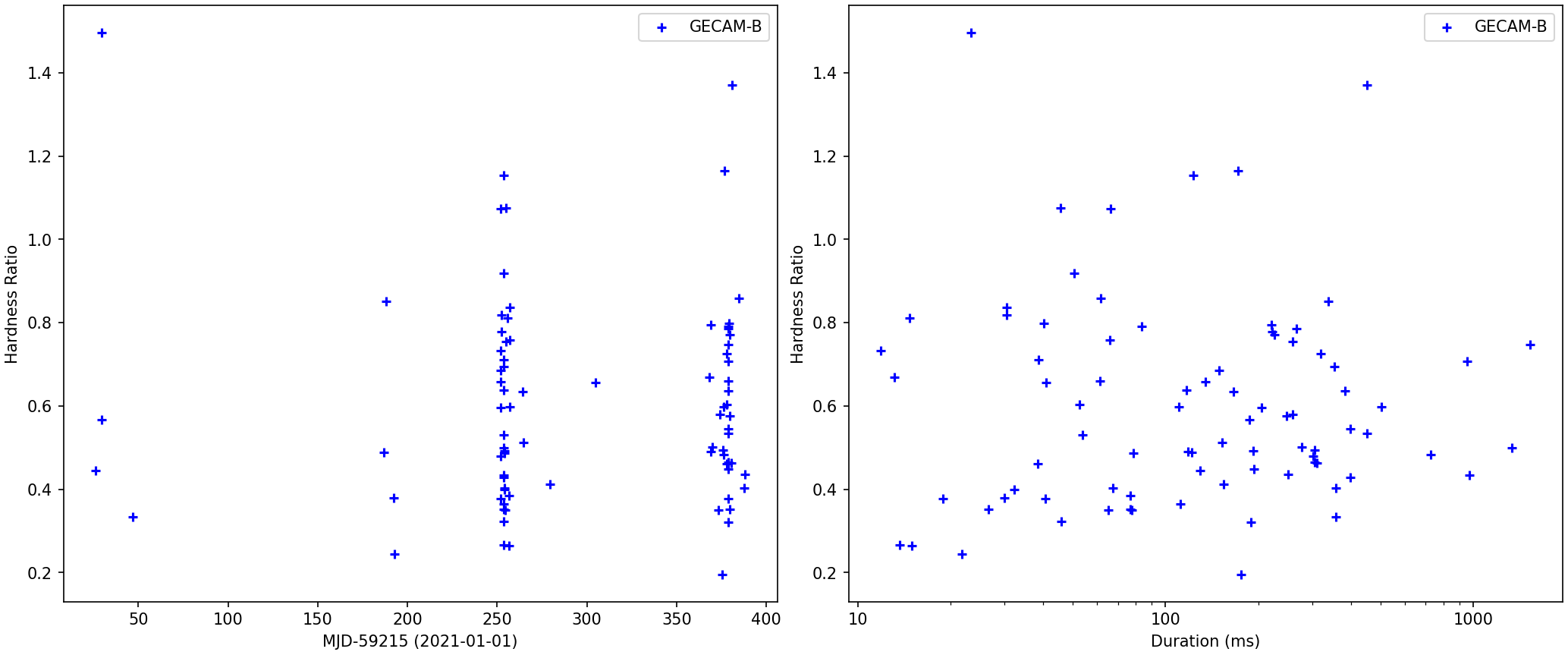
Figure 4: The left panel represents the evolution of the hardness ratio of the GECAM-B (H3/H2: 50-200 keV/30-50 keV). The right panel indicate the duration vs. hardness ratio of each burst.

3 Spectral Properties

A total of 82 bursts were observed by GECAM-B, of which 39 bursts were also observed by Fermi/GBM. Therefore, the dataset utilized in this study comprises of 82 GECAM-B bursts and 39 joint-spectra of both instruments (hereafter, GBM-GECAM). The GRD detectors, which are used in spectral fitting, with an angle to the source are less than $60^{\circ}$. The background spectra are accumulated from the data events during the preand post-burst time intervals (i.e., from T0 - 10s to T0 - 5 s and from T0 + 5s to T0 + 10 s, where T0 is the trigger time of the burst). For weak bursts, the GRPPHA command is used to group the observed data (e.g., GROUP MIN RCNTS) to ensure the validity of the fit statistics.

Then, we perform a time-integrated spectral analysis using the XSPEC (Arnaud, 1996) software and the Poisson data with Gaussian background statistics (PGSTAT). These burst samples are fitted with 6 models: a single Black Body (BB), a single Power Law (PL), an Optically-Thin Thermal Bremsstrahlung (OTTB), a single Black Body plus a single Power Law (BBPL), the Double Black Body (BB2) and an exponentially Cut-Off Power Law (CPL), over the energy range of 30-200 keV for GECAM-B and 8-200 keV for the GBM-GECAM. And finally, we use Bayesian Information Criterion (BIC, Schwarz, 1978; Liddle, 2007) to estimate the best-fit model among BB2, BB, CPL, OTTB, BBPL and PL.

One should note that the threshold of low energy for GECAM-B is dynamically changing over the course of this year. However, for consistency and the principle of controlling variables, the energy range for GECAM-B samples is set to 30-200 keV in all analyses conducted in this paper and in the localization research mentioned in Paper II. All results are presented in the Appendix A. The equations of these models are following:

The exponentially Cut-Off Power Law (CPL) model:

$$F(E)=K(\frac{E}{E_{\mathrm{piv}}})^{\alpha}e^{-(2+\alpha)E/E_{\mathrm{peak}}}$$ (2)

where $K$ is the amplitude in $\mathrm{photon/s/cm^{2}/keV}$, $E_{\mathrm{peak}}$ is the $\nu F_{\nu}$ peak in keV, $\alpha$ is the power-law index and $E_{\mathrm{piv}}$ is the pivot energy in keV and we set $E_{\mathrm{piv}}=20$ keV in this paper.

The Black Body (BB) model:

$$F(E)=\frac{1.0344\times 10^{-3}\times KE^{2}}{e^{E/kT}-1}$$ (3)

where $K$ is $R_{\mathrm{km}}^{2}/D_{10}^{2}$, $R_{\mathrm{km}}^{2}$ is the radiative area of source in km, $D_{10}^{2}$ is the distance to the source in units of 10 kpc and $kT$ is the temperature keV. We set the distance to the SGR J1935+2154 is 9 kpc in this paper.

The Optically-Thin Thermal Bremsstrahlung (OTTB) model:

$$F(E)=K(\frac{E_{\mathrm{piv}}}{E})e^{(E_{\mathrm{piv}}-E)/kT}$$ (4)

where $K$ is the amplitude in $\mathrm{photon/s/cm^{2}/keV}$ and $E_{\mathrm{piv}}$ is the pivot energy in keV and we set $E_{\mathrm{piv}}=20$ keV in this paper.

The Power Law (PL) model:

$$F(E)=KE^{\alpha}$$ (5)

where $K$ and $\alpha$ are same to the parameters of CPL model.

3.1 Burst Fluence

The fluence is derived from the product of the burst duration and the flux, and the flux is calculated using the best-fit model in the energy ranges of 30-200 keV for GECAM-B samples. The results are listed in Appendix A.

The left panel of Fig 2 shows the complementary cumulative distribution of energy fluences, which can be fitted by a broken power law. The break point is $4.69\pm 0.17\times 10^{-8}\ \mathrm{erg\cdot cm^{-2}}$ for GECAM-B samples. The slope of the lower fluences is $-0.036\pm 0.004$. The slope of the higher fluences is $-0.65\pm 0.02$. The slope of higher fluences are consistent with the previous studies (Collazzi et al., 2015; Cheng et al., 1996; Lin et al., 2020b, a; Rehan & Ibrahim, 2023) and the Gutenberg-Richter law ($N(E)\propto E^{-5/3\sim-2}$), which describes the power-law-like frequency distribution of earthquakes. This similarity implies that the majority magnetar bursts, akin to earthquakes, possibly originated from the cracks in the solid crust of the magnetar (Duncan & Thompson, 1992).

3.2 The Double Black Body Model

The Double Black Body Model (BB2) is the sum of two BBs (Eq 3). Of all burst samples, 41 GECAM-B bursts and 19 GBM-GECAM bursts can be well-fitted with the BB2 model. The Fig 5 shows the distribution of the low- and the high-temperature ($kT_{\mathrm{low}}$, $kT_{\mathrm{high}}$) of BB2. Both $kT_{\mathrm{low}}$ and $kT_{\mathrm{high}}$, respectively, can be well fit with a Gaussian function (see Table 2 for central value and sigma). The BB2 temperature distribution of GBM-GECAM samples is similar to that of SGR J1935+2154 in previous erports (Lin et al., 2020b, a; Rehan & Ibrahim, 2023).

The Fig 6 represents that $kT_{\mathrm{low}}$ and $kT_{\mathrm{high}}$ exhibit a strong Log-Linear correlation to the emission area ($R_{\mathrm{low}}$, $R_{\mathrm{high}}$), and the results are listed in Table 1. In addition, the emission area dependence spanning both the low and high BB temperatures, namely $R_{\mathrm{both}}^{2}\propto(kT_{\mathrm{both}})^{-4.23\pm 0.15}$ for GECAM-B samples and $R_{\mathrm{both}}^{2}\propto(kT_{\mathrm{both}})^{-3.60\pm 0.13}$, is very similar to the one corresponding to a single BB obeying the Stefan-Boltzmann law: $R^{2}\propto(kT)^{-4}$. This $R^{2}-kT$ correlation for BB2 model is also similar to that observed for the collection of SGR J1550-5418 bursts analyzed in previous studies (Lin et al., 2012; van der Horst et al., 2012).

Because of the limited sample size, there are some differences between the correlation results of GECAM-B and GBM-GECAM. The correlation ($R_{\mathrm{low}}^{2}\propto(kT_{\mathrm{low}})^{\alpha}$) of GECAM-B bursts exhibits a steeper trend since the higher fitted lower-edge energy range (30-200 keV). This is also the reason why the BB/BB2 temperature distribution of GBM-GECAM is different from that of GECAM-B, and will be discussed in Subsection 3.5.

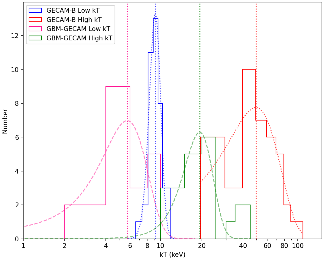
Figure 5: The temperature distributions of the BB2 model of GECAM-B and GBM-GECAM.

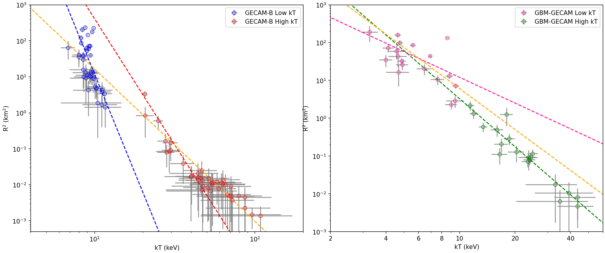
Figure 6: The left panel is the emission areas ($R^{2}$) as a function of the low- and the high-temperature of the BB2 model of GECAM-B. The right panel is the emission areas ($R^{2}$) as a function of the low- and the high-temperature of the BB2 model of GBM-GECAM.

Table 1: The measure results of the Spearman’s rank correlation coefficient.

Correlation	PL Index ($\alpha$)	Coefficien ($\rho$)	p-value	Instrument
$R_{\mathrm{low}}^{2}\propto(kT_{\mathrm{low}})^{\alpha}$	-10.92 $\pm$ 0.10	-0.63	1.03E-05	GECAM-B
$R_{\mathrm{high}}^{2}\propto(kT_{\mathrm{high}})^{\alpha}$	-7.01 $\pm$ 0.39	-0.92	1.08E-17	GECAM-B
$R_{\mathrm{both}}^{2}\propto(kT_{\mathrm{both}})^{\alpha}$	-4.23 $\pm$ 0.15	-0.94	3.33E-40	GECAM-B
$R_{\mathrm{low}}^{2}\propto(kT_{\mathrm{low}})^{\alpha}$	-2.26 $\pm$ 0.80	-0.66	2.28E-03	GBM-GECAM
$R_{\mathrm{high}}^{2}\propto(kT_{\mathrm{high}})^{\alpha}$	-4.22 $\pm$ 0.84	-0.91	8.56E-08	GBM-GECAM
$R_{\mathrm{both}}^{2}\propto(kT_{\mathrm{both}})^{\alpha}$	-3.60 $\pm$ 0.13	-0.91	8.56E-08	GBM-GECAM

Table 2: The Gaussian distribution of the spectral parameters

Model	Parameter	$\mu$	$\sigma$	Instrument
BB2	$kT_{\mathrm{low}}$ (keV)	9.16	0.88	GECAM-B
BB2	$kT_{\mathrm{high}}$ (keV)	49.56	23.17	GECAM-B
BB2	$kT_{\mathrm{low}}$ (keV)	5.72	2.21	GBM-GECAM
BB2	$kT_{\mathrm{high}}$ (keV)	19.30	4.70	GBM-GECAM
CPL	$\alpha$	-1.21	0.33	GBM-GECAM
CPL	$E_{\mathrm{peak}}$ (keV)	34.26	8.59	GBM-GECAM
BBPL	kT (keV)	9.18	1.30	GECAM-B
BBPL	$\alpha$	-1.20	0.37	GECAM-B
BBPL	kT (keV)	8.82	0.52	GBM-GECAM
BBPL	$\alpha$	-2.16	0.13	GBM-GECAM
BB	kT (keV)	8.74	0.58	GBM-GECAM
BB	kT (keV)	18.15	8.77	GECAM-B
OTTB	kT (keV)	35.83	10.22	GBM-GECAM
OTTB	kT (keV)	54.02	11.91	GECAM-B
PL	$\alpha$	-2.14	0.24	GBM-GECAM
PL	$\alpha$	-2.06	0.63	GECAM-B
MBB	$\beta$	5.65	0.44	GBM-GECAM
MBB	$\beta$	5.11	0.46	GECAM-B
MBB	$kT_{\mathrm{min}}$	4.47	1.55	GBM-GECAM
MBB	$kT_{\mathrm{min}}$	5.16	1.83	GECAM-B

3.3 The Cut-Off Power Law model

As for the CPL model (Eq 2), 5 GECAM-B bursts and 24 GBM-GECAM bursts can be well-fitted. If the low energy edge of GECAM-B bursts is greater than $\sim$30 keV, it becomes difficult to effectively constrain the CPL model. As a result, only a limited number of bursts can be successfully fitted using this model. The CPL model is not recommended for fitting SGR burst data observed by GECAM-B, especially there is a possibility of the low energy edge increasing in future operations, or other instruments with a similar energy range. The distributions of $\alpha$ and $E_{\mathrm{peak}}$ are presented in the upper two panels of Fig 7. The the GBM-GECAM distributions can be fitted with a Gaussian function (see Table 2 for central value and sigma).

Most of $E_{\mathrm{peak}}$ values range from approximately 20 to 60 keV. The distributions of the two parameters are similar to those in previous studies. However, the correlation between the $\alpha$ and the fluence, as well as the relation between the $E_{\mathrm{peak}}$ and the fluence exhibit weak relevance, as shown in the lower two panels of Fig 7.

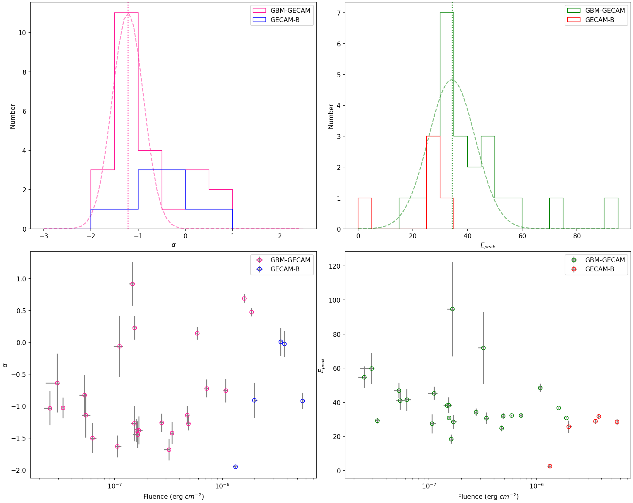
Figure 7: The upper two panels present distributions of the CPL model parameters ($\alpha$ and $E_{\mathrm{peak}}$) of the GECAM-B and the GBM-GECAM. The curves are Gaussian fits to the histograms and their central values are represented by vertical lines. The lower two panels show the relevance between the $\alpha$ and the $E_{\mathrm{peak}}$ to the fluence.

3.4 The Other Models

The Fig 8 represents the parameters histogram distribution of the BBPL (the sum of Eq 3 and Eq 5), OTTB (Eq 4), BB (Eq 3), and PL (Eq 5) models. The distributions can be fitted with a Gaussian function (see Table 2 for central value and sigma). The $kT$ of the BBPL is similar to that of the BB, and the Photon Index ($\alpha$) of the BBPL is similar to that of the PL. The $kT$ of the OTTB is similar to the $E_{\mathrm{peak}}$ of the CPL since the $kT$ of the OTTB is equivalent to $E_{\mathrm{peak}}$ of the CPL ($\alpha$=-1). The BB/OTTB models in GECAM-B and GBM-GECAM have different $kT$ values, which can be attributed to differences in the energy range used for fitting.

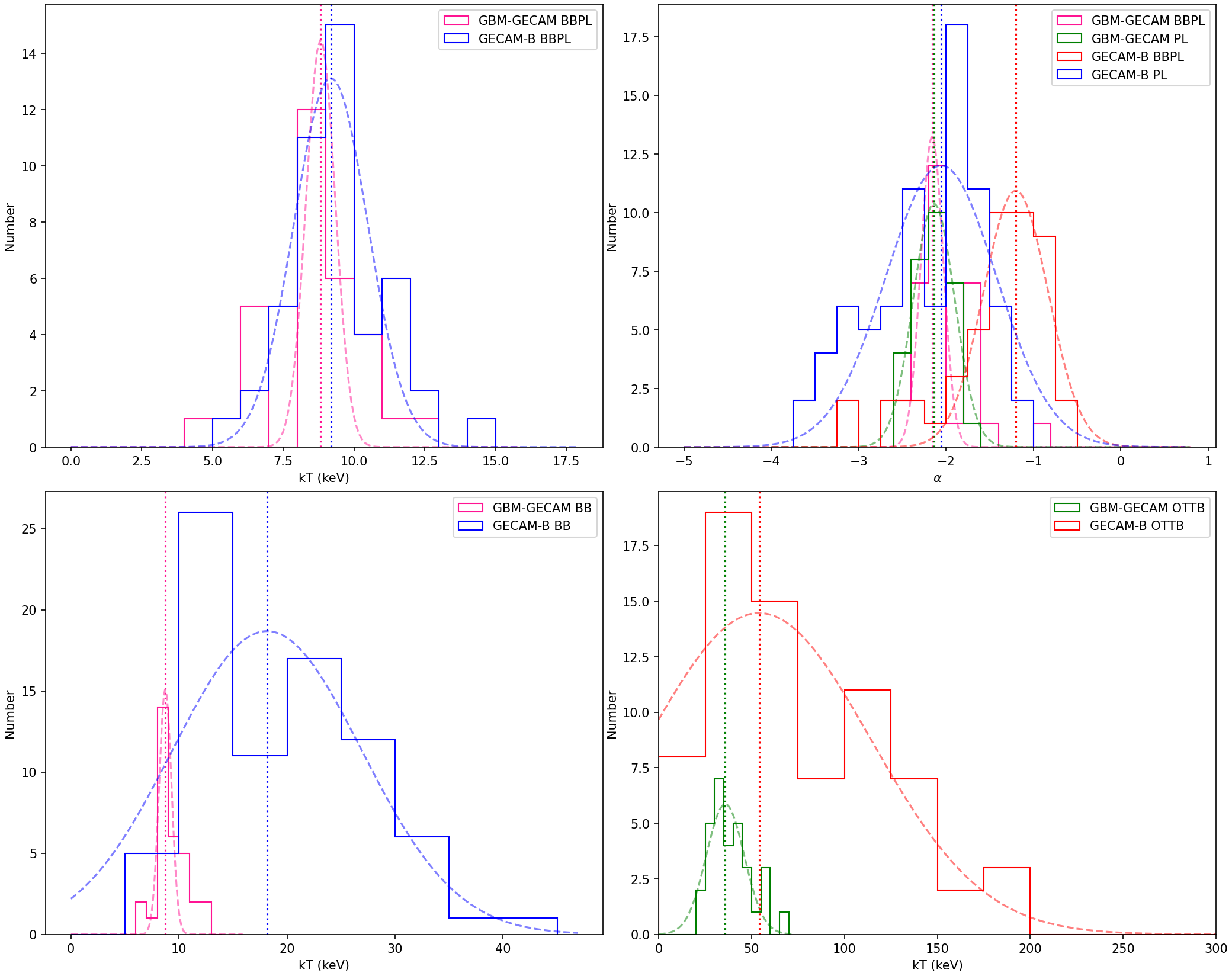
Figure 8: The distributions of the BBPL, OTTB, BB, and PL models parameters of the GECAM-B and the GBM-GECAM.

3.5 The Multi-Temperature Black Body

The $kT$ distribution of the BB2/BB models as observed by GECAM-B differs from that of GBM-GECAM samples due to differences in the energy range used for fitting. Thus we assume the SGR bursts consist of multiple Black Bodies (BBs), and the temperatures of these BBs follow a power law distribution as following,

$$f(kT)=kT^{-\beta}$$ (6)

Then we perform integration of Eq (6) from $kT_{\mathrm{min}}$ to infinity. The spectrum is defined as,

$$N(E)=K\int_{kT_{\mathrm{min}}}^{\infty}f(kT)\frac{E^{2}}{\exp(\frac{E}{kT})-1}d(kT)$$ (7)

where $K$, $\beta$ and $kT_{\mathrm{min}}$ are normalization coefficient, power law $kT$ index and Minimum temperature.

The fit results are shown/listed in Fig 9 and Appendix A. The $\beta$ and $kT_{\mathrm{min}}$ distributions of GECAM-B and GBM-GECAM are similar to each other representing that they originated from similar thermal radiation even different $kT$ distribution of the BB2/BB models. Therefore, the MBB model is recommended for analyzing the BB temperature of magnetar bursts, even when using different instruments with similar detection energy ranges.

As shown in the right panel of Fig 10, the $kT$ of BB model exhibit a Log-Linear correlation to the $\beta$ of MBB model. We fit the correlation ($\beta\propto kT$) with a simple power law function using both GECAM-B and GBM-GECAM samples, and obtain the slope: $-0.25\pm 3\mathrm{E}-16$. This indicates that the higher temperature of the BB model corresponds to a wider temperature distribution, ranging from $kT_{\mathrm{min}}$ to an even higher temperature, as we expected. The left panel of Fig 10 show the correlation between $\beta$ and $kT_{\mathrm{min}}$. The correlation ($\beta\propto kT_{\mathrm{min}}$) is also fitted by a power law function, which give the slope: $0.11\pm 1.3\mathrm{E}-14$. However, the correlation between $\beta$ and burst fluence/duration, as well as the relation between $kT_{\mathrm{min}}$ and burst fluence/duration exhibit weak relevance, as shown in the Fig 11.

Interesting, The temperature values ($kT_{\mathrm{min}}\sim 5$ keV) of the MBB model are similar to those of the Multicolor Blackbody model (Hou et al., 2018), which describes a superposition of a series of Black Bodies with different temperatures for GRB 081221. Compared to GRB 081221, the slope ($\beta\sim 5.5$) of the temperature distribution indicates a narrow temperature distribution. This is because magnetar bursts are generally softer than typical GRBs.

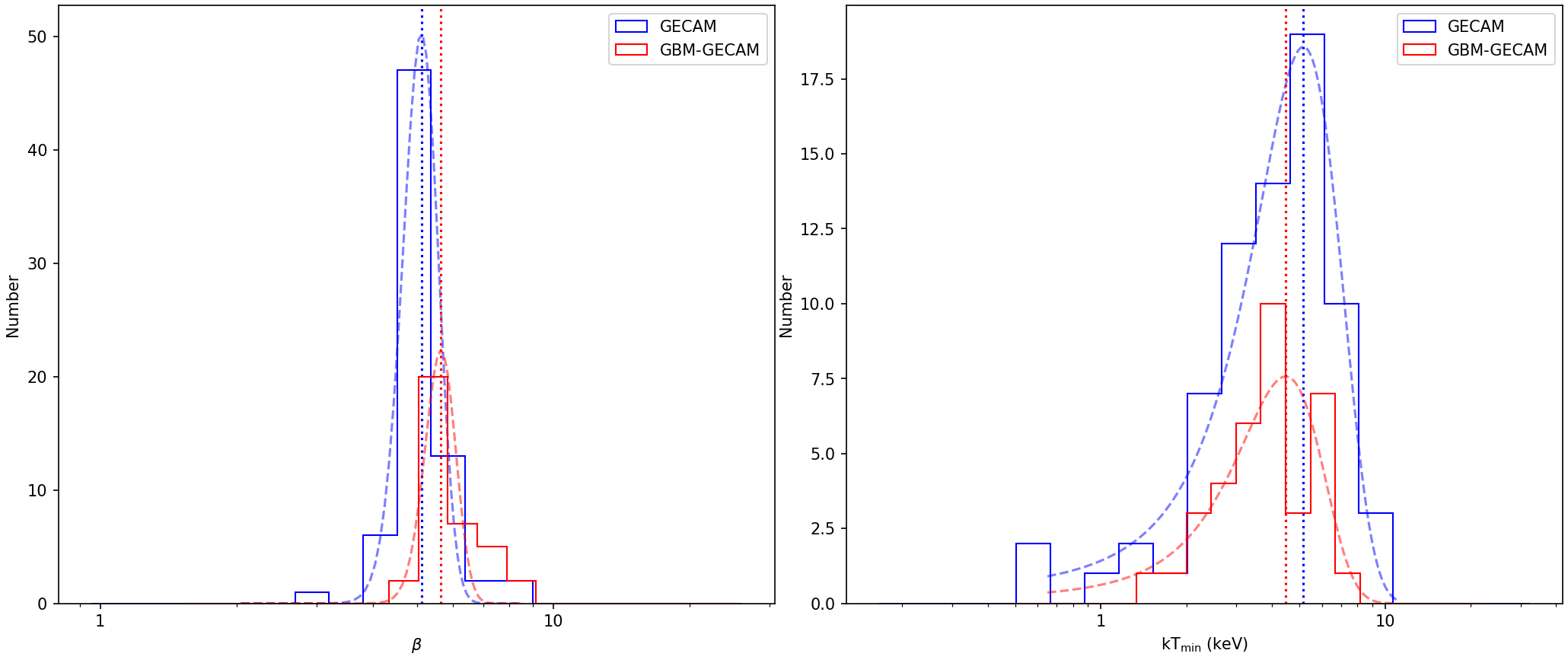
Figure 9: The left and right panels are the $\beta$ and $kT_{\mathrm{min}}$ distributions of the MBB model, respectively.

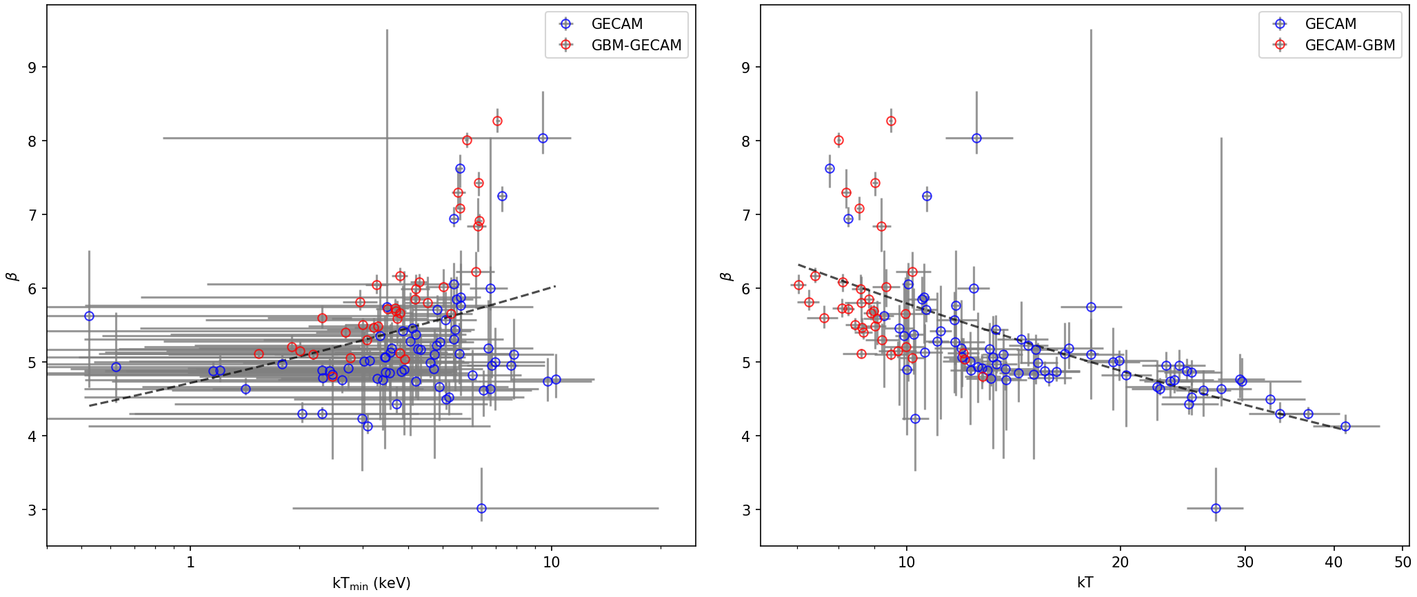
Figure 10: The left panel presents the $kT_{\mathrm{min}}$ vs. $\beta$ of each burst. The right panel presents the temperature ($kT$) of BB model vs. $\beta$ of MBB model for each burst.

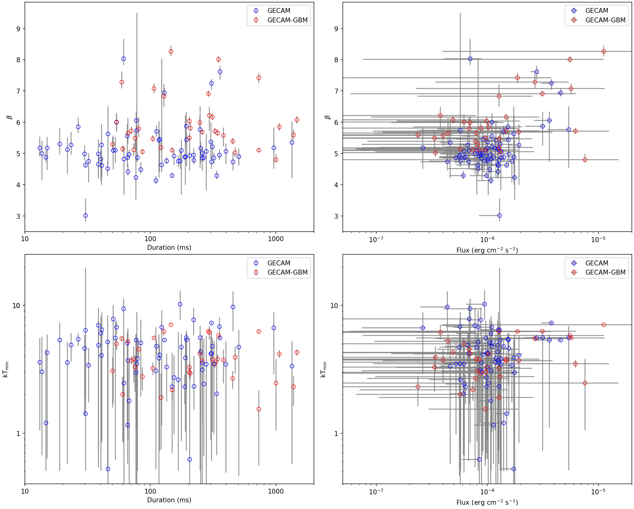
Figure 11: The upper two panels present the correlation between $\beta$ and burst duration/flux. The lower two panels present the correlation between $\beta$ and burst duration/flux.

3.6 Time-Resolved Spectral Analysis

GECAM-C, a gamma-ray monitor akin to GECAM-B, was launched on July 2022, aboard the SATech-01 satellite (Zhang et al., 2023). To examine the observation capabilities of GECAM-C on magnetar, we also conduct a spectral analysis of a burst detected by Fermi/GBM, GECAM-B, and GECAM-C, as shown in Fig 3. We chose this burst for analysis because of the approaching detection energy range of the three instruments and had significant burst fluence. However, one should note that this burst is just for exhibiting the spectral analysis of GECAM-C and is not contained in the above statistical analysis (2021-01 to 2022-01).

We generate the spectral dataset based on Bayesian block edges and correct the time delays of such three instruments in order to perform joint-spectra fitting, as shown in the left side of Fig 12. The right panel of Fig 12 is a time-integrated spectral fitting with the CPL model ($E_{\mathrm{{peak}}}=29.85\pm 0.34$ keV, $\alpha=-0.12\pm 0.08$).

We conduct a separate spectral analysis using GECAM-C for localization research, and the results show that the localization is close to the true position. For more detailed spectral fitting and localization results, please refer to Paper II.

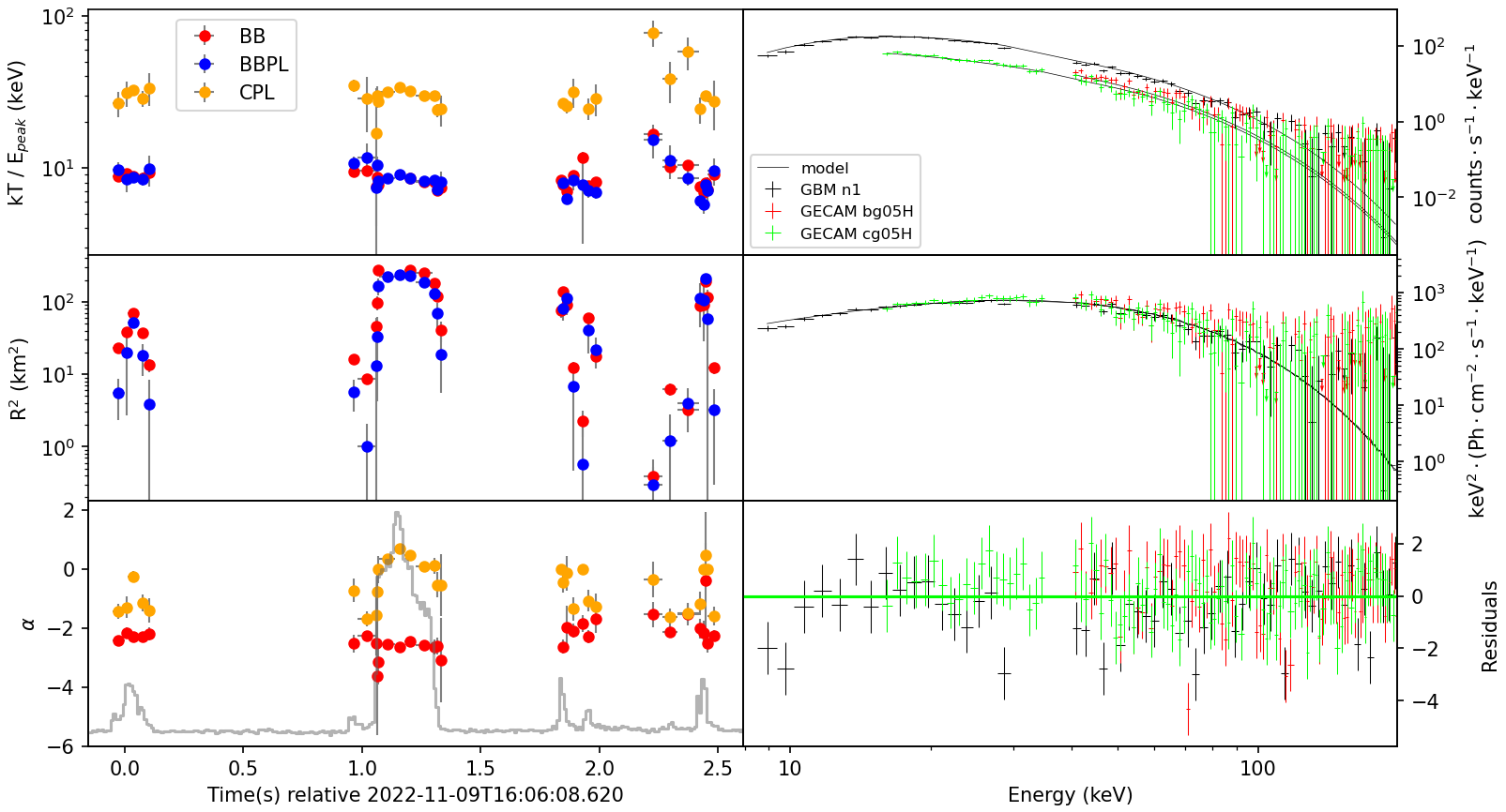
Figure 12: The left panel is the $kT$/$E_{\mathrm{peak}}$/$\alpha$ evolution as a function of time. The right panel is the time-integrated spectral fitting with the CPL model.

4 Summary

In this paper, we make the temporal and spectral analysis based on GECAM-B EVT dates from January 2021 through January 2022, which is also helpful to study the localization (see Paper II). Fig 1 exhibit multiple active burst episodes of SGR J1935+2154 over this year.

The left panel of Fig 2 represents the cumulative distribution of the fluence can be well fitted by broken power law. The break point is $4.69\pm 0.17\times 10^{-8}\ \mathrm{erg\cdot cm^{-2}}$ for GECAM-B samples. The slope of the lower fluences is $-0.036\pm 0.004$. The slope of the higher fluences is $-0.65\pm 0.02$. The bursts duration follow a Log-Gaussian distribution with a central value of 119.2 ms, as shown in the right panel of Fig 2. The burst duration mentioned above are computed by the Bayesian Block method. The hardness ratio is computed in different energy ranges (H3/H2: 50-200 keV/30-50 keV for GECAM-B) and shown in Fig 4. The hardness ratio is range from 0.2 to 1.5, with a median value of 0.56.

The fluence mentioned above is derived from the product of the burst duration and the flux. The flux is calculated by the best-fit model, which is assessed by spectral fitting. We carry out a time-integrated spectral analysis using the PGSTAT statistics with BB2, CPL, BBPL, OTTB, BB, and PL models. The distributions of each model parameter ($kT$, $E_{\mathrm{peak}}$ or $\alpha$) follow a Gaussian distribution which the central value is listed in Table 2. As for the BB2 model, the emission area exhibits a Log-Linear correlation with each corresponding temperature (see Fig 6). As for the CPL model, we do not find correlation between the fluence and the $E_{\mathrm{peak}}$, and the relation between the fluence and the Photon Index ($\alpha$). The CPL model is not recommended for fitting SGR burst data observed by GECAM-B, especially there is a possibility of the low energy edge increasing in future operations, or other instruments with a low energy threshold higher than 30 keV.

To investigate the thermal radiation emitted during a magnetar burst, we assume the temperature of Black Bodies (BBs) follows a power law distribution, as described in Eq 6. Based on this assumption, the spectrum is Eq 7. We perform a fit of the spectrum using all available datasets, and find that a total of 82 GECAM bursts and 39 GBM-GECAM bursts could be well-fit using this MBB model. As shown in Fig 9, the concentration of $kT_{\mathrm{min}}$ values in our analysis indicate that magnetar burst spectra tend to be soft and may be composed of multiple BB components. The steep slope ($\beta$) of the temperature distribution further suggests that the majority of the BB temperatures are concentrated around the concentrated around 5 keV. Additionally, the $\beta$ and $kT_{\mathrm{min}}$ distributions of GECAM-B and GBM-GECAM are similar to each other representing that the MBB model is recommended for analyzing the BB temperature of magnetar bursts, even when using different instruments with similar detection energy ranges. This finding provides important insights into the thermal properties of magnetars, and can help inform future studies of these fascinating objects.

This work is supported by the National Key R&D Program of China (2021YFA0718500), the National Natural Science Foundation of China (Grant No. 11833003, 12273042) and the National SKA program of China (2020SKA0120300). The GECAM (Huairou-1) mission is supported by the Strategic Priority Research Program on Space Science (Grant No. XDA15360000, XDA15360102, XDA15360300) of the Chinese Academy of Sciences.

Appendix A Temporal and Spectral Properties of SGR J1935+2154

Table 3: The temporal properties of SGR J1935+2154 observed by GECAM-B

ID	UTC	Duration (ms)	Model	Fluence	ID	UTC	Duration (ms)	Model	Fluence
1	2021-01-27T06:50:20.750	129.17	PL	$45.6_{-3.29}^{+0.75}$	42	2021-09-14T23:26:34.050	30.37	PL	$12.85_{-4.45}^{+0.12}$
2	2021-01-30T08:39:53.840	187.36	PL	$6.34_{-2.57}^{+0.15}$	43	2021-09-15T02:39:25.700	65.87	PL	$11.36_{-3.81}^{+0.09}$
3	2021-01-30T10:35:35.120	23.29	OTTB	$6.64_{-1.13}^{+0.39}$	44	2021-09-22T02:39:10.200	166.41	PL	$5.73_{-2.74}^{+0.16}$
4	2021-02-16T22:20:39.600	357.11	BBPL	$27.79_{-3.35}^{+0.41}$	45	2021-09-22T20:12:16.500	152.61	BBPL	$72.8_{-12.07}^{+1.61}$
5	2021-07-07T00:33:31.640	121.92	BB2	$83.98_{-11.97}^{+0.26}$	46	2021-10-07T11:57:07.700	153.99	PL	$9.77_{-1.74}^{+0.21}$
6	2021-07-08T00:18:18.560	337.3	PL	$6.08_{-1.52}^{+0.11}$	47	2021-11-01T23:13:41.950	40.93	PL	$12.56_{-3.83}^{+0.01}$
7	2021-07-12T04:32:39.600	29.92	PL	$15.56_{-6.59}^{+0.13}$	48	2022-01-04T04:32:11.200	13.16	PL	$11.74_{-11.74}^{+0.02}$
8	2021-07-12T22:12:58.100	21.84	BBPL	$12.63_{-5.89}^{+0.72}$	49	2022-01-05T06:01:31.450	220.58	PL	$8.76_{-2.24}^{+0.03}$
9	2021-09-09T21:07:12.150	204.57	PL	$8.44_{-2.52}^{+0.09}$	50	2022-01-05T07:06:40.800	118.15	BB2	$9.15_{-3.9}^{+0.0}$
10	2021-09-10T01:04:33.500	11.9	PL	$15.01_{-7.67}^{+0.31}$	51	2022-01-06T02:36:14.100	277.75	PL	$13.24_{-1.65}^{+0.19}$
11	2021-09-10T02:07:56.700	66.12	PL	$12.47_{-3.34}^{+0.01}$	52	2022-01-09T07:39:10.700	65.3	PL	$10.96_{-4.98}^{+0.08}$
12	2021-09-10T02:08:28.800	134.65	PL	$10.04_{-3.13}^{+0.14}$	53	2022-01-10T06:52:40.500	258.9	PL	$8.61_{-1.9}^{+0.32}$
13	2021-09-10T03:22:40.550	302.12	PL	$10.06_{-1.96}^{+0.26}$	54	2022-01-11T08:58:35.450	176.2	PL	$8.06_{-2.55}^{+0.09}$
14	2021-09-10T03:24:47.150	40.72	PL	$19.26_{-3.95}^{+0.29}$	55	2022-01-12T01:03:46.900	304.94	PL	$6.77_{-1.71}^{+0.11}$
15	2021-09-10T03:42:45.750	148.83	PL	$9.78_{-2.88}^{+0.31}$	56	2022-01-12T05:42:51.650	503.61	PL	$5.61_{-1.91}^{+0.11}$
16	2021-09-10T05:05:03.350	221.65	PL	$12.7_{-2.39}^{+0.02}$	57	2022-01-12T08:39:25.450	728.17	BBPL	$52.9_{-5.56}^{+0.27}$
17	2021-09-10T05:35:55.500	30.41	PL	$14.89_{-2.88}^{+0.1}$	58	2022-01-12T17:57:08.500	172.48	PL	$9.45_{-3.05}^{+0.11}$
18	2021-09-11T16:39:21.000	50.54	PL	$6.85_{-6.85}^{+0.19}$	59	2022-01-13T19:36:08.600	52.61	PL	$9.65_{-3.81}^{+0.4}$
19	2021-09-11T16:50:03.850	45.88	PL	$17.25_{-4.28}^{+0.04}$	60	2022-01-13T20:14:58.600	319.95	PL	$5.2_{-1.56}^{+0.06}$
20	2021-09-11T17:01:10.800	974.33	BB2	$76.89_{-2.92}^{+0.35}$	61	2022-01-13T21:41:17.900	38.46	PL	$12.36_{-5.5}^{+0.0}$
21	2021-09-11T17:04:29.800	13.65	PL	$8.94_{-5.07}^{+0.04}$	62	2022-01-14T19:42:08.050	193.26	PL	$15.52_{-2.11}^{+0.18}$
22	2021-09-11T17:10:48.750	398.48	PL	$6.14_{-2.03}^{+0.02}$	63	2022-01-14T19:45:08.100	18.93	PL	$13.05_{-9.02}^{+0.07}$
23	2021-09-11T18:02:13.500	38.57	PL	$7.72_{-3.97}^{+0.13}$	64	2022-01-14T19:56:52.700	382.4	BB2	$147.37_{-5.45}^{+0.33}$
24	2021-09-11T18:04:46.350	354.67	PL	$5.65_{-1.42}^{+0.16}$	65	2022-01-14T20:06:07.400	83.6	PL	$10.5_{-3.38}^{+0.32}$
25	2021-09-11T18:54:36.050	26.54	PL	$15.33_{-5.56}^{+0.33}$	66	2022-01-14T20:07:03.050	452.02	BB2	$45.28_{-5.07}^{+0.04}$
26	2021-09-11T19:43:28.000	116.83	PL	$11.94_{-2.63}^{+0.06}$	67	2022-01-14T20:12:45.300	957.86	PL	$2.63_{-1.89}^{+0.15}$
27	2021-09-11T19:46:50.050	53.73	PL	$10.97_{-6.05}^{+0.15}$	68	2022-01-14T20:15:54.400	305.94	BBPL	$37.84_{-7.35}^{+0.86}$
28	2021-09-11T20:13:40.550	111.79	PL	$14.03_{-2.67}^{+0.27}$	69	2022-01-14T20:21:05.150	1530.34	BB2	$239.77_{-2.79}^{+0.42}$
29	2021-09-11T20:22:59.050	1334.24	PL	$4.63_{-0.91}^{+0.04}$	70	2022-01-14T20:23:35.400	189.16	PL	$17.39_{-2.87}^{+0.08}$
30	2021-09-11T20:33:14.550	123.12	PL	$8.23_{-2.99}^{+0.15}$	71	2022-01-14T20:26:50.300	61.19	PL	$6.98_{-2.94}^{+1.89}$
31	2021-09-11T22:51:41.600	78.74	PL	$13.34_{-3.45}^{+0.22}$	72	2022-01-14T20:29:07.250	398.07	BBPL	$28.81_{-6.74}^{+0.69}$
32	2021-09-12T00:34:37.450	192.29	BBPL	$31.48_{-9.65}^{+1.54}$	73	2022-01-14T20:31:49.900	265.8	PL	$6.2_{-2.02}^{+0.02}$
33	2021-09-12T00:45:49.400	32.17	PL	$16.6_{-3.54}^{+0.12}$	74	2022-01-15T09:26:39.900	40.19	PL	$10.81_{-5.61}^{+0.23}$
34	2021-09-12T05:14:07.950	67.48	PL	$10.73_{-2.28}^{+0.17}$	75	2022-01-15T13:52:26.050	76.73	BB2	$17.62_{-7.87}^{+0.52}$
35	2021-09-12T16:26:08.150	77.84	PL	$5.71_{-3.26}^{+0.03}$	76	2022-01-15T16:31:14.900	225.69	PL	$7.44_{-2.58}^{+0.28}$
36	2021-09-12T22:16:36.200	45.55	PL	$8.25_{-3.82}^{+0.29}$	77	2022-01-15T17:21:59.300	247.88	BBPL	$53.91_{-19.11}^{+0.17}$
37	2021-09-13T00:27:25.200	258.7	BB2	$8.84_{-4.83}^{+0.42}$	78	2022-01-16T10:48:37.650	310.99	BBPL	$10.99_{-6.84}^{+0.58}$
38	2021-09-13T19:51:33.350	14.69	PL	$14.02_{-4.98}^{+0.01}$	79	2022-01-17T01:39:37.300	452.21	PL	$4.37_{-1.88}^{+0.14}$
39	2021-09-14T11:10:36.250	76.83	BBPL	$36.07_{-9.73}^{+1.94}$	80	2022-01-20T18:52:48.950	61.4	PL	$10.19_{-4.13}^{+0.3}$
40	2021-09-14T14:15:42.900	15.02	PL	$9.99_{-9.99}^{+0.27}$	81	2022-01-23T20:06:38.750	358.16	BB2	$99.96_{-4.15}^{+0.09}$
41	2021-09-14T23:21:58.500	110.27	PL	$10.8_{-2.86}^{+0.34}$	82	2022-01-24T02:10:55.050	250.47	PL	$12.43_{-2.22}^{+0.23}$

Table 4: The spectral properties of BB2 and BB model observed by GECAM-B

ID	BB2					BB
	kT1 (keV)	norm1	kT2 (keV)	norm2	PGSTAT/DOF	kT (keV)	norm	PGSTAT/DOF
1	$8.22_{-0.31}^{+0.31}$	$149.66_{-26.17}^{+26.17}$	$27.61_{-3.01}^{+3.01}$	$0.21_{-0.12}^{+0.12}$	198.06/206	$10.16_{-0.17}^{+0.17}$	$60.58_{-5.07}^{+5.07}$	321.83/208
2	$11.64_{-3.01}^{+3.01}$	$1.76_{-1.29}^{+1.42}$	$39.79_{-12.66}^{+14.85}$	$0.02_{-0.02}^{+0.03}$	109.66/171	$23.95_{-1.53}^{+1.53}$	$0.19_{-0.05}^{+0.05}$	123.31/173
3	…	…	…	…	…	$17.78_{-1.55}^{+1.55}$	$0.65_{-0.24}^{+0.24}$	72.98/109
4	$8.25_{-0.19}^{+0.16}$	$106.52_{-12.92}^{+12.92}$	$86.62_{-37.63}^{+37.63}$	$0.00_{-0.00}^{+0.00}$	228.08/238	$8.83_{-0.17}^{+0.17}$	$77.47_{-7.48}^{+7.48}$	358.63/240
5	$8.37_{-0.34}^{+0.34}$	$256.75_{-42.26}^{+42.26}$	$20.64_{-2.59}^{+2.59}$	$1.04_{-0.78}^{+0.78}$	199.34/199	$10.02_{-0.14}^{+0.14}$	$124.19_{-8.50}^{+8.50}$	281.15/201
6	…	…	…	…	…	$35.64_{-2.73}^{+2.73}$	$0.05_{-0.01}^{+0.01}$	235.67/200
7	…	…	…	…	…	$20.85_{-1.08}^{+1.08}$	$0.80_{-0.16}^{+0.16}$	145.91/159
8	$7.96_{-0.78}^{+0.78}$	$45.29_{-22.61}^{+22.61}$	$86.47_{-39.88}^{+48.48}$	$0.01_{-0.01}^{+0.01}$	97.09/111	$12.30_{-0.69}^{+0.69}$	$7.08_{-1.82}^{+1.82}$	170.42/113
9	$11.52_{-1.34}^{+1.34}$	$4.24_{-1.96}^{+1.96}$	$47.12_{-19.37}^{+19.37}$	$0.01_{-0.01}^{+0.02}$	128.47/153	$15.90_{-0.72}^{+0.72}$	$1.33_{-0.27}^{+0.27}$	155.00/155
10	…	…	…	…	…	$22.65_{-1.55}^{+1.55}$	$0.56_{-0.15}^{+0.15}$	120.71/118
11	…	…	…	…	…	$26.94_{-1.85}^{+1.85}$	$0.25_{-0.06}^{+0.06}$	152.69/153
12	…	…	…	…	…	$33.65_{-2.54}^{+2.54}$	$0.09_{-0.02}^{+0.02}$	218.03/194
13	$9.42_{-0.71}^{+0.71}$	$12.83_{-4.24}^{+4.24}$	$50.64_{-15.00}^{+15.00}$	$0.01_{-0.01}^{+0.01}$	232.82/243	$12.59_{-0.51}^{+0.51}$	$4.16_{-0.76}^{+0.76}$	294.99/245
14	$8.47_{-0.63}^{+0.63}$	$45.51_{-15.76}^{+15.76}$	$51.31_{-17.83}^{+17.83}$	$0.02_{-0.02}^{+0.02}$	134.93/154	$11.62_{-0.46}^{+0.46}$	$11.92_{-2.23}^{+2.23}$	207.83/156
15	…	…	…	…	…	$41.29_{-3.77}^{+3.77}$	$0.05_{-0.02}^{+0.02}$	194.56/198
16	…	…	…	…	…	$27.68_{-1.37}^{+1.37}$	$0.23_{-0.04}^{+0.04}$	291.15/225
17	$11.10_{-1.81}^{+1.81}$	$5.31_{-3.42}^{+4.02}$	$65.39_{-21.34}^{+21.34}$	$0.01_{-0.01}^{+0.02}$	132.23/162	$27.51_{-1.72}^{+1.72}$	$0.27_{-0.06}^{+0.06}$	166.25/164
18	…	…	…	…	…	$20.02_{-1.72}^{+1.72}$	$0.40_{-0.14}^{+0.14}$	77.44/93
19	…	…	…	…	…	$9.69_{-0.37}^{+0.37}$	$28.32_{-5.61}^{+5.61}$	166.43/130
20	$9.06_{-0.10}^{+0.10}$	$180.92_{-8.50}^{+8.50}$	$28.04_{-3.42}^{+3.42}$	$0.10_{-0.06}^{+0.06}$	326.83/291	$9.54_{-0.06}^{+0.06}$	$146.02_{-4.41}^{+4.41}$	458.42/293
21	$8.91_{-1.30}^{+1.30}$	$13.82_{-8.56}^{+11.26}$	$108.00_{-62.38}^{+62.38}$	$0.00_{-0.00}^{+0.01}$	65.59/78	$13.65_{-1.08}^{+1.08}$	$2.44_{-0.89}^{+0.89}$	99.05/80
22	…	…	…	…	…	$13.49_{-0.81}^{+0.81}$	$1.76_{-0.48}^{+0.48}$	267.20/217
23	…	…	…	…	…	$21.72_{-1.63}^{+1.63}$	$0.34_{-0.10}^{+0.10}$	71.27/108
24	…	…	…	…	…	$26.11_{-1.59}^{+1.59}$	$0.12_{-0.03}^{+0.03}$	175.73/184
25	$7.98_{-0.72}^{+0.72}$	$49.79_{-21.83}^{+21.83}$	$53.56_{-21.87}^{+23.31}$	$0.01_{-0.01}^{+0.02}$	101.27/118	$11.02_{-0.54}^{+0.54}$	$12.16_{-2.86}^{+2.86}$	155.33/120
26	…	…	…	…	…	$12.76_{-0.57}^{+0.57}$	$5.03_{-1.04}^{+1.04}$	117.75/146
27	…	…	…	…	…	$14.81_{-0.87}^{+0.87}$	$2.25_{-0.58}^{+0.58}$	129.70/118
28	$6.84_{-0.69}^{+0.69}$	$79.35_{-42.20}^{+42.20}$	$29.74_{-3.56}^{+3.56}$	$0.11_{-0.06}^{+0.06}$	137.57/175	$14.30_{-0.52}^{+0.52}$	$3.47_{-0.57}^{+0.57}$	232.22/177
29	…	…	…	…	…	$11.27_{-0.45}^{+0.45}$	$3.32_{-0.62}^{+0.62}$	298.44/280
30	…	…	…	…	…	$30.55_{-2.34}^{+2.34}$	$0.11_{-0.03}^{+0.03}$	135.74/145
31	…	…	…	…	…	$24.61_{-1.34}^{+1.34}$	$0.37_{-0.08}^{+0.08}$	184.32/170
32	$8.95_{-0.33}^{+0.33}$	$66.46_{-11.15}^{+11.15}$	$57.91_{-16.59}^{+16.59}$	$0.01_{-0.01}^{+0.01}$	220.62/242	$10.53_{-0.24}^{+0.24}$	$33.45_{-3.62}^{+3.62}$	350.95/244
33	$9.48_{-1.07}^{+1.07}$	$15.46_{-7.78}^{+7.78}$	$61.59_{-20.85}^{+20.92}$	$0.01_{-0.01}^{+0.01}$	111.13/164	$21.27_{-1.05}^{+1.05}$	$0.78_{-0.16}^{+0.16}$	179.86/166
34	$11.14_{-1.43}^{+1.43}$	$4.69_{-2.63}^{+2.63}$	$71.16_{-28.11}^{+28.11}$	$0.01_{-0.01}^{+0.01}$	142.92/164	$22.61_{-1.20}^{+1.20}$	$0.40_{-0.09}^{+0.09}$	190.24/166
35	…	…	…	…	…	$19.26_{-1.50}^{+1.50}$	$0.39_{-0.13}^{+0.13}$	100.07/105
36	…	…	…	…	…	$27.35_{-2.23}^{+2.23}$	$0.16_{-0.05}^{+0.05}$	89.09/116
37	$10.22_{-1.07}^{+1.07}$	$5.80_{-2.56}^{+2.56}$	$72.14_{-26.46}^{+29.11}$	$0.00_{-0.00}^{+0.01}$	225.28/228	$20.55_{-0.95}^{+0.95}$	$0.46_{-0.09}^{+0.09}$	302.27/230
38	$8.82_{-1.55}^{+1.55}$	$16.10_{-10.94}^{+13.17}$	$63.00_{-23.71}^{+26.74}$	$0.01_{-0.01}^{+0.02}$	97.11/110	$24.53_{-1.72}^{+1.72}$	$0.39_{-0.11}^{+0.11}$	136.94/112
39	$8.91_{-0.34}^{+0.34}$	$78.62_{-14.29}^{+14.29}$	$70.62_{-23.41}^{+23.41}$	$0.01_{-0.01}^{+0.01}$	201.29/218	$10.72_{-0.26}^{+0.26}$	$35.73_{-4.11}^{+4.11}$	364.32/220
40	…	…	…	…	…	$16.62_{-1.21}^{+1.21}$	$1.26_{-0.40}^{+0.40}$	85.63/82
41	$10.44_{-4.28}^{+4.28}$	$2.34_{-2.09}^{+3.65}$	$62.91_{-17.37}^{+18.82}$	$0.02_{-0.01}^{+0.01}$	170.45/192	$45.96_{-4.89}^{+4.89}$	$0.05_{-0.01}^{+0.01}$	179.50/194
42	…	…	…	…	…	$33.66_{-2.70}^{+2.70}$	$0.13_{-0.04}^{+0.04}$	125.01/154
43	…	…	…	…	…	$25.47_{-1.71}^{+1.71}$	$0.27_{-0.07}^{+0.07}$	111.31/142
44	$11.08_{-2.71}^{+2.71}$	$2.10_{-1.61}^{+1.71}$	$52.62_{-24.61}^{+30.81}$	$0.01_{-0.01}^{+0.01}$	107.61/129	$26.23_{-2.15}^{+2.15}$	$0.12_{-0.04}^{+0.04}$	123.26/131
45	…	…	…	…	…	$10.43_{-0.14}^{+0.14}$	$86.45_{-5.83}^{+5.83}$	350.55/225
46	$10.07_{-1.28}^{+1.13}$	$6.62_{-3.59}^{+3.59}$	$67.33_{-26.74}^{+29.13}$	$0.01_{-0.01}^{+0.01}$	116.29/166	$23.95_{-1.34}^{+1.34}$	$0.29_{-0.06}^{+0.06}$	170.81/168
47	$8.80_{-1.78}^{+1.78}$	$11.40_{-9.24}^{+10.48}$	$46.54_{-11.01}^{+11.01}$	$0.03_{-0.03}^{+0.03}$	132.41/140	$27.51_{-1.97}^{+1.97}$	$0.23_{-0.06}^{+0.06}$	159.62/142
48	$8.49_{-1.52}^{+1.52}$	$19.39_{-13.29}^{+15.65}$	$44.06_{-14.89}^{+15.80}$	$0.03_{-0.03}^{+0.03}$	67.34/98	$18.47_{-1.25}^{+1.25}$	$0.97_{-0.28}^{+0.28}$	95.24/100
49	…	…	…	…	…	$25.28_{-1.45}^{+1.45}$	$0.22_{-0.05}^{+0.05}$	171.54/172
50	$9.25_{-0.83}^{+0.83}$	$13.47_{-5.77}^{+5.77}$	$95.64_{-49.35}^{+69.17}$	$0.00_{-0.00}^{+0.00}$	105.90/119	$13.05_{-0.72}^{+0.72}$	$3.21_{-0.83}^{+0.83}$	169.40/121
51	$9.43_{-0.63}^{+0.63}$	$16.89_{-5.02}^{+5.02}$	$47.11_{-10.25}^{+10.25}$	$0.02_{-0.01}^{+0.01}$	170.20/214	$14.16_{-0.43}^{+0.43}$	$3.41_{-0.47}^{+0.47}$	280.80/216
52	…	…	…	…	…	$12.91_{-0.70}^{+0.70}$	$4.10_{-1.05}^{+1.05}$	139.16/118
53	$8.56_{-1.12}^{+1.12}$	$12.38_{-7.71}^{+7.71}$	$44.38_{-8.60}^{+8.60}$	$0.02_{-0.01}^{+0.01}$	155.33/180	$22.01_{-1.12}^{+1.12}$	$0.34_{-0.07}^{+0.07}$	218.35/182
54	$10.25_{-1.31}^{+1.31}$	$6.13_{-3.27}^{+3.27}$	$47.33_{-17.18}^{+17.18}$	$0.01_{-0.01}^{+0.02}$	118.49/144	$16.37_{-0.87}^{+0.87}$	$1.08_{-0.26}^{+0.26}$	151.94/146
55	…	…	…	…	…	$25.66_{-1.47}^{+1.47}$	$0.16_{-0.04}^{+0.04}$	208.81/189
56	…	…	…	…	…	$16.04_{-1.13}^{+1.13}$	$0.72_{-0.22}^{+0.22}$	317.18/252
57	…	…	…	…	…	$9.94_{-0.08}^{+0.08}$	$81.14_{-3.33}^{+3.33}$	447.55/279
58	…	…	…	…	…	$31.75_{-2.23}^{+2.23}$	$0.11_{-0.03}^{+0.03}$	143.17/189
59	…	…	…	…	…	$22.00_{-1.51}^{+1.51}$	$0.40_{-0.11}^{+0.11}$	121.95/124
60	…	…	…	…	…	$27.75_{-1.79}^{+1.79}$	$0.09_{-0.02}^{+0.02}$	232.97/214
61	…	…	…	…	…	$21.33_{-1.37}^{+1.37}$	$0.56_{-0.15}^{+0.15}$	150.75/140
62	$9.76_{-0.67}^{+0.67}$	$16.91_{-5.12}^{+5.12}$	$54.07_{-15.03}^{+15.03}$	$0.01_{-0.01}^{+0.01}$	149.82/198	$14.19_{-0.46}^{+0.46}$	$3.94_{-0.57}^{+0.57}$	244.63/200
63	…	…	…	…	…	$15.77_{-1.02}^{+1.02}$	$2.05_{-0.58}^{+0.58}$	108.14/95
64	$9.65_{-0.17}^{+0.17}$	$220.03_{-14.93}^{+14.93}$	$24.90_{-1.71}^{+1.71}$	$0.74_{-0.28}^{+0.28}$	336.83/272	…	…	…
65	…	…	…	…	…	$32.40_{-2.40}^{+2.40}$	$0.11_{-0.03}^{+0.03}$	153.68/159
66	$9.21_{-0.25}^{+0.25}$	$89.11_{-10.03}^{+10.03}$	$29.21_{-5.12}^{+5.12}$	$0.11_{-0.08}^{+0.08}$	258.21/262	$10.24_{-0.14}^{+0.14}$	$58.15_{-3.72}^{+3.72}$	340.00/264
67	…	…	…	…	…	$11.73_{-1.27}^{+1.27}$	$1.32_{-0.63}^{+0.63}$	292.81/287
68	$9.18_{-0.24}^{+0.24}$	$75.89_{-9.12}^{+9.12}$	$54.32_{-12.79}^{+12.79}$	$0.01_{-0.01}^{+0.01}$	228.59/236	$10.46_{-0.17}^{+0.17}$	$43.45_{-3.39}^{+3.39}$	408.35/238
69	$9.84_{-0.12}^{+0.12}$	$278.70_{-10.92}^{+10.92}$	$20.56_{-0.54}^{+0.54}$	$4.17_{-0.71}^{+0.71}$	526.86/301	…	…	…
70	$8.47_{-0.42}^{+0.42}$	$48.85_{-11.68}^{+11.68}$	$44.40_{-11.16}^{+11.16}$	$0.02_{-0.02}^{+0.02}$	169.85/170	$10.23_{-0.28}^{+0.28}$	$21.51_{-3.00}^{+3.00}$	258.69/172
71	…	…	…	…	…	$16.73_{-1.32}^{+1.32}$	$0.82_{-0.30}^{+0.30}$	94.81/94
72	$9.42_{-0.24}^{+0.24}$	$48.93_{-5.66}^{+5.66}$	$45.65_{-7.81}^{+7.81}$	$0.02_{-0.01}^{+0.01}$	287.64/250	$11.00_{-0.16}^{+0.16}$	$25.74_{-1.82}^{+1.82}$	497.10/252
73	$9.15_{-1.81}^{+1.81}$	$5.25_{-4.25}^{+4.96}$	$40.23_{-8.47}^{+8.47}$	$0.02_{-0.02}^{+0.02}$	143.18/163	$24.65_{-1.63}^{+1.63}$	$0.16_{-0.04}^{+0.04}$	167.93/165
74	…	…	…	…	…	$23.39_{-1.57}^{+1.57}$	$0.36_{-0.09}^{+0.09}$	97.89/124
75	$8.48_{-0.60}^{+0.60}$	$37.17_{-13.02}^{+13.02}$	$79.15_{-31.41}^{+31.89}$	$0.01_{-0.01}^{+0.01}$	122.53/174	$12.34_{-0.52}^{+0.52}$	$7.50_{-1.48}^{+1.48}$	238.56/176
76	…	…	…	…	…	$32.26_{-2.44}^{+2.44}$	$0.08_{-0.02}^{+0.02}$	156.12/184
77	$9.36_{-0.30}^{+0.30}$	$88.50_{-11.94}^{+11.94}$	$29.74_{-3.22}^{+3.22}$	$0.18_{-0.10}^{+0.10}$	214.79/241	$11.58_{-0.15}^{+0.15}$	$38.18_{-2.43}^{+2.43}$	388.29/243
78	$9.70_{-0.75}^{+0.75}$	$11.25_{-4.00}^{+4.00}$	$69.57_{-21.01}^{+21.01}$	$0.01_{-0.01}^{+0.01}$	192.17/227	$17.69_{-0.67}^{+0.67}$	$1.10_{-0.18}^{+0.18}$	307.82/229
79	…	…	…	…	…	$29.17_{-2.84}^{+2.84}$	$0.06_{-0.02}^{+0.02}$	231.17/237
80	…	…	…	…	…	$21.65_{-1.46}^{+1.46}$	$0.45_{-0.12}^{+0.12}$	140.36/120
81	$8.73_{-0.12}^{+0.12}$	$290.84_{-18.57}^{+18.57}$	$35.59_{-6.05}^{+6.05}$	$0.05_{-0.03}^{+0.03}$	277.77/229	$9.23_{-0.08}^{+0.08}$	$225.61_{-10.12}^{+10.12}$	416.70/231
82	$9.89_{-0.83}^{+0.83}$	$11.08_{-4.08}^{+4.08}$	$59.42_{-16.90}^{+16.90}$	$0.01_{-0.01}^{+0.01}$	195.88/205	$17.35_{-0.65}^{+0.65}$	$1.31_{-0.21}^{+0.21}$	288.45/207

Table 5: The spectral properties of CPL and OTTB model observed by GECAM-B

ID	CPL				OTTB
	Photon Index	$E_{\mathrm{peak}}$	norm	PGSTAT/DOF	kT (keV)	norm	PGSTAT/DOF
1	…	…	…	…	$24.29_{-0.79}^{+0.79}$	$8.60_{-0.40}^{+0.40}$	230.23/208
2	…	…	…	…	$109.54_{-23.47}^{+23.47}$	$0.26_{-0.04}^{+0.04}$	110.02/173
3	…	…	…	…	$63.39_{-14.93}^{+14.93}$	$0.41_{-0.09}^{+0.09}$	62.11/109
4	…	…	…	…	$19.92_{-0.67}^{+0.67}$	$7.09_{-0.35}^{+0.35}$	312.50/240
5	…	…	…	…	$22.71_{-0.60}^{+0.60}$	$17.63_{-0.68}^{+0.68}$	212.54/201
7	…	…	…	…	$90.55_{-14.75}^{+14.75}$	$0.72_{-0.09}^{+0.09}$	120.48/159
8	…	…	…	…	$54.67_{-6.99}^{+6.99}$	$1.18_{-0.14}^{+0.14}$	135.44/113
9	…	…	…	…	$52.76_{-5.69}^{+5.69}$	$0.62_{-0.07}^{+0.07}$	134.53/155
10	…	…	…	…	$112.12_{-26.68}^{+26.68}$	$0.60_{-0.09}^{+0.09}$	102.78/118
11	…	…	…	…	$184.33_{-55.97}^{+55.97}$	$0.39_{-0.06}^{+0.06}$	129.89/153
13	…	…	…	…	$43.71_{-3.80}^{+3.80}$	$0.89_{-0.08}^{+0.08}$	258.34/245
14	…	…	…	…	$36.84_{-3.03}^{+3.03}$	$2.07_{-0.20}^{+0.20}$	168.48/156
16	…	…	…	…	$173.42_{-35.15}^{+35.15}$	$0.41_{-0.04}^{+0.04}$	235.15/225
17	…	…	…	…	$175.58_{-47.33}^{+47.33}$	$0.47_{-0.07}^{+0.07}$	138.19/164
18	…	…	…	…	$88.32_{-24.70}^{+24.70}$	$0.32_{-0.07}^{+0.07}$	71.69/93
19	…	…	…	…	$23.99_{-1.71}^{+1.71}$	$3.27_{-0.33}^{+0.33}$	141.81/130
20	…	…	…	…	$21.14_{-0.24}^{+0.24}$	$17.91_{-0.29}^{+0.29}$	464.85/293
21	…	…	…	…	$61.25_{-11.75}^{+11.75}$	$0.57_{-0.10}^{+0.10}$	81.42/80
22	…	…	…	…	$57.60_{-7.81}^{+7.81}$	$0.41_{-0.05}^{+0.05}$	241.41/217
23	…	…	…	…	$101.36_{-25.17}^{+25.17}$	$0.33_{-0.06}^{+0.06}$	61.29/108
24	…	…	…	…	$128.92_{-27.13}^{+27.13}$	$0.21_{-0.03}^{+0.03}$	152.03/184
25	…	…	…	…	$34.98_{-3.42}^{+3.42}$	$1.76_{-0.20}^{+0.20}$	128.79/120
26	…	…	…	…	$37.58_{-3.52}^{+3.52}$	$1.27_{-0.14}^{+0.14}$	104.68/146
27	…	…	…	…	$51.32_{-7.03}^{+7.03}$	$0.82_{-0.11}^{+0.11}$	117.31/118
28	…	…	…	…	$45.81_{-3.65}^{+3.65}$	$1.21_{-0.11}^{+0.11}$	168.60/177
29	…	…	…	…	$32.43_{-2.68}^{+2.68}$	$0.57_{-0.05}^{+0.05}$	277.06/280
31	…	…	…	…	$124.04_{-23.59}^{+23.59}$	$0.51_{-0.06}^{+0.06}$	152.25/170
32	…	…	…	…	$28.56_{-1.27}^{+1.27}$	$4.75_{-0.26}^{+0.26}$	287.80/244
33	…	…	…	…	$94.26_{-14.43}^{+14.43}$	$0.75_{-0.09}^{+0.09}$	132.67/166
34	…	…	…	…	$107.41_{-18.30}^{+18.30}$	$0.44_{-0.06}^{+0.06}$	154.70/166
35	…	…	…	…	$76.35_{-16.26}^{+16.26}$	$0.30_{-0.06}^{+0.06}$	88.74/105
36	…	…	…	…	$177.60_{-63.32}^{+63.32}$	$0.26_{-0.05}^{+0.05}$	76.95/116
37	…	…	…	…	$94.94_{-13.33}^{+13.33}$	$0.39_{-0.04}^{+0.04}$	249.97/230
38	…	…	…	…	$129.35_{-33.70}^{+33.70}$	$0.52_{-0.08}^{+0.08}$	110.42/112
39	…	…	…	…	$30.74_{-1.44}^{+1.44}$	$5.10_{-0.30}^{+0.30}$	291.38/220
40	…	…	…	…	$63.56_{-12.30}^{+12.30}$	$0.62_{-0.11}^{+0.11}$	68.62/82
43	…	…	…	…	$144.18_{-36.35}^{+36.35}$	$0.40_{-0.06}^{+0.06}$	89.12/142
44	…	…	…	…	$137.96_{-41.47}^{+41.47}$	$0.20_{-0.04}^{+0.04}$	109.86/131
45	…	…	…	…	$25.44_{-0.68}^{+0.68}$	$13.05_{-0.48}^{+0.48}$	268.18/225
46	…	…	…	…	$111.30_{-19.82}^{+19.82}$	$0.39_{-0.05}^{+0.05}$	131.86/168
47	…	…	…	…	$162.74_{-45.58}^{+45.58}$	$0.41_{-0.06}^{+0.06}$	137.16/142
48	…	…	…	…	$69.59_{-12.71}^{+12.71}$	$0.67_{-0.11}^{+0.11}$	76.59/100
49	…	…	…	…	$127.63_{-26.02}^{+26.02}$	$0.33_{-0.04}^{+0.04}$	150.45/172
50	…	…	…	…	$53.29_{-6.20}^{+6.20}$	$0.68_{-0.09}^{+0.09}$	136.96/121
51	…	…	…	…	$47.43_{-3.15}^{+3.15}$	$1.10_{-0.08}^{+0.08}$	206.11/216
52	…	…	…	…	$44.73_{-5.37}^{+5.37}$	$0.95_{-0.12}^{+0.12}$	115.64/118
53	…	…	…	…	$88.90_{-12.62}^{+12.62}$	$0.40_{-0.05}^{+0.05}$	172.74/182
54	…	…	…	…	$59.43_{-7.85}^{+7.85}$	$0.53_{-0.07}^{+0.07}$	126.40/146
55	…	…	…	…	$135.70_{-27.56}^{+27.56}$	$0.24_{-0.03}^{+0.03}$	183.52/189
56	…	…	…	…	$91.99_{-17.62}^{+17.62}$	$0.25_{-0.04}^{+0.04}$	292.71/252
57	$-0.02_{-0.20}^{+0.20}$	$31.79_{-1.42}^{+1.42}$	$28.80_{-1.12}^{+1.12}$	393.03/278	$22.77_{-0.36}^{+0.36}$	$11.08_{-0.25}^{+0.25}$	412.19/279
59	…	…	…	…	$102.25_{-22.39}^{+22.39}$	$0.41_{-0.07}^{+0.07}$	108.05/124
60	…	…	…	…	$145.35_{-32.25}^{+32.25}$	$0.18_{-0.03}^{+0.03}$	204.42/214
61	…	…	…	…	$100.09_{-19.83}^{+19.83}$	$0.53_{-0.08}^{+0.08}$	122.06/140
62	…	…	…	…	$48.21_{-3.51}^{+3.51}$	$1.26_{-0.10}^{+0.10}$	181.43/200
63	…	…	…	…	$58.01_{-9.95}^{+9.95}$	$0.86_{-0.14}^{+0.14}$	97.53/95
64	$-0.92_{-0.13}^{+0.13}$	$28.53_{-1.84}^{+1.84}$	$49.89_{-1.38}^{+1.38}$	407.75/273	$27.32_{-0.37}^{+0.37}$	$24.02_{-0.44}^{+0.44}$	408.13/274
66	$-0.91_{-0.28}^{+0.28}$	$25.72_{-3.64}^{+3.64}$	$19.17_{-1.04}^{+1.04}$	289.66/263	$24.51_{-0.63}^{+0.63}$	$8.43_{-0.29}^{+0.29}$	289.74/264
67	…	…	…	…	$47.60_{-11.65}^{+11.65}$	$0.20_{-0.04}^{+0.04}$	288.91/287
68	…	…	…	…	$26.48_{-0.82}^{+0.82}$	$6.41_{-0.26}^{+0.26}$	316.35/238
69	…	…	…	…	$30.63_{-0.19}^{+0.19}$	$33.76_{-0.27}^{+0.27}$	781.09/303
70	…	…	…	…	$26.85_{-1.43}^{+1.43}$	$2.83_{-0.20}^{+0.20}$	211.41/172
71	…	…	…	…	$69.38_{-13.96}^{+13.96}$	$0.39_{-0.07}^{+0.07}$	79.58/94
72	…	…	…	…	$28.83_{-0.82}^{+0.82}$	$4.36_{-0.16}^{+0.16}$	371.46/252
73	…	…	…	…	$109.87_{-22.59}^{+22.59}$	$0.25_{-0.04}^{+0.04}$	146.50/165
74	…	…	…	…	$121.62_{-31.06}^{+31.06}$	$0.41_{-0.07}^{+0.07}$	85.38/124
75	…	…	…	…	$50.13_{-4.59}^{+4.59}$	$1.32_{-0.12}^{+0.12}$	182.21/176
77	$-1.95_{-0.02}^{+0.02}$	$2.69_{-1.20}^{+1.20}$	$15.92_{-1.18}^{+1.18}$	238.66/242	$29.67_{-0.80}^{+0.80}$	$7.85_{-0.28}^{+0.28}$	253.66/243
78	…	…	…	…	$71.54_{-6.84}^{+6.84}$	$0.64_{-0.06}^{+0.06}$	229.82/229
80	…	…	…	…	$109.12_{-24.89}^{+24.89}$	$0.42_{-0.07}^{+0.07}$	124.46/120
81	$0.01_{-0.22}^{+0.22}$	$28.89_{-1.52}^{+1.52}$	$76.44_{-3.32}^{+3.32}$	375.27/230	$19.90_{-0.32}^{+0.32}$	$25.33_{-0.62}^{+0.62}$	390.62/231
82	…	…	…	…	$66.21_{-6.19}^{+6.19}$	$0.74_{-0.07}^{+0.07}$	225.02/207

Table 6: The spectral properties of BBPL and PL model observed by GECAM-B

ID	BBPL					PL
	kT (keV)	norm1	Photon Index	norm2	PGSTAT/DOF	Photon Index	norm	PGSTAT/DOF
1	$8.80_{-0.75}^{+0.75}$	$39.15_{-33.81}^{+39.46}$	$-3.22_{-0.24}^{+0.24}$	$171263.82_{-127297.40}^{+127297.40}$	187.21/206	$-3.42_{-0.07}^{+0.07}$	$548845.91_{-141783.74}^{+141783.74}$	195.82/208
2	…	…	…	…	…	$-1.85_{-0.15}^{+0.15}$	$106.12_{-69.47}^{+69.47}$	109.80/173
4	$8.14_{-0.23}^{+0.23}$	$111.91_{-15.14}^{+15.14}$	$-0.80_{-0.38}^{+0.38}$	$0.48_{-0.48}^{+1.17}$	226.85/238	$-3.60_{-0.07}^{+0.07}$	$705940.41_{-191336.84}^{+191336.84}$	274.72/240
5	$9.17_{-0.42}^{+0.42}$	$123.84_{-41.52}^{+41.52}$	$-3.09_{-0.31}^{+0.31}$	$102387.61_{-98161.45}^{+168559.52}$	200.08/199	$-3.51_{-0.06}^{+0.06}$	$1427131.21_{-331418.52}^{+331418.52}$	274.44/201
6	…	…	…	…	…	$-1.39_{-0.12}^{+0.12}$	$13.36_{-7.83}^{+7.83}$	208.78/200
7	$11.03_{-2.24}^{+2.24}$	$4.13_{-3.36}^{+3.36}$	$-1.40_{-0.64}^{+0.64}$	$24.03_{-24.02}^{+78.90}$	115.93/157	$-1.95_{-0.13}^{+0.13}$	$413.94_{-230.30}^{+230.30}$	117.23/159
8	$7.82_{-1.00}^{+1.00}$	$47.82_{-26.45}^{+28.64}$	$-0.60_{-0.47}^{+0.56}$	$0.24_{-0.24}^{+0.99}$	96.75/111	$-2.43_{-0.14}^{+0.14}$	$3473.06_{-1992.86}^{+1992.86}$	115.38/113
9	$11.58_{-1.23}^{+1.23}$	$3.39_{-1.51}^{+1.51}$	$-1.47_{-0.86}^{+0.86}$	$11.33_{-11.33}^{+46.32}$	128.57/153	$-2.41_{-0.13}^{+0.13}$	$1598.57_{-877.10}^{+877.10}$	134.07/155
10	…	…	…	…	…	$-1.84_{-0.16}^{+0.16}$	$242.80_{-165.13}^{+165.13}$	99.67/118
11	…	…	…	…	…	$-1.61_{-0.14}^{+0.14}$	$72.56_{-44.71}^{+44.71}$	126.35/153
12	…	…	…	…	…	$-1.56_{-0.12}^{+0.12}$	$46.39_{-26.07}^{+26.07}$	171.81/194
13	$9.03_{-0.89}^{+0.89}$	$12.94_{-4.69}^{+4.69}$	$-1.35_{-0.47}^{+0.47}$	$8.81_{-8.78}^{+22.09}$	232.48/243	$-2.56_{-0.11}^{+0.11}$	$3539.00_{-1521.92}^{+1521.92}$	240.09/245
14	$7.94_{-0.82}^{+0.82}$	$53.60_{-22.29}^{+22.29}$	$-1.34_{-0.48}^{+0.48}$	$15.89_{-15.88}^{+37.43}$	134.18/154	$-2.81_{-0.12}^{+0.12}$	$19159.90_{-9113.68}^{+9113.68}$	142.70/156
15	$6.58_{-3.22}^{+3.22}$	$17.46_{-16.53}^{+39.76}$	$-0.94_{-0.23}^{+0.23}$	$2.06_{-2.06}^{+2.56}$	168.37/196	$-1.22_{-0.11}^{+0.11}$	$9.83_{-5.63}^{+5.63}$	172.78/198
16	$10.65_{-1.66}^{+1.66}$	$5.05_{-2.72}^{+2.72}$	$-0.76_{-0.39}^{+0.39}$	$0.62_{-0.62}^{+2.00}$	215.60/223	$-1.68_{-0.10}^{+0.10}$	$100.73_{-42.93}^{+42.93}$	223.90/225
17	…	…	…	…	…	$-1.65_{-0.12}^{+0.12}$	$102.66_{-57.06}^{+57.06}$	133.55/164
18	…	…	…	…	…	$-1.91_{-0.23}^{+0.23}$	$153.55_{-148.60}^{+148.60}$	71.50/93
19	…	…	…	…	…	$-3.39_{-0.14}^{+0.14}$	$179298.30_{-95949.26}^{+95949.26}$	123.21/130
20	$9.13_{-0.08}^{+0.08}$	$162.79_{-10.03}^{+10.03}$	$-2.54_{-0.35}^{+0.35}$	$3320.13_{-3139.00}^{+6443.09}$	327.39/291	…	…	…
21	…	…	…	…	…	$-2.33_{-0.20}^{+0.20}$	$1201.31_{-975.41}^{+975.41}$	73.51/80
22	$9.77_{-1.27}^{+1.27}$	$5.75_{-2.83}^{+2.83}$	$-0.79_{-0.62}^{+0.62}$	$0.25_{-0.25}^{+1.34}$	222.09/215	$-2.34_{-0.14}^{+0.14}$	$862.47_{-491.91}^{+491.91}$	227.87/217
23	…	…	…	…	…	$-1.87_{-0.18}^{+0.18}$	$142.08_{-113.52}^{+113.52}$	60.34/108
24	$11.12_{-2.92}^{+2.92}$	$1.15_{-1.12}^{+1.12}$	$-1.36_{-0.56}^{+0.56}$	$7.92_{-7.92}^{+18.61}$	147.74/182	$-1.79_{-0.13}^{+0.13}$	$73.89_{-42.67}^{+42.67}$	148.39/184
25	$7.61_{-0.92}^{+0.92}$	$56.77_{-31.28}^{+31.29}$	$-1.15_{-0.56}^{+0.56}$	$4.77_{-4.77}^{+15.71}$	100.84/118	$-2.86_{-0.15}^{+0.15}$	$18793.55_{-11128.23}^{+11128.23}$	110.43/120
26	…	…	…	…	…	$-2.75_{-0.14}^{+0.14}$	$9465.93_{-5280.77}^{+5280.77}$	104.16/146
27	$11.48_{-1.71}^{+1.71}$	$5.69_{-2.57}^{+2.57}$	$-0.52_{-0.42}^{+2.23}$	$0.06_{-0.06}^{+0.99}$	107.08/116	$-2.38_{-0.17}^{+0.17}$	$1863.77_{-1289.24}^{+1289.24}$	115.24/118
28	$5.08_{-1.67}^{+1.54}$	$206.08_{-387.71}^{+387.71}$	$-2.21_{-0.28}^{+0.28}$	$977.16_{-897.79}^{+1299.59}$	137.55/175	$-2.65_{-0.11}^{+0.11}$	$7361.88_{-3152.19}^{+3152.19}$	142.73/177
29	…	…	…	…	…	$-2.84_{-0.12}^{+0.12}$	$5397.98_{-2530.04}^{+2530.04}$	270.55/280
30	…	…	…	…	…	$-1.51_{-0.14}^{+0.14}$	$31.64_{-20.42}^{+20.42}$	111.01/145
31	$10.29_{-2.35}^{+2.35}$	$4.73_{-3.44}^{+3.44}$	$-1.22_{-0.49}^{+0.49}$	$8.77_{-8.77}^{+23.52}$	144.69/168	$-1.80_{-0.12}^{+0.12}$	$186.37_{-98.12}^{+98.12}$	146.95/170
32	$8.65_{-0.39}^{+0.39}$	$71.71_{-13.29}^{+13.29}$	$-1.24_{-0.36}^{+0.36}$	$10.41_{-10.33}^{+20.00}$	218.44/242	$-3.04_{-0.07}^{+0.07}$	$83890.27_{-23932.69}^{+23932.69}$	243.85/244
33	$9.03_{-1.39}^{+1.39}$	$16.05_{-9.14}^{+9.22}$	$-1.00_{-0.41}^{+0.41}$	$3.12_{-3.12}^{+6.06}$	111.32/164	$-2.01_{-0.12}^{+0.12}$	$573.43_{-285.30}^{+285.30}$	119.96/166
34	$10.61_{-1.82}^{+1.82}$	$4.68_{-2.73}^{+2.73}$	$-0.97_{-0.48}^{+0.48}$	$1.63_{-1.63}^{+5.59}$	142.40/164	$-1.90_{-0.12}^{+0.12}$	$224.20_{-117.86}^{+117.86}$	146.89/166
35	$11.56_{-2.59}^{+2.59}$	$2.04_{-1.47}^{+1.47}$	$-1.07_{-0.83}^{+1.05}$	$1.25_{-1.25}^{+7.58}$	84.70/103	$-2.10_{-0.20}^{+0.20}$	$289.99_{-243.46}^{+243.46}$	86.93/105
36	…	…	…	…	…	$-1.60_{-0.17}^{+0.17}$	$46.74_{-35.38}^{+35.38}$	75.80/116
37	$9.85_{-1.38}^{+1.38}$	$5.87_{-2.90}^{+2.99}$	$-0.90_{-0.42}^{+0.42}$	$0.86_{-0.86}^{+2.59}$	225.99/228	$-1.98_{-0.11}^{+0.11}$	$259.02_{-116.85}^{+116.85}$	236.73/230
38	$8.18_{-2.15}^{+2.15}$	$18.39_{-13.64}^{+20.11}$	$-0.98_{-0.46}^{+0.46}$	$2.70_{-2.70}^{+6.96}$	97.79/110	$-1.83_{-0.15}^{+0.15}$	$219.62_{-145.60}^{+145.60}$	104.22/112
39	$8.63_{-0.42}^{+0.42}$	$86.04_{-17.65}^{+17.65}$	$-1.01_{-0.34}^{+0.34}$	$3.92_{-3.92}^{+7.76}$	200.85/218	$-2.99_{-0.08}^{+0.08}$	$78641.58_{-23380.65}^{+23380.65}$	232.08/220
40	$6.52_{-2.29}^{+2.29}$	$41.65_{-38.38}^{+63.52}$	$-1.55_{-0.56}^{+0.56}$	$33.73_{-33.44}^{+87.42}$	59.77/80	$-2.28_{-0.20}^{+0.20}$	$1088.16_{-877.05}^{+877.05}$	62.63/82
41	…	…	…	…	…	$-1.02_{-0.11}^{+0.11}$	$4.28_{-2.59}^{+2.59}$	172.31/194
42	…	…	…	…	…	$-1.28_{-0.13}^{+0.13}$	$17.28_{-10.73}^{+10.73}$	111.28/154
43	$12.78_{-1.86}^{+1.86}$	$2.70_{-1.32}^{+1.32}$	$-0.04_{-0.02}^{+1.63}$	$0.00_{-0.00}^{+0.13}$	81.43/140	$-1.73_{-0.14}^{+0.14}$	$113.97_{-71.76}^{+71.76}$	84.89/142
44	…	…	…	…	…	$-1.75_{-0.17}^{+0.17}$	$62.17_{-47.35}^{+47.35}$	107.77/131
45	$9.31_{-0.23}^{+0.23}$	$133.54_{-12.92}^{+12.92}$	$-1.50_{-0.48}^{+0.48}$	$44.47_{-43.83}^{+112.54}$	193.52/223	$-3.32_{-0.05}^{+0.05}$	$574088.35_{-118860.75}^{+118860.75}$	294.40/225
46	$8.93_{-1.53}^{+1.53}$	$8.31_{-5.54}^{+11.07}$	$-1.13_{-0.37}^{+0.37}$	$3.93_{-3.84}^{+3.84}$	116.49/166	$-1.92_{-0.12}^{+0.12}$	$226.28_{-120.57}^{+120.57}$	121.96/168
47	…	…	…	…	…	$-1.69_{-0.14}^{+0.14}$	$106.21_{-65.55}^{+65.55}$	132.96/142
48	$8.18_{-2.08}^{+2.08}$	$17.97_{-16.14}^{+17.27}$	$-1.31_{-0.65}^{+0.65}$	$11.03_{-11.03}^{+35.90}$	67.93/98	$-2.22_{-0.18}^{+0.18}$	$1011.82_{-771.94}^{+771.94}$	71.09/100
49	$14.51_{-2.23}^{+2.23}$	$1.04_{-0.59}^{+0.59}$	$-0.92_{-0.85}^{+0.85}$	$0.92_{-0.92}^{+5.40}$	147.23/170	$-1.77_{-0.12}^{+0.12}$	$103.82_{-57.91}^{+57.91}$	148.33/172
50	…	…	…	…	…	$-2.49_{-0.14}^{+0.14}$	$2487.53_{-1447.95}^{+1447.95}$	120.30/121
51	$8.81_{-0.84}^{+0.84}$	$17.65_{-6.21}^{+6.21}$	$-1.58_{-0.39}^{+0.39}$	$36.20_{-35.58}^{+70.01}$	168.59/214	$-2.57_{-0.09}^{+0.09}$	$5021.22_{-1794.39}^{+1794.39}$	176.48/216
52	…	…	…	…	…	$-2.61_{-0.15}^{+0.15}$	$4895.01_{-3051.97}^{+3051.97}$	101.69/118
53	$7.09_{-1.88}^{+1.88}$	$18.83_{-14.95}^{+20.47}$	$-1.51_{-0.32}^{+0.32}$	$24.92_{-24.06}^{+38.52}$	154.11/180	$-2.07_{-0.12}^{+0.12}$	$389.68_{-193.11}^{+193.11}$	159.53/182
54	$9.46_{-1.92}^{+1.92}$	$5.50_{-4.30}^{+4.30}$	$-1.65_{-0.61}^{+0.61}$	$36.83_{-36.83}^{+159.91}$	117.74/144	$-2.32_{-0.14}^{+0.14}$	$1047.50_{-616.69}^{+616.69}$	119.12/146
55	…	…	…	…	…	$-1.74_{-0.12}^{+0.12}$	$72.17_{-38.77}^{+38.77}$	180.17/189
56	…	…	…	…	…	$-1.98_{-0.14}^{+0.14}$	$167.03_{-101.94}^{+101.94}$	284.01/252
57	$9.43_{-0.12}^{+0.12}$	$97.06_{-4.85}^{+4.85}$	$-1.85_{-0.44}^{+0.44}$	$102.35_{-101.85}^{+187.58}$	326.21/277	…	…	…
58	…	…	…	…	…	$-1.36_{-0.13}^{+0.13}$	$17.80_{-10.57}^{+10.57}$	142.83/189
59	…	…	…	…	…	$-1.88_{-0.16}^{+0.16}$	$186.39_{-132.95}^{+132.95}$	106.85/124
60	$9.96_{-2.31}^{+2.31}$	$2.49_{-1.91}^{+2.03}$	$-1.04_{-0.44}^{+0.44}$	$1.34_{-1.34}^{+3.58}$	194.48/212	$-1.76_{-0.12}^{+0.12}$	$58.85_{-33.14}^{+33.14}$	198.59/214
61	…	…	…	…	…	$-1.96_{-0.14}^{+0.14}$	$346.94_{-211.59}^{+211.59}$	114.28/140
62	$9.22_{-0.83}^{+0.83}$	$18.00_{-5.88}^{+5.88}$	$-1.35_{-0.41}^{+0.41}$	$13.28_{-13.26}^{+25.00}$	148.02/198	$-2.53_{-0.09}^{+0.09}$	$4913.13_{-1854.90}^{+1854.90}$	156.04/200
63	$11.51_{-2.13}^{+2.13}$	$5.68_{-3.00}^{+3.00}$	$-0.90_{-0.58}^{+1.23}$	$0.95_{-0.95}^{+7.32}$	92.77/93	$-2.25_{-0.19}^{+0.19}$	$1272.57_{-971.22}^{+971.22}$	95.67/95
64	$10.34_{-0.18}^{+0.18}$	$129.90_{-16.43}^{+16.43}$	$-2.75_{-0.16}^{+0.16}$	$36038.20_{-27097.67}^{+28316.21}$	339.36/272	$-3.23_{-0.03}^{+0.03}$	$829074.42_{-89069.15}^{+89069.15}$	806.74/274
65	…	…	…	…	…	$-1.48_{-0.13}^{+0.13}$	$34.14_{-20.38}^{+20.38}$	125.84/159
66	$9.34_{-0.21}^{+0.21}$	$71.29_{-12.34}^{+12.34}$	$-2.42_{-0.45}^{+0.45}$	$2389.36_{-2331.45}^{+5329.40}$	259.90/262	$-3.32_{-0.05}^{+0.05}$	$366656.92_{-71224.04}^{+71224.04}$	379.82/264
67	…	…	…	…	…	$-2.31_{-0.24}^{+0.24}$	$323.03_{-317.64}^{+317.64}$	284.48/287
68	$8.98_{-0.28}^{+0.28}$	$78.98_{-9.74}^{+9.74}$	$-1.37_{-0.36}^{+0.36}$	$16.66_{-16.24}^{+32.08}$	226.85/236	$-3.23_{-0.06}^{+0.06}$	$212928.95_{-47428.32}^{+47428.32}$	284.10/238
70	$7.83_{-0.56}^{+0.56}$	$58.20_{-16.55}^{+16.55}$	$-1.92_{-0.47}^{+0.47}$	$173.60_{-172.92}^{+425.24}$	167.81/170	$-3.21_{-0.09}^{+0.09}$	$90638.99_{-33238.27}^{+33238.27}$	174.82/172
71	…	…	…	…	…	$-2.23_{-0.20}^{+0.20}$	$631.07_{-272.06}^{+272.06}$	73.95/94
72	$9.21_{-0.27}^{+0.27}$	$48.66_{-5.43}^{+5.43}$	$-1.66_{-0.34}^{+0.34}$	$57.69_{-55.66}^{+78.61}$	284.91/250	$-3.13_{-0.05}^{+0.05}$	$108382.70_{-21750.55}^{+21750.55}$	343.73/252
73	…	…	…	…	…	$-1.90_{-0.14}^{+0.14}$	$133.26_{-83.35}^{+83.35}$	142.00/165
74	$12.84_{-3.07}^{+3.07}$	$1.71_{-1.42}^{+1.42}$	$-1.07_{-0.43}^{+0.94}$	$3.09_{-3.09}^{+16.06}$	83.27/122	$-1.75_{-0.16}^{+0.16}$	$117.70_{-81.27}^{+81.27}$	84.62/124
75	…	…	…	…	…	$-2.52_{-0.11}^{+0.11}$	$5311.99_{-2351.61}^{+2351.61}$	148.35/176
76	…	…	…	…	…	$-1.43_{-0.13}^{+0.13}$	$19.82_{-12.44}^{+12.44}$	138.70/184
77	$9.68_{-0.29}^{+0.29}$	$55.00_{-13.37}^{+13.37}$	$-2.47_{-0.30}^{+0.30}$	$5779.44_{-5361.47}^{+5887.83}$	212.47/241	$-3.12_{-0.05}^{+0.05}$	$189135.42_{-37442.86}^{+37442.86}$	269.02/243
78	$8.18_{-1.02}^{+1.02}$	$18.64_{-9.21}^{+9.21}$	$-1.26_{-0.29}^{+0.29}$	$8.34_{-8.32}^{+12.26}$	188.68/227	$-2.24_{-0.09}^{+0.09}$	$1059.02_{-409.22}^{+409.22}$	200.28/229
79	…	…	…	…	…	$-1.46_{-0.17}^{+0.17}$	$13.36_{-10.33}^{+10.33}$	215.65/237
80	…	…	…	…	…	$-1.83_{-0.16}^{+0.16}$	$160.83_{-111.44}^{+111.44}$	122.12/120
81	$8.70_{-0.12}^{+0.12}$	$284.98_{-16.40}^{+16.40}$	$-1.97_{-0.49}^{+0.49}$	$274.00_{-268.19}^{+703.12}$	278.16/229	…	…	…
82	$9.28_{-1.06}^{+1.06}$	$12.12_{-5.22}^{+5.22}$	$-1.17_{-0.36}^{+0.36}$	$4.98_{-4.98}^{+9.69}$	193.75/205	$-2.26_{-0.10}^{+0.10}$	$1261.14_{-510.88}^{+510.88}$	203.44/207

Table 7: The spectral properties of MBB model observed by GECAM-B

ID	$kT_{\mathrm{min}}$ (keV)	$\alpha$	norm	PGSTAT	ID	$kT_{\mathrm{min}}$ (keV)	$\alpha$	norm	PGSTAT
1	$5.35_{-0.12}^{+0.14}$	$6.95_{-0.12}^{+0.16}$	$47339.11_{-11355.99}^{+23235.18}$	316.77	40	$3.83_{-3.33}^{+1.64}$	$4.87_{-0.13}^{+0.21}$	$45.39_{-15.92}^{+46.89}$	167.76
2	$2.32_{-0.63}^{+0.55}$	$4.89_{-0.1}^{+0.11}$	$22.73_{-5.77}^{+8.71}$	173.66	41	$5.59_{-4.86}^{+0.76}$	$5.88_{-0.63}^{+0.46}$	$2247.44_{-1920.32}^{+5618.35}$	354.46
3	$4.91_{-1.26}^{+1.17}$	$5.27_{-0.31}^{+0.42}$	$72.64_{-43.25}^{+183.51}$	94.56	42	$3.4_{-1.66}^{+1.24}$	$4.76_{-0.68}^{+0.26}$	$37.92_{-34.75}^{+48.78}$	162.58
4	$5.56_{-0.14}^{+0.12}$	$7.62_{-0.26}^{+0.19}$	$153587.51_{-69823.95}^{+83415.83}$	447.52	43	$1.79_{-1.44}^{+2.05}$	$4.97_{-0.12}^{+0.15}$	$51.28_{-15.97}^{+27.3}$	181.88
6	$2.03_{-1.36}^{+3.6}$	$4.3_{-0.12}^{+0.16}$	$2.71_{-0.95}^{+2.14}$	202.2	44	$3.5_{-3.25}^{+5.38}$	$5.75_{-0.65}^{+3.76}$	$13.72_{-13.15}^{+143.64}$	106.18
7	$4.61_{-3.21}^{+1.28}$	$4.99_{-0.21}^{+0.27}$	$79.11_{-40.18}^{+108.67}$	133.5	46	$5.18_{-4.68}^{+3.21}$	$4.52_{-0.24}^{+0.23}$	$8.05_{-4.69}^{+10.95}$	84.61
11	$3.58_{-3.0}^{+1.56}$	$5.13_{-0.78}^{+0.38}$	$128.96_{-118.75}^{+263.48}$	147.52	47	$3.55_{-3.46}^{+2.31}$	$4.85_{-0.39}^{+0.33}$	$27.55_{-20.7}^{+54.24}$	251.64
12	$0.62_{-0.59}^{+4.92}$	$4.94_{-0.49}^{+0.73}$	$32.92_{-25.65}^{+299.74}$	186.09	48	$1.21_{-0.7}^{+3.31}$	$4.89_{-0.16}^{+0.21}$	$49.63_{-20.5}^{+43.09}$	116.47
13	$3.72_{-2.82}^{+2.9}$	$4.43_{-0.13}^{+0.24}$	$8.87_{-3.16}^{+12.72}$	153.09	49	$5.35_{-4.24}^{+0.58}$	$6.06_{-1.32}^{+0.29}$	$4238.83_{-4145.99}^{+5388.21}$	323.22
15	$3.29_{-1.51}^{+0.92}$	$4.77_{-0.1}^{+0.11}$	$25.9_{-7.18}^{+10.26}$	211.77	52	$4.26_{-3.63}^{+1.66}$	$5.18_{-0.7}^{+0.35}$	$86.0_{-77.34}^{+170.58}$	88.71
16	$4.21_{-3.33}^{+1.58}$	$5.38_{-0.55}^{+0.62}$	$171.32_{-138.47}^{+836.75}$	381.06	53	$3.09_{-2.57}^{+3.67}$	$4.14_{-0.11}^{+0.15}$	$2.88_{-2.03}^{+2.88}$	182.07
17	$4.06_{-3.22}^{+1.74}$	$5.28_{-1.28}^{+0.67}$	$222.95_{-220.46}^{+1317.64}$	191.51	55	$6.39_{-4.48}^{+13.33}$	$3.02_{-0.18}^{+0.56}$	$0.01_{-0.0}^{+0.22}$	237.84
18	$2.31_{-1.61}^{+1.97}$	$4.3_{-0.08}^{+0.1}$	$4.88_{-1.3}^{+2.05}$	184.46	56	$1.16_{-0.58}^{+2.05}$	$4.88_{-0.11}^{+0.13}$	$39.84_{-12.25}^{+19.94}$	100.72
22	$2.33_{-0.81}^{+1.71}$	$4.78_{-0.11}^{+0.12}$	$32.7_{-9.37}^{+15.57}$	246.98	58	$2.62_{-2.12}^{+3.55}$	$4.75_{-0.18}^{+0.18}$	$12.65_{-5.17}^{+9.8}$	120.17
23	$1.42_{-0.91}^{+3.0}$	$4.63_{-0.08}^{+0.15}$	$22.68_{-4.45}^{+14.53}$	141.07	59	$2.73_{-1.75}^{+1.32}$	$4.92_{-0.28}^{+0.19}$	$39.77_{-25.14}^{+32.81}$	174.82
24	$7.85_{-6.14}^{+2.26}$	$5.1_{-0.61}^{+0.49}$	$50.47_{-44.31}^{+228.14}$	92.16	60	$6.46_{-5.57}^{+2.34}$	$4.62_{-0.36}^{+0.27}$	$17.6_{-13.13}^{+31.08}$	133.21
25	$0.52_{-0.49}^{+4.75}$	$5.63_{-0.98}^{+0.88}$	$507.7_{-473.13}^{+5416.17}$	179.01	61	$3.6_{-2.55}^{+1.96}$	$5.18_{-0.27}^{+0.36}$	$105.02_{-64.19}^{+194.72}$	89.53
27	$3.03_{-2.35}^{+2.68}$	$5.01_{-0.86}^{+0.4}$	$44.34_{-42.44}^{+105.0}$	74.15	63	$7.72_{-1.89}^{+1.83}$	$4.95_{-0.2}^{+0.22}$	$41.19_{-21.52}^{+46.91}$	149.81
28	$3.47_{-2.98}^{+1.8}$	$5.07_{-0.4}^{+0.26}$	$35.83_{-25.69}^{+45.93}$	260.37	65	$4.11_{-3.38}^{+0.85}$	$5.46_{-1.05}^{+0.31}$	$195.39_{-188.42}^{+283.28}$	149.35
30	$6.97_{-6.44}^{+2.6}$	$5.0_{-0.65}^{+0.47}$	$41.01_{-38.35}^{+156.23}$	74.0	67	$3.45_{-3.08}^{+2.31}$	$5.07_{-1.24}^{+0.56}$	$74.15_{-73.54}^{+367.52}$	232.13
31	$6.83_{-1.34}^{+1.23}$	$4.96_{-0.17}^{+0.19}$	$26.49_{-12.01}^{+24.27}$	154.28	68	$5.08_{-3.98}^{+1.11}$	$5.57_{-0.99}^{+0.39}$	$308.26_{-294.66}^{+628.57}$	140.83
32	$5.45_{-0.64}^{+0.61}$	$5.85_{-0.19}^{+0.3}$	$923.68_{-374.9}^{+1295.0}$	118.21	71	$3.13_{-1.93}^{+1.29}$	$5.02_{-0.27}^{+0.14}$	$44.66_{-25.6}^{+25.38}$	177.06
34	$3.86_{-3.47}^{+2.1}$	$5.42_{-1.2}^{+0.61}$	$215.5_{-211.22}^{+1152.31}$	140.31	73	$4.73_{-3.86}^{+1.24}$	$5.11_{-1.42}^{+0.35}$	$56.21_{-56.01}^{+116.47}$	144.79
35	$6.75_{-0.82}^{+0.78}$	$6.0_{-0.3}^{+0.3}$	$1203.02_{-704.41}^{+1532.82}$	116.55	74	$4.2_{-3.59}^{+2.12}$	$4.74_{-0.23}^{+0.23}$	$14.82_{-8.57}^{+18.46}$	198.74
36	$4.81_{-0.7}^{+0.56}$	$5.71_{-0.17}^{+0.2}$	$601.93_{-243.03}^{+440.27}$	214.49	78	$4.71_{-4.25}^{+1.73}$	$4.9_{-0.28}^{+0.27}$	$20.51_{-12.72}^{+29.07}$	292.62
37	$3.35_{-2.78}^{+1.91}$	$5.36_{-1.14}^{+0.68}$	$69.81_{-68.38}^{+431.03}$	347.05	79	$10.25_{-2.53}^{+2.85}$	$4.76_{-0.25}^{+0.35}$	$27.66_{-17.07}^{+72.52}$	149.91
38	$6.76_{-5.61}^{+2.45}$	$4.64_{-0.24}^{+3.4}$	$6.47_{-6.2}^{+12.59}$	118.8	82	$5.56_{-4.93}^{+2.07}$	$5.11_{-0.42}^{+0.42}$	$74.62_{-55.68}^{+217.34}$	124.8

Table 8: The temporal properties of SGR J1935+2154 fitted by jointed spectrum between Fermi/GBM and GECAM-B

ID	UTC	Duration (ms)	Model	Fluence	ID	UTC	Duration (ms)	Model	Fluence
1	2021-01-30T08:39:53.810	148.35	PL	$7.39_{-0.71}^{+0.33}$	21	2021-09-14T11:10:36.192	106.51	BBPL	$56.76_{-2.26}^{+0.19}$
2	2021-01-30T10:35:35.121	66.05	CPL	$4.42_{-0.96}^{+0.28}$	22	2021-09-14T14:15:42.885	80.48	BBPL	$6.85_{-3.53}^{+5.7}$
3	2021-02-16T22:20:39.573	348.2	BBPL	$55.49_{-0.76}^{+0.18}$	23	2022-01-04T04:32:11.147	49.78	PL	$8.13_{-0.74}^{+0.39}$
4	2021-07-07T00:33:31.633	145.05	BB2	$111.28_{-3.95}^{+0.08}$	24	2022-01-05T06:01:31.350	659.26	PL	$4.83_{-0.3}^{+0.17}$
5	2021-07-08T00:18:18.550	471.23	PL	$3.4_{-0.33}^{+0.08}$	25	2022-01-05T07:06:40.725	204.01	BBPL	$9.87_{-1.53}^{+0.0}$
6	2021-09-10T01:04:33.342	380.73	CPL	$4.0_{-0.3}^{+0.28}$	26	2022-01-06T02:36:14.044	258.51	BBPL	$19.15_{-1.14}^{+0.21}$
7	2021-09-10T05:35:55.483	86.1	PL	$13.05_{-0.97}^{+0.41}$	27	2022-01-09T07:39:10.637	246.44	BBPL	$6.97_{-1.36}^{+0.08}$
8	2021-09-11T16:50:03.802	59.19	BBPL	$26.85_{-3.39}^{+0.19}$	28	2022-01-11T08:58:35.308	207.01	OTTB	$8.72_{-0.26}^{+0.28}$
9	2021-09-11T17:04:29.740	294.74	CPL	$3.77_{-0.45}^{+0.29}$	29	2022-01-12T01:03:46.329	726.62	BBPL	$9.54_{-2.95}^{+0.1}$
10	2021-09-11T17:10:48.619	449.93	BBPL	$7.77_{-0.83}^{+0.09}$	30	2022-01-12T05:42:51.470	1377.56	PL	$2.37_{-0.19}^{+0.11}$
11	2021-09-11T18:54:36.032	127.98	BB2	$12.75_{-2.36}^{+0.11}$	31	2022-01-12T08:39:25.279	1037.37	CPL	$12.51_{-1.07}^{+1.02}$
12	2021-09-11T20:13:40.478	311.8	BB2	$14.71_{-0.9}^{+0.08}$	32	2022-01-12T17:57:07.731	997.41	CPL	$75.5_{-0.37}^{+0.4}$
13	2021-09-11T20:22:58.772	1464.47	CPL	$4.89_{-0.13}^{+0.15}$	33	2022-01-13T19:36:08.511	75.07	CPL	$3.34_{-0.41}^{+0.15}$
14	2021-09-11T22:51:41.562	104.28	BBPL	$12.69_{-3.39}^{+0.07}$	34	2022-01-14T19:42:08.833	1063.15	BBPL	$10.25_{-2.16}^{+0.0}$
15	2021-09-12T00:34:37.167	727.1	BBPL	$18.67_{-0.35}^{+0.14}$	35	2022-01-14T19:45:08.047	53.66	CPL	$6.15_{-0.18}^{+0.17}$
16	2021-09-12T00:45:49.367	70.43	BBPL	$14.75_{-3.88}^{+0.14}$	36	2022-01-15T09:26:39.856	73.74	CPL	$8.43_{-0.35}^{+0.77}$
17	2021-09-12T05:14:07.811	204.11	PL	$9.59_{-0.48}^{+0.31}$	37	2022-01-15T17:21:59.283	288.66	CPL	$31.14_{-0.58}^{+0.67}$
18	2021-09-12T16:26:08.045	60.02	PL	$5.69_{-0.66}^{+0.19}$	38	2022-01-16T10:48:37.617	324.44	BB2	$61.98_{-0.93}^{+0.4}$
19	2021-09-13T00:27:24.956	342.36	CPL	$7.96_{-0.23}^{+0.22}$	39	2022-01-17T01:39:37.185	121.36	BB2	$12.76_{-1.06}^{+0.18}$
20	2021-09-13T19:51:33.154	119.78	CPL	$4.38_{-0.45}^{+0.21}$

Table 9: The spectral properties of BB2 and BB model fitted by jointed spectrum between Fermi/GBM and GECAM-B

ID	BB2					BB
	kT1 (keV)	norm1	kT2 (keV)	norm2	PGSTAT/DOF	kT (keV)	norm	PGSTAT/DOF
1	$4.56_{-0.43}^{+0.43}$	$73.79_{-29.85}^{+29.85}$	$24.18_{-1.80}^{+1.80}$	$0.11_{-0.04}^{+0.04}$	269.13/282	$12.78_{-0.51}^{+0.51}$	$1.82_{-0.33}^{+0.33}$	383.13/284
2	…	…	…	…	…	$11.96_{-0.81}^{+0.81}$	$1.70_{-0.47}^{+0.47}$	189.20/209
3	…	…	…	…	…	$8.21_{-0.04}^{+0.04}$	$112.77_{-2.35}^{+2.35}$	872.00/533
4	$8.58_{-0.15}^{+0.15}$	$165.50_{-6.75}^{+6.75}$	$17.97_{-1.43}^{+1.43}$	$1.56_{-0.79}^{+0.79}$	630.02/373	…	…	…
5	$9.01_{-0.66}^{+0.66}$	$2.83_{-0.69}^{+0.69}$	$43.53_{-9.73}^{+9.73}$	$0.01_{-0.00}^{+0.00}$	692.02/495	$12.28_{-0.49}^{+0.49}$	$1.10_{-0.18}^{+0.18}$	758.78/497
6	…	…	…	…	…	$9.59_{-0.36}^{+0.36}$	$3.77_{-0.56}^{+0.56}$	630.60/415
7	…	…	…	…	…	$10.32_{-0.32}^{+0.32}$	$8.10_{-1.02}^{+1.02}$	473.43/278
8	…	…	…	…	…	$8.22_{-0.12}^{+0.12}$	$53.29_{-3.20}^{+3.20}$	506.71/402
9	$9.46_{-1.02}^{+1.02}$	$3.55_{-1.19}^{+1.19}$	$35.00_{-14.74}^{+14.74}$	$0.01_{-0.01}^{+0.03}$	275.35/195	$10.69_{-0.55}^{+0.55}$	$2.54_{-0.52}^{+0.52}$	283.36/197
10	$3.26_{-0.34}^{+0.34}$	$236.41_{-106.67}^{+106.67}$	$11.41_{-0.60}^{+0.60}$	$2.70_{-0.73}^{+0.73}$	414.09/334	$8.55_{-0.21}^{+0.21}$	$11.61_{-1.11}^{+1.11}$	495.33/336
11	$8.79_{-0.40}^{+0.40}$	$16.31_{-2.49}^{+2.49}$	$39.15_{-13.64}^{+14.56}$	$0.01_{-0.01}^{+0.02}$	323.42/219	$9.59_{-0.28}^{+0.28}$	$12.63_{-1.46}^{+1.46}$	353.13/221
12	$5.58_{-0.19}^{+0.19}$	$106.42_{-13.10}^{+13.10}$	$18.60_{-1.28}^{+1.28}$	$0.36_{-0.12}^{+0.12}$	632.85/411	…	…	…
13	$4.86_{-0.25}^{+0.25}$	$40.37_{-6.91}^{+6.91}$	$13.43_{-0.71}^{+0.71}$	$0.74_{-0.20}^{+0.20}$	566.24/397	$8.25_{-0.13}^{+0.13}$	$9.20_{-0.53}^{+0.53}$	714.67/399
14	…	…	…	…	…	$8.48_{-0.22}^{+0.22}$	$18.58_{-1.93}^{+1.93}$	575.93/332
16	…	…	…	…	…	$8.11_{-0.19}^{+0.19}$	$27.40_{-2.60}^{+2.60}$	551.16/378
17	…	…	…	…	…	$8.59_{-0.21}^{+0.21}$	$13.30_{-1.30}^{+1.30}$	646.36/393
18	$4.64_{-0.53}^{+0.53}$	$53.51_{-25.45}^{+25.45}$	$20.31_{-2.07}^{+2.07}$	$0.16_{-0.07}^{+0.07}$	335.74/317	$9.43_{-0.41}^{+0.41}$	$5.22_{-0.97}^{+0.97}$	383.05/319
19	…	…	…	…	…	$8.79_{-0.16}^{+0.16}$	$10.76_{-0.79}^{+0.79}$	802.21/530
20	…	…	…	…	…	$10.02_{-0.42}^{+0.42}$	$3.57_{-0.58}^{+0.58}$	403.49/231
21	…	…	…	…	…	$8.51_{-0.07}^{+0.07}$	$98.33_{-3.31}^{+3.31}$	773.25/447
22	$7.61_{-0.64}^{+0.64}$	$13.12_{-3.66}^{+3.66}$	$32.97_{-10.25}^{+10.25}$	$0.02_{-0.02}^{+0.02}$	226.80/192	$9.02_{-0.44}^{+0.44}$	$7.94_{-1.56}^{+1.56}$	249.07/194
23	…	…	…	…	…	$9.49_{-0.39}^{+0.39}$	$7.50_{-1.27}^{+1.27}$	332.45/252
24	$4.89_{-0.37}^{+0.37}$	$32.35_{-9.43}^{+9.43}$	$23.40_{-1.72}^{+1.72}$	$0.09_{-0.03}^{+0.03}$	538.28/350	$10.64_{-0.32}^{+0.32}$	$2.71_{-0.32}^{+0.32}$	684.85/352
25	…	…	…	…	…	$7.08_{-0.15}^{+0.15}$	$31.56_{-2.64}^{+2.64}$	602.49/406
26	$6.93_{-0.19}^{+0.19}$	$54.67_{-5.07}^{+5.07}$	$24.91_{-1.63}^{+1.63}$	$0.14_{-0.04}^{+0.04}$	448.92/391	$8.83_{-0.12}^{+0.12}$	$25.92_{-1.39}^{+1.39}$	708.74/393
27	…	…	…	…	…	$8.37_{-0.24}^{+0.24}$	$11.29_{-1.31}^{+1.31}$	617.19/401
28	…	…	…	…	…	$8.66_{-0.18}^{+0.18}$	$13.06_{-1.11}^{+1.11}$	543.53/380
29	$4.73_{-0.20}^{+0.20}$	$122.81_{-21.07}^{+21.07}$	$23.95_{-1.78}^{+1.78}$	$0.10_{-0.03}^{+0.03}$	459.08/401	$6.73_{-0.17}^{+0.17}$	$35.12_{-3.53}^{+3.53}$	654.18/403
30	$3.99_{-0.32}^{+0.32}$	$43.18_{-15.10}^{+15.10}$	$16.52_{-1.61}^{+1.61}$	$0.14_{-0.06}^{+0.06}$	731.19/552	$8.06_{-0.32}^{+0.32}$	$3.89_{-0.59}^{+0.59}$	790.80/554
33	$4.66_{-0.67}^{+0.67}$	$20.46_{-11.85}^{+11.85}$	$16.83_{-1.45}^{+1.45}$	$0.25_{-0.10}^{+0.10}$	409.16/243	$11.11_{-0.45}^{+0.45}$	$1.70_{-0.27}^{+0.27}$	439.26/245
34	$9.54_{-0.40}^{+0.40}$	$8.89_{-1.28}^{+1.28}$	$43.54_{-10.92}^{+10.92}$	$0.01_{-0.01}^{+0.01}$	704.91/456	$10.98_{-0.28}^{+0.28}$	$5.80_{-0.60}^{+0.60}$	774.86/458
35	$4.11_{-0.28}^{+0.28}$	$89.36_{-22.48}^{+22.48}$	$11.92_{-0.61}^{+0.61}$	$1.64_{-0.44}^{+0.44}$	552.36/395	$8.29_{-0.15}^{+0.15}$	$10.94_{-0.74}^{+0.74}$	664.22/397
36	$6.44_{-0.58}^{+0.58}$	$24.92_{-7.96}^{+7.96}$	$23.69_{-2.84}^{+2.84}$	$0.11_{-0.06}^{+0.06}$	389.49/364	$9.94_{-0.35}^{+0.35}$	$6.50_{-0.96}^{+0.96}$	453.05/366
39	$4.63_{-0.18}^{+0.18}$	$197.69_{-30.15}^{+30.15}$	$15.97_{-1.23}^{+1.23}$	$0.61_{-0.21}^{+0.21}$	453.58/355	$6.34_{-0.13}^{+0.13}$	$67.29_{-5.40}^{+5.40}$	617.70/357

Table 10: The spectral properties of CPL and OTTB model fitted by jointed spectrum between Fermi/GBM and GECAM-B

ID	CPL				OTTB
	Photon Index	$E_{\mathrm{peak}}$	norm	PGSTAT/DOF	kT (keV)	norm	PGSTAT/DOF
1	…	…	…	…	$56.08_{-5.21}^{+5.21}$	$0.32_{-0.03}^{+0.03}$	282.40/284
2	$-0.64_{-0.46}^{+0.46}$	$59.91_{-9.10}^{+9.10}$	$0.29_{-0.07}^{+0.07}$	179.50/208	$65.30_{-12.18}^{+12.18}$	$0.19_{-0.02}^{+0.02}$	180.12/209
3	$0.48_{-0.07}^{+0.07}$	$30.97_{-0.22}^{+0.22}$	$22.01_{-0.97}^{+0.97}$	658.60/532	…	…	…
4	$0.69_{-0.07}^{+0.07}$	$36.75_{-0.26}^{+0.26}$	$32.53_{-1.27}^{+1.27}$	668.01/374	…	…	…
5	$-1.45_{-0.21}^{+0.21}$	$94.66_{-27.75}^{+27.75}$	$0.16_{-0.02}^{+0.02}$	688.82/496	$72.03_{-7.40}^{+7.40}$	$0.13_{-0.01}^{+0.01}$	692.86/497
6	$-1.27_{-0.28}^{+0.28}$	$38.44_{-4.48}^{+4.48}$	$0.34_{-0.05}^{+0.05}$	582.14/414	$39.49_{-3.44}^{+3.44}$	$0.23_{-0.01}^{+0.01}$	583.06/415
7	…	…	…	…	$57.30_{-4.44}^{+4.44}$	$0.57_{-0.03}^{+0.03}$	354.07/278
8	$0.23_{-0.19}^{+0.19}$	$30.95_{-0.70}^{+0.70}$	$8.84_{-1.05}^{+1.05}$	468.42/401	$26.78_{-0.88}^{+0.88}$	$2.00_{-0.05}^{+0.05}$	513.27/402
9	$-0.06_{-0.48}^{+0.48}$	$45.35_{-3.83}^{+3.83}$	$0.47_{-0.12}^{+0.12}$	277.68/196	$49.91_{-6.69}^{+6.69}$	$0.20_{-0.02}^{+0.02}$	281.49/197
10	$-1.42_{-0.17}^{+0.17}$	$30.76_{-3.39}^{+3.39}$	$0.68_{-0.07}^{+0.07}$	397.51/335	$33.17_{-1.84}^{+1.84}$	$0.48_{-0.02}^{+0.02}$	401.08/336
11	$0.92_{-0.34}^{+0.34}$	$38.11_{-1.27}^{+1.27}$	$3.45_{-0.66}^{+0.66}$	349.57/220	$40.43_{-2.88}^{+2.88}$	$0.72_{-0.04}^{+0.04}$	377.57/221
12	$-1.14_{-0.14}^{+0.14}$	$24.78_{-1.62}^{+1.62}$	$2.27_{-0.21}^{+0.21}$	662.29/412	$25.77_{-0.81}^{+0.81}$	$1.14_{-0.03}^{+0.03}$	663.03/413
13	$-0.72_{-0.14}^{+0.14}$	$32.38_{-1.02}^{+1.02}$	$0.75_{-0.07}^{+0.07}$	563.09/398	$31.61_{-1.10}^{+1.10}$	$0.34_{-0.01}^{+0.01}$	567.15/399
14	…	…	…	…	$35.94_{-2.04}^{+2.04}$	$0.75_{-0.03}^{+0.03}$	460.15/332
16	$-1.63_{-0.17}^{+0.17}$	$27.45_{-5.65}^{+5.65}$	$1.19_{-0.11}^{+0.11}$	464.49/377	$33.15_{-1.73}^{+1.73}$	$0.94_{-0.04}^{+0.04}$	472.79/378
17	…	…	…	…	$35.22_{-1.86}^{+1.86}$	$0.56_{-0.02}^{+0.02}$	507.31/393
18	…	…	…	…	$42.52_{-4.23}^{+4.23}$	$0.30_{-0.02}^{+0.02}$	335.96/319
19	$-1.26_{-0.14}^{+0.14}$	$34.20_{-2.18}^{+2.18}$	$0.75_{-0.06}^{+0.06}$	651.48/529	$35.42_{-1.47}^{+1.47}$	$0.49_{-0.02}^{+0.02}$	654.13/530
20	$-0.83_{-0.32}^{+0.32}$	$46.99_{-4.56}^{+4.56}$	$0.38_{-0.07}^{+0.07}$	382.47/230	$48.20_{-5.09}^{+5.09}$	$0.23_{-0.02}^{+0.02}$	382.71/231
21	$0.14_{-0.10}^{+0.10}$	$32.29_{-0.42}^{+0.42}$	$15.95_{-0.99}^{+0.99}$	625.74/446	$28.74_{-0.56}^{+0.56}$	$4.06_{-0.06}^{+0.06}$	760.62/447
22	$-1.14_{-0.35}^{+0.35}$	$41.08_{-5.46}^{+5.46}$	$0.57_{-0.11}^{+0.11}$	230.92/193	$40.82_{-4.71}^{+4.71}$	$0.38_{-0.03}^{+0.03}$	231.04/194
23	…	…	…	…	$42.67_{-4.11}^{+4.11}$	$0.43_{-0.03}^{+0.03}$	290.85/252
24	$-1.68_{-0.17}^{+0.17}$	$71.95_{-21.09}^{+21.09}$	$0.24_{-0.02}^{+0.02}$	536.81/351	$55.15_{-4.15}^{+4.15}$	$0.22_{-0.01}^{+0.01}$	550.50/352
25	…	…	…	…	$23.54_{-1.04}^{+1.04}$	$0.74_{-0.02}^{+0.02}$	496.19/406
26	$-1.27_{-0.10}^{+0.10}$	$32.00_{-1.73}^{+1.73}$	$1.87_{-0.11}^{+0.11}$	438.68/392	$33.76_{-1.01}^{+1.01}$	$1.20_{-0.03}^{+0.03}$	443.37/393
27	$-1.38_{-0.22}^{+0.22}$	$28.59_{-4.04}^{+4.04}$	$0.68_{-0.09}^{+0.09}$	564.55/400	$31.28_{-1.95}^{+1.95}$	$0.45_{-0.02}^{+0.02}$	566.19/401
28	…	…	…	…	$32.22_{-1.51}^{+1.51}$	$0.58_{-0.02}^{+0.02}$	424.39/380
29	…	…	…	…	$26.51_{-1.25}^{+1.25}$	$0.67_{-0.03}^{+0.03}$	517.28/403
30	…	…	…	…	$32.64_{-2.68}^{+2.68}$	$0.14_{-0.01}^{+0.01}$	732.26/554
33	$-1.03_{-0.27}^{+0.27}$	$54.74_{-6.32}^{+6.32}$	$0.23_{-0.03}^{+0.03}$	402.76/244	$54.46_{-5.65}^{+5.65}$	$0.16_{-0.01}^{+0.01}$	402.77/245
34	$-0.76_{-0.19}^{+0.19}$	$48.46_{-2.50}^{+2.50}$	$0.86_{-0.08}^{+0.08}$	726.17/457	$49.18_{-2.96}^{+2.96}$	$0.52_{-0.03}^{+0.03}$	727.44/458
35	$-1.03_{-0.16}^{+0.16}$	$29.31_{-1.57}^{+1.57}$	$0.84_{-0.08}^{+0.08}$	538.61/396	$29.47_{-1.14}^{+1.14}$	$0.43_{-0.01}^{+0.01}$	538.64/397
36	$-1.50_{-0.23}^{+0.23}$	$41.52_{-6.50}^{+6.50}$	$0.58_{-0.07}^{+0.07}$	385.96/365	$43.79_{-3.53}^{+3.53}$	$0.44_{-0.03}^{+0.03}$	389.95/366
39	$-1.38_{-0.18}^{+0.18}$	$18.44_{-2.68}^{+2.68}$	$2.01_{-0.26}^{+0.26}$	495.85/356	$21.74_{-0.86}^{+0.86}$	$1.06_{-0.03}^{+0.03}$	499.28/357

Table 11: The spectral properties of BBPL and PL model fitted by jointed spectrum between Fermi/GBM and GECAM-B

ID	BBPL					PL
	kT (keV)	norm1	Photon Index	norm2	PGSTAT/DOF	Photon Index	norm	PGSTAT/DOF
1	…	…	…	…	…	$-2.02_{-0.07}^{+0.07}$	$154.48_{-39.80}^{+39.80}$	265.27/284
2	$10.38_{-1.55}^{+1.55}$	$1.79_{-1.36}^{+1.36}$	$-1.44_{-0.42}^{+0.42}$	$4.83_{-4.83}^{+9.92}$	176.92/207	$-1.75_{-0.12}^{+0.12}$	$35.39_{-15.60}^{+15.60}$	187.53/209
3	$8.29_{-0.07}^{+0.07}$	$88.96_{-3.61}^{+3.61}$	$-2.50_{-0.06}^{+0.06}$	$1295.52_{-284.16}^{+284.16}$	617.96/531	…	…	…
4	$9.42_{-0.08}^{+0.08}$	$114.90_{-4.97}^{+4.97}$	$-2.15_{-0.08}^{+0.08}$	$575.67_{-200.05}^{+200.05}$	637.15/373	…	…	…
5	$10.87_{-2.14}^{+2.14}$	$0.52_{-0.44}^{+0.51}$	$-1.72_{-0.13}^{+0.13}$	$17.29_{-9.86}^{+9.86}$	687.02/495	$-1.80_{-0.06}^{+0.06}$	$31.04_{-7.34}^{+7.34}$	693.76/497
6	$12.39_{-1.79}^{+1.79}$	$0.56_{-0.34}^{+0.34}$	$-2.33_{-0.20}^{+0.20}$	$164.99_{-96.26}^{+96.26}$	583.41/413	$-2.13_{-0.07}^{+0.07}$	$128.12_{-30.70}^{+30.70}$	597.10/415
7	$6.98_{-1.11}^{+1.11}$	$10.01_{-8.07}^{+8.07}$	$-1.73_{-0.13}^{+0.13}$	$71.49_{-43.44}^{+43.44}$	328.21/276	$-1.91_{-0.05}^{+0.05}$	$179.16_{-36.46}^{+36.46}$	333.63/278
8	$8.03_{-0.20}^{+0.20}$	$45.79_{-5.92}^{+5.92}$	$-2.22_{-0.15}^{+0.15}$	$299.32_{-190.87}^{+190.87}$	453.36/400	$-2.42_{-0.04}^{+0.04}$	$2477.11_{-311.32}^{+311.32}$	790.57/402
9	$10.25_{-1.05}^{+1.05}$	$2.11_{-1.06}^{+1.06}$	$-1.68_{-0.38}^{+0.38}$	$8.35_{-8.24}^{+14.39}$	275.30/195	$-1.90_{-0.09}^{+0.09}$	$53.59_{-18.30}^{+18.30}$	299.78/197
10	$9.32_{-0.83}^{+0.83}$	$3.23_{-1.29}^{+1.29}$	$-2.22_{-0.09}^{+0.09}$	$224.58_{-72.17}^{+72.17}$	385.43/334	$-2.18_{-0.05}^{+0.05}$	$301.02_{-48.87}^{+48.87}$	418.32/336
11	$8.95_{-0.35}^{+0.35}$	$15.03_{-2.06}^{+2.06}$	$-0.90_{-0.60}^{+0.60}$	$0.39_{-0.39}^{+1.95}$	324.93/219	…	…	…
12	$6.81_{-0.27}^{+0.27}$	$33.58_{-6.69}^{+6.69}$	$-2.21_{-0.09}^{+0.09}$	$338.51_{-122.80}^{+122.80}$	636.36/411	$-2.44_{-0.03}^{+0.03}$	$1478.93_{-167.75}^{+167.75}$	780.53/413
13	$8.52_{-0.33}^{+0.33}$	$4.53_{-0.78}^{+0.78}$	$-2.19_{-0.08}^{+0.08}$	$101.71_{-28.34}^{+28.34}$	570.74/397	$-2.20_{-0.03}^{+0.03}$	$209.94_{-21.62}^{+21.62}$	740.15/399
14	$6.98_{-0.77}^{+0.77}$	$13.60_{-7.72}^{+7.72}$	$-2.01_{-0.11}^{+0.11}$	$185.74_{-88.46}^{+88.46}$	434.02/330	$-2.17_{-0.05}^{+0.05}$	$472.39_{-82.50}^{+82.50}$	449.37/332
16	$6.73_{-0.36}^{+0.36}$	$33.97_{-8.78}^{+8.78}$	$-1.77_{-0.16}^{+0.16}$	$62.98_{-45.06}^{+48.60}$	426.78/376	$-2.22_{-0.05}^{+0.05}$	$659.51_{-109.04}^{+109.04}$	480.08/378
17	$8.65_{-1.27}^{+1.27}$	$3.15_{-2.20}^{+2.20}$	$-2.19_{-0.08}^{+0.08}$	$293.90_{-89.31}^{+89.31}$	489.40/391	$-2.22_{-0.05}^{+0.05}$	$407.21_{-66.17}^{+66.17}$	500.60/393
18	…	…	…	…	…	$-2.08_{-0.08}^{+0.08}$	$148.66_{-42.63}^{+42.63}$	329.82/319
19	$8.41_{-0.49}^{+0.49}$	$5.83_{-1.67}^{+1.67}$	$-2.08_{-0.08}^{+0.08}$	$130.36_{-43.74}^{+43.74}$	645.94/528	$-2.19_{-0.04}^{+0.04}$	$323.88_{-40.52}^{+40.52}$	712.19/530
20	$9.35_{-0.96}^{+0.96}$	$2.61_{-1.33}^{+1.33}$	$-1.72_{-0.21}^{+0.21}$	$15.87_{-14.28}^{+15.57}$	377.10/229	$-1.92_{-0.07}^{+0.07}$	$65.39_{-17.20}^{+17.20}$	397.75/231
21	$8.17_{-0.12}^{+0.12}$	$90.05_{-6.64}^{+6.64}$	$-2.08_{-0.08}^{+0.08}$	$382.52_{-143.74}^{+143.74}$	558.22/445	…	…	…
22	$8.20_{-0.68}^{+0.68}$	$6.26_{-3.96}^{+3.96}$	$-1.78_{-0.39}^{+0.39}$	$32.44_{-16.75}^{+16.75}$	225.27/192	$-2.02_{-0.09}^{+0.09}$	$152.08_{-48.82}^{+48.82}$	238.89/194
23	$9.22_{-1.75}^{+1.75}$	$2.69_{-2.24}^{+2.44}$	$-2.01_{-0.14}^{+0.14}$	$119.62_{-68.43}^{+68.43}$	283.12/250	$-2.07_{-0.08}^{+0.08}$	$201.61_{-54.45}^{+54.45}$	290.12/252
24	…	…	…	…	…	$-1.91_{-0.05}^{+0.05}$	$68.01_{-12.55}^{+12.55}$	539.17/352
25	$6.96_{-0.52}^{+0.52}$	$14.50_{-5.04}^{+5.04}$	$-2.40_{-0.09}^{+0.09}$	$501.04_{-173.74}^{+173.74}$	481.19/404	$-2.47_{-0.05}^{+0.05}$	$1037.99_{-155.51}^{+155.51}$	528.64/406
26	$8.32_{-0.33}^{+0.33}$	$15.88_{-3.19}^{+3.19}$	$-2.10_{-0.06}^{+0.06}$	$317.81_{-85.33}^{+85.33}$	396.16/391	$-2.23_{-0.03}^{+0.03}$	$895.69_{-90.51}^{+90.51}$	537.19/393
27	$8.18_{-0.72}^{+0.72}$	$5.73_{-2.41}^{+2.41}$	$-2.17_{-0.12}^{+0.12}$	$154.55_{-75.46}^{+75.46}$	551.26/399	$-2.27_{-0.06}^{+0.06}$	$366.43_{-70.64}^{+70.64}$	582.13/401
28	$8.86_{-0.64}^{+0.64}$	$5.10_{-1.71}^{+1.71}$	$-2.25_{-0.09}^{+0.09}$	$274.62_{-91.01}^{+91.01}$	423.30/378	$-2.26_{-0.04}^{+0.04}$	$462.63_{-69.30}^{+69.30}$	471.08/380
29	$4.76_{-0.36}^{+0.36}$	$67.01_{-26.92}^{+26.92}$	$-2.02_{-0.14}^{+0.14}$	$129.89_{-81.07}^{+81.07}$	448.67/401	$-2.39_{-0.05}^{+0.05}$	$772.14_{-122.03}^{+122.03}$	472.84/403
30	$8.64_{-2.61}^{+2.61}$	$0.55_{-0.28}^{+0.72}$	$-2.21_{-0.11}^{+0.11}$	$82.54_{-32.84}^{+32.84}$	718.82/552	$-2.21_{-0.07}^{+0.07}$	$98.87_{-22.39}^{+22.39}$	721.59/554
33	$11.82_{-1.80}^{+1.80}$	$0.56_{-0.37}^{+0.37}$	$-1.90_{-0.15}^{+0.15}$	$29.34_{-16.77}^{+16.77}$	400.94/243	$-1.88_{-0.07}^{+0.07}$	$42.49_{-10.61}^{+10.61}$	415.31/245
34	$10.23_{-0.59}^{+0.59}$	$4.66_{-1.34}^{+1.34}$	$-1.78_{-0.14}^{+0.14}$	$41.16_{-25.83}^{+25.83}$	701.17/456	$-1.99_{-0.05}^{+0.05}$	$197.19_{-34.56}^{+34.56}$	779.25/458
35	$9.02_{-0.44}^{+0.44}$	$3.96_{-0.86}^{+0.86}$	$-2.42_{-0.09}^{+0.09}$	$308.17_{-91.42}^{+91.42}$	533.77/395	$-2.33_{-0.04}^{+0.04}$	$421.66_{-50.52}^{+50.52}$	634.07/397
36	$9.22_{-1.46}^{+1.46}$	$2.87_{-2.27}^{+2.27}$	$-2.02_{-0.13}^{+0.13}$	$129.09_{-70.94}^{+70.94}$	386.35/364	$-2.09_{-0.07}^{+0.07}$	$235.88_{-56.57}^{+56.57}$	395.73/366
39	$5.20_{-0.25}^{+0.25}$	$87.31_{-22.63}^{+22.63}$	$-2.08_{-0.14}^{+0.14}$	$193.78_{-115.66}^{+117.40}$	466.52/355	$-2.49_{-0.04}^{+0.04}$	$1587.04_{-223.74}^{+223.74}$	544.37/357

Table 12: The spectral properties of MBB model fitted by jointed spectrum between Fermi/GBM and GECAM-B

ID	$kT_{\mathrm{min}}$ (keV)	$\alpha$	norm	PGSTAT	ID	$kT_{\mathrm{min}}$ (keV)	$\alpha$	norm	PGSTAT
1	$2.18_{-0.39}^{+0.37}$	$5.11_{-0.08}^{+0.09}$	$30.57_{-6.04}^{+7.95}$	330.09	19	$3.8_{-0.28}^{+0.32}$	$5.66_{-0.09}^{+0.11}$	$153.18_{-34.48}^{+53.1}$	652.19
2	$5.25_{-1.2}^{+0.77}$	$5.65_{-0.35}^{+0.49}$	$112.06_{-73.08}^{+319.74}$	220.18	21	$5.58_{-0.14}^{+0.14}$	$7.09_{-0.16}^{+0.15}$	$41791.8_{-13756.9}^{+19245.89}$	647.98
3	$5.81_{-0.06}^{+0.05}$	$8.01_{-0.1}^{+0.1}$	$337830.17_{-70618.15}^{+90284.02}$	971.98	22	$4.53_{-0.61}^{+0.74}$	$5.8_{-0.26}^{+0.36}$	$205.88_{-103.49}^{+332.75}$	252.16
4	$7.07_{-0.08}^{+0.11}$	$8.27_{-0.15}^{+0.18}$	$2131152.87_{-676165.4}^{+1197237.36}$	820.96	23	$3.08_{-1.49}^{+0.88}$	$5.29_{-0.18}^{+0.23}$	$56.62_{-24.39}^{+48.29}$	302.22
5	$3.92_{-0.99}^{+0.84}$	$5.03_{-0.14}^{+0.18}$	$13.35_{-4.9}^{+9.75}$	682.3	25	$3.27_{-0.22}^{+0.26}$	$6.05_{-0.12}^{+0.14}$	$380.61_{-90.02}^{+156.5}$	521.31
6	$3.74_{-1.27}^{+0.78}$	$5.59_{-0.35}^{+0.25}$	$67.25_{-43.04}^{+68.06}$	652.91	26	$3.71_{-0.23}^{+0.25}$	$5.69_{-0.09}^{+0.09}$	$368.3_{-76.68}^{+101.19}$	447.1
7	$2.77_{-0.6}^{+0.5}$	$5.06_{-0.08}^{+0.09}$	$48.53_{-10.56}^{+14.75}$	335.6	27	$4.21_{-0.38}^{+0.38}$	$5.99_{-0.17}^{+0.2}$	$398.86_{-142.96}^{+251.89}$	480.59
8	$5.51_{-0.23}^{+0.26}$	$7.29_{-0.21}^{+0.32}$	$29894.85_{-12005.7}^{+36721.16}$	462.24	28	$2.95_{-0.31}^{+0.34}$	$5.82_{-0.12}^{+0.16}$	$211.84_{-52.12}^{+102.8}$	405.21
9	$6.16_{-0.74}^{+0.77}$	$6.22_{-0.49}^{+0.27}$	$476.62_{-354.93}^{+557.73}$	272.25	29	$1.55_{-0.99}^{+0.63}$	$5.11_{-0.06}^{+0.06}$	$10.4_{-1.45}^{+1.9}$	748.75
10	$2.69_{-0.46}^{+0.38}$	$5.4_{-0.09}^{+0.11}$	$65.44_{-14.5}^{+20.66}$	429.77	30	$2.31_{-0.68}^{+0.48}$	$5.6_{-0.14}^{+0.17}$	$32.99_{-9.6}^{+16.45}$	674.9
11	$6.25_{-0.44}^{+0.34}$	$6.84_{-0.34}^{+0.38}$	$6686.16_{-3948.16}^{+10824.81}$	333.79	32	$2.47_{-1.41}^{+1.35}$	$4.81_{-0.08}^{+0.19}$	$6.95_{-1.39}^{+6.23}$	537.09
12	$3.8_{-0.2}^{+0.18}$	$6.17_{-0.1}^{+0.11}$	$917.06_{-209.9}^{+264.05}$	691.16	33	$3.3_{-1.18}^{+0.77}$	$5.49_{-0.31}^{+0.24}$	$90.25_{-52.38}^{+86.17}$	429.73
13	$4.3_{-0.25}^{+0.21}$	$6.08_{-0.13}^{+0.12}$	$287.45_{-82.13}^{+95.79}$	632.43	34	$4.19_{-0.3}^{+0.28}$	$5.85_{-0.12}^{+0.12}$	$220.34_{-61.9}^{+86.59}$	959.09
14	$3.22_{-0.37}^{+0.36}$	$5.47_{-0.09}^{+0.13}$	$140.07_{-31.17}^{+54.61}$	458.03	35	$5.01_{-0.54}^{+0.52}$	$6.02_{-0.27}^{+0.24}$	$455.85_{-241.99}^{+388.16}$	407.67
15	$6.27_{-0.14}^{+0.14}$	$7.43_{-0.17}^{+0.15}$	$38709.37_{-13692.74}^{+18248.35}$	1701.79	36	$3.8_{-1.3}^{+0.97}$	$5.12_{-0.21}^{+0.2}$	$44.86_{-21.94}^{+38.56}$	316.5
16	$3.69_{-0.26}^{+0.32}$	$5.72_{-0.11}^{+0.14}$	$321.48_{-81.59}^{+139.67}$	466.78	37	$6.3_{-0.12}^{+0.11}$	$6.91_{-0.09}^{+0.1}$	$48734.36_{-10535.17}^{+15056.46}$	989.18
17	$3.0_{-0.33}^{+0.28}$	$5.51_{-0.09}^{+0.09}$	$110.69_{-22.35}^{+28.93}$	535.14	38	$3.51_{-0.25}^{+0.25}$	$5.72_{-0.09}^{+0.1}$	$335.23_{-70.18}^{+101.77}$	499.1
18	$2.01_{-1.15}^{+0.77}$	$5.15_{-0.1}^{+0.13}$	$24.45_{-5.33}^{+9.97}$	337.19	39	$1.9_{-1.16}^{+1.04}$	$5.2_{-0.11}^{+0.16}$	$24.4_{-5.99}^{+13.97}$	448.06

References

- An et al. (2021) An, Z. H., Sun, X. L., Zhang, D. L., et al. 2021, arXiv e-prints, arXiv:2112.04774, doi: 10.48550/arXiv.2112.04774
- Arnaud (1996) Arnaud, K. A. 1996, in Astronomical Society of the Pacific Conference Series, Vol. 101, Astronomical Data Analysis Software and Systems V, ed. G. H. Jacoby & J. Barnes, 17
- Banas et al. (1997) Banas, K. R., Hughes, J. P., Bronfman, L., & Nyman, L. Å. 1997, ApJ, 480, 607, doi: 10.1086/303989
- Bochenek et al. (2020) Bochenek, C. D., Ravi, V., Belov, K. V., et al. 2020, Nature, 587, 59, doi: 10.1038/s41586-020-2872-x
- Cai et al. (2021) Cai, C., Xiong, S. L., Li, C. K., et al. 2021, MNRAS, 508, 3910, doi: 10.1093/mnras/stab2760
- Chen et al. (2020) Chen, Y., Huang, J., Li, X., et al. 2020, Scientia Sinica Physica, Mechanica & Astronomica, 50, 129507, doi: 10.1360/SSPMA-2020-0120
- Cheng et al. (1996) Cheng, B., Epstein, R. I., Guyer, R. A., & Young, A. C. 1996, Nature, 382, 518, doi: 10.1038/382518a0
- CHIME/FRB Collaboration et al. (2020) CHIME/FRB Collaboration, Andersen, B. C., Bandura, K. M., et al. 2020, Nature, 587, 54, doi: 10.1038/s41586-020-2863-y
- Collazzi et al. (2015) Collazzi, A. C., Kouveliotou, C., van der Horst, A. J., et al. 2015, ApJS, 218, 11, doi: 10.1088/0067-0049/218/1/11
- Duncan & Thompson (1992) Duncan, R. C., & Thompson, C. 1992, ApJ, 392, L9, doi: 10.1086/186413
- Hou et al. (2018) Hou, S.-J., Zhang, B.-B., Meng, Y.-Z., et al. 2018, ApJ, 866, 13, doi: 10.3847/1538-4357/aadc07
- Israel et al. (2016) Israel, G. L., Esposito, P., Rea, N., et al. 2016, MNRAS, 457, 3448, doi: 10.1093/mnras/stw008
- Kaspi & Beloborodov (2017) Kaspi, V. M., & Beloborodov, A. M. 2017, ARA&A, 55, 261, doi: 10.1146/annurev-astro-081915-023329
- Kouveliotou et al. (1998) Kouveliotou, C., Dieters, S., Strohmayer, T., et al. 1998, Nature, 393, 235, doi: 10.1038/30410
- Li et al. (2021) Li, C. K., Lin, L., Xiong, S. L., et al. 2021, Nature Astronomy, 5, 378, doi: 10.1038/s41550-021-01302-6
- Li et al. (2021) Li, X., Wen, X., An, Z., et al. 2021, Radiation Detection Technology and Methods, 6, 12, doi: 10.1007/s41605-021-00288-z
- Liddle (2007) Liddle, A. R. 2007, MNRAS, 377, L74, doi: 10.1111/j.1745-3933.2007.00306.x
- Lin et al. (2020a) Lin, L., Göğüş, E., Roberts, O. J., et al. 2020a, ApJ, 902, L43, doi: 10.3847/2041-8213/abbefe
- Lin et al. (2020b) —. 2020b, ApJ, 893, 156, doi: 10.3847/1538-4357/ab818f
- Lin et al. (2012) Lin, L., Göǧüş, E., Baring, M. G., et al. 2012, ApJ, 756, 54, doi: 10.1088/0004-637X/756/1/54
- Lv et al. (2018) Lv, P., Xiong, S. L., Sun, X. L., Lv, J. G., & Li, Y. G. 2018, Journal of Instrumentation, 13, P08014, doi: 10.1088/1748-0221/13/08/P08014
- Meegan et al. (2009) Meegan, C., Lichti, G., Bhat, P. N., et al. 2009, ApJ, 702, 791, doi: 10.1088/0004-637X/702/1/791
- Mereghetti et al. (2020) Mereghetti, S., Savchenko, V., Ferrigno, C., et al. 2020, ApJ, 898, L29, doi: 10.3847/2041-8213/aba2cf
- Olausen & Kaspi (2014) Olausen, S. A., & Kaspi, V. M. 2014, ApJS, 212, 6, doi: 10.1088/0067-0049/212/1/6
- Rehan & Ibrahim (2023) Rehan, N. u. S., & Ibrahim, A. I. 2023, ApJ, 950, 121, doi: 10.3847/1538-4357/accae6
- Ridnaia et al. (2021) Ridnaia, A., Svinkin, D., Frederiks, D., et al. 2021, Nature Astronomy, 5, 372, doi: 10.1038/s41550-020-01265-0
- Scargle et al. (2013) Scargle, J. D., Norris, J. P., Jackson, B., & Chiang, J. 2013, ApJ, 764, 167, doi: 10.1088/0004-637X/764/2/167
- Schwarz (1978) Schwarz, G. 1978, Annals of Statistics, 6, 461
- Stamatikos et al. (2014) Stamatikos, M., Malesani, D., Page, K. L., & Sakamoto, T. 2014, GRB Coordinates Network, 16520, 1
- Tavani et al. (2020) Tavani, M., Ursi, A., Verrecchia, F., et al. 2020, The Astronomer’s Telegram, 13686, 1
- van der Horst et al. (2012) van der Horst, A. J., Kouveliotou, C., Gorgone, N. M., et al. 2012, ApJ, 749, 122, doi: 10.1088/0004-637X/749/2/122
- van Kerkwijk et al. (1995) van Kerkwijk, M. H., Kulkarni, S. R., Matthews, K., & Neugebauer, G. 1995, ApJ, 444, L33, doi: 10.1086/187853
- Woods & Thompson (2006) Woods, P. M., & Thompson, C. 2006, in Compact stellar X-ray sources, Vol. 39, 547–586
- Xiao et al. (2022) Xiao, S., Xiong, S.-L., Cai, C., et al. 2022, MNRAS, 514, 2397, doi: 10.1093/mnras/stac999
- Xie et al. (2022) Xie, S.-L., Cai, C., Xiong, S.-L., et al. 2022, MNRAS, 517, 3854, doi: 10.1093/mnras/stac2918
- Xu et al. (2021) Xu, Y. B., Sun, X. L., Yang, S., et al. 2021, arXiv e-prints, arXiv:2112.05314, doi: 10.48550/arXiv.2112.05314
- Younes et al. (2017) Younes, G., Kouveliotou, C., Jaodand, A., et al. 2017, ApJ, 847, 85, doi: 10.3847/1538-4357/aa899a
- Zhang et al. (2021) Zhang, C., Liang, X., Xu, Y., et al. 2021, Radiation Detection Technology and Methods, 6, doi: 10.1007/s41605-021-00264-7
- Zhang et al. (2023) Zhang, D., Zheng, C., Liu, J., et al. 2023, arXiv e-prints, arXiv:2303.00537, doi: 10.48550/arXiv.2303.00537