Pareto Optimal Proxy Metrics

Abstract

North star metrics and online experimentation play a central role in how technology companies improve their products. In many practical settings, however, evaluating experiments based on the north star metric directly can be difficult. The two most significant issues are 1) low sensitivity of the north star metric and 2) differences between the short-term and long-term impact on the north star metric. A common solution is to rely on proxy metrics rather than the north star in experiment evaluation and launch decisions. Existing literature on proxy metrics concentrates mainly on the estimation of the long-term impact from short-term experimental data. In this paper, instead, we focus on the trade-off between the estimation of the long-term impact and the sensitivity in the short term. In particular, we propose the Pareto optimal proxy metrics method, which simultaneously optimizes prediction accuracy and sensitivity. In addition, we give an efficient multi-objective optimization algorithm that outperforms standard methods. We applied our methodology to experiments from a large industrial recommendation system, and found proxy metrics that are eight times more sensitive than the north star and consistently moved in the same direction, increasing the velocity and the quality of the decisions to launch new features.

1 Introduction

North star metrics are central to the operations of technology companies like Airbnb, Uber, and Google, amongst many others [4]. Functionally, teams use north star metrics to align priorities, evaluate progress, and determine if features should be launched [18].

Although north star metrics are valuable, there are issues using north star metrics in experimentation. To understand the issues better, it is important to know how experimentation works at large tech companies. A standard flow is the following: a team of engineers, data scientists and product managers have an idea to improve the product; the idea is implemented, and an experiment on a small amount of traffic is run for 1-2 weeks. If the metrics are promising, the team takes the experiment to a launch review, which determines if the feature will be launched to all users. The timescale of this process is crucial – the faster one can run and evaluate experiments, the more ideas one can evaluate and integrate into the product. Two main issues arise in this context. The first is that the north star metric is often not sufficiently sensitive [6]. This means that the team will have experiment results that do not provide a clear indication of whether the idea is improving the north star metric. The second issue is that the north star metric can be different in the short and long term [14] due to novelty effects, system learning, and user learning, amongst other factors.

A solution to deal with this problem is to use a proxy metric, also referred to as a surrogate metric, in place of the north star [8]. The ideal proxy metric is short-term sensitive, and an accurate predictor of the long-term impact of the north star metric. Figure 1 visualizes the ideal proxy metric in two scenarios where it helps teams overcome the limitations of the north star metric.

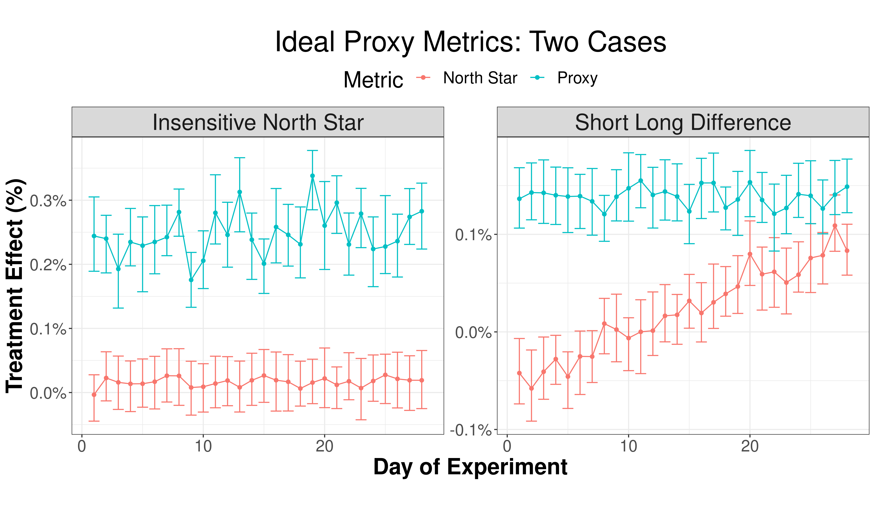
Figure 1: A simulated example of two cases where a proxy metric is useful. The left figure shows the case where the north star metric is positive, but is too small relative to the noise to measure accurately. The right figure shows the case where the north star metric is significantly different in the short and long term, and the proxy metric reflects the long-term impact early in the experiment.

Existing literature on proxy metrics [9, 1] has focused more on predicting the long-term effect, but has not focused on its trade-off with short-term sensitivity. In this paper, we fulfill both goals with a method that optimizes both objectives simultaneously, called Pareto optimal proxy metrics. To our knowledge, this is the first method that explicitly optimizes sensitivity.

The paper is divided as follows. Section 2 discusses how to measure the objectives and their empirical trade-off. Section 3 covers our methodology and algorithms. Section 4 discusses our results, and we conclude in Section 5 with some observations on how to use proxy metrics effectively.

2 How to measure proxy metric performance

The two key properties for metrics are metric sensitivity and directionality [6]. The first refers to the ability of a metric to detect a statistically significant effect, while the second measures the level of agreement between the metric and the long-term effect of the north star. This Section discusses each property individually, and proposes metrics to quantify them. We conclude with our empirical observation regarding the trade-off between sensitivity and directionality, which motivated the methodology in this paper (see Figure 2).

2.1 Metric sensitivity

Metric sensitivity is commonly associated with statistical power. However, it can be expressed as a broader concept [17]. In simple terms, metric sensitivity measures the ability to detect a significant effect for a metric. Following [5], we can write this as

$$P(\text{Reject $H_{0}$})=\int P(\text{Reject $H_{0}$}|\delta)\mathrm{d}P(\delta),$$ (1)

where $\delta$ is the true treatment effect, $P(\text{Reject }H_{0}|\delta)$ is the statistical power, and $\mathrm{d}P(\delta)$ is the distribution of true treatment effects in a population of related experiments. Sensitivity depends heavily on the type of experiments. This is captured in the $\mathrm{d}P(\delta)$ term in Equation 1, and is sometimes referred to as the moveability of the metric. For example, metrics related to Search quality will be more sensitive in Search experiments, and less sensitive in experiments from other product areas (notifications, home feed recommendations, etc.). Although each experiment is unique, our analysis groups together experiments with similar treatments, and we assume that the underlying treatment effects are independent and identically distributed draws from a common distribution of treatment effects.

We need to define quantities that summarize how sensitive a metric is. Our intuition is that we can estimate the probability a metric will detect a statistically significant effect by seeing how often such an effect was statistically significant in historical experiments. Suppose that there are $J$ experiments whose outcome is recorded by $M$ metrics. In each experiment, the population is randomly partitioned into $N\approx 100$ equal groups, and within each group, users are independently assigned to a treatment and a control group. We refer to these groups as independent hash buckets [3].

Let $X_{i,j,m}^{Tr}$ and $X_{i,j,m}^{Ct}$ with $m=1,\ldots,M$ and $j=1,\ldots,J$ denote the short-term recorded values for metric $m$ in experiment $j$ in the treatment and in the control group, respectively, and let $X_{i,j,m}=100\%\times(X_{i,j,m}^{Tr}-X_{i,j,m}^{Ct})/X_{i,j,m}^{Ct}$ their percentage differences, in hash bucket $i=1,\ldots,N$. We refer to these metrics as auxiliary metrics, since their combination will be used to construct a proxy metric in Section 3. The within hash bucket sample sizes are typically large enough that we can use the central limit theorem to assume that $X_{i,j,m}\stackrel{{\scriptstyle\text{iid}}}{{\sim}}N(\theta_{j,m},\sigma^{2}_{j,m})$ for $i=1,\ldots,N$, where $\theta_{j,m}$ and $\sigma^{2}_{j,m}$ are unknown mean and variance parameters, and test

$$H_{0,j,m}:\theta_{j,m}=0\quad\text{vs}\quad H_{1,j,m}:\theta_{j,m}\neq 0.$$

Calling $\bar{X}_{j,m}=N^{-1}\sum_{i=1}^{N}X_{i,j,m}$ the mean percentage difference between the two groups and $se_{j,m}$ the standard error, calculated at Google via the Jackknife method [3], the null hypothesis $H_{0,j,m}$ is rejected at the $\alpha$ level if the test statistics $t_{j,m}=\bar{X}_{j,m}/se_{j,m}$ is larger than a threshold $\tau_{\alpha,N-1}$ in absolute value. The common practice is to let $\alpha=0.05$.

From the above, it naturally follows that metric sensitivity should be directly related to the value of the test statistic $t_{j,m}$. For instance, we call binary sensitivity for metric $m$ the quantity

$$\texttt{BS}(\bar{X}_{\cdot,m})=\frac{1}{J}\sum_{j=1}^{J}\mathds{1}(|t_{j,m}|>\tau_{\alpha,N-1}),\quad(m=1,\ldots,M),$$ (2)

where $\bar{X}_{\cdot,m}=\{\bar{X}_{1,m},\ldots,\bar{X}_{J,m}\}$. Equation (2) measures the proportion of statistically significant experiments in our pool of experiments for every metric $m$. Another characteristic of equation (2) is that it takes on a discrete set of values. This is an issue when the number of experiments $J$ is low. In this case, one can resort to smoother versions of binary sensitivity, such as the average sensitivity, defined as

$$\texttt{AS}(\bar{X}_{\cdot,m})=\frac{1}{J}\sum_{j=1}^{J}|t_{j,m}|,\quad(m=1,\ldots,M).$$ (3)

The above quantity is the average absolute value of the test statistic across experiments. It has the advantage of being continuous and thus easier to optimize, but it pays a cost in terms of lack of interpretability and is also more susceptible to outliers. In the case of large outliers, one effective strategy is to cap the value of the t-statistic.

Which measure of sensitivity to use depends on the application. When a large pool of experiments is available, we recommend using equation (2) due to its interpretation and intrinsic simplicity. Equation (3) should be invoked when optimizing over a discrete quantity yields unstable results.

2.2 Directionality

The second key metric property we need to quantify is called directionality. Through directionality, we want to capture the alignment between the increase (decrease) in the metric and long-term improvement (deterioration) of the user experience. While this is ideal, getting ground truth data for directionality can be complex. A few existing approaches either involve running degradation experiments or manually labeling experiments, as discussed in [6, 7]. Both approaches are reasonable, but suffer from scalability issues.

Our method measures directionality by comparing the short-term value of a metric against the long-term value of the north star. The advantage of this approach is that we can compute the measure in every experiment. The disadvantage is that the estimate of the treatment effect of the north star metric is noisy, which makes it harder to separate the correlation in noise from the correlation in the treatment effects. This can be handled, however, by measuring correlation across repeated experiments.

There are various ways to quantify the directionality of a metric. In this paper, we consider two measures: the first is the mean squared error, while the second is the empirical correlation. Following the setting of Section 2.1, let $Y_{i,j}^{Tr}$ and $Y_{i,j}^{Ct}$ define the long-term value of the north star in the treatment and in the control group for every cookie bucket $i$ and experiment $j$. The resulting recorded percentage difference is $Y_{i,j}=100\%(Y_{i,j}^{Tr}-Y_{i,j}^{Ct})/Y_{i,j}^{Ct}$. Then we can define the mean squared error as

$$\texttt{MSE}(\bar{X}_{\cdot,m})=\frac{1}{J}\sum_{j=1}^{J}(\bar{Y}_{j}-\bar{X}_{j,m})^{2},\quad(m=1,\ldots,M),$$ (4)

where again $\bar{Y}_{j}=N^{-1}\sum_{i=1}^{N}Y_{i,j}$ is the long-term mean of the north star in experiment $j$. Equation (4) measures how well metric $m$ predicts the long-term north star on average. Such a measure depends on the scale of $X$ and $Y$ and may require standardization of the metrics. For a scale-free measure, one instead may adopt correlation, which is defined as follows

$$\texttt{Cor}(\bar{X}_{\cdot,m})=\frac{\sum_{j=1}^{J}(\bar{Y}_{j}-\bar{Y})(\bar{X}_{j,m}-\bar{X})}{\sqrt{\sum_{j=1}^{J}(\bar{Y}_{j}-\bar{Y_{m}})^{2}\sum_{j=1}^{J}(\bar{X}_{j,m}-\bar{X}_{m})^{2}}},\quad(m=1,\ldots,M),$$ (5)

where $\bar{X}_{m}=J^{-1}\sum_{j=1}^{J}\bar{X}_{j,m}$ and $\bar{Y}=J^{-1}\sum_{j=1}^{J}\bar{Y}_{j}$ are the grand mean of metric $m$ and the north star across all experiments.

Equations (4) and (5) quantify the agreeableness between a metric $m$ and the north star, and their use is entirely dependent on the application. Notice that equation (5) measures the linear relationship, but other measures of correlation may be employed, such as Spearman correlation. It is possible to use different measures of correlation because our methodology is agnostic to specific measures of sensitivity and directionality, as detailed in Section 3.

2.3 The trade-off between sensitivity and directionality

So far, we have established two key properties for a metric: sensitivity and directionality. Empirically, we observe an inverse relationship between these two properties. This can be clearly seen from Figure 2, where we plot the value of the binary sensitivity in equation (2) and the correlation with the north star in equation (5) for over 300 experiments on a large industrial recommendation system.

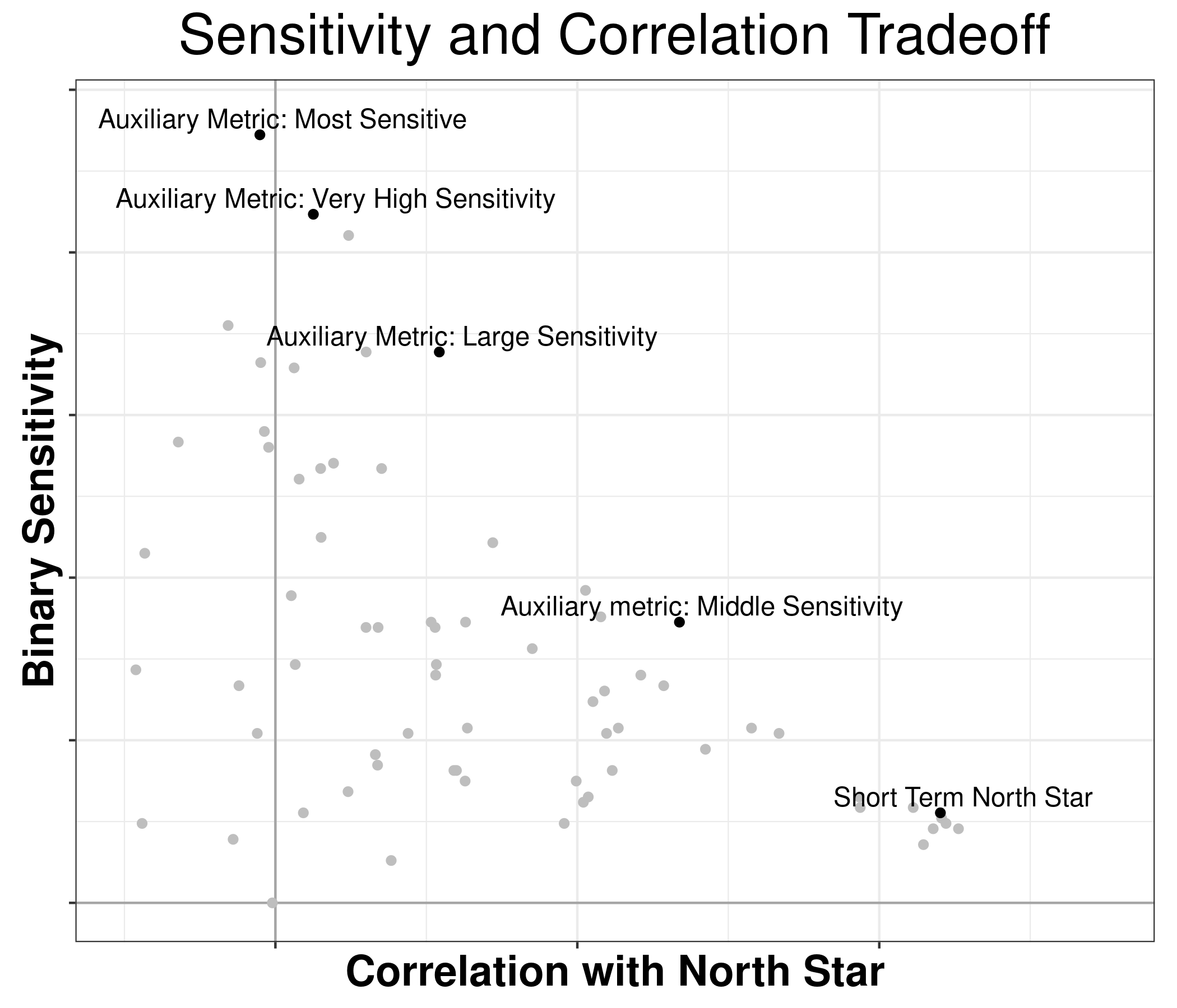
Figure 2: The relationship between correlation and sensitivity for 70 auxiliary metrics across over 300 experiments. Each metric is either a gray or black dot. We highlight several auxiliary metrics that trade-off between sensitivity and correlation in black. Notably, the short-term value of the north star is in the bottom right, which is the least sensitive metric, but the most correlated with the long-term impact of the north star.

As such, there is a trade-off between sensitivity and directionality: the more we increase sensitivity, the less likely our metric will be related to the north star. Thus, our methodology aims to combine auxiliary metrics into a single proxy metric to balance such trade-off in an optimal manner.

3 Pareto optimal proxy metrics

Our core idea is to use multi-objective optimization to learn the optimal trade-off between sensitivity and directionality. Our algorithm learns a set of proxy metrics with the optimal trade-off, known as the Pareto front. The proxy metrics in the Pareto front are linear combinations of auxiliary metrics. Each proxy in the Pareto front is Pareto optimal, in that we can not increase sensitivity without decreasing correlation, and vice versa.

In this section, we first describe the proxy metric problem, and we later cast the proxy metric problem into the Pareto optimal framework. Then we discuss algorithms to learn the Pareto front and compare their performance.

3.1 The proxy metric problem

We define a proxy metric as a linear combination between the auxiliary metrics $m=1,\ldots,M$. Let $\boldsymbol{\omega}=(\omega_{1},\ldots,\omega_{M})$ be a vector of weights. A proxy metric is obtained as

$$Z_{i,j}(\boldsymbol{\omega})=\sum_{m=1}^{M}\omega_{m}X_{i,j,m},$$ (6)

for each $i=1,\ldots,N$ and each experiment $j=1,\ldots,J$. Here, $\omega_{m}$ defines the weight that metric $m$ has on the proxy $Z_{i,j}$. For interpretability reasons, it is useful to consider a normalized version of the weights, namely imposing that $\sum_{m=1}^{M}\omega_{m}=1$ with each $\omega_{m}\geq 0$. In doing so, we require that a positive outcome is associated with an increase in the auxiliary metrics. This means we must swap the sign of metrics whose decrease has a positive impact. These include, for example, metrics that represent bad user experiences, like abandoning the page or refining a query, and which are negatively correlated with the north star metric. Within such a formulation, the proxy metric becomes a weighted average across single metrics where $\omega_{m}$ measures the importance of metric $m$. Un-normalized versions of the proxy weights can also be considered, depending on the context and the measures over which the optimization is carried over. In general, the binary sensitivity in equation (2) and the correlation in equation (5) are invariant to the scale of $\omega_{m}$, which implies that they remain equal irrespective of whether the weights are normalized or not.

Within such a framework, our goal is to find the weights in equation (6). Let $\bar{Z}_{j}(\boldsymbol{\omega})=J^{-1}\sum_{i=N}^{J}Z_{i,j}$ be the average values for the proxy metric in experiments $j=1,\ldots,J$ and $\bar{Z}_{\cdot}(\boldsymbol{\omega})=\{\bar{Z}_{1}(\boldsymbol{\omega}),\ldots,\bar{Z}_{J}(\boldsymbol{\omega})\}$ their collection. When binary sensitivity and correlation are used as measures for sensitivity and directionality, multi-objective optimization is performed via the following problem

$$\boldsymbol{\omega}^{*}={\arg\max}_{\boldsymbol{\omega}=(\omega_{1},\ldots,\omega_{m})}\{\texttt{BS}(\bar{Z}_{\cdot}(\boldsymbol{\omega})),\texttt{Cor}(\bar{Z}_{\cdot}(\boldsymbol{\omega}))\}.$$ (7)

The solution to the optimization in equation (7) is not available in an explicit analytical form, which means that we need to resort to multi-objective optimization algorithms to find $\boldsymbol{\omega}^{*}$. We discuss these algorithms after first introducing the concept of Pareto optimality.

3.2 Pareto optimality for proxy metrics

A Pareto equilibrium is a situation where any action taken by an individual toward optimizing one outcome will automatically lead to a loss in other outcomes. In this situation, there is no way to improve both outcomes simultaneously. If there was, then the current state is said to be Pareto dominated. In the context of our application, the natural trade-off between correlation and sensitivity implies that we cannot unilaterally maximize one dimension without incurring in a loss in the other. Thus, our goal is to look for weights that are not dominated in any dimension. In reference with equation (7), we say that the set of weights $\boldsymbol{\omega}$ is Pareto dominated if there exists another set of weight $\boldsymbol{\omega}^{\prime}$ such that $\texttt{BS}(\bar{Z}_{\cdot}(\boldsymbol{\omega}^{\prime}))\geq\texttt{BS}(\bar{Z}_{\cdot}(\boldsymbol{\omega}))$ and $\texttt{Cor}(\bar{Z}_{\cdot}(\boldsymbol{\omega}^{\prime}))\geq\texttt{Cor}(\bar{Z}_{\cdot}(\boldsymbol{\omega}))$ at the same time. We write $\boldsymbol{\omega}\prec\boldsymbol{\omega}^{\prime}$ to indicate the dominance relationship. Then, the set of non-dominated points is called Pareto set. We indicate it as $\mathcal{W}=\{\boldsymbol{\omega}_{1},\ldots,\boldsymbol{\omega}_{q}\}$, where for all $\boldsymbol{\omega},\boldsymbol{\omega}^{\prime}\in\mathcal{W}$ neither $\boldsymbol{\omega}\prec\boldsymbol{\omega}^{\prime}$ not $\boldsymbol{\omega}^{\prime}\prec\boldsymbol{\omega}$. The objective values associated with the Pareto set are called the Pareto front.

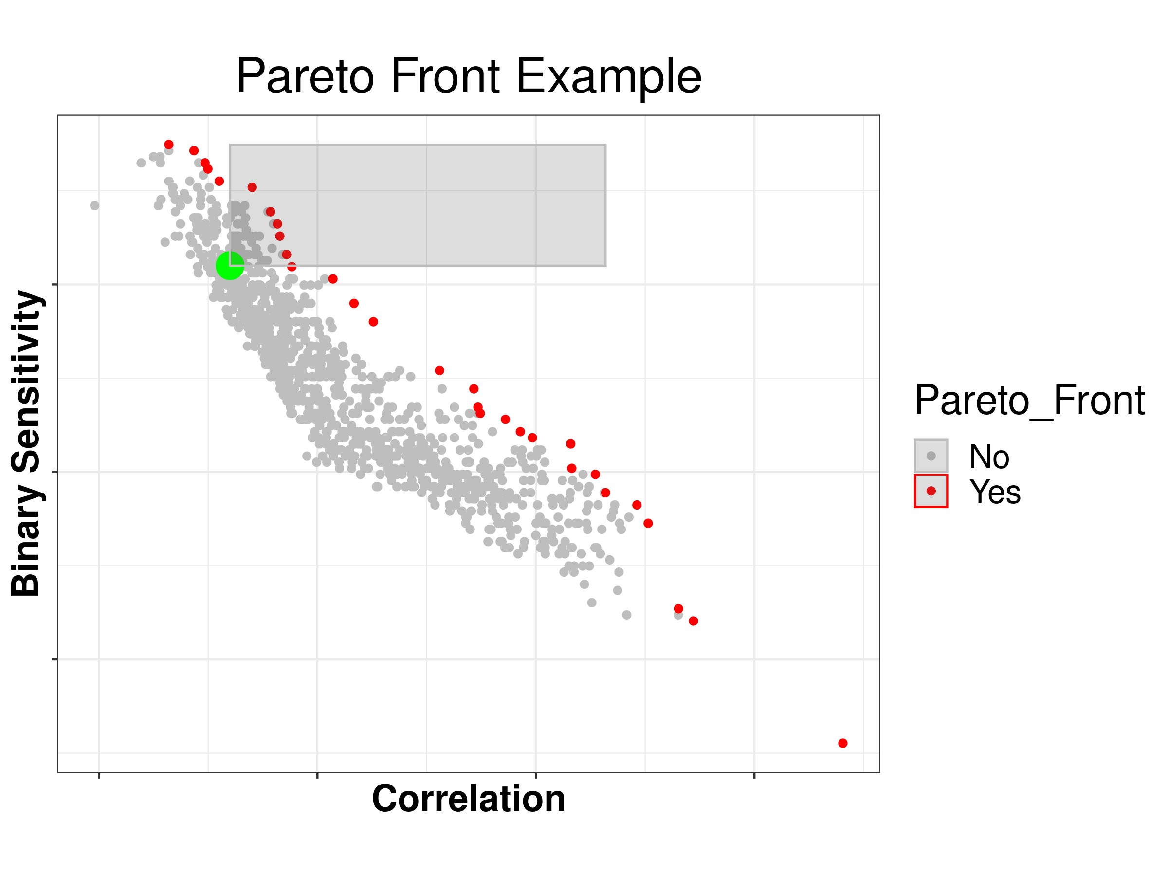
Figure 3: An example of the Pareto front in the proxy metric problem. Each gray dot represents evaluations of the objective in a randomized search. The red dots are points on the Pareto front. The green dot is a point that is Pareto dominated, and the gray shaded area shows where the green dot is Pareto dominated.

Figure 3 shows an example of what the Pareto front and the Pareto set look like. The grey points represent the value of the objectives for a set of weights generated at random, while the red points are the ones in the Pareto set. The green dot is an example point that is Pareto dominated by the area highlighted in grey. It is easy to see that any point in the grey area is strictly better than the green dot. The purpose of multi-objective optimization is to efficiently identify the Pareto front and the weights in the Pareto set. Algorithms to estimate the Pareto front are reported in the next Section.

3.3 Algorithms for Pareto optimal proxies

Multi-objective optimization is a well-studied problem that can be solved via a wealth of efficient algorithms. Common methods to extract the Pareto front combine Kriging techniques with expected improvement minimization [11, 20], or black box methods via transfer learning [19, 13]. These methods are particularly suitable for cases where the objective functions are intrinsically expensive to calculate, and therefore one wishes to limit the number of evaluations required to extract the front. In our case, however, both objective functions can be calculated with minimal computational effort. As such, we propose two algorithms to efficiently extract the front that rely on sampling strategies and nonlinear optimization routines. We then compare our algorithms against a standard Kriging-based implementation.

Our first method to extract the Pareto front involves a simple randomized search, as described in Algorithm 1 below. The mechanism is relatively straightforward: at each step, we propose a candidate weight $\boldsymbol{\omega}$ and calculate the associated proxy $Z_{i,j}$ for every $i=1,\ldots,N$ and every experiment $j=1,\ldots,J$. Then, we evaluate the desired objective functions, such as the binary sensitivity and the correlation in equations (2) and (5). These allow us to tell whether $\boldsymbol{\omega}$ is dominated. In the second case, we update the Pareto front by removing the Pareto dominated weights and then by including the new one in the Pareto set.

Algorithm 1 Randomized search

1:Input: Number of samples $T$, single metrics $X$, north start $Y$

2:Output: Pareto set $\mathcal{W}$

3:Initialize the Pareto set to be empty: $\mathcal{W}=\emptyset$.

4:for $t=1\ldots,T$ do

5:     Sample $\boldsymbol{\omega}=\{\omega_{1},\ldots,\omega_{M}\}$ uniformly in $[0,1]$.

6:     Calculate $Z_{i,j}(\boldsymbol{\omega})$ as in equation (6).

7:     Evaluate $\texttt{BS}(\bar{Z}_{\cdot}(\boldsymbol{\omega}))$ and $\texttt{Cor}(\bar{Z}_{\cdot}(\boldsymbol{\omega}))$ (or any other objective function).

8:     If $\boldsymbol{\omega}$ is not dominated by any other $\boldsymbol{\omega}^{\prime}\in\mathcal{W}$, add $\boldsymbol{\omega}$ to $\mathcal{W}$.

9:     Remove the weights in $\mathcal{W}$ that are dominated.

10:end for

The advantage of Algorithm 1 is that it explores the whole space of possible weights and can be performed online with minimum storage requirements. However, such exploration is often inefficient, since the vast majority of sampled weights are not on the Pareto front. Moreover, the method may suffer from a curse of dimensionality: if the total number of auxiliary metrics $M$ is large, then a massive number of candidate weights is required to explore the hypercube $[0,1]^{M}$ exhaustively. A standard solution to such a problem relies on a more directed exploration of the space of weights via Kriging, where the weight at one iteration is sampled from normal distributions whose mean and variance are obtained by minimizing an in-fill criterion [11]. Refer to [2] for a practical overview. Since evaluating sensitivity and correlation is a relatively simple operation, we propose a more directed algorithm, which we now illustrate.

Consider the bivariate optimization problem in equation (7). If we fix one dimension, say sensitivity, to a certain threshold and later optimize with respect to the other dimension in a constrained manner, then varying the threshold between 0 and 1 should equivalently extract the front. In practice, this procedure is approximated by binning the sensitivity in disjoint intervals, say $[u_{b},u_{b+1})$ with $b=1,\ldots,B-1$, with $u_{1}=0$ and $u_{B}=1$, and then solving

$$\begin{split}\boldsymbol{\omega}^{*}_{b}={\arg\max}_{\boldsymbol{\omega}:\ \texttt{BS}(\bar{Z}_{\cdot}(\boldsymbol{\omega}))\in[u_{b},u_{b+1})}\ \texttt{Cor}(\bar{Z}_{\cdot}(\boldsymbol{\omega})),\end{split}$$ (8)

for each $b=1,\ldots,B-1$. The resulting Pareto front is composed of a length $B$ set of weights. We summarize this in Algorithm 2 below.

Algorithm 2 Constrained optimization via binning

1:Input: Number of samples $T$, single metrics $X$, north start $Y$, sensitivity bins $[u_{b},u_{b+1})$

2:Output: Pareto set $\mathcal{W}$ (approximation)

3:Initialize the Pareto set to be empty: $\mathcal{W}=\emptyset$.

4:for $b=1\ldots,B-1$ do

5:     Solve the constrained optimization in equation (8) via nlopt.

6:     Add $\boldsymbol{\omega}_{b}$ to $\mathcal{W}$

7:end for

The optimization problem in equation (7) and Algorithm 2 can be solved via common nonlinear optimization methods such as the ones in the nlopt package. See [15] and references therein.

Each algorithm produces a set of Pareto optimal proxy metrics. However, we typically rely on a single proxy metric for experiment evaluation and launch decisions. This means we need to select a proxy from the Pareto front. In practice, we use the Pareto set to reduce the space of candidate proxies, and later choose the final weights based on statistical properties and other product considerations.

3.4 Algorithm performance

This Section evaluates the performance of our proposed algorithms. The task is extracting the Pareto front between binary sensitivity and correlation from a set of over 300 experiments. Details on the data are described in Section 4. We test three different algorithms:

1. Randomized search (Algorithm 1). We let the algorithm run for $M\times 4000$ iterations.

2. Constrained optimization via binning (Algorithm 2). We split sensitivity into 14 discrete bins, ranging from $0$ to the maximum sensitivity of a single metric in our data set. From the nlopt package, we rely on the locally biased dividing rectangles algorithm [12].

3. Kriging and minimization of the expected increase in hyper-volume [11], using the R package GPareto [2]. We let the algorithm run for $M\times 40$ iterations.

We estimate the Pareto front for $M=5,10,\text{ and }15$ metrics to understand how algorithm performance scales in the number of metrics. Figure 4 compares the Pareto front extracted by each algorithm. Each algorithm yields a similar Pareto front. We notice that constrained optimization detects points in high sensitivity and high correlation regions better than the other two methods, especially as the number of metrics increases. However, the middle of these extracted curves are very similar.

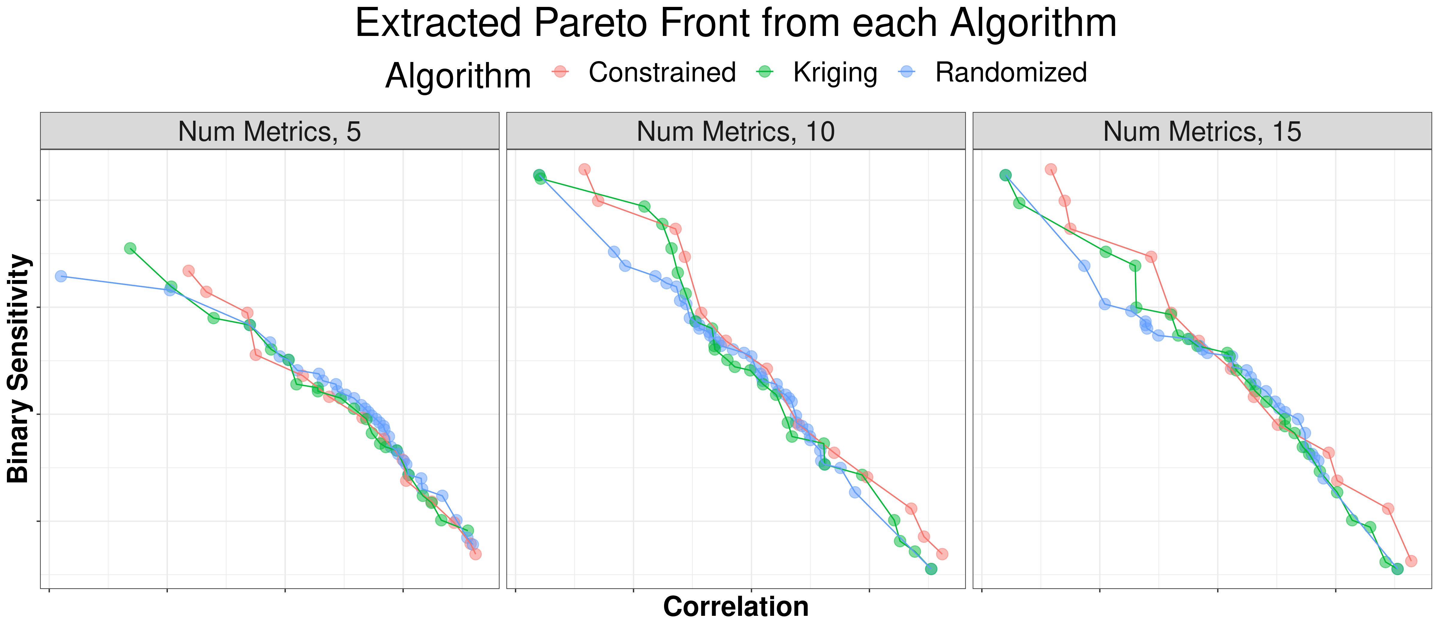
Figure 4: Pareto front extracted under the three methods.

A more direct comparison is reported in Figure 5. Here, we quantify the extracted Pareto Front using the Area under the Pareto Front metric (larger values are better). We also compare the run-time of each algorithm. The clear takeaway from Figure 5 is that the choice of algorithms does not matter much for a small number of metrics (5). However, constrained optimization is the best trade-off between accuracy and speed when the number of metrics is large.

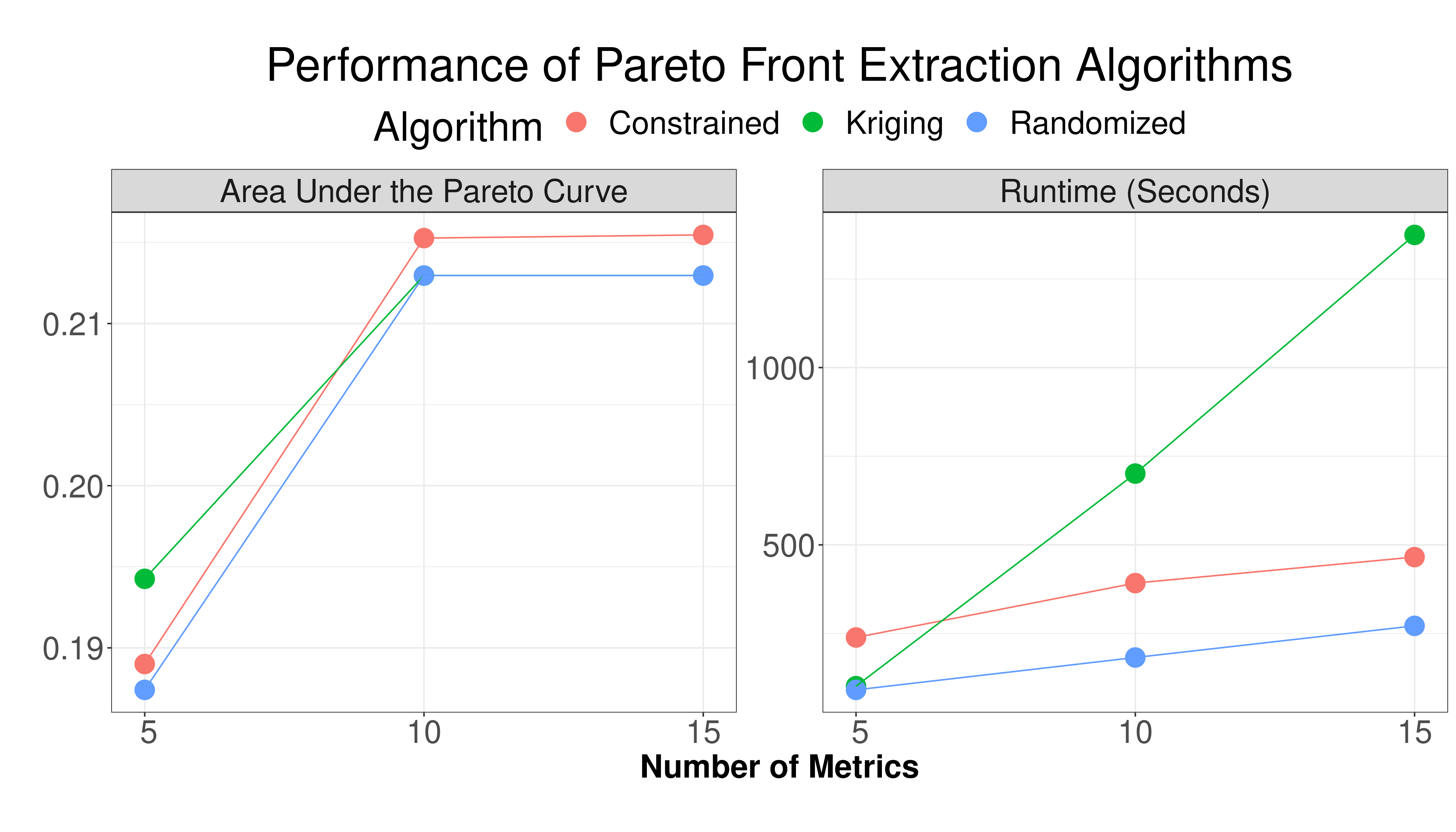
Figure 5: The left plot shows the Area under the Pareto curve for each algorithm, the right plot shows how long each algorithm took to extract the Pareto front in Figure 4

4 Results

We implemented our methodology on over 300 experiments in a large industrial recommendation system. We then evaluated the performance of the resulting proxy on over 500 related experiments that ran throughout the subsequent six months. Specifically, we compare the proxy with the short-term north star metric, since its precise goal is to improve upon the sensitivity of the short-term north star itself. As success criteria, we use Binary Sensitivity in equation (2) and the proxy score, which is a one-number statistic that evaluates proxy quality. See Appendix A for a detailed definition.

Table 1 compares our short-term proxy metric against the short-term north star metric. Our proxy metric was 8.5 times more sensitive. In the cases where the long-term north star metric was statistically significant, the proxy was statistically significant 72% of the time, compared to just 40% of the time for the short-term north star. In this set of experiments, we did not observe any case where the proxy metric was statistically significant in the opposite direction as the long-term north star metric. We have, however, seen this occur in different analyses. But the occurrence is rare and happens in less than 1% of experiments. Finally, our proxy metric has a 50% higher proxy score than the short-term north star. Our key takeaway is that we can find proxy metrics that are dramatically more sensitive while barely sacrificing directionality.

Table 1: Comparison of using the short-term north star metric and the Pareto optimal proxy metric. This table was constructed on a set of experiments that ran for six months after we implemented our proxy. The sensitivity of our proxy is 8.5X%, compared to just X% for the north star.

	short term north star	proxy
Proxy Score	0.41	0.72
Binary Sensitivity	X%	8.5X%
Recall	0.41	0.72
Precision	1.0	1.0

Table 1 only evaluates the relationship between the proxy and north star metric when the north star is statistically significant. These experiments are useful because we have a clear direction from the north star metric. However, it is also important to assess the proxy metric when the long-term north star metric is neutral. For this, we can look at the magnitude of the north star metric when the long-term effect is not statistically significant, split by whether the proxy is negative, neutral, or positive. We display this in Figure 6, which shows that, although we may not get statistically significant results for the north star metric, making decisions based on the proxy will be positive for the north star on average. In practice, we are careful when rolling out these cases, and have tools to catch any launch that does not behave as expected.

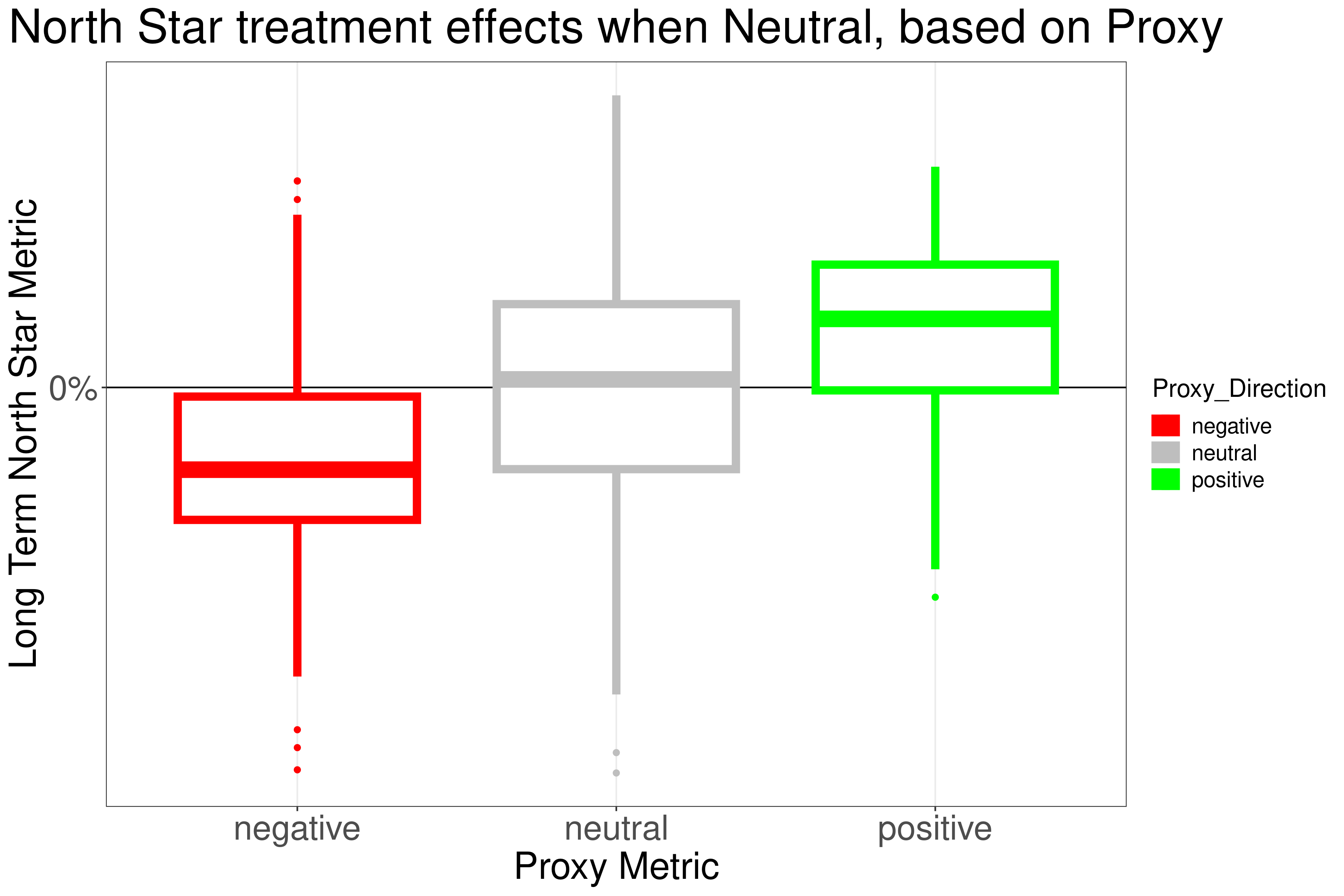
Figure 6: The magnitude of the long-term north star treatment effect, when the long-term treatment effect is neutral, depending on if the proxy metric is negative, neutral, or positive.

Finally, it is instructive to analyze how the weights of the proxy metrics vary as we move along the Pareto front from directionality to sensitivity, as illustrated in the example in Figure 7. As expected, when we select points that emphasize correlation, our proxy metric puts more weight on the short-term north star. But when we choose points that emphasize sensitivity, we put much more weight on sensitive, local metrics.

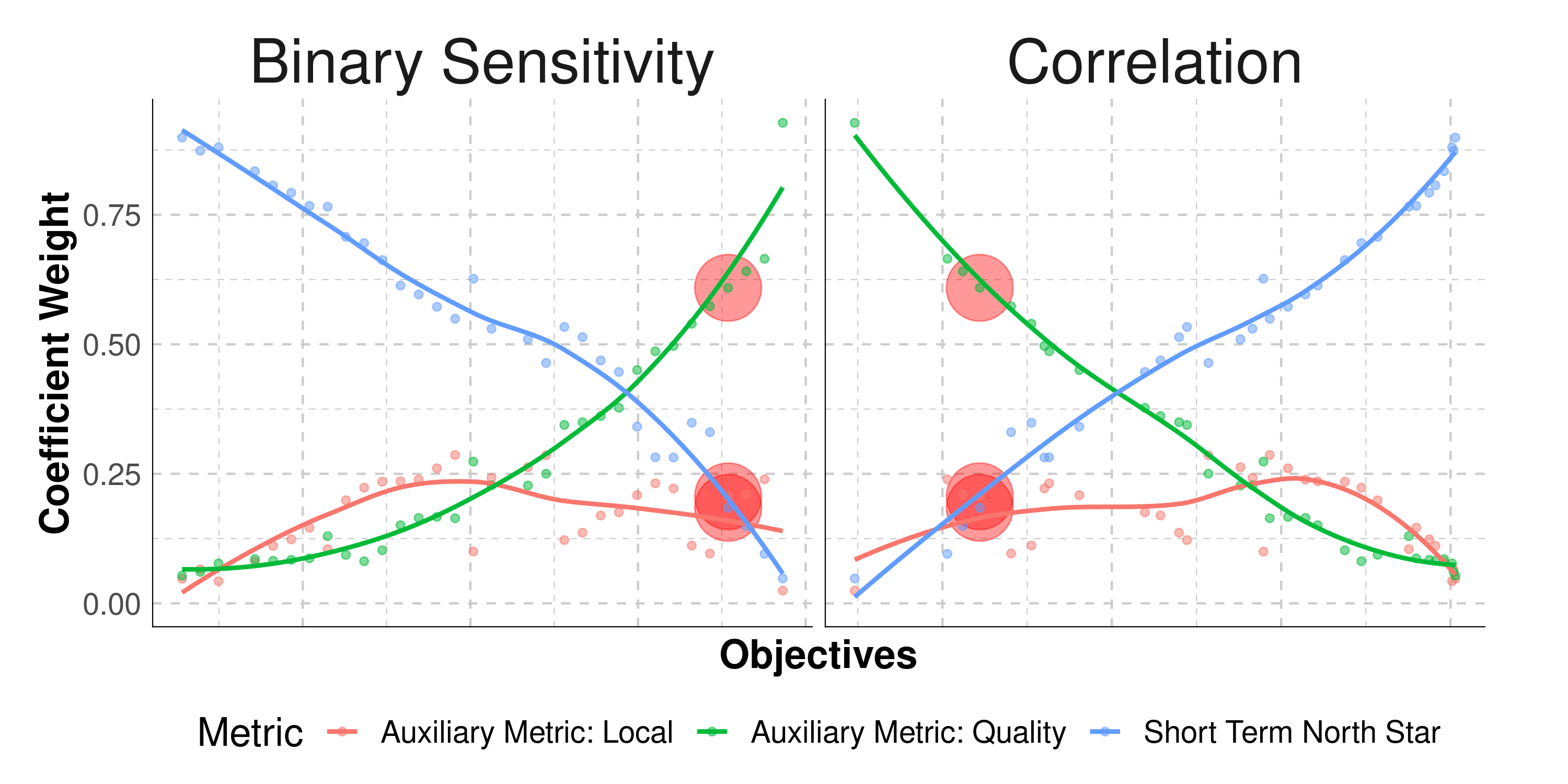
Figure 7: Weights of the proxy metrics in the Pareto set as a function of both objectives. We include three metrics, the short-term north star and two metrics that are more sensitive, capturing different elements of the user experience. The optimal weights are highlighted in red for both objectives. In this example, we choose the point that optimized the Area under the Pareto Curve.

5 Discussion

This paper proposes a new method to find proxy metrics that optimizes the trade-off between sensitivity and directionality. To our knowledge, this is the first approach that explicitly incorporates metric sensitivity into the objective. In our experiments, we found proxy metrics that were 6-10 times more sensitive than the short-term north star metric, and minimal cases where the proxy and the north star moved in opposite directions.

Our experience developing proxy metrics with multiple teams across multiple years has spurred many thoughts on their pros, cons, and things to watch out for. These considerations go beyond the mathematical framework discussed in this paper, and we list them in the next section. We then discuss some other benefits of using proxy metrics. Finally, we’ll discuss some limitations in our methodology and future areas of improvement.

5.1 Considerations beyond Pareto optimality

Below are other important considerations we learned from deploying proxy metrics in practice:

• Make sure you need proxies before developing them. Proxies should be motivated by an insensitive north star metric, or one that is consistently different between the short and long term. It is important to validate that you have these issues before developing proxies. To assess sensitivity, you can compute the Binary Sensitivity in a set of experiments. To assess short and long-term differences, one possibility is to compare the treatment effects at the beginning and end of your experiments.

• Try better experiment design before using proxies. Proxies are one way to increase sensitivity, but they are not the only way. Before you create proxy metrics, you should assess if your sensitivity problems can be solved with a better experiment design. For example, you may be able to run larger experiments, longer experiments, or narrower triggering to only include users that were actually impacted by the treatment. Solving at the design stage is ideal because it allows us to target the north star directly.

• Choose proxies with common sense. The best auxiliary metrics in our proxy metric captured intuitive, critical aspects of the specific user journey targeted by that class of experiments. For example, whether a user had a satisfactory watch from the homepage is a good auxiliary metric for experiments changing the recommendations on the home feed. In fact, many of the best auxiliary metrics were already informally used by engineers, suggesting that common sense metrics have superior statistical properties.

• Validate and monitor your proxies, ideally using holdbacks. It is important to remember that proxy metrics are not what we want to move. We want to move the north star, and proxies are a means to this end. The best tool we have found for validating proxies is the cumulative long-term holdback, including all launches that were made based on the same proxy metric. It is also helpful to regularly repeat the model fitting process on recent data, and perform out-of-sample testing, to ensure your proxy is still at an optimal point.

5.2 Other benefits of proxy metrics

Developing proxies had many unplanned benefits beyond their strict application as a tool for experiment evaluation. The first major benefit is the sheer educational factor: the data science team and our organizational partners developed a much deeper intuition about our metrics. We learned baseline sensitivities, how the baseline sensitives vary across different product areas, and the correlations between metrics.

Another unplanned benefit is that the proxy metric development process highlighted several areas to improve the way we run experiments. We started to do better experiment design, and to collect data from experiments more systematically, now that the experiments can also be viewed as training data for proxy metrics.

Finally, the most important benefit is that we uncovered several auxiliary metrics that were correlated with the north star, but not holistic enough to be included in the final proxy. We added these signals directly into our machine-learning systems, which resulted in several launches that directly improved the long-term user experience.

5.3 Discussion, limitations, and future directions

This methodology is an important milestone, but there are still many areas to develop, and our methodology is sure to evolve over time.

The first area to explore is causality. Our approach relies on the assumption that the treatment effects of the experiments are independent draws from a common distribution of treatment effects, and that future experiments come from the same generative process. Literature from clinical trials [16, 10], however, has more formal notions of causality for surrogate metrics, and we plan to explore this area and see if there’s anything we can glean.

Another important improvement would be a more principled approach to select the final proxy metric. Some initial work along these lines revolves around our proxy score (Appendix A) and Area under the Pareto curve (Figure 4). We hope to have a more refined perspective on this topic in the future.

We also did not explore more classic model-building improvements in detail. For example, we do not address non-linearity and feature selection. Non-linearity is particularly important, because it helps in cases where two components of the proxy metric move in opposite directions. For feature selection, we currently hand-pick several auxiliary metrics to include in the proxy metric optimization. However, we should be able to improve upon this by either inducing sparsity when estimating the Pareto front, or adopting a more principled feature selection approach.

To conclude, let’s take a step back and consider the practical implications of our results. Essentially, we found that the appropriate local metrics, that are close to the experiment context, are vastly more sensitive than the north star, and rarely move in the opposite direction. The implication is that using the north star as a launch criterion is likely too conservative, and teams can learn more and faster by focusing on the relevant local metrics.

Faster iteration has also opened our eyes to other mechanisms we can use to ensure that our launches are positive for the user experience. We mentioned earlier that launches using proxies should be paired with larger and longer running holdbacks. In fact, through such holdbacks we were able to catch small but slightly negative launches (case 1 in Figure 1, but with the opposite sign), and further refine our understanding of the differences between the short and long term impact on the north star metric (case 2 in Figure 1, but with the opposite sign).

Appendix A The proxy score

It is useful to have a single metric that quantifies the performance of a proxy metric. We have relied on a measure called proxy score. The proxy score rewards properties of an ideal proxy metric: short-term sensitivity, and moving in the same long-term direction as the north star (Figure 1). The motivation behind our specific definition comes from the contingency table visualized in Figure 8, which is generated from 1000 simulated experiments.

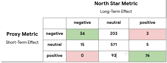
Figure 8: There are nine combinations of statistical significance between the proxy metric and the north star metric, based on if the proxy and north star are negative, neutral, or positive.

The green cells in Figure 8 represent cases where the proxy is statistically significant in the short-term, the north star is significant in the long-term, and the proxy and north star move in the same direction. These are unambiguously good cases, and we refer to them as Detections. The red cells are unambiguously bad cases: both the short-term proxy and north star are statistically significant, but they move in opposite directions. We call these Mistakes. Informally, we define the proxy score as

Proxy Score $$= \frac{\text{Detections}-\text{Mistakes}}{\text{Number of experiments where the north star is significant}}.$$

The key idea is that the proxy score rewards both sensitivity, and accurate directionality. More sensitive metrics are more likely to be in the first and third rows, where they can accumulate reward. But metrics in the first and third rows can only accumulate reward if they are in the correct direction. Thus, the proxy score rewards both sensitivity and directionality. Microsoft independently developed a similar score, called Label Agreement [7].

More formally, and following the notation in Section 2, we can define the proxy score using hypothesis tests for the proxy metric and the north star metric, defined as

North Star: $$\qquad H_{0,j}^{ns}:\theta_{j}^{ns}=0\quad\text{vs}\quad H_{1,j}^{ns}:\theta^{ns}_{j}\neq 0,$$ (9)

Proxy: $$\qquad H_{0,j}^{z}:\theta_{j}^{z}=0\quad\text{vs}\quad H_{1,j}^{z}:\theta^{z}_{j}\neq 0.$$ (10)

If we let $D_{j}=\{\theta_{j}^{ns},\sigma_{j}^{ns},\theta_{j}^{z},\theta_{j}^{z}\}$ be data required to compute the hypothesis tests, then the proxy score for experiment $j$ can be written as

$$\texttt{PS}(D_{j}) = \mathbf{1}(H^{z}_{0,j}\text{ rejected})\qquad(\text{Proxy Significant})$$

$$\times \mathbf{1}(H^{ns}_{0,j}\text{ rejected})\qquad(\text{North Star Significant})$$

$$\times \Big{[}\mathbf{1}(\theta_{j}^{ns}>0\text{ and }\theta_{j}^{z}>0)+\mathbf{1}(\theta_{j}^{ns}<0\text{ and }\theta_{j}^{z}<0)\Big{]}\quad(\text{Agree})$$

$$\times \Big{[}-\mathbf{1}(\theta_{j}^{ns}>0\text{ and }\theta_{j}^{z}<0)-\mathbf{1}(\theta_{j}^{ns}<0\text{ and }\theta_{j}^{z}>0)\Big{]},\ \ (\text{Disagree})$$

where $\mathbf{1}(\cdot)$ is an indicator equal to one if its argument is true, and zero otherwise.

We can aggregate these values across all experiments in our data, and scale by the number of experiments where the north star is significant, to compute the final proxy score for a set of experiments. The scaling factor ensures that the proxy score is always between -1 and 1.

$$\texttt{PS}(D) = \sum_{j=1}^{J}\frac{\texttt{PS}(D_{j})}{\mathbf{1}(H^{ns}_{0,j}\text{ rejected})}.$$ (11)

Similar to Binary sensitivity, there can be issues with the proxy score when the north star metric is rarely significant. We have explored a few ways to make this continuous, for example by substituting indicators for Bayesian posterior probabilities.

References

- [1] Susan Athey, Raj Chetty, Guido W Imbens, and Hyunseung Kang. The surrogate index: Combining short-term proxies to estimate long-term treatment effects more rapidly and precisely. Technical report, National Bureau of Economic Research, 2019.
- [2] Mickaël Binois and Victor Picheny. GPareto: An R package for gaussian-process-based multi-objective optimization and analysis. Journal of Statistical Software, 89(8):1–30, 2019.
- [3] Nicholas Chamandy, Omkar Muralidharan, Amir Najmi, and Siddartha Naidu. Estimating uncertainty for massive data streams. Technical report, Google, 2012.
- [4] Albert C. Chen and Xin Fu. Data + intuition: A hybrid approach to developing product north star metrics. In Proceedings of the 26th International Conference on World Wide Web Companion, WWW ’17 Companion, page 617–625, Republic and Canton of Geneva, CHE, 2017. International World Wide Web Conferences Steering Committee.
- [5] Alex Deng. Metric Sensitivity Decomposition. Causal Inference and Its Applications in Online Industry. https://alexdeng.github.io/causal/sensitivity.html#metric-sensitivity-decomposition. [Online; accessed 21-December-2022].
- [6] Alex Deng and Xiaolin Shi. Data-driven metric development for online controlled experiments: Seven lessons learned. In Proceedings of the 22nd ACM SIGKDD International Conference on Knowledge Discovery and Data Mining, pages 77–86, 2016.
- [7] Pavel Dmitriev and Xian Wu. Measuring metrics. In Proceedings of the 25th ACM international on conference on information and knowledge management, pages 429–437, 2016.
- [8] Weitao Duan, Shan Ba, and Chunzhe Zhang. Online experimentation with surrogate metrics: Guidelines and a case study. In Proceedings of the 14th ACM International Conference on Web Search and Data Mining. ACM, mar 2021.
- [9] Weitao Duan, Shan Ba, and Chunzhe Zhang. Online experimentation with surrogate metrics: Guidelines and a case study. In Proceedings of the 14th ACM International Conference on Web Search and Data Mining, pages 193–201, 2021.
- [10] Michael R Elliott, Anna SC Conlon, Yun Li, Nico Kaciroti, and Jeremy MG Taylor. Surrogacy marker paradox measures in meta-analytic settings. Biostatistics, 16(2):400–412, 2015.
- [11] Michael T. M. Emmerich, André H. Deutz, and Jan Willem Klinkenberg. Hypervolume-based expected improvement: Monotonicity properties and exact computation. In 2011 IEEE Congress of Evolutionary Computation (CEC), pages 2147–2154, 2011.
- [12] Joerg M Gablonsky and Carl Tim Kelley. A locally-biased form of the direct algorithm. Technical report, North Carolina State University. Center for Research in Scientific Computation, 2000.
- [13] Daniel Golovin, Benjamin Solnik, Subhodeep Moitra, Greg Kochanski, John Karro, and D. Sculley. Google vizier: A service for black-box optimization. In Proceedings of the 23rd ACM SIGKDD International Conference on Knowledge Discovery and Data Mining, Halifax, NS, Canada, August 13 - 17, 2017, pages 1487–1495. ACM, 2017.
- [14] Henning Hohnhold, Deirdre O’Brien, and Diane Tang. Focus on the long-term: It’s better for users and business. In Proceedings 21st Conference on Knowledge Discovery and Data Mining, Sydney, Australia, 2015.
- [15] Steven G. Johnson. The NLopt nonlinear-optimization package. https://github.com/stevengj/nlopt, 2007.
- [16] Ross L. Prentice. Surrogate endpoints in clinical trials: definition and operational criteria. Statistics in medicine, 8(4):431–440, 1989.
- [17] W. Qin, W. Machmouchi, and Martins A. M. Beyond power analysis: Metric sensitivity analysis in A/B tests. https://www.microsoft.com/en-us/research/group/experimentation-platform-exp/articles/beyond-power-analysis-metric-sensitivity-in-a-b-tests/.
- [18] Lenny Rachitsky. Choosing Your North Star Metric. https://future.com/north-star-metrics/.
- [19] Xingyou Song, Sagi Perel, Chansoo Lee, Greg Kochanski, and Daniel Golovin. Open source vizier: Distributed infrastructure and api for reliable and flexible black-box optimization. In Automated Machine Learning Conference, Systems Track (AutoML-Conf Systems), 2022.
- [20] Kaifeng Yang, Michael Emmerich, André Deutz, and Thomas Bäck. Multi-objective bayesian global optimization using expected hypervolume improvement gradient. Swarm and Evolutionary Computation, 44:945–956, 2019.