The Prophet Secretary and its Variants via Poissonization and Sharding

Abstract

We introduce a new technique (i.e. sharding) of breaking up random variables into many independent random variables that behaves together as the original single random variable. This in turn enables us to model the random variables using a Poisson distribution (i.e., Poissonization). These two ideas, leads to an improved analysis of the Prophet Secretary problem and its variants. Beyond the (small but significant) improvement in the constants, the new analysis is significantly simpler and more intuitive than previous (quite involved) analysis. We also get several simpler proofs of existing known results. The new approach might be of independent interest to the order-selection variant of the prophet inequality.

1 Introduction, Related Work, and Contributions

The field of optimal stopping theory concerns the optimization settings where one makes decisions in a sequential manner, given imperfect information about the future, with an objective to maximize a reward or minimize a cost. The classical problem in the field is known as the prophet inequality problem [KS77, KS78]. In this problem, a gambler is presented $n$ non-negative independent random variables $X_{1},\ldots X_{n}$ with known distributions in this order. In iteration $t$, a random realization $x_{t}$ is drawn from the distribution of $X_{t}$ and presented to the gambler. The gambler can then choose to either accept $x_{t}$, ending the game, or irrevocably rejecting $x_{t}$ and continuing to iteration $t+1$. Note that the random variable ordering is chosen adversarially by an almighty adversary that knows the gambler’s algorithm. The goal of the gambler is to maximize their expected reward, where the expectation is taken across all possible realizations of $X_{1},\ldots,X_{n}$. The gambler is compared to a prophet who is allowed to make their decision after seeing all realizations (i.e. can always get $\max(x_{1},\ldots x_{n})$) regardless what realizations occur. In other words, the prophet gets a value $P$ with expectation $\mathop{\mathbb{E}}\!\left[{P}\right]=\mathop{\mathbb{E}}\!\left[{\max(X_{1},\ldots X_{n})}\right]$. An algorithm ALG is $\alpha$-competitive, for $\alpha\in[0,1]$, if $\mathop{\mathbb{E}}\!\left[{{\textsf{ALG}}}\right]\geq\alpha\cdot\mathop{\mathbb{E}}\!\left[{P}\right]$, and $\alpha$ is called the competitive ratio.

The prophet inequality problem has a $1/2$-competitive algorithm. The first algorithm to give the $1/2$ analysis is due to Krengel and Sucheston [KS77, KS78]. Later, Samuel-Cahn [SC84] gave a simple algorithm that sets a single threshold $\tau$ as the median of the distribution of $Z=\max_{i}X_{i}$, and accepts the first value (if any) above $\tau$. She showed that the algorithm is $1/2$ competitive and, moreover, this is tight. Kleinberg and Weinberg [KW19] also showed that setting $\tau=\mathop{\mathbb{E}}\!\left[{\max_{i}X_{i}}\right]/2$ also gives a $1/2$-competitive algorithm.

The above discussion makes no assumption on the distributions of $X_{1},\ldots,X_{n}$ excepting independence. If $X_{1},\ldots,X_{n}$ are IID random variables, then Hill and Kertz [HK82] initially gave a $(1-1/e)$-competitive algorithm. This was improved by Abolhassani, Ehsani, Esfandiari, Hajiaghayi, and Kleinberg [AEE⁺17] in STOC 2017 into a $\approx 0.738$ competitive algorithm. Finally, this was improved to $\approx 0.745$ in a result due to Correa, Foncea, Hoeksma, Oosterwijk, and Vredeveld [CFH⁺21]. This constant is tight due to a matching upper bound, and hence the IID special case is also resolved.

Several variations on the prophet inequality problem are known. We list some below.

Problem 1.1.

Random-Order: The variant of the prophet inequality problem where the random variables realizations arrive at a random-order drawn uniformly from $\mathbb{S}_{n}$. This is also known as the prophet secretary problem.

Problem 1.2.

Order-Selection: The variant of the prophet inequality problem where the gambler can choose the order that the random variables are provided.

Problem 1.3.

Semi-Online: Here, the values are not provided, but instead the gambler can issue $n$ queries of the form “ Is $X_{i}\geq\tau_{i}$?” for any desired $\tau_{i}$, which can be chosen adaptively. Each random variable can only be queried once. Finally, after using the $n$ queries, we choose the variable with the maximum conditional expectation.

Problem 1.4.

Semi-Online-Load-Minimization: The same as the semi-online setting, but we are allowed to query a variable multiple times. In particular, we can use at most $n$ queries in total, and the goal is to get a $1-o(1)$ competitive ratio while minimizing the maximum number of queries a variable is asked (i.e. the load).

Problem 1.5.

Best 1-of-$k$: The variant of the prophet inequality problem where the random variables are presented adversarially in the order $X_{1},...,X_{n}$, and the gambler is allowed to choose at most $k\geq 2$ realizations (instead of $1$). Finally, they get the maximum value of the values they have chosen. This is also referred to as prophet inequality with overbooking.

Prophet Secretary

In terms of the random-order problem, Esfandiari, Hajiaghayi, Liaghat, and Monemizadeh [EHLM17] initially gave a $1-\frac{1}{e}\approx 0.632$ competitive algorithm. This was later improved in a surprising result by Azar, Chiplunkar, and Kaplan [ACK18] into a $1-\frac{1}{e}+\frac{1}{400}\approx 0.63{\bf 4}$ competitive algorithm in EC 2018. While the improvement is small, the case-by-case analysis introduced was non-trivial, exposing the intricacies of the problem. In a subsequent elegant result, Correa, Saona, and Ziliotto [CSZ20] improved this to a $0.6{\bf 69}$ competitive algorithm by introducing the notion of discrete blind strategies at SODA 2019. This required less case-by-case analysis. However, it should be noted that this result holds only approximately (i.e. the algorithm converges to $\approx 0.669$ as $n\to+\infty$). Meanwhile, current impossibility results show that no algorithm can achieve a competitive ratio better than $0.7235$ [GMTS23].

Order-selection

The order-selection problem has had more progress than random-order. Specifically, since a random-order is a valid order for order-selection, then the result of Correa et al. [CSZ20] of $\approx 0.669$ remained the state of the art. This was improved recently in FOCS 2022 to a $0.7251$-competitive algorithm by Peng and Tang [PT22]. They showed a separation between random-order and order-selection: recall that no algorithm can do better than $0.7235$ for random-order, and so there is a strict advantage of order-selection over random-order. Thus, the optimal order-selection strategy is not a random permutation. In addition, the methods developed were of interest for similar variations of the problem. In a followup work at EC 2023, Bubna and Chiplunkar [BC23] showed that the analysis of Peng et al. method cannot be improved, and gave an improved $0.725{\bf 8}$ competitive algorithm (i.e. improvement in the $4\textsuperscript{th}$ digit) for order-selection using a different approach. Note, the separation result was established independently by Giambartolomei, Mallmann-Trenn and Saona in [GMTS23] around the same time.

Semi-Online

Hoefer and Schewior [HS23] introduced the semi-online prophet inequalities variants. They only studied the case where the variables are IID (i.e. Semi-Online and Semi-Online-Load-Minimization for IID random variables) and left the more general Non-IID versions for future work. For the IID Semi-Online problem, they give a $0.869$ competitive algorithm, significantly surpassing the $\approx 0.745$ ratio for the classical IID prophet inequality. In addition, they showed no algorithm can do better than $0.9799$. They also showed that Semi-Online-Load-Minimization can be solved for IID random variables with an $O(\log(n))$ load. Nothing is known for the non-IID Semi-Online-Load-Minimization.

Best 1-of-$k$

Assaf and Samuel-Cahn [ASC00] introduced the best 1-of-$k$ variant to the prophet inequality. They gave a simple and elegant $k/(k+1)$ competitive algorithm for all $k\geq 2$. They also showed that for $k=2$, one cannot do better than $0.8$. In a followup paper, Assaf, Samuel-Cahn, and Goldstein [AGSC02] gave a significantly tighter analysis on $k\geq 2$. In particular, for $k=2,3,4$, the ratios are $\frac{1}{1+e^{-1}}\approx 0.731,\frac{1}{1+e^{1-e}}\approx 0.8479,\approx 0.9108$ respectively. However, the ratios they give are recursively defined by differential equations, and so it is difficult to analyze their asymptotic behavior for large $k$. Ezra, Feldman, and Nehama [EFN18] revisited the problem, and gave an improved lower bound for large $k$ of $1-1.5e^{-k/6}$ (note the now exponential dependence on $k$), and an upper bound of $1-\frac{1}{(2k+2)!}$ for all $k$.

Contributions

With many results in optimal stopping theory, while the improvements over the competitive ratio might be small (say in the $3\textsuperscript{rd}$ or even $4\textsuperscript{th}$ decimal), often times the ideas and analysis that drive these improvements are non-trivial and important. Our contributions can be summarized as the introduction of the Poissonization and sharding techniques to aid the analysis of the prophet secretary problem and its variants. In particular, using these tools, we are able to improve the lower bounds for the classical prophet secretary problem and its variants. In addition, the same techniques provide significantly simpler proofs of known results in the literature.

Below, we list the main applications of the tools that we introduce.

1. We make the first improvement over the discrete blind strategies work of Correa et al. and give a $0.6{\bf 724}$ competitive algorithm for the prophet secretary problem. The algorithm can be thought of as a continuous blind strategy. enumerate

   Theorem 1.6.

   There exists an algorithm for the prophet secretary problem that achieves a competitive ratio of at least $0.6724$. This bound holds for all $n\geq 2$.

   enumerate

2. We improve the result for IID Semi-Online from a $\approx 0.869$, to a new $\approx 0.8{\bf 9}$ competitive algorithm, almost matching the upper bound. We do this by allowing an adaptive strategy that lowers the threshold we are using as time progresses, and introducing a new discrete clock analysis. enumerate

   Theorem 1.7.

   There exists an algorithm for the IID Semi-Online problem that achieves a competitive ratio of at least $0.89$.

   enumerate

3. We improve both the IID and non-IID Semi-Online-Load-Minimization. Previously, nothing was known for the Non-IID-Semi-Online-Load-Minimization, and it was left as a future work in [HS23]. An upper bound of $O(\log n)$ on the load was known for IID random variables. We show that using $O(\log^{\ast}n)$ load, we not only get a $1-o(1)$ competitive ratio for IID random variables, but also non-IID random variables. enumerate

   Theorem 1.8.

   There exists an algorithm for the Semi-Online-Load-Minimization problem that uses $O(\log^{\ast}n)$ load. The algorithm works for both IID and non-IID random variables.

   enumerate

4. We improve the lower bound for best 1-of-$k$, and show that even for $k=2$, the bounds by Assaf and Samuel-Cahn are not tight. In particular, we improve the lower bound to $0.77$, almost matching the $0.8$ upper bound due to Assaf and Samuel-Cahn. In addition, for larger $k$, we improve the bound by Ezra, Feldman, and Nehama to a simple $1-e^{-kW(\frac{\sqrt[k]{k!}}{k})}$ competitive algorithm, where $W$ is the Lambert $W$ function. enumerate

   Theorem 1.9.

   There exists an algorithm for Best-1-of-$2$ problem that achieves a $0.77$ competitive ratio. For general $k$, there exists an algorithm for best-1-of-$k$ with a competitive ratio at least $1-e^{-kW(\frac{\sqrt[k]{k!}}{k})}$.

   Table 1 summarizes the new results. In addition, we give new, significantly simpler, proofs for known results in the literature: enumerate

5. We give a simple “proof from the book” for a $1-\frac{1}{e}$ competitive single threshold algorithm for the prophet secretary problem. The whole proof amounts to computing a single elementary sum combined with sharding and Poissonization.

6. We get much simpler proofs of key lemmas in [CSZ20] for discrete blind strategies. While we do not need these results, the original proofs were quite technical using Schur minimization. Our proofs are elementary.

7. We give a simple alternative proof for the $\approx 0.745$ competitive ratio for the standard IID prophet inequality. The original tight $\approx 0.745$ [CFH⁺21] is quite technical, although known simplifications under mild assumptions exist in Sahil Singla’s PhD thesis [Sin18].

The common element in all the results is the application of the Poissonization and sharding tools. We believe that Poissonization and sharding will become important tools in tackling the prophet inequality problems and its variants. In particular, we believe our analysis might be of independent interest for similar problems such as the prophet inequality with order-selection. We sketch some ideas for achieving that in the conclusion and leave it for future work to extend the analysis we have here for the order selection problem.

Parameter optimization is not enough

In most work on prophet inequalities lower bounds, the goal is to express the competitive ratio $C(\theta)$ of a class of algorithm in terms of a small number of parameters $\{\theta_{i}\}$. For example, the single-threshold algorithms are parameterized by a single parameter. Once one has a closed form expression for $C(\theta)$, one is then left with the (painful) task of maximizing $\max_{\theta}C(\theta)$ using an optimizer to find an “optimal” algorithm under this class parameterized by $\theta$. Unfortunately, the expressions for $C(\theta)$ are often extremely non-linear and have no analytic closed form solutions. This means that finding an optimal parameter set $\theta^{\ast}$ is difficult. Hence, numerical solvers are often used to find a set of parameters $\hat{\theta}$ that are “good enough”. It is of course plausible that $\hat{\theta}\neq\theta^{\ast}$, and that a “better” optimizer would find a slightly better solution, with a better competitive ratio. Such results have their place, but they add relatively little insight to the problem structure and understanding.

We contrast this to results that derive entirely new expressions $C^{\prime}(\theta^{\prime})$ for the competitive ratio, and then optimizing them. This requires a different tighter analysis on the competitive ratio without “blowing up” the parameter space. All our algorithms fall under that category. In particular, while the continuous blind strategy algorithm has similarities to the discrete blind strategies introduced by Correa et al., it differs in the following points:

• The analysis for discrete blind strategies in [CSZ20] only holds approximately (i.e. assuming $n\to+\infty$). Our analysis for continuous blind strategies holds for all $n\geq 2$.

• The work in [CSZ20] uses discretized time of arrival (i.e. accept realization $i$ if $x_{i}\geq\tau(i/n)$ for a threshold function $\tau$). Our algorithm uses a continuous time of arrival (accept $x_{i}\geq\tau(t_{i})$ where $t_{i}$ is a continuous time of arrival). This allows us to use Poissonization to simplify the analysis from the discrete space.

• While both results use stochastic dominance/majorization to bound the expected competitive ratio, we optimize for different events; the analysis here (i.e. $0.6724$ competitive ratio) does not extend to the analysis from [CSZ20]. Perhaps surprisingly, the parameters that we get in this paper gives a worse bound when plugged into the expression of [CSZ20].

Hence, it is not enough to simply optimize the existing expressions for better parameters, and it is crucial to modify the analysis to derive tighter bounds to improve the result.

Problem	Known results	New result	Notes
Prophet Secretary	$0.669$ lower bound	$0.6724$ lower bound	Known result assumes $n\to+\infty$. New result holds for $n\geq 2$.
IID Semi-Online	$0.869$ lower bound	$0.89$ lower bound	Both results assume $n\to+\infty$.
IID Semi-Online-Load-Minimization	$O(\log n)$ upper bound	$O(\log^{\ast}n)$ upper bound	None
Non-IID Semi-Online-Load-Minimization	No known results	$O(\log^{\ast}n)$ upper bound	None
Best $1-$of$-2$	$0.731$ lower bound	$0.776$ lower bound	None
Best $1-$of$-k$	$1-1.5e^{-k/6}$ lower bound	$1-e^{-kW(\frac{\sqrt[k]{k!}}{k})}$ lower bound	None

Table 1: Summary of new results, excluding simplified results.

Poissonization

Here, we outline the key idea of “Poissonization”, we defer the technical details in the main body. The original idea of “Poissonization” refers to the following. Suppose we have $n$ Bernoulli random variables $X_{1},...,X_{n}\sim{\textsf{B}}(p)$. Let $S_{n}=\sum_{i=1}^{n}X_{i}$, and suppose that $np$ is “small”. Then the standard Poissonization argument says that $S_{n}$ “behaves” the same as a Poisson random variable $T_{n}\sim{\textsf{Poisson}}(np)$. Known generalizations of this exist. For example, Le Cam’s theorem states that if $X_{i}\sim{\textsf{B}}(p_{i})$, and $\lambda=\sum_{i=1}^{n}p_{i}$, then $S=\sum_{i}X_{i}$ “behaves” the same as $T_{n}\sim{\textsf{Poisson}}(\lambda)$. The error of the approximation is guaranteed to be at most $\leq 2\sum_{i=1}^{n}p_{i}^{2}$, and hence if all the $p_{i}$ are “small”, then the approximation is good.

Poisson distributions have several desirable properties including the memorylessness property, closed additivity (If $X\sim{\textsf{Poisson}}(\lambda_{1}),Y\sim{\textsf{Poisson}}(\lambda_{2})$, then $X+Y\sim{\textsf{Poisson}}(\lambda_{1}+\lambda_{2})$), and a simple pdf function. Hence, when the error is small, we would prefer to work with the Poisson random variables in computing probabilities, rather than the original sum of Bernoulli random variables.

For our case, we need a higher order generalization of Poissonization. In particular, our random variables will be $k$ dimensional $X_{i}\in\mathbb{R}^{k}$, and we want a similar Poissonization result on $S_{n}=\sum_{i}X_{i}$ in terms of a $k$ dimensional Poisson random variables.

Sharding

Here, we briefly introduce the idea of sharding. We will delineate sharding with much more technical sophistication in the main body. Suppose we are given $n$ random variables $X_{1},...,X_{n}$ that are not necessarily IID. The idea of sharding is to first “break” each $X_{i}$ into $K\geq 2$ IID random variables $\{Y_{i,j}\}_{1\leq j\leq K}$. If the CDF of $X_{i}$ is $F$, then $Y_{i,j}$ has CDF $F^{1/K}$. Finally (and importantly), we take $K\to+\infty$. Hence, it can be thought that each random variables were finely “broken” into small shards.

Shards collectively behave similarly to IID random variables. In addition, the distribution of $\max(Y_{i,1},...,Y_{i,K})$ is precisely the distribution of $X_{i}$:

$$\mathop{\mathbb{P}}\left[{\max(Y_{i,1},...,Y_{i,K})\leq\tau}\right]=\mathop{\mathbb{P}}\left[{Y_{i,1}\leq\tau}\right]^{K}=F^{1/K}(\tau)^{K}=F(\tau)$$

By using a poissonization argument on the shards $\{Y_{i,j}\}$, we are able to get a closed form exact formula for the probability that we get $k$ shards above some threshold $\tau$ (i.e. the probability that $k$ of $Y_{i,j}$ are $\geq\tau$). Finally, we bound the competitive ratio of the algorithm in terms of events on the shards, instead of on the individual variables themselves.

Organization

Section 2 introduces notation, the problem statement, and recaps the discrete blind strategies introduced in the work of Correa et al. [CSZ20]. Section 3 introduces the idea of Poissonization via coupling, the main ingredient for our analysis. Section 4 is a warmup section that uses the ideas of Poissonization in re-deriving the classical prophet inequality for IID random variables. Section 5 presents our first new major result, giving the improved analysis for the Non-IID prophet secretary together with significantly simpler proofs for known results. Section 6 is the second main section, and gives the improved $0.89$ competitive algorithm for the IID Semi-Online problem. Section 7 introduces the $O(\log^{\ast}n)$ load result for the Semi-Online-Load-Minimization problem. Section 8 gives the improved results for the best-1-of-$k$ variant. Finally, we add concluding remarks and potential future work directions in Section 9.

2 Notation, Problem Statements, and Recap

2.1 Notation

When the dimension $k$ is clear, we let $e_{i}$ be the $i$th standard basis vector of $\mathbb{R}^{k}$ (i.e. all zeros except the $i$ coordinate being $1$). We use $\mathbb{S}_{n}$ to denote the permutation group over $n$ elements. We use $[n]$ to denote the set $\{1,\ldots,n\}$, and $\log^{(t)}n$ to denote the nested $\log$ function $t$ times. Thus, $\log^{(2)}n$ is $\log\log n$. The iterated log function is defined as the minimum $t$ such that $\log^{(t)}n\leq 1$.

2.2 Formal problem definition and assumptions

Let $X_{1},...,X_{n}$ be independent non-negative random variables. A random permutation $\sigma\in\mathbb{S}_{n}$ is drawn uniformly at random, and the values are presented to a gambler in the order $X_{\sigma(1)},...,X_{\sigma(n)}$. At iteration $t$, the gambler is shown the value $X_{\sigma(t)}$, and can either accept the value $X_{\sigma(t)}$ as their reward ending the game, or they can irrevocably reject $X_{\sigma(t)}$ and continue to the next round $t+1$. If by round $n+1$ the gambler has not chosen a value, their reward is zero.

Throughout the paper, $Z=\max(X_{1},...,X_{n})$ denotes the max of the $n$ random variables. We use ALG as a random variable denoting the reward of the algorithm, but also abuse notation occasionally to refer to the algorithm itself.

Throughout,

Assumption 2.1.

We assume without loss of generality that $X_{1},...,X_{n}$ are continuous.

See [CSZ20] for justification on why this assumptions loses no generality.

There is an alternative “folklore” setup for the prophet secretary problem that is known in the community. We will work with this view throughout the paper, so we include it here for the sake of completion. The prophet secretary problem can be thought of as each random variable $X_{i}$ drawing a realization $x_{i}$ from its distribution, then choosing a time of arrival $t_{i}$ uniformly at random from $[0,1]$. Then the realization arrive in the order $(x_{(1)},t_{(1)}),\ldots,(x_{(n)},t_{(n)})$ where $t_{(1)}\leq\ldots\leq t_{(n)}$ (i.e. in order of their time of arrival). Since the probability that any random permutation on the order of arrival of $X_{1},\ldots,X_{n}$ happens with probability $1/n!$, then this is equivalent to sampling a random permutation.

One minor technicality is that the algorithm does not know the time of arrival chosen in this set up, the gambler is only provided the value of the realization. However, it can be simulated by any algorithm with the following process. The algorithm generates $n$ random time of arrivals $t_{1},\ldots,t_{n}\sim{\textsf{Uniform}}(0,1)$ independently. Let $a_{1}\leq...\leq a_{n}$ be the sorted time of arrivals. The algorithm assigns the $i$th realization it recieves to time of arrival $a_{i}$, and let $T_{i}$ be a random variable for the time of arrival for $X_{i}$. We claim this is the same as if each random variable had independently chosen a random time of arrival $t_{i}$.

Lemma 1.

For any variable $X_{i}$, let $t_{i}$ be the time of arrival using the first process, and $T_{i}$ be the time of arrival of the second process. For any $x\in[0,1]$, we have $\mathop{\mathbb{P}}\left[{t_{i}\leq x}\right]=\mathop{\mathbb{P}}\left[{T_{i}\leq x}\right]=x$. In addition, $\{T_{i}\}$ are independent.

Proof:

See Appendix A.  

Hence, we will assume the following.

Assumption 2.2.

We assume without loss of generality that the algorithm has access to the time of arrival of a realization drawn uniformly and independently at random from the interval $[0,1]$.

2.3 Types of thresholds

Threshold-based algorithms are algorithms that set thresholds $\tau_{1},\ldots,\tau_{n}$ (that are often decreasing) and accept realization $x_{i}$ if and only if $x_{i}\geq\tau_{i}$ and $x_{1}<\tau_{1},\ldots,x_{i-1}<\tau_{i-1}$ (i.e. $x_{i}$ is the first realization above its threshold).

In the literature, there are two main types of threshold types used. The first is maximum based thresholding. Letting $Z=\max_{i}X_{i}$, maximum based thresholding sets $\tau_{i}$ such that $\tau_{i}$ is the $q_{i}$-quantile of the distribution of $Z$. More formally, $\mathop{\mathbb{P}}\left[{Z\leq\tau_{i}}\right]=q_{i}$ for appropriately chosen $q_{i}$ that are often non-increasing. The first work to pioneer this technique is the result by Samuel Cahn [SC84] for the standard prophet inequality that sets a single threshold $\tau=\tau_{1}=\ldots=\tau_{n}$ such that $\mathop{\mathbb{P}}\left[{Z\leq\tau}\right]=1/2$ (i.e the median of $Z$). Since then, several results have used variations of this idea, including the result of Correa et al. on discrete blind strategies [CSZ20].

Summation based thresholding on the other hand set a threshold $\tau$ such that we have $\sum_{i=1}^{n}\mathop{\mathbb{P}}\left[{X_{i}\geq\tau}\right]=s_{i}$ (i.e. on expectation, there are $s_{i}$ realizations that appear above $\tau$). One paper that uses a variation of this idea is the work of [EHLM19].

One of the key contributions of this paper is relating these two kinds of thresholding techniques via Poissonization and sharding. In practice, these are not necessarily the only two types of threshold setting techniques that can work. For example, one can certainly set thresholds such that (say) $\sum_{i=1}^{n}\mathop{\mathbb{P}}\left[{X_{i}\geq\tau}\right]^{2}=q_{i}$. However, theoretical analysis of such techniques are highly non-trivial as one often needs to bound both $\mathop{\mathbb{P}}\left[{Z\geq\tau}\right]$ and the probability that an algorithm gets a value above $\tau$. With maximum based thresholding, often the bound on $\mathop{\mathbb{P}}\left[{Z\geq\tau}\right]$ is trivial, because we choose $\tau$ as a quantile of the maximum, but bounding $\mathop{\mathbb{P}}\left[{{\textsf{ALG}}\geq\tau}\right]$ is more cumbersome. On the other hand, summation based thresholding typically have simpler analysis for $\mathop{\mathbb{P}}\left[{{\textsf{ALG}}\geq\tau}\right]$, but bounding $\mathop{\mathbb{P}}\left[{Z\geq\tau}\right]$ is harder and is distribution specific.

2.4 Standard stochastic dominance/majorization argument

Given a thresholding algorithm that uses thresholds $\tau_{1}>\ldots>\tau_{n}$ for the prophet secretary problem, how do we lower bound its competitive ratio? One standard idea is to use majorization, or stochastic dominance, that is discussed briefly. Recall that

$$\mathop{\mathbb{E}}\!\left[{{\textsf{ALG}}}\right] =\int_{0}^{\infty}\mathop{\mathbb{P}}\left[{{\textsf{ALG}}\geq x}\right]dx$$

$$\mathop{\mathbb{E}}\!\left[{Z}\right] =\int_{0}^{\infty}\mathop{\mathbb{P}}\left[{Z\geq x}\right]dx$$

Letting $\tau_{0}=+\infty$ and $\tau_{n+1}=0$, if we can guarantee that there exists $c_{i}\in[0,1]$ such that $\forall\nu\in[\tau_{i},\tau_{i-1}]$, we have $\mathop{\mathbb{P}}\left[{{\textsf{ALG}}\geq\nu}\right]\geq c_{i}\mathop{\mathbb{P}}\left[{Z\geq\nu}\right]$, then we would get

$$\mathop{\mathbb{E}}\!\left[{{\textsf{ALG}}}\right]=\sum_{i=1}^{n+1}\int_{\tau_{i}}^{\tau_{i-1}}\mathop{\mathbb{P}}\left[{{\textsf{ALG}}\geq\nu}\right]d\nu\geq\sum_{i=1}^{n+1}c_{i}\int_{\tau_{i}}^{\tau_{i-1}}\mathop{\mathbb{P}}\left[{Z\geq\nu}\right]d\nu\geq\min(c_{1},\ldots,c_{n+1})\mathop{\mathbb{E}}\!\left[{Z}\right]$$

And hence $c=\min(c_{1},\ldots,c_{n+1})$ would be a lower bound on the competitive ratio of ALG. This argument is used in several results on prophet inequalities (including our result) and is often refered to as majorizing ALG with $Z$ [CSZ20]. It is useful because it allows one to only worry about comparing $\mathop{\mathbb{P}}\left[{{\textsf{ALG}}\geq\ell}\right]$ vs. $\mathop{\mathbb{P}}\left[{Z\geq\ell}\right]$ in a bounded region, rather than handling the expectation in one go.

2.5 Recap of Discrete Blind Strategies

The discrete blind strategies introduced by Correa et al. [CSZ20] is a maximum based thresholding. Before starting, the algorithm defines a decreasing curve $\alpha:[0,1]\to[0,1]$. Letting $\mathsf{q}_{Z}\left({q}\right)$ be the threshold with $\mathop{\mathbb{P}}\left[{Z\leq\mathsf{q}_{Z}\left({q}\right)}\right]=q$, the algorithm accepts the first realization $x_{i}$ with $x_{i}\geq\mathsf{q}_{Z}\left({\alpha(i/n)}\right)$ (i.e. if $x_{i}$ is in the top $\alpha(i/n)$ percentile of $Z$). Letting $T$ be a random variable for the time that a realization is selected, [CSZ20] get the following crucial inequality for any $k\in[n]$:

$$\frac{1}{n}\sum_{i=1}^{k}\left({1-\alpha\left(\frac{i}{n}\right)}\right)\leq\mathop{\mathbb{P}}\left[{T\leq k}\right]\leq 1-\left({\prod_{i=1}^{k}\alpha\left(\frac{i}{n}\right)}\right)^{1/n}$$

Their proof is non-trivial, applying ideas from Schur-convexity an infinte number of times for the upper bound, and $n$ times for the lower bound. Later on, we give an elementary and direct proof of the above inequalities, and even tighter inequalities.

Next, they use the above bounds for $\mathop{\mathbb{P}}\left[{T\leq k}\right]$ to get a lower bound on $\mathop{\mathbb{P}}\left[{{\textsf{ALG}}\geq\mathsf{q}_{Z}\left({\alpha(i/n)}\right)}\right]$. Combined with the trivial $\mathop{\mathbb{P}}\left[{Z\geq\mathsf{q}_{Z}\left({\alpha(i/n)}\right)}\right]=1-\alpha(i/n)$, they are able to majorize blind strategies with $Z$ to get a lower bound on the competitive ratio with respect to $\alpha$ (necessarily needing $n\to+\infty$). Maximizing across $\alpha$ curves, they get the $\approx 0.669$ competitive ratio. See [CSZ20] for more details.

3 Poissonization via Coupling

Variational Distance

Consider a measurable space $(\Omega,\mathcal{F})$ and associated probability measures $P,Q$. The total variational distance between $P,Q$ is defined as

$$d(P,Q)=\frac{1}{2}|P-Q|_{1}=\sup_{A\in\mathcal{F}}\left|{P(A)-Q(A)}\right|.$$

Categorical Random Variable

A random variable $X\in\mathbb{R}^{k}$ is categorical and parameterized by success probabilities $p\in\mathbb{R}^{k}$ if $X\in\{{\bf 0},e_{1},...,e_{k}\}$ with $\mathop{\mathbb{P}}\left[{X=e_{i}}\right]=p_{i}$ for $i=1,\ldots,k$ and $\mathop{\mathbb{P}}\left[{X={\bf 0}}\right]=1-\sum_{i}p_{i}$.

Poisson Distribution

A poisson distribution is parameterized by a rate $\lambda$, denoted ${\textsf{Poisson}}{(\lambda)}$. A variable $X\sim{\textsf{Poisson}}(\lambda)$ with $X\in\mathbb{N}_{\geq 0}$ with $\mathop{\mathbb{P}}\left[{X=k}\right]=e^{-\lambda}\frac{\lambda^{k}}{k!}$.

Multinomial Poisson Distribution

A multinomial Poisson distribution is parameterized by $k$ rates $\lambda_{1},\ldots,\lambda_{k}$ and denoted by ${\textsf{Poisson}}(\lambda_{1},\ldots,\lambda_{k})$. Intuitively, it is a $k$ dimensional random variable where each coordinate is an independent poisson random variable. More formally, if $X\sim{\textsf{Poisson}}(\lambda_{1},\ldots,\lambda_{k})$ with $X\in\mathbb{N}_{\geq 0}^{k}$, then $\mathop{\mathbb{P}}\left[{X=(n_{1},\ldots,n_{k})}\right]=\prod_{i=1}^{k}e^{-\lambda_{i}}\frac{\lambda_{i}^{n_{i}}}{n_{i}!}$.

Poissonization via Coupling

Coupling is a powerful proof technique in probability theory that is useful in bounding the variational distance between two random variables. At a high level view, to bound the variational distance of variables $X,Y$, it is enough to find a joint random vector $W$ whose two marginal distributions correspond to $X$ and $Y$ respectively.

The first result we need is a coupling result for multi-dimensional random variables. The single dimension version is known as Le Cam’s theorem [Cam60], and the needed higher dimension generalizations appears in [Wan86]. The proof is standard in coupling literature [dH12]. We reword it below in the form we need.

Lemma 2.

[Wan86] Let $Y_{1},\ldots Y_{n}$ be $n$ independent categorical random variables parametrized by $p_{1},\ldots,p_{n}\in\mathbb{R}^{k}$. Define $S_{n}=\sum_{i=1}^{n}Y_{i}$ with $\lambda=\sum_{i}p_{i}$. Let $T_{n}\sim{\textsf{Poisson}}(\lambda_{1},\ldots,\lambda_{k})$. Denoting $\hat{p}_{i}=\sum_{j=1}^{k}p_{i,j}$, Then

$$d(S_{n},T_{n})\leq 2\sum_{i=1}^{n}\hat{p}_{i}^{2}$$

4 Warmup: The IID Prophet Secretary

In this section, we will restrict our attention to the case when $X_{1},\ldots,X_{n}$ are IID. Note that this is exactly the same as the standard prophet inequality for IID random variables which admits an algorithm with a tight $\approx 0.745$ competitive ratio. This will be helpful to build the intuition later on when dealing with the general case. This problem is equivalent to the standard IID prophet inequality, since randomly permuting IID random variables has no effect. We will also assume $n\to+\infty$ (i.e. $n$ is sufficiently large). This assumption will not be needed in the non-iid case, but will simplify the exposition in this section.

Canonical boxes

Figure 1: Level $7$ canonical boxes of $\tau_{7}=\Xi(q)$

Since the variables are continuous, then for any $q\in[0,n]$, there exists a threshold $\tau$ such that $\sum_{i=1}^{n}\mathop{\mathbb{P}}\left[{X_{i}\geq\tau}\right]=q$ by the intermediate value theorem.

Definition 4.1.

We use $\Xi(q)$ to denote such threshold throughout the paper (i.e the threshold such that on expectation, $q$ realizations are above it).

In the coming discussion, think of $k\to\infty$ and $q=O(1)$ as a constant to be determined.

We fix a threshold $\Xi(q)$ and break “arrival time” into a continuous space with $k$ segments, the $i$-th between $\frac{i-1}{k}$ and $\frac{i}{k}$. In addition, we define $k+1$ thresholds $\tau_{0},\tau_{1},\ldots,\tau_{k}$ such that $\tau_{i}=\Xi(\frac{q\cdot i}{k})$ (with $\Xi(0)=+\infty$).

Definition 4.2.

The level $k$ canonical-boxes of $\Xi(q)$ are defined as the $k^{2}$ boxes $\square_{i,j}=\{(x,y)|\frac{i-1}{k}\leq x\leq\frac{i}{k}\text{ and }\tau_{j}\leq y\leq\tau_{j-1}\}$. See Figure 1.

Suppose the arrival times of the realizations are $\{t_{i}\}_{i}$.

Definition 4.3.

We say a realization $x_{i}$ arrives or falls in $\square_{r,s}$ if $(t_{i},x_{i})\in\square_{r,s}$.

We would like a clean closed form expression for $S\in\mathbb{R}^{k\times k}$, where $S_{i,j}$ is the number of realizations that arrive in $\square_{i,j}$. We will do this by coupling the distribution with a multinomial Poisson distribution $T\in\mathbb{R}^{k\times k}$ that behaves identically to $S$ as $n,k\to\infty$ (i.e $|S-T|_{1}\to 0$ as $n,k\to\infty$).

Lemma 3.

Fix $q=O(1)$ and consider the level-$k$ canonical boxes of $\Xi(q)$. Let $S_{n}\in\mathbb{R}^{k\times k}$ count the number of realizations in the canonical boxes $\{\square_{i,j}\}$. Let $T_{n}\in\mathbb{R}^{k\times k}$ be a multinomial Poisson random variable with each coordinate rate being $\frac{q}{k^{2}}$. Then

$$d(S_{n},T_{n})\leq\frac{2q^{2}}{n}$$

In particular, as $k,n\to\infty$, then for any (simple) region $\circledcirc\subseteq[0,1]\times[\Xi(q),+\infty]$, the probability we have $r$ realizations in $\circledcirc$ is $e^{-\left|{\circledcirc}\right|}\frac{\left|{\circledcirc}\right|^{r}}{r!}$ where $\left|{\circledcirc}\right|=\sum_{i=1}^{n}\mathop{\mathbb{P}}\left[{X_{i}\text{ arrives in }\circledcirc}\right]$

Proof:

See See Appendix A.  

Remark 4.4.

The proof of Lemma 3 can be repeated for non-iid random variables assuming each $\mathop{\mathbb{P}}\left[{X_{i}\geq\tau_{k}}\right]$ is “small”. This is a standard idea in proofs of coupling results (say Le Cam’s theorem). For example, the reader should verify that if $\mathop{\mathbb{P}}\left[{X_{i}\geq\tau_{k}}\right]\leq 1/K$ for some $K\to+\infty$, then the variational distance is also $0$. The proof follows almost verbatim as above.

Plan of attack

Using Lemma 3, and taking $k,n\to\infty$ then for any region $\circledcirc$ above $\Xi(q)$, the probability we get $j$ realizations is $e^{-\left|{\circledcirc}\right|}\frac{\left|{\circledcirc}\right|^{j}}{j!}$ where $\left|{\circledcirc}\right|$ is the area (read measure) of $\circledcirc$. This simplification allows us to express the competitive ratio of an algorithm as an integral as we will see shortly.

Algorithm

We consider algorithms described by an increasing curve $C:[0,1]\to\mathbb{R}_{\geq 0}$ with $C(1)\leq q=O(1)$. At time $t_{i}$, we accept realization $(t_{i},x_{i})$ if and only if $x_{i}\geq\Xi(C(t_{i}))=\tau_{C}(t_{i})$ (i.e. the threshold $\tau_{C}(x)$ at time $x$ is such that the expected number of arrivals above it is $C(x)$). Now given a curve $C$, how do we determine the competitive ratio of an algorithm that follows $\tau_{C}$?

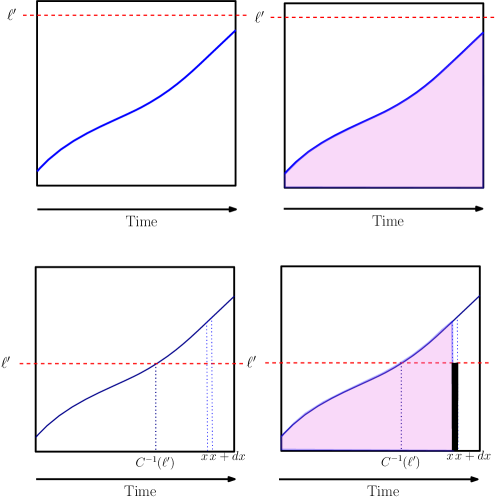
Figure 2: The two cases of Lemma 4. The blue curve is the $C$ curve.

Lemma 4.

The competitive ratio $c$ of the algorithm that follows curve $C:[0,1]\to\mathbb{R}_{\geq 0}$ satisfies

$$c\geq\min\left({1-e^{-\int_{0}^{1}C(x)dx},\min_{0<\ell^{\prime}\leq C(1)}\left({\frac{1-e^{-\int_{0}^{C^{-1}(\ell^{\prime})}C(x)dx}+\int_{C^{-1}(\ell^{\prime})}^{1}\ell^{\prime}e^{-\int_{0}^{x}C(y)dy}dx}{1-e^{-\ell^{\prime}}}}\right)}\right)$$ (1)

Proof:

Throughout the proof, see Figure 2. Recall that $C$ is an increasing curve. We abuse notation and set $C^{-1}(\ell^{\prime})=1$ for $\ell^{\prime}>C(1)$ and $C^{-1}(\ell^{\prime})=0$ for $\ell^{\prime}<C(0)$. Let ALG be the value returned by the strategy following $C$.

For $\ell\in[0,\Xi(C(1))]$, we will trivially upper bound $\mathop{\mathbb{P}}\left[{Z\geq\ell}\right]\leq 1$. Letting $U=\{(x,y)|0\leq x\leq 1,\tau_{C}(x)\leq y\leq+\infty\}$, then

$$\left|{U}\right|=\sum_{i=1}^{n}\mathop{\mathbb{P}}\left[{X_{i}\text{ arrives in }U}\right]=\sum_{i=1}^{n}\int_{0}^{1}\mathop{\mathbb{P}}\left[{X_{i}\geq\tau_{C}(x)}\right]dx=\int_{0}^{1}\sum_{i=1}^{n}\mathop{\mathbb{P}}\left[{X_{i}\geq\tau_{C}(x)}\right]dx=\int_{0}^{1}C(x)dx$$

Hence,

$$\mathop{\mathbb{P}}\left[{{\textsf{ALG}}\geq\ell}\right]=1-\mathop{\mathbb{P}}\left[{U\text{ has no arrivals}}\right]=1-e^{-\int_{0}^{1}C(x)dx}$$

For $\ell\in[\Xi(C(1)),+\infty)$, letting $U=\{(x,y)|0\leq x\leq 1,\ell\leq y<+\infty\}$, and $\ell^{\prime}=\sum_{i=1}^{n}\mathop{\mathbb{P}}\left[{X_{i}\geq\ell}\right]=\left|{U}\right|$, we have similarly that

$$\mathop{\mathbb{P}}\left[{Z\geq\ell}\right]=1-\mathop{\mathbb{P}}\left[{U\text{ has no arrivals}}\right]=1-e^{-\ell^{\prime}}$$

On the other hand, we have

$$\mathop{\mathbb{P}}\left[{{\textsf{ALG}}\geq\ell}\right]=1-e^{-\int_{0}^{C^{-1}(\ell^{\prime})}C(x)dx}+\int_{C^{-1}(\ell^{\prime})}^{1}\ell^{\prime}e^{-\int_{0}^{x}C(y)dy}dx$$

The above equality requires unpacking, see the second row of Figure 2. First, if the region $A=\{(x,y)|0\leq x\leq\tau_{C}^{-1}(\ell),\tau_{C}(x)\leq y<+\infty\}$ is non-empty (i.e. contains a realization), then the algorithm returns a value at least $\ell$. We have that

$$\left|{A}\right| =\sum_{i=1}^{n}\mathop{\mathbb{P}}\left[{X_{i}\text{ falls in }A}\right]=\sum_{i=1}^{n}\int_{0}^{\tau_{C}^{-1}(\ell)}\mathop{\mathbb{P}}\left[{X_{i}\geq\tau_{C}(x)}\right]dx$$

$$=\int_{0}^{C^{-1}(\sum_{i=1}^{n}\mathop{\mathbb{P}}\left[{X_{i}\geq\ell}\right])}\sum_{i=1}^{n}\mathop{\mathbb{P}}\left[{X_{i}\geq\tau_{C}(x)}\right]dx=\int_{0}^{C^{-1}(\ell^{\prime})}C(x)dx$$

Otherwise, for time $x\in[C^{-1}(\ell^{\prime}),1]$, if the area from time $0$ to time $x$ under curve $C$ is empty, the area from $x$ to $x+dx$ has a realization above $\ell$, then the Algorithm returns a value above $\ell$. This happens with probability $\int_{C^{-1}(\ell^{\prime})}^{1}\ell^{\prime}e^{-\int_{0}^{x}C(y)dy}dx$.

Hence, by the majorization technique discussed earlier, the competitive ratio can be lower bounded by

$$c\geq\min\left({\frac{1-e^{-\int_{0}^{1}C(x)dx}}{1},\min_{0<\ell^{\prime}\leq C(1)}\left({\frac{1-e^{-\int_{0}^{C^{-1}(\ell^{\prime})}C(x)dx}+\int_{C^{-1}(\ell^{\prime})}^{1}\ell^{\prime}e^{-\int_{0}^{x}C(y)dy}dx}{1-e^{-\ell^{\prime}}}}\right)}\right)$$

 

Simple curves evaluate well for Eq. (1). Recall, the optimal $n$ threshold algorithm for the IID case attains a competitive ratio $\approx 0.745$.

By considering simple step function curves (i.e from time $0$ to $1/m$, we use $\Xi(c_{1})$ for some constant $c_{1}$. From time $1/m$ to $2/m$, we use $\Xi(c_{2})$ for some constant $c_{2}$, and so on), evaluating the expression becomes a simple summation, since the integrals are now summations, and we can get $\approx 0.7406$ competitive ratio with $m=10$, almost matching the $\approx 0.745$ IID ratio. See Appendix B for the code and exact values of $c_{1},...,c_{m}$ we use. However, we can show that there is a function $C^{\ast}$ that attains exactly $\approx 0.745$-competitive ratio.

Lemma 5.

There exists a threshold function $C(x)$ that gives a competitive ratio of $\approx 0.745$ for the IID prophet inequality.

Proof:

We will relax the optimization from Eq. (1). Let $\tau=C^{-1}(\ell^{\prime})$, and define

$$\phi(\tau,\ell^{\prime})=1-e^{-\int_{0}^{\tau}C(x)dx}+\int_{\tau}^{1}\ell^{\prime}e^{-\int_{0}^{x}C(y)dy}dx-c(1-e^{-\ell^{\prime}})$$

We relax the optimization to requiring $\min_{0\leq\tau\leq 1,0<\ell^{\prime}}\phi(\tau,\ell^{\prime})\geq 0$ for some competitive ratio $c$. We first optimize for $\ell$’. Define $g(z)=\frac{1}{c}\int_{z}^{1}e^{-\int_{0}^{x}C(y)dy}dx$. Then $g^{\prime}(z)=-\frac{1}{c}e^{-\int_{0}^{z}C(y)dy}$. Then we have

$$\frac{\partial\phi}{\partial\ell^{\prime}}=\int_{\tau}^{1}e^{-\int_{0}^{x}C(y)dy}dx-ce^{-\ell^{\prime}}=cg(\tau)-ce^{-\ell^{\prime}}$$

Setting this to $0$, and substituting into $\phi$, we get

$$\Phi(\tau)=1+cg^{\prime}(\tau)-c\log(g(\tau))g(\tau)-c+cg(\tau)$$

The remainder of the proof follows [Sin18] in showing that the differential equation $\Phi(\tau)=0$ is satisfied for $c\approx 0.745$ (the IID constant) for some $g^{\ast}(.)$. Finally, we have

$$C(z)=-\frac{\partial^{2}g^{\ast}/\partial z^{2}}{\partial g^{\ast}/\partial z}.$$

The function $C^{\ast}(x)$ for $c=0.74544$ is shown in Figure 3.  

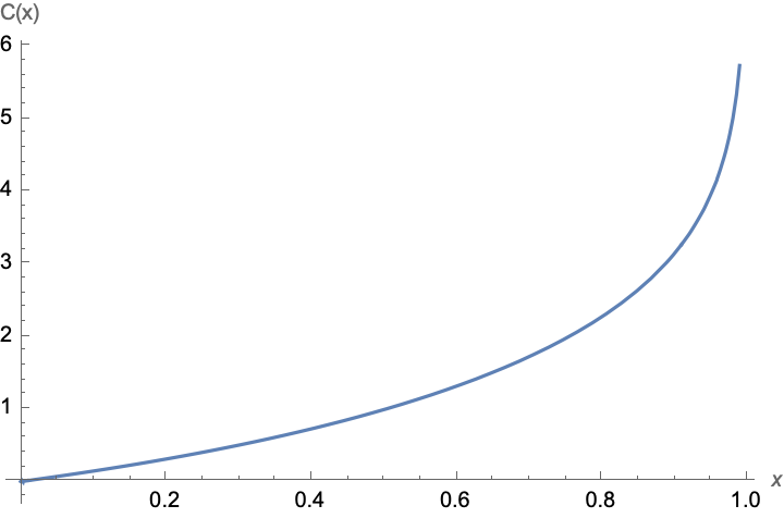
Figure 3: The function $C^{\ast}(x)$ for $c=0.745$ solved using numerical methods. The plot is truncated at $x=0.99$.

Independence of $n$

This above section shows that algorithms that are based on thresholds of the form $\sum_{i}\mathop{\mathbb{P}}\left[{X_{i}\geq\tau}\right]=q_{i}$ are comparable to algorithm that choose their thresholds based on the maximum distribution (i.e. quantiles of $Z$), at least for the iid case. One interesting fact about the result above is that the curve is independent of $n$. This is because we are approximating a continuous curve, that is independent of $n$. In particular, the $m=10$ thresholds holds for all sufficiently large $n$.

5 Prophet Secretary Non-IID Case

We now go back to the non iid case. In [CSZ20], Correa, Saona, and Ziliotto used Schur-convexity to study a class of algorithms known as blind algorithms. In particular, they consider discrete blind algorithms. The algorithm is characterized by a decreasing threshold function $\alpha:[0,1]\to[0,1]$. Letting $\mathsf{q}_{Z}\left({q}\right)$ denote the $q$-th quantile of the maximum distribution (i.e. $\mathop{\mathbb{P}}\left[{Z\leq\mathsf{q}_{Z}\left({q}\right)}\right]=q$), the algorithm accepts realization $x_{i}$ if $x_{i}\geq\mathsf{q}_{Z}\left({\alpha(i/n)}\right)$ (i.e. if it is in the top $\alpha(i/n)$ quantile of $Z$). They characterized the competitive ratio $c$ of an algorithm that follows threshold function $\alpha$ (as $n\to\infty$) as

$$c\geq\min\left({1-\int_{0}^{1}\alpha(x)dx,\min_{x\in[0,1]}\left({\int_{0}^{x}\frac{1-\alpha(y)}{1-\alpha(x)}dy+\int_{x}^{1}e^{\int_{0}^{y}\log\alpha(w)dw}dy}\right)}\right)$$ (2)

Looking at Eq. (2), the reader might already see many parallels with Eq. (1), even though one is based on quantiles of the maximum, and the other is based on summation thresholds. Correa et al. resorted to numerically solving a stiff, nontrivial optimal integro-differential equation. They find an $\alpha$ function such that $c\geq 0.665$ (and then resorted to other similar techniques to show the main $0.669$ result). They also showed than no blind algorithm can achieve a competitve ratio above $0.675$.

Ideally, one would like to have algorithms that depend on summation thresholds like we did for the iid case. If each $\mathop{\mathbb{P}}\left[{X_{i}\geq\tau_{k}}\right]$ is small, as is the case for the iid case, then we can use Poissonization. Unfortunately, we can have “superstars” in the non-iid case with “large” $\mathop{\mathbb{P}}\left[{X_{i}\geq\tau_{k}}\right]$ that mess up the error term in the coupling argument: indeed, it is no longer sufficient to use a Poisson distribution to count the number of arrivals in a region because of the non-iid nature of the random variables. What can we do then?

The main idea is to think about “breaking” each random variable $X_{i}$ with CDF $F_{i}$ into $K$ shards. More formally, we consider the iid random variables $Y_{i,1},...,Y_{i,K}$ with CDF $F_{i}^{1/K}$. This is an idea that was implicitly used in [EHLM19]. Each shard chooses a random time of arrival uniformly from $0$ to $1$ independently. One can easily see that the distribution of $\max(Y_{i,1},\ldots,Y_{i,K})$ is the same as $X_{i}$, and so the event of sampling from $X_{i}$ and choosing a random time of arrival is the same as sampling from the shards, and taking the shard with the maximum value (and its time of arrival) as the value and time of arrival for $X_{i}$.

One important subtlety about shards is that the maximum value shard in any shards realization always corresponds to an actual realization of $X_{i}$. This is because it is not dominated by any other shard (and so $X_{i}$ would take its value and time of arrival as its value).

Shards have a small probability of being above a threshold as $K\to\infty$ because $1-F^{1/K}(\tau)$ goes to $0$, and hence the coupling argument for the iid case also works. Indeed, the reader can repeat the argument from Lemma 3 and get a similar bound on the variational distance that is $0$ as $K\to+\infty$ (without any assumptions on $n$). However, the relationship between summation based thresholds on the shards $\{Y_{i,j}\}$ and maximum-based thresholds for the actual realizations $\{X_{i}\}$ is not clear. The connection is made in the following lemma.

Lemma 6.

Consider a summation based threshold on the shards that chooses threshold $\tau$ such that $\sum_{i=1}^{n}\sum_{j=1}^{K}\mathop{\mathbb{P}}\left[{Y_{i,j}\geq\tau}\right]=q$. Then as $K\to+\infty$, we have $\mathop{\mathbb{P}}\left[{Z\leq\tau}\right]=e^{-q}$.

Proof:

Because $Y_{i,j}$ are iid for fixed $i$, then we have $\sum_{i=1}^{n}K\mathop{\mathbb{P}}\left[{Y_{i,1}\geq\tau}\right]=q$. However, recall that $\mathop{\mathbb{P}}\left[{Y_{i,1}\geq\tau}\right]=1-\mathop{\mathbb{P}}\left[{X_{i}\leq\tau}\right]^{1/K}$. Hence, we are choosing a threshold such that

$$\sum_{i=1}^{n}K(1-\mathop{\mathbb{P}}\left[{X_{i}\leq\tau}\right]^{1/K})=q$$

What happens when we take $K\to\infty$? The limit of $K(1-x^{1/K})$ as $K\to\infty$ is $-\log x$. And so we have that for $K\to\infty$, $\sum_{i=1}^{n}-\log\mathop{\mathbb{P}}\left[{X_{i}\leq\tau}\right]=q$. This implies $-\log\mathop{\mathbb{P}}\left[{Z\leq\tau}\right]=q$. In other words, we chose a threshold such that $\mathop{\mathbb{P}}\left[{Z\leq\tau}\right]=e^{-q}$.  

Hence, we retrieve maximum based thresholds, but with a twist: we now have an alternative view in terms of shards. Specifically, if we choose a thresholds $\tau_{j}$ such that $\mathop{\mathbb{P}}\left[{Z\leq\tau_{j}}\right]=\alpha_{j}$, then the number of shards above $\tau_{j}$ follows a Poisson distribution with rate $\log\frac{1}{\alpha_{j}}$. This is only possible because the probability of each shard being above $\tau_{j}$ is small (i.e $\to 0$ as $K\to\infty$).

To signify the importance of this view and to warmup, we reprove several known results in the literature with this new point of view. None of these results are needed for our new results, however, they provide a much needed warmup for the sharding machinery.

5.1 Short proof of the $1-1/e$ competitive single threshold.

Lemma 7.

For the prophet secretary problem, consider the single threshold algorithm that chooses $\tau$ such that $\mathop{\mathbb{P}}\left[{Z\leq\tau}\right]=1/e$ and accepts the first value (if any) above $\tau$. Then the algorithm has a $1-1/e$ competitive ratio.

Proof:

Let us shard the $n$ random variables. Using Lemma 6, we have that $\sum_{i=1}^{n}\sum_{j=1}^{K}\mathop{\mathbb{P}}\left[{Y_{ij}\geq\tau}\right]=q=\log(e)=1$.

For $\ell\in[0,\tau]$, we have that the algorithm accepts a value $\geq\ell$ if and only if there is at least one shard above $\tau$. Hence,

$$\frac{\mathop{\mathbb{P}}\left[{{\textsf{ALG}}\geq\ell}\right]}{\mathop{\mathbb{P}}\left[{Z\geq\ell}\right]}\geq\mathop{\mathbb{P}}\left[{{\textsf{ALG}}\geq\ell}\right]=1-e^{-q}=1-\frac{1}{e}.$$

Similarly, for $\ell\in[\tau,+\infty)$, suppose the region $[0,1]\times[\tau,\ell]$ has $\beta$ shards, and the region $[0,1]\times[\ell,+\infty)$ is non empty (has some shards). Then if the maximum value shard in $[0,1]\times[\ell,+\infty)$ arrives before all $\beta$ shards, then the algorithm would accept a value above $\ell$. Letting $\ell^{\prime}=\sum_{i=1}^{n}\sum_{j=1}^{K}\mathop{\mathbb{P}}\left[{Y_{ij}\geq\ell}\right]$, we get

$$\frac{\mathop{\mathbb{P}}\left[{{\textsf{ALG}}\geq\ell}\right]}{\mathop{\mathbb{P}}\left[{Z\geq\ell}\right]}=\frac{\mathop{\mathbb{P}}\left[{{\textsf{ALG}}\geq\ell}\right]}{1-e^{-\ell^{\prime}}}\geq\frac{\sum_{\beta=0}^{\infty}(1-e^{-\ell^{\prime}})e^{-(q-\ell^{\prime})}\frac{(q-\ell^{\prime})^{\beta}}{\beta!}\frac{1}{\beta+1}}{1-e^{-\ell^{\prime}}}=\frac{e-e^{\ell^{\prime}}}{e-e\ell^{\prime}}$$

This is increasing, and is minimized in $(0,1]$ for $\ell^{\prime}\to 0$, with value $1-1/e$.

Combining both results with stochastic dominance yields the result.  

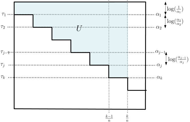
(a) Proof of Lemma 8. The region $U$ is the light
blue region.

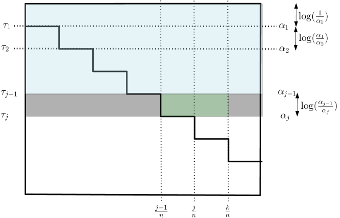
(b) The light blue region is $A_{j}$, the gray (and green) region is $B_{j}$, and the green region is where $v$ arrives.

Figure 4:

5.2 Simpler proof of key inequalities from discrete blind strategies

Next, we re-prove the following results that were proven in [CSZ20] via a nontrivial argument that applies a Schur-convexity inequality an infinite number of times. The short proof below establishes the same results via the new shards point of view.

Lemma 8.

[CSZ20] Let $T\in[n]$ be a random variable for the time that the algorithm following thresholds $\tau_{1}\geq\ldots\geq\tau_{n}$ selects a value (if any) with $\mathop{\mathbb{P}}\left[{Z\leq\tau_{j}}\right]=\alpha_{j}$. Then for any $k\in[n]$

$$\mathop{\mathbb{P}}\left[{T>k}\right]\geq\left({\prod_{j=1}^{k}\alpha_{j}}\right)^{1/n}$$

Proof:

See Figure 4(a) throughout this proof. Note that $T>k$ if and only if there are no realizations (in terms of $X_{i}$) above $\tau_{1},...,\tau_{k}$. Consider the event $\xi$ of there being no shards above $\tau_{1},...,\tau_{k}$. Then this implies that there are no realizations (in terms of $X_{i}$s) above $\tau_{1},\ldots,\tau_{k}$ and hence $\mathop{\mathbb{P}}\left[{T>k}\right]\geq\mathop{\mathbb{P}}\left[{\xi}\right]$. Now consider the area $U$ above $\tau_{1},\ldots,\tau_{k}$ between time $0$ and $\frac{k}{n}$. Letting $\alpha_{0}=1$, the measure for the region is a telescoping sum:

$$\left|{U}\right|=\sum_{i=1}^{k}\frac{k-i+1}{n}\left({\log(\frac{1}{\alpha_{i}})-\log(\frac{1}{\alpha_{i-1}})}\right)=\sum_{i=1}^{k}\frac{1}{n}\log(\frac{1}{\alpha_{j}})=\frac{1}{n}\log\left({\frac{1}{\prod_{i=1}^{k}\alpha_{i}}}\right)$$

So

$$\mathop{\mathbb{P}}\left[{\xi}\right]=e^{-\left|{U}\right|}=\left({\prod_{i=1}^{k}\alpha_{i}}\right)^{1/n}$$

 

[CSZ20] also prove the following inequality. We can also prove the same inequality via an event on the shards that implies $T\leq k$ and whose probability is the RHS.

Lemma 9.

Let $T\in[n]$ be a random variable for the time that the algorithm following thresholds $\tau_{1}\geq\ldots\geq\tau_{n}$ selects a value (if any) with $\mathop{\mathbb{P}}\left[{Z\leq\tau_{j}}\right]=\alpha_{j}$. Then for any $k\in[n]$

$$\mathop{\mathbb{P}}\left[{T\leq k}\right]\geq\frac{1}{n}\sum_{j=1}^{k}\left({1-\alpha_{j}}\right)$$

Proof:

Formally, consider the event $\xi$ where for some $1\leq j\leq k$, the region $A_{j}=\{(x,y)|0\leq x\leq 1,\tau_{j-1}\leq y<\infty\}$ is empty, and the region $B_{j}=\{(x,y)|0\leq x\leq 1,\tau_{j}\leq y\leq\tau_{j-1}\}$ is non-empty, and the maximum value shard in $B_{j}$ arrives from $t=(j-1)/n$ to $t=k/n$. See Figure 4(b).

Informally, this is the event where the region from $[\tau_{1},+\infty)$ has a shard (i.e is non empty), and the maximum shard amongst them lies from time $t=0$ to $t=k/n$, or the the region $[\tau_{1},+\infty)$ is empty, the region $[\tau_{2},\tau_{1}]$ has shards, and the maximum shard in the region lies from time $t=1/n$ to $t=k/n$, or the region $[\tau_{2},+\infty)$ is empty, the region from $[\tau_{3},\tau_{2}]$ has shards, and the maximum shard in that region arrives from time $t=2/n$ to $t=k/n$, and so on. This event implies $T\leq k$ since at least one realization would exists above $\tau_{1},...,\tau_{k}$. The probability of this event is

$$\mathop{\mathbb{P}}\left[{\xi}\right] =\sum_{i=0}^{k-1}e^{-s_{i}}(1-e^{-r_{i}})\frac{k-i}{n}$$ (3)

$$r_{i} =\log(\frac{1}{\alpha_{i+1}})-\log(\frac{1}{\alpha_{i}})$$ (4)

$$s_{i} =\sum_{j=0}^{i-1}r_{j}$$ (5)

Here, $r_{i}$ denotes the shards Poisson rate between $\tau_{i}$ and $\tau_{i+1}$, and $s_{i}$ represents the area (measure) from $\tau_{i+1}$ to $\tau_{0}=+\infty$. Simplifying via telescoping sums, we have $s_{i}=\log\frac{1}{\alpha_{i}}$, and hence we have

$$\mathop{\mathbb{P}}\left[{\xi}\right]=\sum_{i=0}^{k-1}\alpha_{i}(1-\frac{\alpha_{i+1}}{\alpha_{i}})\frac{k-i}{n}=\sum_{i=0}^{k-1}(\alpha_{i}-\alpha_{i+1})\frac{k-i}{n}=\frac{1}{m}\sum_{i=0}^{k-1}1-\alpha_{i+1}=\frac{1}{n}\sum_{i=1}^{k}1-\alpha_{i}$$

 

5.3 New analysis for the Non-IID Case

Algorithm

With the shards machinery we have built so far and the warmup above, we can now present the new analysis. Our algorithm will be a simple $m=16$ threshold algorithm following a threshold function $\tau:[0,1]\to\mathbb{R}_{\geq 0}$. From time $\frac{i-1}{m}$ to time $\frac{i}{m}$ for $1\leq i\leq m$, $\tau$ is defined to be equal to $\tau_{i}$ with $\tau_{1}>\ldots>\tau_{m}$ (i.e $\tau$ is a step function). We accept the first realization $(t_{i},x_{i})$ with $x_{i}\geq\tau(t_{i})$.

Lemma 10.

The competitive ratio $c$ satisfies

$$c\geq\min_{1\leq j\leq m+1}\min_{\alpha_{j}\leq\alpha_{t}\leq\alpha_{j-1}}\frac{f_{j}({\boldsymbol{\alpha}},\alpha_{t})}{1-\alpha_{t}}$$ (6)

Where

$$f_{j}({\boldsymbol{\alpha}},\alpha_{t}) =\frac{1}{m}\sum_{k=1}^{j-1}\left({1-\alpha_{k}}\right)+\sum_{k=j}^{m}\left({\prod_{\nu=1}^{k-1}\alpha_{\nu}}\right)^{\frac{1}{m}}w_{k}q_{t,k}$$ (7)

$$w_{k} =\sum_{\nu=0}^{j-1}e^{-s_{\nu}}(1-e^{-r_{\nu}})\frac{1}{m-(k-1)+\nu}$$ (8)

$$r_{\nu} =\frac{m-(k-1)+\nu}{m}\log\frac{\hat{\alpha}_{\nu}}{\hat{\alpha}_{\nu+1}}$$ (9)

$$\hat{\alpha_{\nu}} =\alpha_{\nu}\text{ if }\nu\leq j-1\text{ and }\alpha_{t}\text{ if }\nu=j$$ (10)

$$s_{\nu} =\sum_{\beta=0}^{\nu-1}r_{\beta}$$ (11)

$$q_{t,k} =\sum_{\beta=0}^{+\infty}e^{-\frac{1}{m}\log\frac{\alpha_{t}}{\alpha_{k}}}\left({\frac{1}{m}\log\frac{\alpha_{t}}{\alpha_{k}}}\right)^{\beta}\frac{1}{\beta!}\frac{1}{\beta+1}=\frac{1-\left({\frac{\alpha_{k}}{\alpha_{t}}}\right)^{1/m}}{\frac{1}{m}\log\left({\frac{\alpha_{t}}{\alpha_{k}}}\right)}$$ (12)

Proof:

We would like to compare $\mathop{\mathbb{P}}\left[{Z\geq\ell}\right]$ vs $\mathop{\mathbb{P}}\left[{{\textsf{ALG}}\geq\ell}\right]$ as before. For this, we again break the analysis on where $\ell$ lies.

For $\ell\in[0,\tau_{m})$

See Figure 5. We use the trivial upper bound $\mathop{\mathbb{P}}\left[{Z\geq\ell}\right]\leq 1$. On the other hand, consider when ${\textsf{ALG}}\geq\ell$. Using Lemma 9, we have $\mathop{\mathbb{P}}\left[{{\textsf{ALG}}\geq\ell}\right]\geq\frac{1}{m}\sum_{i=1}^{m}\left(1-\alpha_{i}\right)$. Hence

$$\frac{\mathop{\mathbb{P}}\left[{{\textsf{ALG}}\geq\ell}\right]}{\mathop{\mathbb{P}}\left[{Z\geq\ell}\right]}\geq\frac{1}{m}\sum_{i=1}^{m}\left(1-\alpha_{i}\right)$$

This case is handled by $f_{m+1}({\bf\alpha},\alpha_{t})$.

The case of $\ell\in[\tau_{j},\tau_{j-1}]$

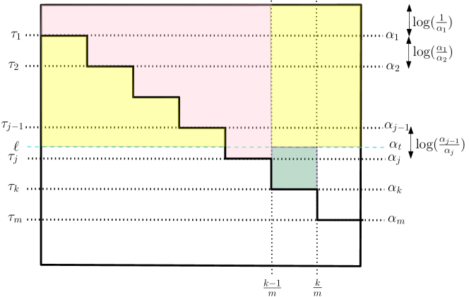
Figure 5: Analysis visualization of Section 5.3

Again, see Figure 5. Let $\alpha_{t}=\mathop{\mathbb{P}}\left[{Z\leq\ell}\right]$. We know $\alpha_{j}\leq\alpha_{t}\leq\alpha_{j-1}$. We also know $\mathop{\mathbb{P}}\left[{Z>\ell}\right]=1-\alpha_{t}$. Now, we want to compute the probability that ${\textsf{ALG}}\geq\ell$. We again give an event $\xi$ on the shards that implies ${\textsf{ALG}}\geq\ell$ and with $\mathop{\mathbb{P}}\left[{\xi}\right]=f_{j}({\bf\alpha},\alpha_{t})$. We recommend looking at Figure 5 throughout the explanation.

Formally, $\xi$ consists of a disjoint union of $m-j+2$ events. The first event $\chi$ is the event that $T\leq j-1$. The next $m-j+1$ events $\eta_{k},j\leq k\leq m$ is such that event $\eta_{k}$ is that there are no shards above $\tau_{1},...,\tau_{k-1}$ (the pink region in Figure 5), that there are shards above $\ell$ (the yellow region in Figure 5), and that the maximum value shard $v$ from the yellow shards arrives between time $t=(k-1)/m$ to $t=k/m$, and that $v$’s time of arrival is before all the shards that appear from $t=(k-1)/m$ to $t=k/m$ between $\tau_{k}$ and $\ell$ (the green region in Figure 5).

From Lemma 9, the probability of $\chi$ happening is at least $\frac{1}{m}\sum_{k=1}^{j-1}1-\alpha_{k}$. This would also correctly imply ${\textsf{ALG}}\geq\ell$.

First, on why $\{\eta_{k}\}$ events imply ${\textsf{ALG}}\geq\ell$. If there are no shards above $\tau_{1},...,\tau_{k-1}$ (pink region) then this implies $T\geq k$. If there are shards above $\ell$ (in the yellow region) and the maximum shard falls from $t=(k-1)/m$ to $t=k/m$ then there is at least one realization $v$ (from $X_{i}$s) that is between $t=(k-1)/m$ to $t=k/m$. If $v$ arrives before all shards between $\tau_{k}$ and $\ell$ between time $(k-1)/m$ and $k/m$ (i.e green region), then the realization corresponding to $v$ would be chosen by the Algorithm before any potential realization corresponding to the shards between $\tau_{k}$ and $\ell$. Hence, ${\textsf{ALG}}\geq\ell$.

Breaking the RHS further, for fixed $k$, the first term $\left({\prod_{\ell=1}^{k-1}\alpha_{\ell}}\right)^{\frac{1}{m}}$ term computes the probability that there are no shards in the first $k-1$ thresholds as seen in Lemma 8. The second term $w_{k}$ computes the probability that the shard with maximum value (in the yellow region) falls between $t=(k-1)/m$ to $t=k/m$, and multiplies that by $q_{t,k}$ which is the probability that this maximum shard appears before any shards between $t=(k-1)/m$ and $t=k/m$ and with value between $\tau_{k}$ and $\ell$ (the green region).

One last remark is on using $\hat{\alpha_{i}}$ vs $\alpha_{i}$. There is a corner case in the summations where we should use $\alpha_{t}$ instead of $\alpha_{j}$, and so represent this conditional usage using $\hat{\alpha_{i}}$.  

Optimization

The right hand side of Eq. (6) can be maximized for $\boldsymbol{\alpha}$ satisfying $\alpha_{0}=1>\alpha_{1}>\ldots>\alpha_{m}>\alpha_{m+1}=0$. We used Python to optimize the expression and report $m=16$ alpha values in Appendix C with $c\geq 0.6724$. We also provide our Python code in the appendix as a tool to help the reader verify our claims. A lot of effort was spent to make sure the naming and indexing used in the paper match the code identically to help a skeptic reader verify the claim. All computations were done with doubles using a precision of 500 bits (instead of the default 64).

Remark 5.1.

The function $\frac{1-\left({\frac{\alpha_{k}}{\alpha_{t}}}\right)^{1/m}}{\frac{1}{m}\log\left({\frac{\alpha_{t}}{\alpha_{k}}}\right)}$ in Eq. (12) is numerically unstable for close values of $\alpha_{k},\alpha_{t}$. To resolve this, we lower bound it by truncating the summation on the LHS to $30$ terms (instead of $\infty$) and use that as a lower bound on $q_{t,k}$. This is refered to as “stable_qtk” in the code.

We finally get the main result.

Theorem 5.2.

There exists an $m=16$ threshold blind strategy for the prophet secretary problem that achieves a competitive ratio of at least $0.6724$.

Parameter optimization is not sufficient

Why does the above analysis yield a better competitive ratio for continious blind strategies? It is important to stress that the set of $m=16$ parameters we derive would not improve the analysis from [CSZ20] from $0.669$ to $0.6724$; in fact, they give a worse bound of $0.6675$! In particular, the constants $f_{j}({\bf\alpha},\alpha_{t})$ we derive are significantly tighter than the $f_{j}(\alpha_{1},...,\alpha_{m})$ that Correa et al. derive. This is because the new bounds utilize all aspects of the geometry involved. In contrast, the work in [CSZ20] attempted to do this separately using algebraic tools, but were unable to derive customized upper bounds for every single $f_{j}(\alpha_{1},...,\alpha_{m})$. Hence we are optimizing for different objectives.

6 IID Semi-Online

In this section, we improve the $\approx 0.869$ competitive ratio result from [HS23] and give a $\approx 0.89$ competitive ratio algorithm for the IID Semi-Online problem.

It is worth taking a moment to recap the algorithm from [HS23]. As a reminder, the algorithm would use thresholds $\{t_{i}\}$ to ask $X_{1},...,X_{n}$ if $X_{i}\geq t_{i}$, and update the thresholds adaptively based on the response. Their algorithm defines thresholds $\tau_{1}<\tau_{2}<\tau_{3}<\tau_{4}=+\infty$. It then runs the following algorithm:

1. Set $r\leftarrow 1$ and $i^{\ast}\leftarrow 1$

2. For $i=1,...,n$:

3. If $X_{i}\geq\tau_{r}$:

4. $r\leftarrow r+1$ and $i^{\ast}\leftarrow i$

5. Return $X_{i}^{\ast}$

Intuitively, the algorithm “raises” the threshold it uses every time it gets a positive response for a query, aiming for a higher conditional expectation. [HS23] optimize the parameters as quantiles of the maximum and choose $\tau_{1}=\Xi(2.035135),\tau_{2}=\Xi(0.5063),\tau_{3}=\Xi(0.05701)$ which yields a $\approx 0.869$ competitive algorithm using stochastic dominance/majorization. Note that the analysis for $\mathop{\mathbb{P}}\left[{{\textsf{ALG}}\geq\ell}\right]$ is quite subtle, because even if we see a realization with a value above $\ell$, there might be a subsequent realization above a later threshold but below $\ell$, at which case the last successful realization is below $\ell$. In other words, we must insure that the last realization that succeeds (i.e gets a “yes” response) is above $\ell$.

The problem with the existing algorithm is that if (say) the first $n/2$ tests are below $\tau_{1}$, it is unlikely that the later realizations will show up above $\tau_{1}$. Hence, it is unlikely to get even a single success later on in the algorithm and we end up not using $\tau_{2},\tau_{3}$.

To combat this, we adopt the same strategy, but (perhaps counter-intuitively) with non-increasing functions instead. In particular, we define $k$ non-increasing functions $\tau_{1},\tau_{2},...,\tau_{k}:[0,1]\to\mathbb{R}_{\geq 0}$, and with $\tau_{k+1}=+\infty$. We then run the above algorithm, but replacing line 3 with “If $X_{i}\geq\tau_{r}(t_{i})$” where $t_{i}$ is the time of arrival of $X_{i}$.

To start off, analyzing this algorithm in a standard way would be quite challenging, and full of case by case analysis. This is because there is dependence once you condition that there is $t$ points in some quantile range of the distribution, and multiple nested summations quickly arise. Indeed, even using constant functions (the result from [HS23]) is quite technical even for two thresholds.

In this section, we show how using Poissonization and dynamic programming, we are able to lower bound the competitive ratio. Note that the result in [HS23] assumes $n\to+\infty$, which we also assume here.

6.1 Dynamic programming to compute the competitive ratio

The algorithm

To simplify the exposition, we will have $k$ threshold functions $\tau_{1},...,\tau_{k}$ which are all decreasing step functions. In particular, for some $p\in\mathbb{N}_{\geq 1}$, from time $(i-1)/p$ to time $i/p$ for $1\leq i\leq p$, the threshold for $\tau_{j}(x)$ will be $\Xi(c_{ij})$. Hence, we are optimizing for $kp$ parameters $\{c_{i,j}\}$.

Finely Discretizing time

Even with Poissonization, the exact analysis of such strategy would still be painful and involve several nested summations. To counter this, we break time into discretized chunks of $1/m$ using a clock (with $m\in\mathbb{N}_{\geq 1}$). In particular, we use the following modified algorithm.

1. Set $r\leftarrow 1$ and $i^{\ast}\leftarrow 1$

2. clock$\leftarrow 0$

3. For $i=1,...,n$:

4. If $X_{i}\geq\tau_{r}(t_{i})$ and $t_{i}\geq\textsc{clock}$:

5. $r\leftarrow r+1$

6. $i^{\ast}\leftarrow i$

7. clock $\leftarrow\lceil mt_{i}\rceil/m$

8. Return $X_{i}^{\ast}$

In particular, once we see a value above $\tau_{r}(t_{i})$, we “skip” the time to the next multiple of $1/m$. As $m$ increases, the performance of the algorithm should mimic the continuous counterpart. We will also insure that $p|m$ so that the discretized times are aligned with the $p$ phases of any of the functions $\tau_{j}$.

Dynamic Program

Fix $\ell$, and suppose we want to compute $\mathop{\mathbb{P}}\left[{{\textsf{ALG}}\geq\ell}\right]$ to use stochastic dominance. Let $\textsc{Prob}[b,j,i]$ with $b\in\{\textsc{T},\textsc{F}\},0\leq i<m,1\leq j\leq k+1$ denote the probability that the last successful test on variables that arrive from time $t=i/m$ to $t=1$ is above $\ell$, if we are currently using threshold function $\tau_{j}$, and given that last successful query we have seen (if any) is (or is not) above $\ell$ (depending on $b=\textsc{T}$ or $b=\textsc{F}$).

For example, $\textsc{Prob}[\textsc{T},2,120]$ denotes the probability that the last successful test on variables that arrive from time $t=120/m$ to $t=1$ are above $\ell$ if we are currently using threshold function $\tau_{2}$, and given that the last successful query was above $\ell$. Clearly, $\textsc{Prob}[\textsc{F},1,0]=\mathop{\mathbb{P}}\left[{{\textsf{ALG}}\geq\ell}\right]$.

Recurrence

Lemma 11.

Let $C[j,i]=\sum_{\beta=1}^{n}\mathop{\mathbb{P}}\left[{X_{\beta}\geq\tau_{j}(i/m)}\right]$ and $\ell^{\prime}=\sum_{\beta=1}^{n}\mathop{\mathbb{P}}\left[{X_{i}\geq\ell}\right]$. To compute $\textsc{Prob}[b,i,j]$, if $i\geq m$ or $j=k+1$, then $\textsc{Prob}[\textsc{True},i,j]=1$ and $\textsc{Prob}[\textsc{False},i,j]=0$. Otherwise, we have the recurrence

$$\textsc{Prob}[b,j,i] =\begin{cases}e^{-\frac{C[j,i]}{m}}\textsc{Prob}[b,j,i+1]+(1-e^{-\frac{C[j,i]}{m}})\frac{\ell^{\prime}}{C[j,i]}\textsc{Prob}[\textsc{T},j+1,i+1]\\ &\text{ If }\ell^{\prime}\leq C[j,i]\\ ~{}~{}~{}~{}~{}~{}~{}~{}~{}~{}~{}~{}~{}~{}~{}~{}~{}~{}~{}~{}~{}~{}~{}~{}~{}~{}~{}~{}~{}~{}+(1-e^{-\frac{C[j,i]}{m}})\frac{C[j,i]-\ell^{\prime}}{C[j,i]}\textsc{Prob}[\textsc{F},j+1,i+1]\\ ~{}\\ e^{-\frac{C[j,i]}{m}}\textsc{Prob}[b,j,i+1]+(1-e^{-\frac{C[j,i]}{m}})\textsc{Prob}[\textsc{T},j+1,i+1]&\text{ If }\ell^{\prime}>C[j,i]\end{cases}$$

In particular, we can compute $\textsc{Prob}(\textsc{F},1,0)$ in $O(mk)$ time.

Before we prove Lemma 11, we need the following helper lemma.

Lemma 12.

Let $\tau_{1}=\Xi(\ell_{1})$ and $\tau_{2}=\Xi(\ell_{2})$ for $\ell_{1}<\ell_{2}$. Then

$$\mathop{\mathbb{P}}\left[{\text{The first realization above $\tau_{2}$ is also above }\tau_{1}}\middle|\;\text{There is a realization above }\tau_{2}\right]=\frac{\ell_{1}}{\ell_{2}}$$

Proof:

The conditional probability is

$$\frac{\int_{0}^{1}e^{-\ell_{2}x}\ell_{1}dx}{1-e^{-\ell_{2}}}=\frac{\ell_{1}}{\ell_{2}}$$

 

Finally, we are able to prove Lemma 11

Proof of​

Lemma 11 The base cases are clear. First, suppose $\ell^{\prime}\leq C[j,i]$. There are three cases

1. If there is no realization from $i/m$ to $(i+1)/m$ above $\tau_{j}(i/m)$ (which happens with probability $e^{-C[j,i]/m}$), then the probability is simply $\textsc{Prob}[b,j,i+1]$.

2. If there is a realization above $\tau_{j}(i/m)$ and the first realization is above $\ell$ (which happens with probability $(1-e^{-C[j,i]/m})\frac{\ell^{\prime}}{C[j,i]}$ using Lemma 12), then the last successfull test is above $\ell$, and we continue to $\tau_{j+1}$ and time $(i+1)/m$ immediately because of the clock. This corresponds to $\textsc{Prob}[\textsc{T},j+1,i+1]$.

3. If there is a realization above $\tau_{j}(i/m)$ and the first realization is below $\ell$, then the last successfull test is now below $\ell$, and we continue to $\tau_{j+1}$ from time $(i+1)/m$, which corresponds to $\textsc{Prob}[\textsc{F},j+1,i+1]$.

Finally, if $\ell^{\prime}>C[j,i]$, then if there is no realization above $\tau_{j}(i/m)$, we continue $\textsc{Prob}[b,j,i+1]$. Finally, if there is a realization, then the last realization is above $\ell$ now, and we proceed with $\textsc{Prob}[\textsc{T},j+1,i+1]$.  

Optimization

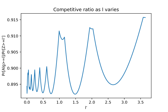
Figure 6: $\mathop{\mathbb{P}}\left[{{\textsf{ALG}}\geq\ell}\right]/\mathop{\mathbb{P}}\left[{Z\geq\ell}\right]$ for $\ell^{\prime}$ from $0$ to $\max_{i,j}(c_{i,j})$

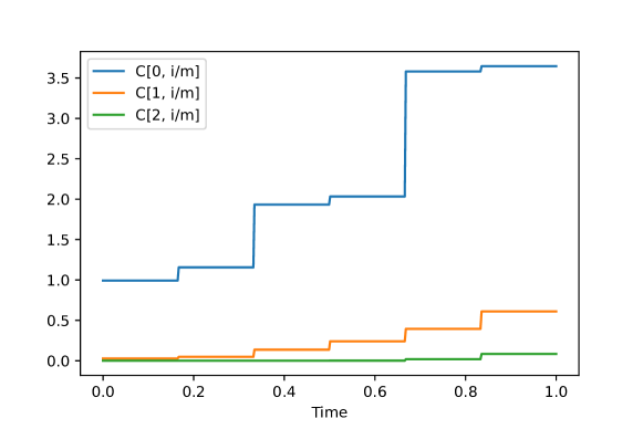
Figure 7: The threshold functions as time varries. Note that the values displayed here are the $c_{j,i}$ (i.e on expectation, this is how many points should be above the threshold function at this time). The blue, orange, and green thresholds correspond to $\tau_{1},\tau_{2},\tau_{3}$ respectively.

We set $m=420$, $p=6$, and $k=3$. Hence we are optimizing for $kp=18$ parameters. In Appendix D, we provide the set of parameters we use along with the code. For the fixed parameters, we use a global single variable optimizer (SHG optimization, or simplicial homology global optimization) to find the minima across $\ell^{\prime}\in(0,\max_{i,j}c_{i,j}]$. See Figure 6 for the plot of the competitive ratio as $\ell^{\prime}$ varries from $0$ to $\max_{i,j}(c_{i,j})$. As seen from the code and the Figure, the global optimizer correctly finds the minima at $\ell^{\prime}\approx 1.483887$.

For $\ell^{\prime}>\max_{i,j}c_{i,j}$, we upper bound $\mathop{\mathbb{P}}\left[{Z\geq\ell}\right]\leq 1$ again, and the lower bound for $\mathop{\mathbb{P}}\left[{{\textsf{ALG}}\geq\ell}\right]$ is simply at least $1-e^{-\frac{1}{m}\sum_{i=1}^{m}C[1,i]}$. Finally, we return the minimum of both values as usual. The result here is $>0.89$. See Figure 7 for the three threshold functions.

7 IID and non-IID Semi-Online-Load-Minimization

We briefly recap the problem. In this setting, we are allowed to ask $n$ queries in total, but a variable can be asked multiple queries. The maximum time any variable is asked is the load. The objective is to find a $1-o(1)$ competitive algorithm in this setting while minimizing the load. [HS23] give an algorithm with $O(\log n)$ load for IID random variables, and leave the non-IID case as a future problem.

In this section, we give a $O(\log^{\ast}n)$ load algorithm for the non-IID case, hence also improving on the IID load.

Bruteforce

If we have a small number of random variables $Y_{1},...,Y_{r}$, then we can find the maximum with $O(r)$ expected queries and $O(r)$ expected maximum load. We can find which of two random variables (say $Y_{1},Y_{2}$) are larger using $O(1)$ calls on expectation. We query with $\tau$, set to be the median of $Y_{1}$. Then with probability $1/2\mathop{\mathbb{P}}\left[{Y_{2}\geq\tau}\right]+1/2\mathop{\mathbb{P}}\left[{Y_{2}\leq\tau}\right]=1/2$, the realizations are on different sides and we are done in one iteration. However, if the query answers “yes” or “no” to both, then we update $Y_{1},Y_{2}$ to be the new conditional distributions on this information (for example, if both are “yes”, then we update the variables to be $Y_{1}|Y_{1}\geq\tau,Y_{2}|Y_{2}\geq\tau$), and repeat this process. With probability $1/2^{i}$, we are done in $i$ iterations. So after $2=O(1)$ expected calls, we know which random variable is larger. Now we apply this process iteratively to $Y_{1},...,Y_{r}$ using on expectation $O(r)$ queries and load.

Algorithm

Uniformly sample $\sigma\in\mathbb{S}_{n}$. First, we throw away $n^{\prime}=\lceil\sqrt{n}\rceil$ variables, $X_{\sigma(1)},...,X_{\sigma(n^{\prime})}$. We now have $n-n^{\prime}$ random variables $X_{\sigma(n^{\prime}+1)},...,X_{\sigma(n)}$ and an extra budget of $n^{\prime}$ queries to use for these random variables. Next, we shard the random variables $X_{\sigma(n^{\prime})},...,X_{\sigma(n)}$ into $\{Y_{\sigma(i)j}\}$. We define $\tau_{1}$ such that $\sum_{i=n^{\prime}+1}^{n}\sum_{j=1}^{K}\mathop{\mathbb{P}}\left[{Y_{\sigma(i),j}\geq\tau_{1}}\right]=c\log n$ for a sufficiently large constant $c$.

Log reduction

For $X_{\sigma(n^{\prime}+1)},...,X_{\sigma(n)}$ we first use the threshold $\tau_{1}$ described above. If at least one query answer is “yes”, then we continue to the next iteration by including only the random variables that answered yes. In iteration $t$, we use the threshold $\Xi(c\log^{(t)}n)$, the $\log$ function nested $t$ times (for example $\log^{(2)}n=\log\log n$). By sharding and Poissonization, if we are in iteration $t$, then with probability $1-e^{-c\log^{(t)}n}=1-\frac{1}{\left(\log^{(t-1)}n\right)^{c}}$, we continue to the following iteration, and with probability $\frac{1}{\left(\log^{(t-1)}n\right)^{c}}$, the answer will be “no” for all random variables being considered (since none are above the new threshold). In that case, we run the bruteforce solution using $O(\log^{(t)}n)$ queries and load on expectation. So in total, the maximum load on any random variable is on expectation

$$O(\log^{\ast}n)+\sum_{t=1}^{O(\log^{\ast}n)}\frac{O(\log^{t}n)}{O(\log^{(t-1)}n)^{c}}=O(\log^{\ast}n)$$

Clearly, the algorithm always succeeds if $X_{\sigma(n^{\prime}+1)},...,X_{\sigma(n)}$ contains the maximum realization from $X_{1},...,X_{n}$, which happens with high probability. We now make this more formal.

Lemma 13.

$$\mathop{\mathbb{E}}\!\left[{{\textsf{ALG}}}\right]\geq(1-\frac{1}{n^{O(1)}})\mathop{\mathbb{E}}\!\left[{Z}\right]$$

Where ALG is the value returned by the algorithm.

Proof:

We have that

$$\mathop{\mathbb{E}}\!\left[{{\textsf{ALG}}}\right]=\sum_{z\in[0,+\infty)}\mathbb{1}_{z\geq\tau_{1}}z\mathop{\mathbb{P}}\left[{{\textsf{ALG}}\text{ gets maximum }|Z=z}\right]$$

For $z\geq\tau_{1}$, with probability at least $\geq 1-n^{\prime}/n=1-1/n^{O(1)}$), the maximum is in $X_{\sigma(n^{\prime}+1)},...,X_{\sigma(n)}$ and the algorithm succeeds in finding it. So we have

$$\mathop{\mathbb{E}}\!\left[{{\textsf{ALG}}}\right]\geq(1-1/n^{O(1)})\sum_{z\in[0,+\infty)}\mathbb{1}_{z\geq\tau_{1}}z=(1-1/n^{O(1)})\mathop{\mathbb{P}}\left[{Z\geq\tau}\right]\mathop{\mathbb{E}}\!\left[{Z}\right]\geq(1-1/n^{O(1)})(1-1/n^{O(1)})\mathop{\mathbb{E}}\!\left[{Z}\right]$$

The result follows.  

8 Best-1-of-$k$

Improved algorithm for Best-1-of-$2$

We give an improved algorithm for the best-1-of-$2$ problem. This improves the result by Assaf and Samuel-Cahn from $\approx 0.731$ to $0.77$.

Algorithm

The algorithm is a simple two-threshold algorithm. We first shard the random variables $X_{1},...,X_{n}$ into $\{Y_{i,j}\}$. We select thresholds $\tau_{1}=\Xi(c_{1}),\tau_{2}=\Xi(c_{2})$ on the shards, for some constants $c_{1}>c_{2}$. Specifically, we choose thresholds $\tau_{1},\tau_{2}$ such that

$$\sum_{i=1}^{n}\sum_{j=1}^{K}\mathop{\mathbb{P}}\left[{Y_{i,j}\geq\tau_{i}}\right]=c_{i}$$

The algorithm accepts the first value (if any) above $\tau_{1}$, and updates the threshold to $\tau_{2}$. It finally accepts any value (if any) above $\tau_{2}$, and terminates.

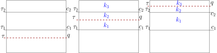
Figure 8: The 3 cases of the analysis for best-1-of-2 algorithm from left to right.

Analysis

See Figure 8 throughout the analysis. Again, we proceed by majorization. For $\tau\in[0,\tau_{1})$, we have $\mathop{\mathbb{P}}\left[{Z\geq\tau}\right]\leq 1$. Finally, if there is a shard with value above $\tau_{1}$, then the algorithm returns a value above $\tau$. So we have

$$\frac{\mathop{\mathbb{P}}\left[{{\textsf{ALG}}\geq\tau}\right]}{\mathop{\mathbb{P}}\left[{Z\geq\tau}\right]}\geq 1-e^{-c_{1}}$$

For $\tau\in[\tau_{1},\tau_{2}]$, we have that $\mathop{\mathbb{P}}\left[{Z\geq\tau}\right]=1-e^{-q}$ where $q=\sum_{i}\sum_{j}\mathop{\mathbb{P}}\left[{Y_{i,j}\geq\tau}\right]$. We have $q\in[c_{2},c_{1}]$. Finally, consider the following event on the shard that implies ${\textsf{ALG}}\geq\tau$. Let $k_{1}$ be the number of shards with values in $[\tau_{1},\tau)$, $k_{2}$ be the number of shards with values in $[\tau,\tau_{2})$, and $k_{3}$ be the number of shards with value $[\tau_{2},+\infty)$. Then if $k_{1}=0$ and $k_{2}+k_{3}\geq 1$, or $k_{1}\geq 1$ and $k_{3}\geq 1$, then ${\textsf{ALG}}\geq\tau$. For the first case, if $k_{2}+k_{3}\geq 1$, then there is at least one shard above $\tau$ corresponding to an actual realization of $\{X_{i}\}$. But since $k_{1}=0$, then this realization will be selected by the algorithm. If $k_{1}\geq 1$ and $k_{3}\geq 1$, then again, there is a shard above $\tau_{2}\geq\tau$ that corresponds to an actual realization of $\{X_{i}\}$. On a worst case, one of the $k_{1}$ shards from $[\tau_{1},\tau]$ correspond to actual realizations in $\{X_{i}\}$ and arrives first. In this case, the algorithm raises the threshold to $\tau_{2}$ (at which case, none of the other realization below $\tau$ can be selected), and the algorithm ends up selecting a value with $\geq\tau$. Hence,

$$\frac{\mathop{\mathbb{P}}\left[{{\textsf{ALG}}\geq\tau}\right]}{\mathop{\mathbb{P}}\left[{Z\geq\tau}\right]}\geq\frac{e^{-(c_{1}-q)}(1-e^{-q})+(1-e^{-(c_{1}-q)})(1-e^{-c_{2}})}{1-e^{-q}}$$

Finally, for $\tau\in[\tau_{2},+\infty)$, we have that $\mathop{\mathbb{P}}\left[{Z\geq\tau}\right]=1-e^{-q}$ where $q=\sum_{i}\sum_{j}\mathop{\mathbb{P}}\left[{Y_{i,j}\geq\tau}\right]$, with $q\in(0,c_{2}]$. Consider the following event on the shards that implies ${\textsf{ALG}}\geq\tau$. Let $k_{1}$ be the number of shards with values in $[\tau_{1},\tau_{2})$, $k_{2}$ be the number of shards with values in $[\tau_{2},\tau)$, and $k_{3}$ be the number of shards with value $[\tau,+\infty)$. If $k_{1}=0,k_{2}\in\{0,1\},k_{3}\geq 1$ or $k_{1}\geq 1,k_{2}=0,k_{3}\geq 1$, then the algorithm gets a value at least $\tau$. In the first case, there is at most one shard below $\tau$, and at least one shard above $\tau$ corresponding to a value at least $\tau$, so the algorithm selects a value above $\tau$. In the second case, if $k_{1}\geq 1,k_{2}=0$, then in a worst case, one of the $k_{1}$ values corresponds to an actual realization, at which case the algorithm raises its threshold (not accepting anything below $\tau_{2}$ anymore), and accepts the first realization above $\tau$ because $k_{3}\geq 1$. Hence,

$$\frac{\mathop{\mathbb{P}}\left[{{\textsf{ALG}}\geq\tau}\right]}{\mathop{\mathbb{P}}\left[{Z\geq\tau}\right]} \geq\frac{\left[e^{-(c_{1}-c_{2})}e^{-(c_{2}-q)}(1+c_{2}-q)+(1-e^{-(c_{1}-c_{2})})e^{-(c_{2}-q)}\right](1-e^{-q})}{1-e^{-q}}$$

$$=\left[e^{-(c_{1}-c_{2})}e^{-(c_{2}-q)}(1+c_{2}-q)+(1-e^{-(c_{1}-c_{2})})e^{-(c_{2}-q)}\right]$$

$$=e^{-c_{2}+q}+e^{-c_{1}+q}(c_{2}-q)$$

Note that $e^{-c_{2}+q}+e^{-c_{1}+q}(c_{2}-q)$ is increasing on $q\in(0,c_{2})$, because the derivative is $e^{q-c_{1}}(c_{2}-q)-e^{q-c_{1}}+e^{q-c_{2}}\geq 0$. Hence, $\min_{0<q\leq c_{2}}e^{-c_{2}+q}+e^{-c_{1}+q}(c_{2}-q)=e^{-c_{2}}+e^{-c_{1}}c_{2}$. This implies the following lemma

Lemma 14.

The competitive ratio of the best-1-of-$2$ algorithm is at least

$$\min\left(1-e^{-c_{1}},\min_{c_{2}\leq q\leq c_{1}}\left(\frac{e^{-(c_{1}-q)}(1-e^{-q})+(1-e^{-(c_{1}-q)})(1-e^{-c_{2}})}{1-e^{-q}}\right),e^{-c_{2}}+e^{-c_{1}}c_{2}\right)$$ (13)

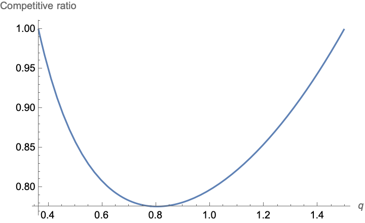
Figure 9: Value of $\left(\frac{e^{-(c_{1}-q)}(1-e^{-q})+(1-e^{-(c_{1}-q)})(1-e^{-c_{2}})}{1-e^{-q}}\right)$ as $q$ ranges from $c_{2}$ to $c_{1}$

Optimization

We select $c_{1}=1.49721,c_{2}=0.364075$ such that Eq. (13) evaluates to $0.776$. See Figure 9 for a plot of the middle term as $q$ ranges from $c_{2}$ to $c_{1}$. This implies the result

Theorem 8.1.

There is a best-1-of-$2$ algorithm that achieves a competitive ratio of at least $0.77$.

Best $1$-of-$k$

Next, we present our result for best $1$-of-$k$. We shard the variables $X_{1},...,X_{n}$ into $\{Y_{i,j}\}$. We set a single threshold $\tau_{1}$ such that

$$\sum_{i=1}^{n}\sum_{j=1}^{K}\mathop{\mathbb{P}}\left[{Y_{i,j}\geq\tau}\right]=c$$

For some constant $c$. Again, we proceed by majorization. If $\tau\in[0,\tau_{1}]$, then $\mathop{\mathbb{P}}\left[{{\textsf{ALG}}\geq\tau}\right]/\mathop{\mathbb{P}}\left[{Z\geq\tau}\right]\geq 1-e^{-c}$.

Finally, if $\tau\in[\tau_{1},+\infty)$, and $q=\sum_{i}\sum_{j}\mathop{\mathbb{P}}\left[{Y_{i,j}\geq\tau}\right]=q$ with $0<q\leq c$. Consider the number of shards with value between $\tau_{1}$ and $\tau$. If this number is at most $k-1$ and there is a shard above $\tau$, then the algorithm would successfully reach a shard above $\tau$ corresponding to an actual realization. Hence, we have

$$\frac{\mathop{\mathbb{P}}\left[{{\textsf{ALG}}\geq\tau}\right]}{\mathop{\mathbb{P}}\left[{Z\geq\tau}\right]}\geq\frac{(1-e^{-q})\sum_{i=0}^{k-1}e^{-(c-q)}\frac{(c-q)^{i}}{i!}}{1-e^{-q}}=\sum_{i=0}^{k-1}e^{-(c-q)}\frac{(c-q)^{i}}{i!}=f_{k}(c,q)$$

Note that for $q\to 0$, $f_{k}(c,q)=1-\sum_{i=k}^{\infty}e^{-c}\frac{c^{i}}{i!}$. Moreover, $\partial f_{k}(q,c)/\partial q=0$ if and only if $q=c$. When that happens, the competitive ratio is $1$. Hence $f_{k}(q,c)$ is minimized for $q\to 0$. By Taylor approximation on the function $f(x)=e^{x-c}$, we have for some $\xi\in(0,c]$

$$\sum_{i=k}^{\infty}e^{-c}\frac{c^{i}}{i!}<\frac{f^{(k)}(\xi)c^{k}}{k!}<\frac{c^{k}}{k!}$$

Finally, the competitive ratio of the algorithm is at least $\min\left(1-e^{-c},1-\frac{c^{k}}{k!}\right)$. We set $1-e^{-c}=1-\frac{c^{k}}{k!}$, which has a solution of $c=kW(\frac{\sqrt[k]{k!}}{k})$ where $W$ is the Lambert $W$ function.

Theorem 8.2.

There exists an algorithm for best-1-of-$k$ with a competitive ratio at least $1-e^{-kW(\frac{\sqrt[k]{k!}}{k})}$, where $W$ is the Lambert $W$ function.

9 Conclusion and future work

The main ingredient in all our analysis is breaking the non-iid random variables into shards (in the case of non-IID random variables), and arguing about the competitive ratio of the algorithm using events on the shards, rather on the random variables directly. This is possible due to our application of Poissonization technique. This analysis gives significantly simpler proofs of known results, but also better competitive ratios for several prophet secretary variants.

A conjecture in the field is that the optimal competitive ratio for the non-iid prophet inequality with order-selection is the same as the optimal prophet-inequality ratio for iid random variables (i.e $\approx 0.745$). One possible way of achieving this is choosing a different time of arrival distribution for each random variable. This is an idea that was employed in the recent result by Peng et al.. Together with the shards point of view, it might be possible to argue that the behavior of the shards (with different time of arrival distributions) can mimic the realizations more closely than otherwise using a uniform time of arrival, allowing the results for the iid case to go through. We leave this as a potential future direction.

Appendix A Missing proofs

A.1 Proof of Lemma 1

Proof:

For $x\in[0,1]$, the process that independently chooses a time $t_{i}$ uniformly at random from $[0,1]$ has $\mathop{\mathbb{P}}\left[{t_{i}\leq x}\right]=x$.

For the second process, let $\sigma$ be the random permutation drawn from $\mathbb{S}_{n}$. For $x\in[0,1]$,

$$\mathop{\mathbb{P}}\left[{T_{i}\leq x}\right]=\sum_{j=1}^{n}\mathop{\mathbb{P}}\left[{t_{(j)}\leq x}\right]\mathop{\mathbb{P}}\left[{\sigma(i)=j}\right]$$

Where $t_{(j)}$ is the $j$-th order statistic of $t_{1},\ldots,t_{n}$ generated by the algorithm. But then

$$\mathop{\mathbb{P}}\left[{T_{i}\leq x}\right] =\sum_{j=1}^{n}\mathop{\mathbb{P}}\left[{t_{(j)}\leq x}\right]\mathop{\mathbb{P}}\left[{\sigma(i)=j}\right]=\sum_{j=1}^{n}\frac{1}{n}\sum_{\beta=j}^{n}{n\choose\beta}x^{\beta}(1-x)^{n-\beta}$$

$$=\frac{1}{n}\sum_{\beta=1}^{n}{n\choose\beta}x^{\beta}(1-x)^{n-\beta}\beta=\frac{1}{n}nx=x$$

To show independence, we have for $a,b\in[n]$ such that $a\neq b$, and $x,y\in[0,1]$ such that $x\leq y$

$$\mathop{\mathbb{P}}\left[{T_{a}\leq x,T_{b}\leq y}\right] =\sum_{i=1}^{n}\sum_{j=i+1}^{n}\mathop{\mathbb{P}}\left[{t_{(i)}\leq x,t_{(j)}\leq y}\right]\mathop{\mathbb{P}}\left[{\sigma(a)=i,\sigma(b)=j}\right]$$

$$=\frac{1}{n(n-1)}\sum_{i=1}^{n}\sum_{j=i+1}^{n}\mathop{\mathbb{P}}\left[{t_{(i)}\leq x,t_{(j)}\leq y}\right]$$

$$=\frac{1}{n(n-1)}\sum_{i=1}^{n}\sum_{j=i+1}^{n}\frac{n!}{(i-1)!(j-i-1)!(n-j)!}\int_{0}^{x}\int_{0}^{y}u^{i-1}(v-u)^{j-i-1}(1-v)^{n-j}dvdu$$

$$=\frac{1}{n(n-1)}\int_{0}^{x}\int_{0}^{y}\sum_{i=1}^{n}\sum_{j=i+1}^{n}\frac{n!}{(i-1)!(j-i-1)!(n-j)!}u^{i-1}(v-u)^{j-i-1}(1-v)^{n-j}dvdu$$

$$=\frac{1}{n(n-1)}\int_{0}^{x}\int_{0}^{y}\frac{n!}{(n-2)!}dvdu=xy=\mathop{\mathbb{P}}\left[{T_{a}\leq x}\right]\mathop{\mathbb{P}}\left[{T_{b}\leq y}\right]$$

Where the interchange of summation and integral follows by Fubini’s theorem. Higher order independence follows similarly as above.  

A.2 Proof of Lemma 3

Proof:

Consider the categorical random variable $Y_{r}\in\mathbb{R}^{k\times k}$ for which canonical box (if any) realization $r$ arrives in. Hence, it is a categorical random variable parametrized by $p_{i}\in\mathbb{R}^{k\times k}$. We have that $\hat{p}_{i}=\mathop{\mathbb{P}}\left[{X_{i}\geq\tau_{k}}\right]$. But recall that $\sum_{i=1}^{n}\mathop{\mathbb{P}}\left[{X_{i}\geq\tau_{k}}\right]=q$ and so by iid symetry and continuity, we have $\hat{p}_{i}=\frac{q}{n}$. Hence, by Lemma 2

$$d(S_{n},T_{n})\leq\sum_{i=1}^{n}\frac{2q^{2}}{n^{2}}=\frac{2q^{2}}{n}.$$

The final remark follows by the additivity of Poisson distributions (i.e. if $X\sim{\textsf{Poisson}}(\lambda_{1}),Y\sim{\textsf{Poisson}}(\lambda_{2})$, then $X+Y\sim{\textsf{Poisson}}(\lambda_{1}+\lambda_{2})$). Taking $k,n\to\infty$, then the variational distance is $0$, and the number of realizations that falls into $\circledcirc$ is the sum of the realizations in the canonical boxes inside $\circledcirc$ (that are coupled with the Poisson variables).  

Appendix B Code for IID prophet inequality getting $\approx 0.7406$

1. numpy (Tested with version 1.21.5), Scipy (Tested with version 1.7.3)

To copy the code directly, use this link import numpy as np from scipy.optimize import minimize import scipy

m = 10 #m parameter from paper

def lamb(j, cs): return 1/m * sum(cs[i] for i in range(1, j))

#Computes f_j(alphas, alphat) in time O(m^2) def fj(j, cs, l): part1 = 1-np.exp(-lamb(j, cs)) part2 = 0 for k in range(j, m+1): part2 += np.exp(-lamb(k, cs)) * (1-np.exp(-cs[k]/m)) * l/cs[k] return part1+part2

def evaluate_competitive_ratio(cs): for i in range(1, len(cs)): if cs[i]¡cs[i-1]: raise Exception(”Values are not increasing”)

competitive_ratio = 1-np.exp(-1/m * float(sum(cs)) ) competitive_ratio = min(sum([np.exp(-lamb(k, cs)) * (1-np.exp(-cs[k]/m))/cs[k] for k in range(1, m+1)]), competitive_ratio)

for j in range(2, m+1): alphat_bounds = [(cs[j-1],cs[j])] x0 = (cs[j-1]+cs[j])/2.0

res = minimize(lambda l: fj(j, cs, l[0])/(1-np.exp(-l[0])), x0=x0, bounds=alphat_bounds) ”””As a sanity check, make sure res.fun ¡= a few values in the middle to make sure minimization worked””” for xx in np.linspace(alphat_bounds[0][0], alphat_bounds[0][1], 1000): assert res.fun ¡= fj(j, cs, xx)/(1-np.exp(-xx)), (alphat_bounds, xx, res)

competitive_ratio = min(competitive_ratio, res.fun) return competitive_ratio

cs = [0. , 0.07077646, 0.2268947 , 0.42146915, 0.60679691, 0.8570195 , 1.17239753, 1.51036256, 1.9258193 , 2.88381902, 3.97363258] c = evaluate_competitive_ratio(cs) print(c)

Appendix C Code for Prophet Secretary

Requires libraries:

1. numpy (Tested with version 1.21.5)

2. scipy (Tested with version 1.7.3)

3. mpmath (Tested with version 1.2.1)

To copy the code directly, use this link

import numpy as np from scipy.optimize import minimize import mpmath as mp from mpmath import mpf import scipy

m = 16 #m parameter from paper mp.dps = 500 #This will force mpmath to use a precision of #500 bits/double, just as a sanity check

def stable_qtk(x): #The function (1-e^(-x))/x is highly unstable for small x, so we will # Lower bound it using the summation in Equation 13 in the paper ans = 0 for beta in range(30): ans += mp.exp(-x) * x**beta / mp.factorial(beta) * 1/(beta+1) return ans

#Computes f_j(alphas, alphat) in time O(m^2) def fj(j, alphas, alphat): part1 = 0 for k in range(1, j): #Goes from 1 to j-1 as in paper part1 += 1/m * (1-alphas[k])

#alphas_hat[nu]=alphas[nu] if nu¡=j-1 and alphat if nu==j alphas_hat = [alphas[nu] for nu in range(j)] + [alphat] part2 = 0 for k in range(j, m+1): #Goes from j to m as in paper product = 1 for nu in range(1, k): #Goes from 1 to k-1 product *= (alphas[nu]**(1/m))

wk = 0 s_nu = 0 for nu in range(j): #from 0 to j-1 r_nu = (m-(k-1)+nu)/m * mp.log(alphas_hat[nu]/alphas_hat[nu+1]) wk += mp.exp(-s_nu)*(1-mp.exp(-r_nu)) * 1/(m-(k-1)+nu) s_nu += r_nu

q_t_k = stable_qtk( 1/m * mp.log(alphat/alphas[k]) ) part2 += product * wk * q_t_k

return part1 + part2

def evaluate_competitive_ratio(alphas): assert np.isclose(np.float64(alphas[0]), 1) #first should be 1 assert np.isclose(np.float64(alphas[-1]), 0) #Last should be 0 assert len(alphas)==(m+2)

competitive_ratio = 1

for j in range(1, m+2): #Goes from 1 to m+1 as in paper #Avoid precision errors when alphat  1, subtract 1e-8 alphat_bounds = [(np.float64(alphas[j]),np.float64(min(alphas[j-1], 1-1e-8)))]

x0 = [np.float64((alphas[j]+alphas[j-1])/2)] res = minimize(lambda alphat: fj(j, alphas, alphat[0])/(1-alphat[0]), x0=x0, bounds=alphat_bounds) ””” As a sanity check, we will evaluate fj(alphas, x)/(1-x) for x in alphat_bounds and assert that res.fun (the minimum value we got) is ¡= fj(alphas, x)/(1-x). This is just a sanity check to increase the confidence that the minimizer actually got the right minimum ””” trials = np.linspace(alphat_bounds[0][0], alphat_bounds[0][1], 30) #30 breaks min_in_trials = min([ fj(j, alphas, x)/(1-x) for x in trials ]) assert res.fun ¡= min_in_trials ””” End of sanity check ””” competitive_ratio = min(competitive_ratio, res.fun)

return competitive_ratio

alphas = [mpf(’1.0’), mpf(’0.66758603836404173’), mpf(’0.62053145929311715’), mpf(’0.57324846512425975’), mpf(’0.52577742556626594’), mpf(’0.47816906417879007’), mpf(’0.43049233470891257’), mpf(’0.38283722646593055’), mpf(’0.33533950489086961’), mpf(’0.28831226925828957’), mpf(’0.23273108361807243’), mpf(’0.19315610994691487’), mpf(’0.16547915613363387’), mpf(’0.13558301500280728’), mpf(’0.10412501367635961’), mpf(’0.071479537771643828’), mpf(’0.036291830527618585’), mpf(’0.0’)] c = evaluate_competitive_ratio(alphas) print(c)

Appendix D Code for IID Semi-Online

To copy the code directly, use this link

import numpy as np from scipy.optimize import minimize from functools import lru_cache import scipy

k = 3 m = 420 p = 6

def Evaluate(cs, reps=200): assert m

C = [[cs[outer + inner] for inner in range(p-1, -1, -1) for _in range(m//p)] for outer in range(0, len(cs)-1,p)] C = np.array(C)

@lru_cache(maxsize=None) def dp(b, j, i, l): if j¿=k or i¿=m: return b

if l¡=C[j, i]: ans = np.exp(-C[j,i]/m)*dp(b, j, i+1, l) + (1-np.exp(-C[j,i]/m))*( l/C[j, i] * dp(1, j+1, i+1, l) + (C[j, i]-l)/C[j, i] * dp(0, j+1, i+1, l)) else: ans = np.exp(-C[j,i]/m)*dp(b, j, i+1, l) + (1-np.exp(-C[j,i]/m))*dp(1, j+1, i+1, l) return ans

def cost(l): l = l[0] return dp(0, 0, 0, l)/(1-np.exp(-l))

”””Run global optimization on cost in the range (0, max(C)]””” res = scipy.optimize.shgo(cost, bounds=[(0.000000000000001,C.max())], iters=10, options=’disp’:False, ’f_tol’:1e-9)

competitive_ratio = min(res.fun, 1-np.exp(-sum(C[0])/m)) #do not forget l’¿max(C) case

”As a sanity check, make sure that global minimizer succeeded” ls = np.linspace(0.000000000000001, C.max(), reps) ans = 1 for l in ls: ans = min(ans, cost([l]))

assert res.fun ¡= ans ”””End of sanity check”””

return competitive_ratio

cs0 = [3.64589394e+00, 3.58116098e+00, 2.03323633e+00, 1.93319241e+00, 1.15603731e+00, 9.92652855e-01, 6.10147568e-01, 3.94833386e-01, 2.41093283e-01, 1.36659577e-01, 4.80563875e-02, 2.83455285e-02, 8.39298670e-02, 1.91858842e-02, 0.00133218127, 1.33218127e-03, 1.05769060e-03, 1.05769044e-03]

competitive_ratio = Evaluate(cs0, reps=5000) #Takes around a minute

print(competitive_ratio)

References

- [ACK18] Yossi Azar, Ashish Chiplunkar, and Haim Kaplan. Prophet secretary: Surpassing the 1-1/e barrier. In Éva Tardos, Edith Elkind, and Rakesh Vohra, editors, Proceedings of the 2018 ACM Conference on Economics and Computation, Ithaca, NY, USA, June 18-22, 2018, pages 303–318. ACM, 2018.
- [AEE+17] Melika Abolhassani, Soheil Ehsani, Hossein Esfandiari, MohammadTaghi Hajiaghayi, Robert D. Kleinberg, and Brendan Lucier. Beating 1-1/e for ordered prophets. In Hamed Hatami, Pierre McKenzie, and Valerie King, editors, Proceedings of the 49th Annual ACM SIGACT Symposium on Theory of Computing, STOC 2017, Montreal, QC, Canada, June 19-23, 2017, pages 61–71. ACM, 2017.
- [AGSC02] David Assaf, Larry Goldstein, and Ester Samuel-Cahn. Ratio prophet inequalities when the mortal has several choices. The Annals of Applied Probability, 12(3):972–984, 2002.
- [ASC00] David Assaf and Ester Samuel-Cahn. Simple ratio prophet inequalities for a mortal with multiple choices. Journal of Applied Probability, 37(4):1084–1091, 2000.
- [BC23] Archit Bubna and Ashish Chiplunkar. Prophet inequality: Order selection beats random order. In Proceedings of the 24th ACM Conference on Economics and Computation, EC ’23, page 302–336, New York, NY, USA, 2023. Association for Computing Machinery.
- [Cam60] Lucien Le Cam. An approximation theorem for the poisson binomial distribution. Pacific Journal of Mathematics, 10:1181–1197, 1960.
- [CFH+21] José R. Correa, Patricio Foncea, Ruben Hoeksma, Tim Oosterwijk, and Tjark Vredeveld. Posted price mechanisms and optimal threshold strategies for random arrivals. Math. Oper. Res., 46(4):1452–1478, 2021.
- [CSZ20] Jose Correa, Raimundo Saona, and Bruno Ziliotto. Prophet secretary through blind strategies. Mathematical Programming, 08 2020.
- [dH12] Frank den Hollander. Probability theory : The coupling method. 2012.
- [EFN18] Tomer Ezra, Michal Feldman, and Ilan Nehama. Prophets and secretaries with overbooking. In Proceedings of the 2018 ACM Conference on Economics and Computation, EC ’18, page 319–320, New York, NY, USA, 2018. Association for Computing Machinery.
- [EHLM17] Hossein Esfandiari, MohammadTaghi Hajiaghayi, Vahid Liaghat, and Morteza Monemizadeh. Prophet secretary. SIAM Journal on Discrete Mathematics, 31(3):1685–1701, 2017.
- [EHLM19] Hossein Esfandiari, Mohammad Taghi Hajiaghayi, Brendan Lucier, and Michael Mitzenmacher. Prophets, secretaries, and maximizing the probability of choosing the best. International Conference on Artificial Intelligence and Statistics. AISTATS, 2019.
- [GMTS23] Giordano Giambartolomei, Frederik Mallmann-Trenn, and Raimundo Saona. Prophet inequalities: Separating random order from order selection. ArXiv, abs/2304.04024, 2023.
- [HK82] T. P. Hill and Robert P. Kertz. Comparisons of stop rule and supremum expectations of i.i.d. random variables. Ann. Probab., 10(2):336–345, 05 1982.
- [HS23] Martin Hoefer and Kevin Schewior. Threshold Testing and Semi-Online Prophet Inequalities. In Inge Li Gørtz, Martin Farach-Colton, Simon J. Puglisi, and Grzegorz Herman, editors, 31st Annual European Symposium on Algorithms (ESA 2023), volume 274 of Leibniz International Proceedings in Informatics (LIPIcs), pages 62:1–62:15, Dagstuhl, Germany, 2023. Schloss Dagstuhl – Leibniz-Zentrum für Informatik.
- [KS77] Ulrich Krengel and Louis Sucheston. Semiamarts and finite values. Bull. Amer. Math. Soc., 83(4):745–747, 07 1977.
- [KS78] Ulrich Krengel and Louis Sucheston. On semiamarts, amarts, and processes with finite value. Probability on Banach spaces, 4:197–266, 1978.
- [KW19] Robert Kleinberg and S. Matthew Weinberg. Matroid prophet inequalities and applications to multi-dimensional mechanism design. Games Econ. Behav., 113:97–115, 2019.
- [PT22] Bo Peng and Zhihao Gavin Tang. Order selection prophet inequality: From threshold optimization to arrival time design. In 2022 IEEE 63rd Annual Symposium on Foundations of Computer Science (FOCS), pages 171–178, 2022.
- [SC84] Ester Samuel-Cahn. Comparison of threshold stop rules and maximum for independent nonnegative random variables. The Annals of Probability, 12(4):1213–1216, 1984.
- [Sin18] Sahil Singla. Combinatorial Optimization Under Uncertainty: Probing and Stopping-Time Algorithms. PhD thesis, CMU, 2018. http://reports-archive.adm.cs.cmu.edu/anon/2018/CMU-CS-18-111.pdf.
- [Wan86] Y. H. Wang. Coupling methods in approximations. The Canadian Journal of Statistics / La Revue Canadienne de Statistique, 14(1):69–74, 1986.