DREAM

Abstract

Context. The population of close-in exoplanets features a desert of hot Neptunes whose origin remains uncertain. These planets may have lost their atmosphere, eroding into mini-Neptunes and rocky super-Earths below the desert. Direct observations of evaporating atmospheres are essential to derive mass-loss estimates and constrain this scenario. The metastable He I triplet at 1083.3 nm represents a powerful diagnostic of atmospheric evaporation because it traces the hot gas in extended exoplanet atmospheres while being observed from the ground. In addition, it is located at the bright near-infrared stellar continuum and is very weakly affected by interstellar medium (ISM) absorption.

Aims. We carried out a homogeneous He I transmission spectroscopy survey, targeting a selected sample of nine planets along the different edges of the desert, to interpret the absorption line profile with evaporation models and to better understand the role of photoevaporation in the desert formation.

Methods. We observed one transit per planet using the high-resolution, near-infrared spectrograph GIANO-B mounted on the Telescopio Nazionale Galileo telescope. We focused our analysis on the He I triplet, based on a comparison of the in-transit and out-of-transit observations, and we computed high-resolution transmission spectra. We then employed the 1D p-winds model to calculate the planetary thermospheric structures and to interpret the observed transmission spectra.

Results. We found no signatures of planetary absorption in the He I triplet in any of the investigated targets. We thus provided 3 $\sigma$ upper-limit estimations on the thermosphere absorption, temperature and mass loss, and combined them with past measurements to search for correlations with parameters such as the stellar mass and XUV flux, which are thought to be key drivers in the formation of the He I triplet.

Conclusions. These results strengthen the importance of performing homogeneous surveys and analyses in bringing clarity to He I detections and (thereby) to plausible Neptunian desert origins. Our findings corroborate literature expectations that state the He I absorption signal is correlated with the stellar mass and the received XUV flux. However, when translated in terms of mass-loss rates, these trends seem to disappear. Thus, further studies are essential to shed light on this aspect and to better understand the photoevaporation process.

1 Introduction

The population of close-in exoplanets ($P\mathrel{\raisebox{3.01385pt}{\mbox{$\underset{\vbox{\hbox{$\sim$}}}{\vbox{\hbox{$<$}}}$}}}$30 days) features a dearth of Neptune-size planets on very short orbits ($P\mathrel{\raisebox{3.01385pt}{\mbox{$\underset{\vbox{\hbox{$\sim$}}}{\vbox{\hbox{$<$}}}$}}}$4 days). This so-called “Neptunian desert” (e.g., Lecavelier Des Etangs 2007; Davis & Wheatley 2009; Szabó & Kiss 2011; Beaugé & Nesvorný 2013) is not an observational bias, as close-in Neptunes are easy to detect via both transits and radial-velocity measurements. Debate around the key driver mechanisms at the origin of the desert, which are linked to the formation, migration, and atmospheric evolution of close-in planets, is still ongoing. Photoevaporation (e.g., Owen & Lai 2018; Owen 2019) and high-eccentricity orbital migration followed by tidal interaction with the star (e.g., Matsakos & Königl 2016) are the most likely explanations to date, but their interplay remains to be explored. Among questions that need to be addressed are the range of mass and period over which these processes are at play and whether they also shape the Neptunian “savanna” that is represented by a lighter deficit of Neptune-size planets at longer periods and lower irradiation, as highlighted by Bourrier et al. (2023).

Investigating this complex puzzle is the goal of the Desert-Rim Exoplanets Atmosphere and Migration (DREAM) program. In DREAM I (Bourrier et al. 2023), we measured the orbital architectures of a large sample of exoplanets spanning the borders of the Neptunian desert and savanna. This work revealed a high fraction of misaligned orbits, strengthening the importance of high-eccentricity orbital migration for close-in planets. Architecture measurements from DREAM I were included in a large statistical study of spin-orbit angles in DREAM II (Attia et al. 2023). This work confirmed the major role of tides in shaping the overall distribution of close-in planets’ orbital architectures, except for a substantial fraction of planets on polar orbit that appears resilient to tidal realignment and further support the importance of disruptive dynamical processes. A subsample of the systems in DREAM I were observed in transit as part of a campaign our team led with the GIARPS observing mode (GIANO-B+HARPS-N) at the Telescopio Nazionale Galileo (TNG) telescope, to measure their Rossiter-McLaughlin effect in optical HARPS-N data and to analyze the planetary atmospheric spectra in near-infrared GIANO-B data. The objective of this third paper in the DREAM series is to search these GIANO-B data for absorption by helium escaping the upper atmosphere of these planets, bringing constraints on their mass loss and the role of atmospheric escape in the formation of the desert.

Strong high-energy X-rays and extreme ultraviolet (XUV) stellar radiation can lead to an expansion of the upper atmospheric layers and the substantial escape of gas into space (e.g., Vidal-Madjar et al. 2003; Lammer et al. 2003; Tripathi et al. 2015). While hot Jupiters are generally stable against this photoevaporation, hot Neptunes have lower gravitational potential that makes them more vulnerable (e.g., Lecavelier des Etangs et al. 2004; Owen & Wu 2017). The upper atmospheric layers of these planets have traditionally been probed via transit spectroscopy in the ultraviolet (UV), by monitoring the change in absorption during transit of the stellar Ly$\alpha$ line. The H I exospheres of hot Jupiters yield absorption signatures in the stellar Ly$\alpha$ that are ten times deeper than the lower atmosphere (Lecavelier des Etangs et al. 2012; Ehrenreich et al. 2012), and this absorption level is even higher for the exospheres of warm Neptunes (e.g., Ehrenreich et al. 2015; Lavie et al. 2017; Bourrier et al. 2018) – and possibly even for mini-Neptunes (e.g., dos Santos et al. 2020b; Zhang et al. 2023). However, UV observations can only be performed from space, and the stellar Ly-$\alpha$ line is contaminated by geocoronal emission and absorbed by the interstellar medium (ISM) absorption. While geocoronal emission can be reliably subtracted in the data reduction, there is nothing that can be done for the ISM absorption, so that only the wings of the line are usable when probing escaping atmospheres. In this way, gas dynamics in regions closer to the planet itself, at the wind-launching radius, remains obscured with Ly-$\alpha$ observations (e.g., Murray-Clay et al. 2009; Owen et al. 2023) leading to low-precision mass-loss rates, as we observe the gas when it has already escaped in the exosphere. Additionally, Ly-$\alpha$ studies have only been performed on a few systems due to ISM absorption, which prevents observing stellar Ly-$\alpha$ lines beyond $\sim$50 pc. Accessing the thermosphere, the upper atmospheric layer below the exosphere, represents a way to overcome these limitations.

As it is very weakly affected by interstellar absorption and it can be observed from the ground the He I triplet at $\lambda\sim$1083.3 nm (vacuum wavelength) has been recently identified as a robust alternative for tracing atmospheric expansion and evaporation (e.g., Seager & Sasselov 2000; Oklopčić & Hirata 2018). The first detection of a helium thermosphere was obtained by Spake et al. 2018 with the Wilde Field Camera 3 (WFC3) of the Hubble Space Telescope (HST). The He I feature was not spectrally resolved due to the low-resolution of the data, however, further observations at high-resolution with CARMENES (Allart et al. 2019) allowed for the absorption lines to be spectrally resolved and to derive atmospheric properties, showing that the helium tracer can probe the planet thermosphere and occasionally the exosphere. To date, He I has been searched for in the upper atmospheres of about 40 planets which (see Table 3).

These observations have led to He I absorption or upper limits estimations. However, the non-homogeneity in both observing methodology, and data reduction technique may mask possible trends in the data, thus making it difficult to find a clear correlation with the parameters (e.g., stellar mass, XUV irradiation) that are believed to drive the detection (or non-detection) of the He I triplet (e.g., Fossati et al. 2022).

Despite the several helium studies, the parameters that are considered to be important in triggering the He I detection are currently under debate. For instance, Oklopčić & Hirata 2018 proposed that planets orbiting K-type stars should be promising targets for showing evaporating or escaping helium atmospheres. This is because K-type stars emit a high amount of stellar XUV emission, which is responsible for He I atoms ionization from the ground state (which can then recombine into the metastable state) and a low stellar mid-ultraviolet emission, which reduces the ionization of metastable He I atoms (Oklopčić & Hirata 2018). However, the discovery of a strong helium signature for a gas-giant planet orbiting an F-star (Czesla et al. 2022), highlighted that also other planets orbiting stars with different spectral energy distribution (SED) can exhibit large helium outflow regardless of the stellar spectral type. More studies are thus essential to shed light on which are the mechanisms and parameters important in the He I detection.

The sample we analyze in DREAM III is part of a pilot survey of nine planets located at the different edges of the Neptunian desert and savanna. The sample is described in Sect. 2, and its near-infrared (nIR) observations with the GIANO-B high-resolution spectrograph are presented in Sect. 3. We detail the data reduction procedures in Sect. 4, and the interpretation of the helium absorption observations in Sect. 5. We then present our findings in Sect. 7, followed by our conclusions in Sect. 8.

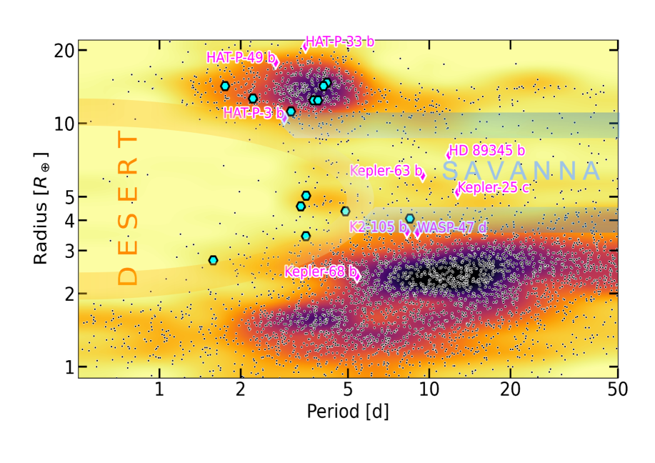
Figure 1: Two-dimensional distribution of exoplanets as a function of their radius and period from the NASA Exoplanet Archive (Akeson et al. 2013). Magenta and pink diamonds represent DREAM III and Allart et al. (2023) -a work that we took as a reference for our analysis- targets, respectively. The approximate boundaries of the desert and savanna are highlighted.

2 Sample

Our survey consists of nine planets along the transitions defining the Neptunian desert and savanna. Their low densities ($\rho_{\mathrm{pl}}$¡3.5 g cm^-3) and bright host stars (J¡10.7) favor observations of their atmosphere in the nIR. The planet and star parameters adopted in this work are presented in Table LABEL:Tab_parameters. Below, we describe the main features of interest for these planets, which led to their inclusion in our survey. We would like to stress that no helium studies were reported in the literature for these investigated planets.
Hot Jupiter HAT-P-3b. Its strong irradiation is expected to induce a large mass loss. The small radius of HAT-P-3b is indicative of a metal-enriched composition (Chan et al. 2011), which could be the result of atmospheric escape over the last 2.6 Gyr. Hydrogen would be lost preferentially, making helium a particularly interesting tracer for this planet. HAT-P-3b orbits a K-star, thus according to Oklopčić (2019), it is likely to show metastable helium absorption. DREAM I reports a polar orbit for this planet and, if confirmed, dynamical simulations will be needed to understand whether the present-day architecture is a result of a disruptive dynamical history (with partial evaporation of its volatile content) or a primordial misalignment between the protoplanetary disk and the star.
Hot Jupiter HAT-P-33b. The extreme irradiation and very low density (0.134${}_{-0.042}^{+0.053}$ g cm^-3, Wang et al. 2017) of this highly inflated planet are expected to induce a large mass loss. Turner et al. (2017) measured an excess depth during transit in the R-band, which contains the H$\alpha$ transition, suggesting that the planet may be undergoing hydrodynamical escape. The misalignment of the system, due to the inclination of the host star, suggests that HAT-P-33 b underwent a high-eccentricity migration, and thus it possibly migrated close to the star long after its formation, which would change its atmospheric history compared to an early-on migration and erosion.
Ultra-hot-Jupiter HAT-P-49b. It is a gas giant exoplanet discovered orbiting a bright (V = 10.3) slightly evolved F-star (Bieryla et al. 2014). Its extreme irradiation, due to its proximity to the host star (a=0.0438$\pm$0.0005 au, Bieryla et al. 2014), is expected to induce a large mass loss. According to the analysis presented in DREAM I, the planet is probably on a polar orbit, supporting a disruptive dynamical origin or evolution for the system, whose architecture was unaffected by tidal interactions with the shallow convective envelope of the host star (DREAM II).
Warm super-Neptune HD89345b. This planet is five times more irradiated than the evaporating super-Neptune WASP-107b, yet it survived atmospheric escape for 9.4 Gyr (e.g., Van Eylen et al. 2018). HD 89345b stands at the transition between stable Jupiter-mass planets and hot Neptunes that entirely lost their atmosphere and this is thus an essential piece in the puzzle that is the origin of the desert. HD 89345b is located on a misaligned orbit (DREAM I) right within the savanna (see Fig. 1). The present-day misalignment could trace both a primordial formation of the system, arising from the tilt of the early star or protoplanetary disk, or the planet could have migrated more recently, exiting a Kozai resonance with an outer companion (e.g., Bourrier et al. 2018; Attia et al. 2021). This second scenario would imply that HD 89345b arrived near the star at the end of its main-sequence lifetime, changing our view of its irradiative history and our interpretation of its inflation (Yu et al. 2018) and hydrodynamical escape.
Warm sub-Neptune K2-105b. It remains unclear why sub-Neptunes appear to be more resilient than warm Neptunes to the processes that created the desert (Owen 2019). K2-105b stands at the transition between these two populations and is predicted to have an atmosphere accounting for up to 10% of its total mass (Narita et al. 2017). Detecting the presence of this atmosphere and measuring its mass loss could bring constraints on the interior of the planet; if its evolution was controlled by atmospheric escape, it is estimated to have retained its envelope only if its core mass is greater than 6 M_⊕(Narita et al. 2017). DREAM I reported a possibly misaligned orbit which, if confirmed, might support a turbulent dynamical history and the planet’s late arrival into its close-in orbit. However, the presence of other targets may indicate a primordial inclination of the star or protoplanetary disk, as K2-105b is far away from its host stellar companion to experience tidal interactions.
Warm Neptune Kepler-25c. It is close to a resonant periodic configuration with a companion planet, which is known to be the final state of a system that undergoes migration within the protoplanetary disk (Migaszewski & Goździewski 2018). Kepler-25c should thus be evaporating since its formation 11 Gyr ago (Marcy et al. 2014), yet its low density (0.588${}^{+0.053}_{-0.061}$ g cm^-3, Mills et al. 2019) indicates the presence of a H/He envelope.
Warm Neptune Kepler-63b. It is a gas giant exoplanet with a radius between Neptune and Saturn. The orbital period is around 9.4 days, leading to an equilibrium temperature of about 900 K (Mallonn et al. 2022). The planet is in a polar orbit around a young Sun-like star (Sanchis-Ojeda et al. 2013, DREAM I), thus offering the possibility to assess how evaporation shapes a Neptune’s atmosphere in its early life. Its radius and insolation are similar to those of the other Neptunian targets, but it is much younger (200 Myr vs 10 Gyr) and still possibly undergoing vigorous escape.
Hot sub-Neptune Kepler-68b. With a density of 3.32${}^{+0.86}_{-0.98}$ g cm^-3(Gilliland et al. 2013), it is considered a candidate ocean planet (Zeng & Sasselov 2014) possibly topped by a moderate H/He envelope (Howe et al. 2014). Detecting He would offer insights on the mysterious nature of this sub-Neptune, representative of the transition between rocky planets and gas giants (Lopez & Fortney 2014).
Warm sub-Neptune WASP-47d. The WASP-47 planetary system is composed of at least four planets, a hot Jupiter (WASP-47 b; P = 4.159 days, Bryant & Bayliss 2022) with an inner super-Earth (WASP-47 e; P = 0.7896 days, Bryant & Bayliss 2022), a close-orbiting outer Neptune (WASP-47 d; P = 9.031 days, Bryant & Bayliss 2022), and a long-period giant planet (WASP-47 c; P = 588.4 days, Vanderburg et al. 2017; Bryant & Bayliss 2022). WASP-47 d is near a 2:1 resonance with the inner Hot Jupiter WASP-47b. It has a similar radius and insolation of K2-105b but is three times less massive. Their comparison could provide valuable insight into evaporation processes on sub-Neptunes.

3 Observations

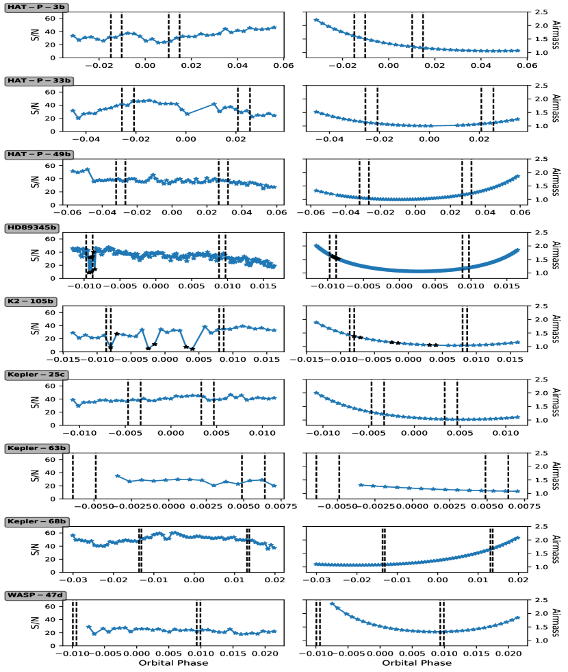
Figure 2: S/N in the region of interest (1082.2-1085.5 nm)(left panel) and airmass (right panel) measured during the GIARPS observations. The vertical dashed lines mark the $t_{1}$, $t_{2}$, $t_{3}$, and $t_{4}$ contact points (from left to right). Black stars indicate the discarded AB couples for low S/N.

Table 1: Log of TNG-GIANO-B observations.

Target	Night	S/NAVE	ammin-ammax	Nobs	Exposure time [s]
HAT-P-3b	2020-01-30	34	1.1-2.2	34	600.0
HAT-P-33b	2019-12-04	35	1.0-1.5	34	600.0
HAT-P-49b	2020-07-30	37	1.0-1.9	72	300.0+
HD89345b	2020-02-02	34	1.1-2.0	176	100.0
K2-105b	2020-01-18	27	1.0-1.9	32	600.0
Kepler-25c	2019-06-14	40	1.0-2.0	38	600.0
Kepler-63b	2020-05-13	27	1.1-1.3	14	600.0
Kepler-68b	2019-08-03	50	1.1-2.1	66	300.0
WASP-47d	2021-07-30	23	1.3-2.4	34	600.0

We observed the systems in our sample with the nIR echelle spectrograph GIANO-B installed on the 3.6 m Telescopio Nazionale Galileo (TNG) telescope. The observations were performed with the GIARPS configuration and were carried out with the nodding acquisition ABAB (Claudi et al. 2017). Therefore, while the targets were observed in one nodding position along the slit (A and B), the sky spectra were gathered simultaneously with the other one, thus providing an accurate reference for subtracting the thermal background and telluric emission lines.

GIANO-B covers the Y, J, H, and K spectral bands (0.95-2.45 $\mu$m) in 50 orders at a resolving power of R$\sim$50,000. For this analysis, we focus on order #39, where the helium triplet falls. We collected a transit observation for each investigated target. The only exception is HAT-P-3b, as due to bad weather conditions, we collected two nights of observation, namely UT 14 April 2019 and UT 30 January 2020, but the first visit was excluded from our analysis since observations had to be stopped just before the transit. A log of the observations is reported in Table 1. Figure 2 shows the variation in the signal-to-noise ratio (S/N) for order #39 and the variation in airmass for each exposure. Due to the lack of a sufficient number of collected images, we had to discard Kepler-63b from our analysis. Moreover, K2-105b’s and HD89345b’s observations were affected by GIANO-B auto-guide problems and by the presence of clouds, so we decided to discard the AB couples of exposures which exhibit a very low S/N.

4 Data analysis

Extended or evaporating atmospheres can be detected through an excess absorption by metastable helium in the planet transmission spectrum. In the following section, we discuss the steps we performed in order to reduce the raw GIANO-B data, extract individual transmission spectra, and calculate average in-transit spectra in the planet rest frame.

4.1 Initial data reduction

The raw spectra were dark-subtracted, flat-corrected, and extracted (without applying the blaze function correction) using the GOFIO pipeline (Rainer et al. 2018). In addition, GOFIO yields a preliminary wavelength calibration (defined in vacuum) using U-Ne lamp spectra as a template. We used the ms1d spectra, with the echelle orders separated and the Barycentric Earth Radial Velocity (BERV) correction applied, the spectra are defined in the terrestrial rest frame.

Since the U-Ne is acquired at the end of the night to avoid the persistence of the saturated signal of some emission lines on the detector polluting the scientific observations, the mechanical instability of GIANO-B makes the wavelength solution determined by GOFIO insufficient in terms of accuracy. We corrected for this by aligning all the GIANO-B spectra to the telluric reference frame via spline-interpolation based on the retrieved shifts obtained by cross-correlating with a time-averaged spectrum used as a template (Brogi et al. 2018; Guilluy et al. 2019, 2020; Giacobbe et al. 2021). We thus aligned the spectra to the reference frame of the Earth’s atmosphere, which is also assumed as the frame of the observer (neglecting any $\sim$10 m s^-1 differences due to winds). We then used the atmospheric transmission spectrum generated via the ESO Sky Model Calculator to refine the initial GOFIO wavelength calibration.

4.2 Transmission spectroscopy

We performed the transmission spectroscopy, applying the steps described below to each transit and target independently and considering the system parameters listed in Table LABEL:Tab_parameters.

4.2.1 Telluric correction

First, we performed a detailed correction for telluric contamination. We used the Molecfit ESO software (Smette et al. 2015; Kausch et al. 2015) to correct for the transmission telluric lines (Allart et al. 2017). As this is the first time that Molecfit has been applied to GIANO-B data, we report the adopted parameters in Table 5 .

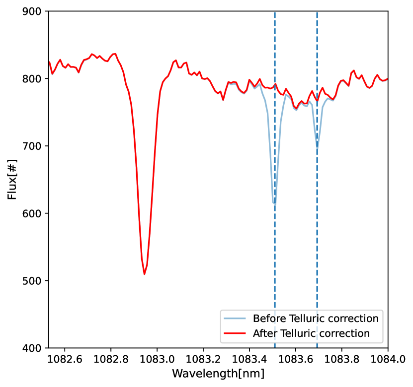
Figure 3: Example of a time-averaged spectrum before (in blue) and after the telluric lines removal (in red). Dashed vertical lines highlight the position of two H₂O telluric lines, i.e., 1083.51 nm and 1083.69 nm, in the region around the He I triplet. These two lines are corrected in the red spectrum.

Molecfit is based on a combination of two different sources: an atmospheric standard profile (MIPAS), and a Global Data Assimilation System (GDAS) profile. Molecfit gives the merging of these two profiles as input for a line-by-line radiative transfer model (LBLRTM). We considered the precipitable water vapor in our transmission model, and selected a fixed grid to merge the two atmospheric models, namely, the variations in temperature, pressure, humidity, and abundance of H₂O from 0 to 120 km are described with a fixed number of layers (50). Meanwhile, LBLRTM returns the telluric spectrum. We considered one observation at a time,and we initially performed the model fitting on selected spectral intervals inside the order #39 showing a well-determined continuum level, a good number of telluric lines, and a few or zero stellar lines. Based on the best-fit parameters derived by Molecfit, we then generated a telluric spectrum for the entire spectral order and we corrected the science spectrum. An example of telluric removal is shown in Fig. 3.

In the spectral region of interest, there are three OH emission lines that fall near the He I triplet (at $\sim$1083.21 nm, $\sim$1083.24 nm, and $\sim$1083.43 nm, vacuum wavelengths). As the observations were gathered with the nodding acquisition mode that allows for the subtraction of the thermal background and emission lines (see Sect. 4.1), there is no need to correct for telluric emission lines. However, due to seeing variations during the observing nights, the A-B subtraction can leave some residuals at the wavelengths of the OH lines. We thus masked the correspondent wavelengths.

4.2.2 Alignment into stellar rest frame.

We then shifted the spectra in the stellar rest frame by accounting for the stellar radial velocity, $V_{\star}$, in the telluric reference system. This is given by:

$$V_{\star/\oplus}=\sum_{i}{K_{\star i}[cos(\nu_{i}+\omega_{i})}+e_{i}cos(\omega_{i})]+V_{\mathrm{sys}}+V_{\mathrm{bar}},$$ (1)

where we account for the velocity of the observer induced by the rotation of the Earth and by the motion of the Earth around the Sun, namely: the barycentric Earth radial velocity, $V_{\mathrm{bar}}$, the stellar reflex motion induced on the host star by each planet $i$ in the system (i.e. $K_{\star i}[cos(\nu_{\mathrm{i}}+\omega_{\mathrm{i}})+e_{\mathrm{i}}cos(\omega_{\mathrm{i}})]$, where $\nu_{\mathrm{i}}$ is the true anomaly obtained from the eccentric anomaly via the Kepler’s equation, in this way we directly account for the eccentricity which is significative for some of our targets, e.g., HAT-P-33b, HD89345b), $\omega_{\mathrm{i}}$ is the argument of periastron, $e_{\mathrm{i}}$ is the eccentricity, and $K_{\star i}$ is the stellar radial-velocity semi-amplitude, and the systemic velocity of the star-planets system with respect to the barycentre of the Solar System ($V_{\mathrm{sys}}$).

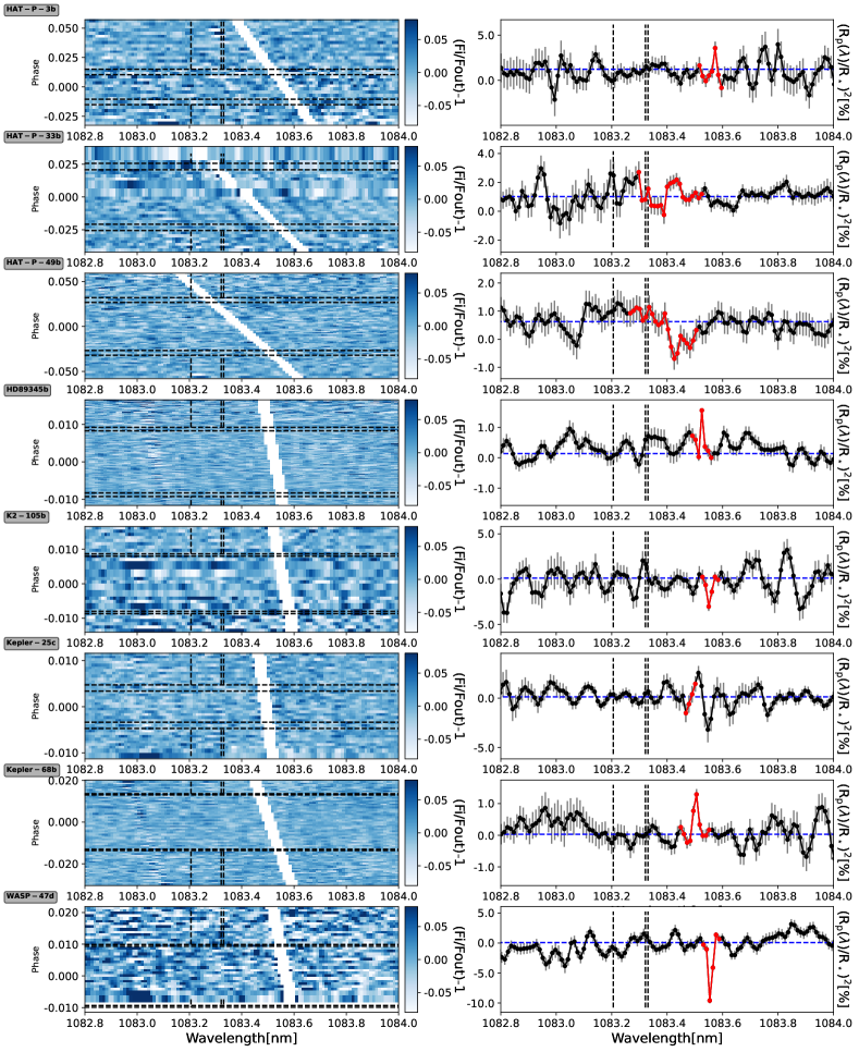
Figure 4: Transmission spectra (T_λ,i=$\tilde{\mathrm{F}_{\mathrm{i}}(\lambda)}$/S${}_{\mathrm{out}}(\lambda)$ -1) shown in tomography in the planetary rest frame in the region of the He I triplet, as a function of wavelength and planetary orbital phase (left). The contact points t₁, t₂, t₃, and t₄ are marked with horizontal black lines. The regions affected by OH^- contamination are masked. Mean-transmission spectrum for each observed transit (right). The horizontal blue line is the white-light radius $(R_{\mathrm{pl}}/R_{\star})^{2}$. The mean transmission spectra have an inverted sign compared to $\tilde{\mathrm{F}_{\mathrm{i}}(\lambda)}$/S${}_{\mathrm{out}}(\lambda)$ -1 as the radius is expressed instead of absorption. Black vertical lines indicate the position of the He I lines. Red line marks the spectral regions affected by OH^- emission. For some planets, some residuals are left at the position of the Si line ($\sim$1083 nm). This is due to the depth of the line which can give rise to difficulties in the spectral extraction (see e.g., Krishnamurthy et al. 2023)

.

4.2.3 Transmission spectra calculation.

For every considered target, we divided each spectrum by its median value, thus obtaining the normalized spectra, $\tilde{\mathrm{F}_{\mathrm{i}}}$. We then built a master stellar spectrum, $S_{\mathrm{out}}(\lambda)$, by averaging the out-of-transit spectra (i.e., with an orbital phase smaller than t₁ or greater than t₄), and derived individual transmission spectra, $T_{\mathrm{\lambda,i}}$, by dividing each spectrum by $S_{\mathrm{out}}(\lambda)$, that is, T_λ,i=$\tilde{\mathrm{F}_{\mathrm{i}}(\lambda)}$/S${}_{\mathrm{out}}(\lambda)$ -1. Finally, we linearly interpolated transmission spectra in the planet rest frame, as follows:

$$\begin{split}V_{\mathrm{pl_{j}/\star}}&=-\sum_{i}{K_{\star i}[cos(\nu_{i}+\omega_{i})+e_{i}cos(\omega_{i})]}\\ &-K_{\mathrm{pl_{j}}}(cos(\nu_{j}+\omega_{j})+e_{j}cos(\omega_{j})),\end{split}$$ (2)

where $K_{\mathrm{pl_{j}}}$ is the computed planet radial-velocity semi-amplitude (see Table LABEL:Tab_parameters) of the considered target $j$). The 2D maps of the transmission spectra in the planet rest frame are shown in the left panels of Fig. 4.

The usual method to search for faint planetary atmospheric signatures is to average in-transit transmission spectra in the planet rest frame and thus boost the S/N. However, the naive calculation of transmission spectra performed above neglects the change in broadband flux level of in-transit flux spectra, due to the occultation of regions with varying flux intensity by the opaque planetary disk. For example, limb-darkening, if unaccounted for, biases the retrieved atmospheric absorption signal toward smaller values at phases close to the stellar limb, as compared to the stellar disk center. We thus followed the approach presented in Mounzer et al. (2022) that had been re-adapted from Wyttenbach et al. (2020) to compute the in-transit transmission spectra:

$$\left(\frac{R_{\mathrm{pl}}(\lambda,t)}{R_{\star}}\right)^{2}=\frac{LD_{\mathrm{mean}}}{LD(t)}\frac{F_{\mathrm{out}}(\lambda)-(1-\delta(t))F_{\mathrm{i}}(\lambda,t)}{F_{\mathrm{local}}(\lambda,t)},$$ (3)

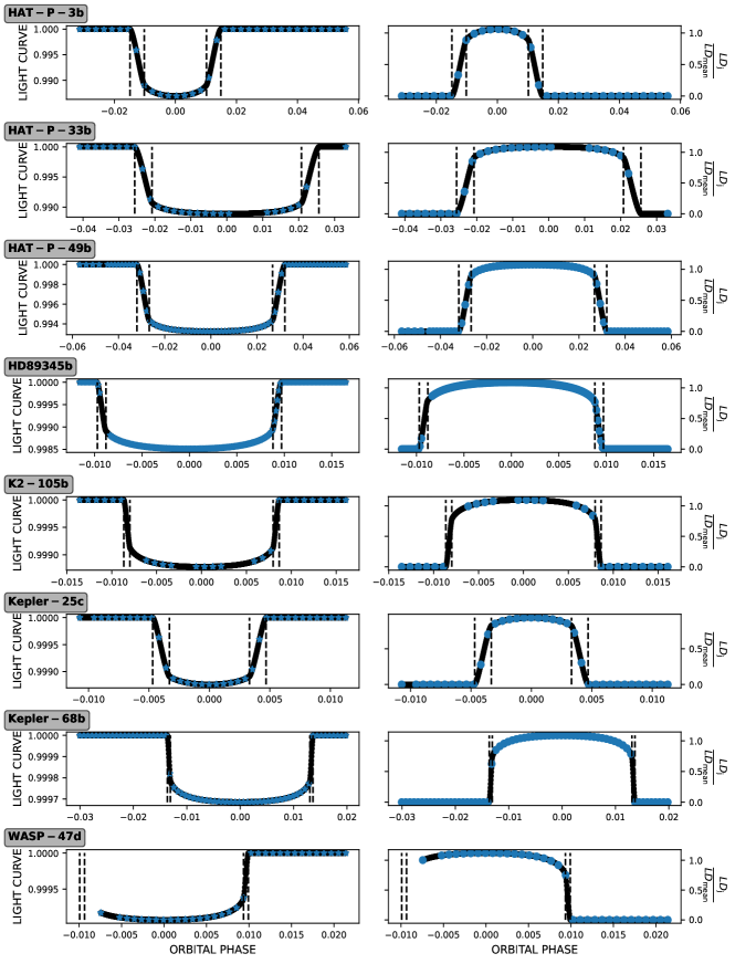
Figure 9: Light curves (left panels) and the limb-darkening ratio, namely, $\frac{LD_{\mathrm{j}}}{LD_{\mathrm{mean}}}$ with $j$ the orbital phase (right panels) computed with the Python $batman$ code (Kreidberg 2015) and the system parameters from Table LABEL:Tab_parameters. The contact points t₁, t₂, t₃, and t₄ are marked with vertical black lines. Blue dots are the light curves and limb-darkening ratio at the observed phases.

where $F_{\mathrm{i}}(\lambda,t)$ is each observed spectrum at phase $t$, $1-\delta(t)$ is the broadband (”white-light”) transit light curve, $\delta(t)$ is the transit depth, $LD(t)$ and $LD_{\mathrm{mean}}$ represent the stellar limb darkening at the position of the transiting planet and the disk-averaged limb-darkening, respectively. We used the Python $batman$ code (Kreidberg 2015) and the system parameters from Table LABEL:Tab_parameters to calculate the white-light transit light curve and the limb-darkening coefficients (see Fig. 9). $F_{\mathrm{local}}(\lambda)$ is the normalized local stellar spectrum (see Sect. 6) occulted by the planet at phase $t$. We applied Eq. 3 only to fully in-transit orbital phases (i.e., obtained between the t₂ and t₃ contact points), while ingress, and egress were not considered here. Indeed LD, and occulted stellar surface are not well known at the limbs. If we neglect the RM effect and center-to-limb (CLV) variations, the occulted local stellar spectrum $F_{\mathrm{local}}(\lambda)$ is equal to the disk-integrated stellar spectrum $F_{\mathrm{out}}(\lambda)$ (see Sect. 6), so that Eq. 3 becomes:

$$\left(\frac{R_{\mathrm{pl}}(\lambda,t)}{R_{\star}}\right)^{2}=\frac{LD_{\mathrm{mean}}}{LD(t)}\left(1-\frac{(1-\delta(t))F_{\mathrm{i}}(\lambda,t)}{F_{\mathrm{out}}(\lambda,t)}\right).$$ (4)

All transmission spectra fully in-transit were finally averaged (T_mean) to create one transmission spectrum for each observed transit (right panels of Fig. 4).

4.2.4 Fringing correction

Our GIANO-B spectra presented a sinusoidal fringing pattern caused by the sapphire substrate ($\sim$0.38 mm thick) placed above the sensitive part of the detector, which behaves as a Fabry-Pérot in generating interference fringing. Such fringing patterns must be corrected for in studying the He I triplet. We followed and re-adapted the second and third approaches (Method#1b-Method#2) presented in Guilluy et al. (2019). We focused on correcting this effect at the level of the final transmission spectra in order to have better control over fringing in the final transmission spectrum itself and to avoid risks in ”overfitting” the data. First, for each planet, we binned T_mean (bin size of 0.2 nm), we thus computed the Lomb-Scargle periodogram to find the characteristic frequency of the periodic fringing signal present in the data $f_{\mathrm{best}}$. We then selected the most prominent frequency of the periodogram, and we fitted the fringing pattern using a sine function $yfit=C+A\sin(2\pi\lambda f+\phi)$, where $A$ is the amplitude, $\phi$ the phase, $f$ is the fringing frequency (where we assumed $f_{\mathrm{best}}$ as starting point for the fit), and $C$ is the overall offset. We finally corrected our final transmission spectra by $yfit$.

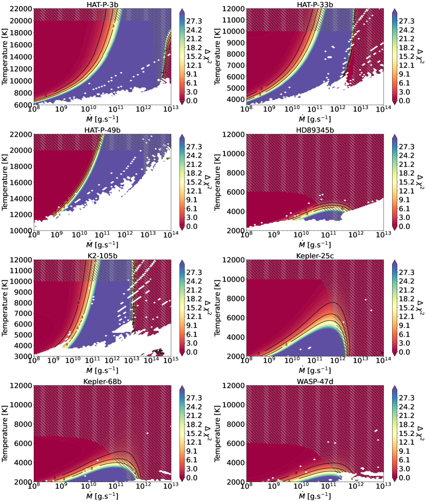
Figure 5: $\Delta\chi^{2}$ maps of mass-loss rate and temperature for the planets of our survey. Regions of the parameter space in red are consistent with the non-detections in our data, while models in purple are strongly disfavored. The thermospheric model failed to converge in white regions. Hatched regions are physically excluded.

5 Interpretation of the transmission spectra

Somewhat surprisingly no He I absorption signature was detected in our sample, as can be seen in Fig. 4. This either means that the targeted planets have no extended atmosphere, which would be surprising given the strong irradiation of their H/He atmosphere; or that their thermosphere’s metastable helium population is not dense enough to be detectable within the precision of the GIANO-B observations. Under this assumption, we can still put upper limits on the escape rate by fitting the transmission spectra with models of the planets’ thermospheric structure.

5.1 Stellar modelling

Given the scarcity of stellar high-energy measurements, we calculated the X-EUV spectral energy distribution of the eight target stars in a consistent manner using Table 5 in Linsky et al. 2014. This formula depends on the total X-EUV flux emitted by the star, which is calculated based on the stellar age and Equations 3 and 4 from Sanz-Forcada et al. 2011.

5.2 Thermosphere modelling

We used an approximate 1D model, the p-winds (Dos Santos et al. 2022) code, largely based on the formulations of Oklopčić & Hirata (2018) and Lampón et al. (2020), to calculate the thermospheric structure and resulting signature of the metastable helium triplet. The atmospheric density and velocity profiles were calculated according to the Parker wind approximation, assuming an isothermal planetary outflow (Parker 1958). We assumed for all targets an atmospheric composition of 90 % H and 10 % He (a good approximation of the Jupiter H/He ratio) and an input stellar X-EUV spectrum (calculated as explained in Section 5.1). The code calculates only the density profiles of hydrogen in its neutral and ionized states, as well as that of helium in its neutral, excited, and singly ionized states. The signature of interest is the metastable transition at 1083.3 nm of the helium excited level. A theoretical ideal spectrum is calculated at mid-transit without taking into account geometrical effects and inhomogeneities of the stellar surface. This absorption signature is compared to the observed mean transmission spectrum to estimate upper atmosphere characteristics such as temperature and the mass-loss rates.

Since there is no clear evidence of a helium signature, we quickly explored the input parameter space of the p-winds models by varying only the isothermal temperature profile, $T$, and the total atmospheric escape rate, $\dot{M}$, while all other input parameters are fixed. For instance, H/He ratio was not a fitting parameter. We expect that this can slightly change the derived values, but the conclusion would still remain the same. In our models, the radius at the top of the simulated atmosphere was set to the Roche lobe (Eggleton 1983). We note that the value chosen for this upper radius has not been discussed in previous studies using the p-winds code or similar codes (e.g., Oklopčić & Hirata 2018; Lampón et al. 2020; Dos Santos et al. 2022; Kirk et al. 2022), even though it directly controls the amount of helium that contributes to the theoretical absorption signature. The preferred approach in the literature seems to be increasing the radius until the neutral triplet helium density no longer contributes significantly to the absorption signal. Yet this is hardly compatible with the change in nature of the atmosphere beyond the Roche lobe, from a collisional thermosphere shaped by planetary gravity, which may (at first order) still be described by a 1D vertical structure, to an asymmetrical exosphere shaped by the stellar gravity, radiation, and wind. Our choice to set the upper model radius at the Roche lobe is based on the reasonable assumption that once helium atoms escape into the exosphere, they cannot be excited into their metastable state by collisions anymore and are quickly photo-ionized so that these layers contribute little to the observed signature (as supported by the lack of clear detection of extended exospheric tails in the literature).

In our simulations, high escape rates lead to an increase in the total density of metastable helium in the thermosphere but the densest layers are shifted to higher altitudes above the Roche lobe, where they no longer contribute to the theoretical signature. This boundary effect is visible in Fig. 5, with the reappearance of fit regions compatible with the non-detection of an absorption signature in our data. Simulations at high escape rates are therefore model-biased and should be considered cautiously. Furthermore, we note that the code p-winds was unable to calculate the atmospheric structure in certain regions of the parameter space (shown in white in Fig. 5). It is still unclear whether this is a numerical issue or a truly non-physical regime for the thermosphere.

5.3 Parameter space exploration

We determined whether the models were compatible with the measured transmission spectra using $\chi^{2}$ comparison. Since no absorption signature was detected for any of the planets we took the null hypothesis (a flat transmission spectrum) as the best-fit model and use $\Delta\chi^{2}=\chi^{2}_{model}-\chi^{2}_{flat}$ as a criterion to determine 3-$\sigma$ upper limits on the atmospheric mass-loss rate. We constrained the parameter space to realistic models in mass loss, using the maximum efficiency for a photoionization-driven isothermal Parker wind (Vissapragada et al. 2022), and in temperature, using the model of Salz et al. (2016) as a function of the gravitational potential of the planet. Below log($-\Phi_{G}$) = log $GM_{pl}/R_{pl}$ = 13.0 erg$\cdot$g^-1, their model predicts temperatures lower than 10 000 K, while above this limit, it predicts temperatures lower than 20 000 K. $\chi^{2}$ maps as a function of mass loss and temperature are shown in Fig. 5 for all planets in our sample. Table 10 gathers all the derived 3-$\sigma$ upper limits.

6 Accurate stellar line profiles

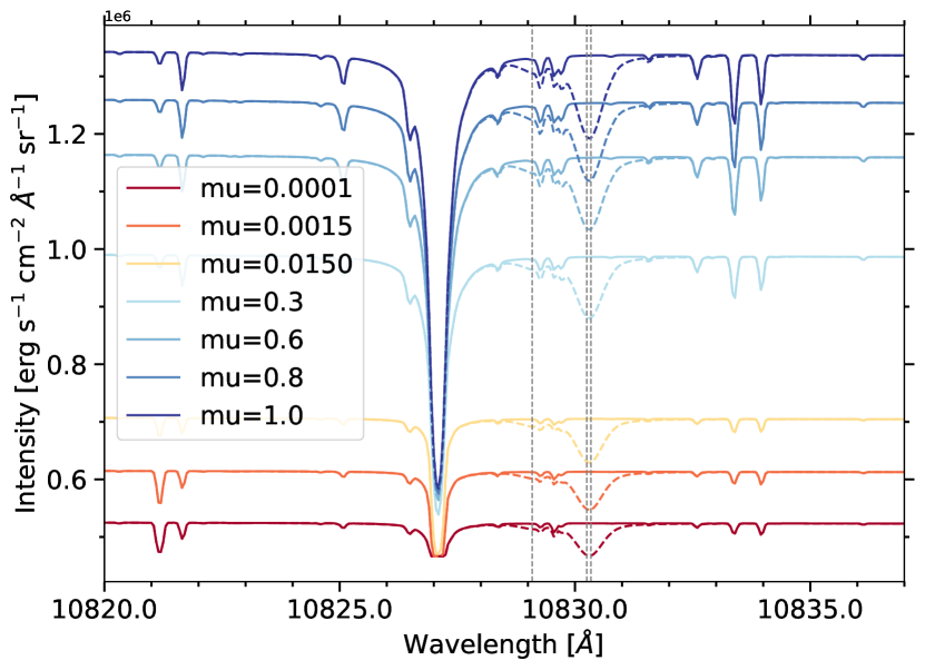
Figure 6: Spectral intensities for different $\mu$ positions on the stellar disk of HAT-P-33 derived with Turbospectrum. The dotted spectra are obtained after the multiplication of the intensity spectra by the He I triplet spectral profile. $\mu=\sqrt{1-(x^{2}+y^{2})}$ with $(x,y)$ the coordinates of a point on the stellar disk of radius equal to one in the Cartesian referential centered on the stellar disk.

Planet-occulted line distortions (POLD, Dethier & Bourrier 2023) can bias or even hide planetary absorption signatures in transmission spectra (Yan et al. 2017; Casasayas-Barris et al. 2020, 2021b). They appear in particular when one uses the disk-integrated stellar spectrum (F_out) to normalize the spectrum that is absorbed by the planet and its atmosphere. Indeed, the line profiles of F_out are shaped by a combination of the local effects of stellar rotation and CLV from all over the stellar disk; thus, they are not necessarily representative of the line profiles occulted by the planet. To mitigate the POLDs one needs to define more accurate estimates of the local stellar spectrum occulted by the planetary disk at each exposure. However, this quantity is complex to estimate from observations, as stars cannot be resolved spatially.

To estimate the planet-occulted stellar spectrum, we fit a model to the measured disk-integrated spectrum, using a combination of analytical and simulated theoretical local spectra. The stellar disk is discretized by a 2D uniform square grid, each cell being associated with a specific local intensity spectrum.

The simulated component of these intensity spectra is defined using the Turbospectrum code for spectral synthesis (Plez 2012). This code uses MARCS photospheric models (Gustafsson et al. 2008) and spectral line-lists from VALD3 database (Ryabchikova et al. 2015) to generate synthetic spectra under the assumption of local thermodynamic equilibrium. For each star, we used Turbospectrum to generate high-resolution intensity spectra for a series of positions along the stellar radius to sample broadband limb-darkening and CLV.
These synthetic spectra, however, do not contain the He I triplet lines at 10830Å  as its formation in stellar atmospheres necessitates non-local thermodynamical equilibrium conditions that are usually met in chromospheric layers, whereas MARCS models focus on the photospheric layers. We thus calculate the He I triplet absorption lines analytically, assuming Gaussian cross-sections and a common temperature and density for the metastable helium gas. Figure 6 shows a series of intensity spectra across the stellar disk of HAT-P-33.

The series of synthetic+analytical intensity spectra is then interpolated over the whole stellar grid, and Doppler-shifted according to the local radial velocity set by the projected stellar rotational velocity (Bourrier et al. 2023). Subsequently, intensity spectra are scaled into local flux spectra using the surface of the stellar grid cells, and summed over the whole grid to derive a simulated disk-integrated spectrum of the target star. Finally, the disk-integrated spectra are convolved with GIANO-B instrumental response and resampled to match its spectral resolution. The observed and simulated disk-integrated spectra are compared using a MCMC fit with free parameters set to the temperature and density of the metastable helium atoms.

Figure 7 shows the results of our fits for HAT-P-33 and HAT-P-49, which have the highest $v$sin$i_{\star}$ of our sample, highlighting the local spectrum at disk’s center that is later used in Eq. 3. We only applied this approach to the four targets with the highest $v$sin$i_{\star}$, as POLDs are expected to be negligible for the other targets. For these slow rotators, the rotational broadening of the disk-integrated line profiles is small and they remain good proxies for the local planet-occulted lines, especially for the shallow He I triplet lines. We note that CLV is not accounted for in our analytical estimates of the He I lines.

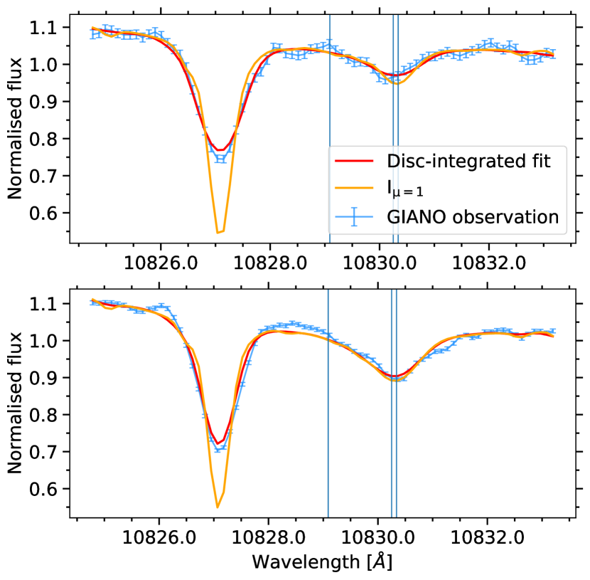
Figure 7: Normalized spectra of HAT-P-33 (upper panel) and HAT-P-49 (lower panel). We show the best fit (red curve) to the observed (blue curve) disk-integrated spectrum, and the spectrum at the disk’s center (orange curve). The blue vertical lines show the transition wavelength of the He I triplet.

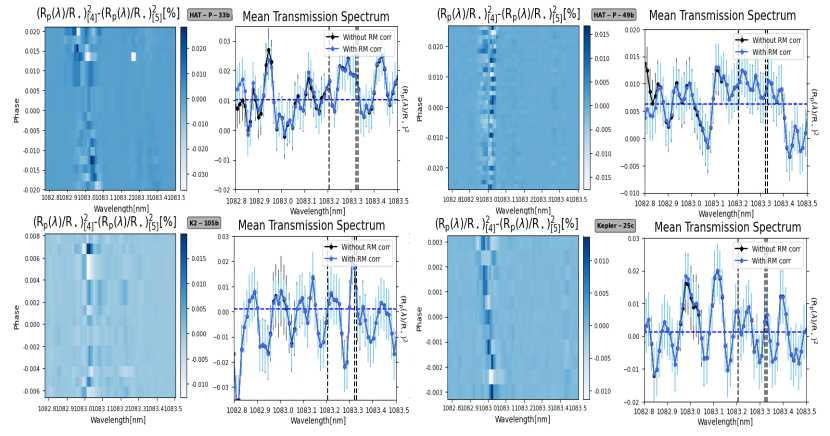
Figure 11: Difference between the full in-transit transmission spectra in stellar rest frame when both accounting and not accounting for the RM effects (left panel). Average full in-transit transmission spectrum in the planet rest frame when both accounting (blue line) and not accounting (black line) for the RM effect (right panel). Left panels also show the difference between the transmission spectra calculated with formula 3, with the RM correction, and 4, no RM correction applied, in the stellar rest frame. The RM signal creates a signature that is comparable to the dispersion in a given transmission spectrum and furthermore smoothes out when averaging over the transit because the RM signature shifts along the transit chord radial velocities.

We underline that even for the four fast-rotating targets for which we used a more accurate proxy for the planet-occulted stellar line the amplitude of the POLD was found to be comparable to the dispersion of the data. This is partly due to the shallowness of the He I triplet lines, and to the fact that POLDs partially smooth out when averaging transmission spectra in the planet rest frame over the transit window. Indeed, POLDs shift along the stellar surface RVs, while planetary signatures shift along the planet orbital RVs (see Fig. 11). Therefore, our final interpretation is made based on the transmission spectra calculated with the disk-integrated spectrum.

7 Results

Table 2: He I measurements.

Target	Roche lobe	gP	Excess of absorption	Heq	$\delta_{\mathrm{R_{P}}}$/Heq	F${}_{\mathrm{5-504\leavevmode\nobreak\ \textnormal{Å}}}$	$\dot{M}$ 3$\sigma$
	[RP]	[m s-2]	[$\%$]	[Km]		[103 erg s-1 cm-2]	[1010 g s-1]
HAT-P-3b	3.647	17.5	¡ 1.9	424	92	7.968	7.772
HAT-P-33b	2.167	5.1	¡ 1.4	2231	33	6.195	8.205
HAT-P-49b	3.207	21.5	¡ 0.6	629	61	14.51	5.702
HD89345b	8.213	7.8	¡ 0.7	855	76	0.244	3.899
K2-105b	11.202	23.6	¡ 2.33	219	378	14.69	6.028
Kepler-25c	8.148	5.3	¡ 1.86	1192	82	1.019	65.26
Kepler-68b	8.722	15.2	¡ 0.72	533	112	1.176	8.134
WASP-47d	9.565	10.9	¡ 3.29	533	230	0.577	7.854

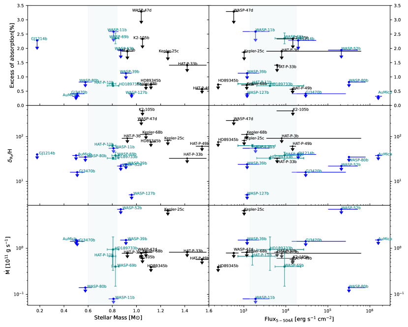
Figure 8: Correlation plots. Excess of absorption (top panels), $\delta_{\mathrm{R_{P}}}$/H_eq (middle panels) and mass-loss rates (bottom panels) as a function of stellar mass and XUV irradiation at the planet position. Upper limits are given at 3$\sigma$. Blue stars are targets reported from Allart et al. (2023), the detections and the non-detections are plotted in dark- and light-blue, respectively. We note that K2-105 b observations suffered from GIANO-B’s auto-guide problems and low S/N, so the limit we set on $\delta_{\mathrm{R_{P}}}/H_{\mathrm{eq}}$ is not constraining. We highlighted in gray the area of the parameter space that accordingly to Allart et al. (2023) seems to favor the detections. The errors on the XUV flux have been calculated with the error on the stellar ages.

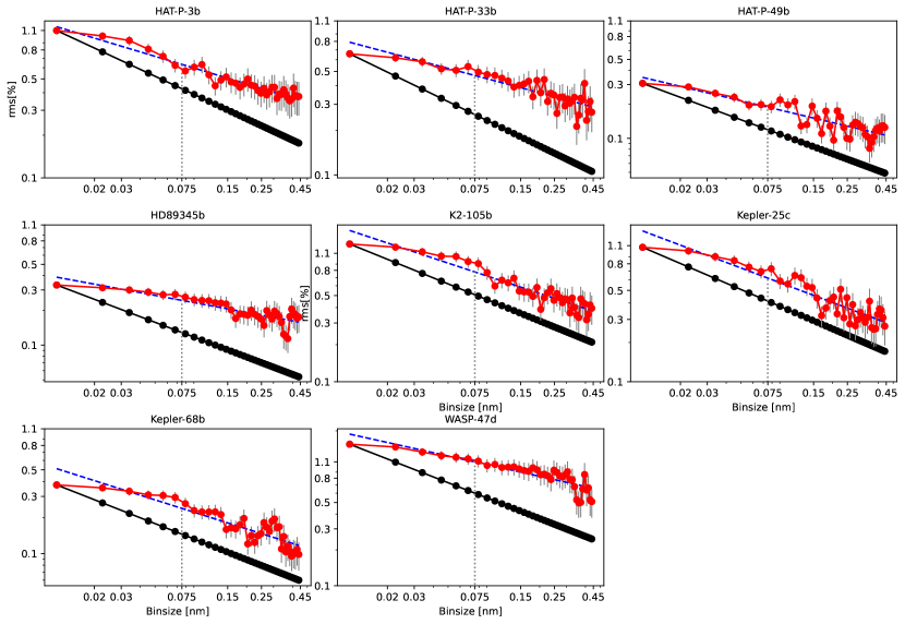
Figure 12: Allan plot computed on the average transmission spectra. The back lines are the expected rms for white noise (which scales with the number of points for bin). The red dotted curves are the standard deviation of the transmission spectrum after various binning of different bin size. The dashed blue lines are the best fit for the red curves (computed in log-log scale). The vertical gray lines are the derived 1$\sigma$ uncertainty at 0.075 nm. The error bars denote this 1$\sigma$uncertainty of the rms (Cubillos et al. 2017).

The presence of an extended and possibly escaping helium atmosphere would appear as an absorption feature in the transmission spectrum in the planet’s rest frame at the position of the stellar helium triplet. Unfortunately, as shown in Fig. 4, we did not detect significant helium absorption features for any of our targets. We thus evaluated 3$\sigma$ upper limits from the data itself as in Allart et al. (2023). Following an approach similar to that of Cubillos et al. (2017), we computed Allan plots (see Fig. 12) to estimate the noise present in the data. We assumed the white noise $\sigma_{1}$ to be the standard deviation (hereafter, root mean square, rms) of the transmission spectrum, excluding the helium triplet region (1083.0-1083.6 nm). Then, we binned the transmission spectrum by bins of $N$ elements each and calculated the rms of the binned transmission spectrum. We repeat the process for a wide range of $N$ elements for bin (from 1 to 42). In the absence of correlated noise, $\sigma_{1}$ scales as $\sqrt{N}$. We then fitted the rms in a log-log space to derive the trend of the noise, the fitted rms at 0.075 nm is the 1 $\sigma$ uncertainty. We set three times this value as the 3$\sigma$ upper limit on the signature contrast, $c$.
An alternative approach to providing more rigorous estimations of the noise present in the data requires the use of Gaussian processes (See Appendix Sect. B). However, for the rest of the analysis, to maintain consistency with the results published in Allart et al. (2023), we used upper limits estimated from Allan plots.
We then derived an upper limit on the equivalent opaque radius $\delta_{\mathrm{R_{P}}}$, namely, the height of an opaque atmospheric layer that would produce the observed absorption signal, as:

$$\delta_{\mathrm{R_{P}}}=\sqrt{(R_{\mathrm{P}}^{2}+R_{\mathrm{\star}}^{2}\times c)}-R_{\mathrm{P}}\,,$$ (5)

where $R_{\mathrm{p}}$ and ${R_{\star}}$ are the planetary and stellar radius, respectively.
We finally computed the quantity $\delta_{\mathrm{R_{P}}}/H_{\mathrm{eq}}$ (Nortmann et al. 2018), which expresses the number of scale heights ($H_{\mathrm{eq}}$) probed by the atmosphere in the considered spectral range, with $H_{\mathrm{eq}}$ = $\frac{k_{\mathrm{B}}T\mathrm{eq}}{\mu g}$ and $k_{\mathrm{B}}$ the Boltzmann constant, $T_{\mathrm{eq}}$ the planetary equilibrium temperature (listed in Table LABEL:Tab_parameters), $g$ the planetary gravity computed from the planetary mass and radius (reported in Table 10), $\mu$ the mean molecular weight (for which we assumed a hydrogen-dominated atmosphere and hence a value of 1.3 times the mass of a hydrogen atom). Table 10 reports the derived $\delta_{\mathrm{R_{P}}}/H_{\mathrm{eq}}$ values for each investigated planet.

We explored how the derived constraints vary as a function of the stellar mass and XUV flux between 5 and 504 Å, which are the energies mainly responsible for the population of the metastable He I level (Sanz-Forcada et al. 2011). We focused on these two parameters because Allart et al. (2023) showed that they do yield visible trends with $\delta_{\mathrm{R_{P}}}/H_{\mathrm{eq}}$. Trends related to the excess of absorption and atmospheric extension are shown in the top and middle panels of Fig. 8. All our targets are outside the area of the parameter space, with masses between $\sim$0.6 and $\sim$0.85 M_⊙, as pointed out by Allart et al. (2023) to favor the He I detection. This range of stellar masses corresponds to K-stars, in agreement with the predictions of Oklopčić (2019), thus our non-detections are not entirely unexpected. However, half of our non-detections do not agree with the XUV flux range found to favor the presence of He I in Allart et al. (2023), 1400-17800 erg s${}^{-1}\,$cm^-2. However, the XUV flux values depend on the model and are associated with star ages, which are typically not well-constrained. So we have to be cautious with these values. Finally, as already highlighted in Allart et al. (2023), even if surprising, there are no clear correlations between Ṁ and the stellar mass or XUV flux (bottom panels of Fig. 8).

We chose to focus on the targets analyzed in this paper and in Allart et al. (2023), rather than other results from the literature because we derived the absorption, atmospheric extension, and mass-loss values homogeneously with the same methodology.

8 Summary and conclusions

In this paper, we describe our He I survey of 9 planets at the edge of the Neptunian desert, with the goal of understanding the role of photoevaporation in sculpturing this feature. We analyzed observations gathered with the high-resolution GIANO-B spectrograph mounted on the TNG, and we used the transmission spectroscopy technique to detect a possible extended or evaporating helium atmosphere in the investigated planets. We found no sign of planetary absorption at the position of the stellar He I triplet in any of the investigated targets, and we thus provided 3$\sigma$ upper limits on the He I absorption. We underline that the GIANO-B transmission spectra are affected by various systematics that are not fully understood and difficult to properly remove. These systematics may be caused by low data quality (e.g., low S/N) or instrumental effects (e.g., auto-guide problems).

We interpreted our derived transmission spectra with the p-wind code (Dos Santos et al. 2022) and we attempted to interpret our findings by putting them in the wider context of the measurements presented in Allart et al. 2023 submitted. We searched for correlations with the stellar mass and XUV flux (e.g., Fossati et al. 2022), which are thought to be key drivers in the formation of the He I triplet. Constraints from our sample support the trend of $\delta_{\mathrm{R_{P}}}/H_{\mathrm{eq}}$, with the stellar mass proposed by Allart et al. (2023), which remains a good indicator for the presence of metastable helium in exoplanet atmospheres. In addition, they are not incompatible with the trend highlighted in Allart et al. (2023) with the XUV flux as they are not constraining enough to reach a better precision. We stress the importance of carrying out helium surveys with the same instrument and analyzing them with the same data reduction technique, as heterogeneity can obscure any trends in the data (Vissapragada et al. 2022). Several instruments are now available to perform this kind of homogeneous survey such as NIRSPEC, SPIROU, CARMENES, and GIANO-B.

Appendix A Additional figures and tables

Table 3: Planets with He I study reported in the literature.

Planet	Status	Reference
WASP-11b	✗	Allart et al. 2023
WASP-12b	✗	Kreidberg & Oklopčić 2018
WASP-39b	✗	Allart et al. 2023
WASP-48b	✗	Bennett et al. 2023
WASP-52b	$\sim$	Vissapragada et al. 2020; Kirk et al. 2022; Allart et al. 2023
WASP-69b	✓	Nortmann et al. 2018; Vissapragada et al. 2020; Allart et al. 2023
WASP-80b	✗	Fossati et al. 2022; Vissapragada et al. 2022; Allart et al. 2023
WASP-76b	✗	Casasayas-Barris et al. 2021a
WASP-107b	✓	Spake et al. 2018; Allart et al. 2019; Kirk et al. 2020
WASP-127b	✗	dos Santos et al. 2020a; Allart et al. 2023
WASP-177b	✗	Kirk et al. 2022; Vissapragada et al. 2022
HD189733b	✓	Salz et al. 2018; Guilluy et al. 2020; Zhang et al. 2022a; Allart et al. 2023
HD209458b	$\sim$	Nortmann et al. 2018; Alonso-Floriano et al. 2019
HD97658b	✗	Kasper et al. 2020
HD63433b	✗	Zhang et al. 2022b
HD63433c	✗	Zhang et al. 2022b
HAT-P-11b	✓	Allart et al. 2018; Mansfield et al. 2018; Allart et al. 2023
HAT-P-18b	✓	Paragas et al. 2021; Vissapragada et al. 2022
HAT-P-26b	✓	Vissapragada et al. 2022
HAT-P-32b	✓	Czesla et al. 2022
NGTS-5b	$\sim$	Vissapragada et al. 2022
55Cnce	✗	Zhang et al. 2021
Kelt-9b	✗	Nortmann et al. 2018
GJ3470b	$\sim$	Ninan et al. 2020; Allart et al. 2023; Palle et al. 2020
GJ436b	✗	Nortmann et al. 2018
GJ1214b	$\sim$	e.g.,Orell-Miquel et al. 2022; Kasper et al. 2020; Allart et al. 2023
GJ9827b	✗	Carleo et al. 2021; Krishnamurthy et al. 2023
GJ9827d	✗	Kasper et al. 2020; Carleo et al. 2021; Krishnamurthy et al. 2023
TOI-560b	✓	Zhang et al. 2022a, 2023
TOI-1728b	✗	Kanodia et al. 2020
TOI-1430b	✓	Zhang et al. 2023
TOI-1683b	✓	Zhang et al. 2023
TOI-1807b	✗	Gaidos et al. 2023
TOI-2076b	✗	Zhang et al. 2023; Gaidos et al. 2023
TOI-3757b	✗	Kanodia et al. 2022
TOI-1235b	✗	Krishnamurthy et al. 2023
TOI-2136b	✗	Kawauchi et al. 2022
Trappist-1b	✗	Krishnamurthy et al. 2021
Trappist-1e	✗	Krishnamurthy et al. 2021
Trappist-1f	✗	Krishnamurthy et al. 2021
V1298Taub	$\sim$	e.g., Vissapragada et al. 2021; Gaidos et al. 2022
V1298Tauc	✗	e.g., Vissapragada et al. 2021
V1298Taud	✓	e.g., Vissapragada et al. 2021
AU Mic b	✗	Hirano et al. 2020
K2-25b	✗	Gaidos et al. 2020b
K2-100b	✗	Gaidos et al. 2020a

Table 4: Adopted parameters

Parameter	Value	Reference
HAT-P-3
$\bullet$ Stellar parameters
Spectral type	K1	Grieves et al. (2018)
Stellar mass, M⋆ (M⊙)	0.925 $\pm$ 0.046	Mancini et al. (2018)
Stellar radius, R⋆ (M⊙)	0.850 $\pm$ 0.021	Mancini et al. (2018)
Stellar age, $\tau$ (Gyr)	$2.9^{+2.7}_{-4.9}$	Mancini et al. (2018)
Effective temperature, Teff (K)	5190 $\pm$ 80	Mancini et al. (2018)
Metallicity (dex)	0.24 $\pm$ 0.08 (Fe/H)	Mancini et al. (2018)
log g (log10(cm s-2))	4.545 $\pm$ 0.023	Mancini et al. (2018)
Systemic velocity, vsys (km s-1)	-23.379680	DREAM I
Limb-darkening coefficients $\mu_{1}$	0.216	EXOFAST
$\mu_{2}$	0.286	EXOFAST
Stellar projected velocity, $v$sin$i_{\star}$ (km s-1)	$0.46^{+0.22}_{-0.25}$	DREAM 1
Magnitude (J-band)	9.936$\pm$0.022	Cutri et al. (2003)
$\bullet$ Planetary parameters
Orbital period, P (days)	2.89973797 $\pm$ 0.00000038	Baluev et al. (2019)
Transit epoch, T0 (BJDTDB)	2454218.75960 $\pm$ 0.00016	DREAM I
Eccentricity, e	0.0 (fixed)	Mancini et al. (2018)
Argument of periastron, $\omega_{\star}$	90 (fixed)	Mancini et al. (2018)
Stellar reflex velocity, K⋆ (m s-1)	90.63 $\pm$ 0.58	Mancini et al. (2018)
Scaled separation, a/R⋆	9.8105 $\pm$ 0.2667	Mancini et al. (2018)
Orbital inclination, $i$	86.31 $\pm$ 0.19 deg	Mancini et al. (2018)
Planet-to-star radius ratio, RP/R⋆	0.11091 $\pm$ 0.00048	Baluev et al. (2019)
Planetary mass, Mpl (Mjup)	0.595 $\pm$0.019	Mancini et al. (2018)
Planetary density, $\rho_{\mathrm{pl}}$ (g cm-3)	0.9750$\pm$0.1000	Mancini et al. (2018)
Projected spin-orbit angle, $\lambda$ (deg)	-25.3${}^{+29.4}_{-22.8}$	DREAM I
Planet radial-velocity semi-amplitude, Kpl(km s-1)	145.2$\pm$2.4	This paper
Equilibrium temperature, Teq(K)	1170$\pm$17	Mancini et al. (2018)
HAT-P-33
$\bullet$ Stellar parameters
Spectral type	F4	Luo et al. (2018)
Stellar mass, M⋆ (M⊙)	1.42 ${}^{+0.16}_{-0.15}$	Wang et al. (2017)
Stellar radius, R⋆ (M⊙)	1.91${}^{+0.26}_{-0.20}$	Wang et al. (2017)
Stellar age, $\tau$ (Gyr)	2.30 $\pm$ 0.30	Bonomo et al. (2017)
Effective temperature, teff (K)	6460 ${}^{+300}_{-290}$	Wang et al. (2017)
Metallicity (dex)	0.01 $\pm$ 0.31 [Fe/H]	Wang et al. (2017)
Surface gravity, log g⋆ (cgs)	$4.030_{-0.090}^{+0.079}$	Wang et al. (2017)
Systemic velocity, vsys (km s-1)	23.080601	DREAM I
Limb-darkening coefficients $\mu_{1}$	0.097	EXOFAST
$\mu_{2}$	0.301	EXOFAST
Stellar projected velocity, $v$sin$i_{\star}$ (km s-1)	15.57 $\pm$ 0.31	DREAM I
Magnitude (J-band)	10.263$\pm$0.021	Cutri et al. (2003)
$\bullet$ Planetary parameters
Orbital period, P (days)	3.47447773 $\pm$ 0.00000066	DREAM I
Transit epoch, T0 (BJDTDB)	2456684.86508 $\pm$ 0.00027	DREAM I
Eccentricity, e	0.180 ${}_{-0.096}^{+0.110}$	DREAM I
Argument of periastron, $\omega_{\star}$ (deg)	88${}^{+33}_{-34}$	Wang et al. (2017)
Stellar reflex velocity, K⋆ m s-1	74.4$\pm$8.5	DREAM I
Scaled separation, a/R⋆	5.69${}^{+0.58}_{-0.59}$	Wang et al. (2017)
Orbital inclination, $i$ (deg)	88.2 ${}^{+1.2}_{-1.3}$	Wang et al. (2017)
Planet-to-star radius ratio, RP/R⋆	0.10097 ${}^{+0.00056}_{-0.00052}$	Wang et al. (2017)
Planetary mass, Mpl (Mjup)	0.72 ${}^{+0.13}_{-0.12}$	Wang et al. (2017)
Planetary density, $\rho_{\mathrm{pl}}$ (g cm-3)	0.134${}_{-0.042}^{+0.053}$	Wang et al. (2017)
Projected spin-orbit angle, $\lambda$ (deg)	5.9$\pm$4.1 deg	DREAM I
Planet radial velocity semi-amplitude, Kpl(km s-1)	160.6${}^{+6.9}_{-6.3}$	This paper
Equilibrium temperature, Teq(K)	1782$\pm$28	Hartman et al. (2011)
HAT-P-49
$\bullet$ Stellar parameters
Spectral type	F3	DREAM I
Stellar mass, M⋆ (M⊙)	1.543$\pm$0.051	Bieryla et al. (2014)
Stellar radius, R⋆ (R⊙)	$1.833{+0.138}_{-0.076}$	Bieryla et al. (2014)
Stellar age $\tau$ (Gyr)	1.50 $\pm$ 0.20	Bonomo et al. (2017)
Effective temperature, Teff (K)	6820$\pm$52	Bieryla et al. (2014)
Metallicity (dex)	0.074$\pm$0.080 [Fe/H]	Bieryla et al. (2014)
Surface gravity, log g⋆ (cgs)	4.10$\pm$0.04	Bieryla et al. (2014)
Systemic velocity, vsys (km s-1)	14.208478	DREAM I
Limb-darkening coeffcients $\mu_{1}$	0.078	EXOFAST
$\mu_{2}$	0.303	EXOFAST
Stellar projected velocity, $v$sin$i_{\star}$ (km s-1)	10.68${}^{+0.46}_{-0.47}$	DREAM I
Magnitude (J-band)	9.550$\pm$0.020	Cutri et al. (2003)
$\bullet$ Planetary parameters
Orbital period, P (days)	2.6915539$\pm$0.0000012	DREAM I
Transit epoch, T0 (BJDTDB) (BJDTDB)	2456975.61736 $\pm$0.00050	DREAM I
Eccentricity, e	0.0 (fixed)	Bieryla et al. (2014)
Argument of periastron, $\omega_{\star}$ (deg)	90 (fixed)	Bieryla et al. (2014)
Stellar reflex velocity, K⋆ (m s-1)	177.6 $\pm$ 16.0	DREAM I
Scaled separation, a/R⋆	5.13 ${}^{+0.19}_{-0.30}$	Bieryla et al. (2014)
Orbital inclination, $i$ (deg)	86.2$\pm$1.7	Bieryla et al. (2014)
Planet-to-star radius ratio, RP/R⋆	0.0792 $\pm$ 0.0019	Bieryla et al. (2014)
Planetary Mpl (Mjup)	1.730 $\pm$ 0.205	Bieryla et al. (2014)
Planetary density, $\rho_{\mathrm{pl}}$ (g cm-3)	0.75$\pm$0.17	Bieryla et al. (2014)
Projected spin-orbit angle, $\lambda$ (deg)	-97.7$\pm$1.8	DREAM I
Planet radial velocity semi-amplitude, Kpl(km s-1)	176.5$\pm$2.0	This paper
Equilibrium temperature, Teq(K)	2131${}^{+69}_{-42}$	Bieryla et al. (2014)
HD89345
$\bullet$ Stellar parameters
Spectral type	G5	Cannon & Pickering (1993)
Stellar mass, M⋆ (M⊙)	1.120${}^{+0.040}_{-0.010}$	Van Eylen et al. (2018)
Stellar radius, R⋆ (R⊙)	1.657${}^{+0.020}_{-0.004}$	Van Eylen et al. (2018)
Stellar age, $\tau$ (Gyr)	9.40 ${}^{+0.40}_{-1.30}$	Van Eylen et al. (2018)
Effective temperature, Teff (K)	5499 $\pm$ 73	Van Eylen et al. (2018)
Metallicity (dex)	0.45$\pm$ 0.04 [Fe/H]	Van Eylen et al. (2018)
Surface gravity log g⋆ (log10(cm s-2))	4.044${}^{+0.006}_{-0.004}$	Van Eylen et al. (2018)
Systemic velocity, vsys (km s-1)	2.223394	DREAM I
Limb-darkening coeffcients $\mu_{1}$	0.182	EXOFAST
$\mu_{2}$	0.300	EXOFAST
Stellar projected velocity, $v$sin$i_{\star}$ (km s-1)	0.58$\pm$0.28	DREAM I
Magnitude (J-band)	8.091 $\pm$0.020	Cutri et al. (2003)
$\bullet$ Planetary parameters
Orbital period, P (Days)	11.8144024 $\pm$0.0000066	DREAM I
Transit epoch T0 (BJDTDB)	2458740.81147$\pm$0.00044	DREAM I
Eccentricity, e	0.208 $\pm$ 0.039	DREAM I
Argument of periastron $\omega$ (deg)	21.7 $\pm$ 19.1	DREAM I
Stellar reflex velocity, K⋆ (m s-1)	9.1 $\pm$ 0.5	DREAM I
Scaled separation, a/R⋆	13.625 $\pm$ 0.027	Van Eylen et al. (2018)
Orbital inclination, $i$ (deg)	87.68 $\pm$ 0.10	DREAM I
Planet-to-star radius ratio, RP/R⋆	0.03696 $\pm$ 0.00041	DREAM I
Planetary mass, Mpl (Mjup)	0.112$\pm$0.010	Van Eylen et al. (2018)
Planetary density, $\rho_{\mathrm{pl}}$ (g cm-3)	0.609$\pm$0.067	Van Eylen et al. (2018)
Projected spin-orbit angle, $\lambda$ (deg)	74.2${}^{+33.6}_{-32.5}$	DREAM 1
Planet radial velocity semi-amplitude, Kpl(km s-1)	99.2${}^{+1.4}_{-0.9}$	This paper
Equilibrium temperature, Teq(K)	1053$\pm$14	Van Eylen et al. (2018)
K2-105
$\bullet$ Stellar parameters
Spectral type	G5	This paper
Stellar mass, M⋆ (M⊙)	1.05 $\pm$ 0.02	Castro-González et al. (2022)
Stellar radius, R⋆ (R⊙)	0.97 $\pm$ 0.01	Castro-González et al. (2022)
Stellar age, $\tau$ (Gyr)	¿0.6	Narita et al. (2017)
Effective temperature, Teff (K)	5636${}^{+49}_{-52}$	Castro-González et al. (2022)
Metallicity (dex)	0.23${}^{+0.04}_{-0.03}$ [Fe/H]	Castro-González et al. (2022)
Surface gravity log g⋆ (log10(cm s-2))	4.49 $\pm$ 0.01	Castro-González et al. (2022)
Systemic velocity, vsys (km s-1)	-32.390637	DREAM I
Limb-darkening coefficients $\mu_{1}$	0.169	EXOFAST
$\mu_{2}$	0.299	EXOFAST
Stellar projected velocity, $v$sin$i_{\star}$ (km s-1)	2.13${}^{+0.96}_{-0.92}$	DREAM I
Magnitude (J-band)	10.541$\pm$0.02	Cutri et al. (2003)
$\bullet$ Planetary parameters
Orbital period, P (days)	8.2669897$\pm$0.0000057	DREAM I
Transit epoch, T0 (BJDTDB)	2458363.2387${}^{+0.00069}_{-0.000633}$	DREAM I
Eccentricity, e	0 (fixed)	DREAM I
Argument of periastron, $\omega$ (deg)	90 (fixed)	DREAM I
Stellar reflex velocity, K⋆ (m s-1)	9.4 $\pm$ 5.8	Narita et al. (2017)
Scaled separation, a/R⋆	17.39 $\pm$ 0.19	DREAM I
Orbital inclination, $i$ (deg)	88.62 $\pm$ 0.10	DREAM I
Planet-to-star radius ratio, RP/R⋆	0.03332 $\pm$ 0.00067	DREAM I
Planetary mass, Mpl (Mjup)	0.094 $\pm$ 0.060	Narita et al. (2017)
Planetary density, $\rho_{\mathrm{pl}}$ (g cm-3)	2.3${}^{+1.7}_{-1.6}$	This paper
Projected spin-orbit angle, (deg) $\lambda$	-81${}^{+50}_{-47}$	DREAM I
Planet radial-velocity semi-amplitude, Kpl(km s-1)	107.0$\pm$0.7	This paper
Equilibrium temperature, Teq(K)	814$\pm$12	Livingston et al. (2018)
Kepler-25
$\bullet$ Stellar Parameters
Spectral type	F8	DREAM I
Stellar mass, M⋆ (M⊙)	1.26 $\pm$ 0.03	Benomar et al. (2014)
Stellar radius, R⋆ (R⊙)	1.34$\pm$0.01	Benomar et al. (2014)
Stellar age, $\tau$ (Gyr)	2.75 $\pm$ 0.30	Benomar et al. (2014)
Effective temperature, Teff (K)	6354$\pm$27	Benomar et al. (2014)
Metallicity [Fe/H] (dex)	0.11$\pm$0.03	Benomar et al. (2014)
Surface gravity log g (log10(cm s-2))	4.285$\pm$0.003	Benomar et al. (2014)
Systemic velocity, vsys (km s-1)	-8.633258	DREAM I
Limb-darkening coeffcients $\mu_{1}$	0.106	EXOFAST
$\mu_{2}$	0.304	EXOFAST
Stellar projected velocity, $v$sin$i_{\star}$ (km s-1)	8.89${}^{+0.59}_{-0.63}$	DREAM I
$\bullet$ Planetary parameters
Magnitude (J-band)	9.764 $\pm$0.020	Cutri et al. (2003)
$\star$ Planet, $b$
Orbital period, P (days)	6.2385347882	Battley et al. (2021)
Transit epoch, T0 (BJDTDB)	2458648.00807${}^{+0.00057}_{-0.00051}$	DREAM I
Eccentricity, e	0.0029 ${}^{0.0023}_{-0.0017}$	Mills et al. (2019)
$\sqrt{e}\,\cos{\omega}$	0.042 ${}^{0.017}_{-0.036}$	Mills et al. (2019)
$\sqrt{e}\,\sin{\omega}$	0.007 ${}^{0.038}_{-0.035}$	Mills et al. (2019)
Stellar reflex velocity K⋆ (m s-1)	2.6$\pm$0.7	This paper
Orbital inclination $i$ (deg)	87.173${}^{0.084}_{-0.083}$	Mills et al. (2019)
Planet-to-star radius ratio RP/R⋆	0.019160 ${}^{+5.1e-5}_{-4.8e-5}$	Mills et al. (2019)
Planetary Mpl	0.0275 ${}^{0.0079}_{-0.0073}$	Mills et al. (2019)
$\star$ Planet $c$
Orbital period P (days)	12.720370495 $\pm$ 0.000001703	Battley et al. (2021)
Transit epoch T0 (BJDTDB)	2458649.55482 ${}_{-0.00051}^{+0.00057}$ BJDTDB	DREAM I
Eccentricity e	0.0061 ${}^{+0.0049}_{-0.0041}$	Mills et al. (2019)
$\sqrt{e}\,\cos{\omega}$	-0.024 ${}^{0.067}_{-0.053}$	Mills et al. (2019)
$\sqrt{e}\,\sin{\omega}$	0.004 ${}^{0.065}_{-0.062}$	Mills et al. (2019)
Stellar reflex velocity, K⋆ (m s-1)	3.6${}^{+0.3}_{-0.4}$	This paper
Scaled separation, a/R⋆	18.336 $\pm$ 0.27	Mills et al. (2019)
Orbital inclination, $i$ (deg)	87.236 ${}_{-0.039}^{+0.042}$	Mills et al. (2019)
Planet-to-star radius ratio, RP/R⋆	0.03637 $\pm$ 0.00012	Mills et al. (2019)
Planetary mass, Mpl (Mjup)	0.0479 ${}^{+0.0041}_{-0.0051}$	Mills et al. (2019)
Planetary density	0.588${}^{+0.053}_{-0.061}$ g cm-3	Mills et al. (2019)
Projected spin-orbit angle, $\lambda$	-0.9${}^{+7.7}_{-6.4}$	DREAM I
Planet radial-velocity semi-amplitude, Kpl(km s-1)	98.4$\pm$0.8	This EXOFAST
Equilibrium temperature, Teq(K)	992$\pm$8	This work
$\star$ Planet, $d$
Orbital period, P (days)	122.40${}^{+0.80}_{-0.71}$ d	Mills et al. (2019)
Transit epoch, T0 (BJDTDB)	2455715.0${}^{+6.8}_{-7.2}$	DREAM I
Eccentricity, e	0.13${}^{+0.13}_{-0.09}$	Mills et al. (2019)
$\sqrt{e}\,\cos{\omega}$	0.07 ${}^{0.027}_{-0.029}$	Mills et al. (2019)
$\sqrt{e}\,\sin{\omega}$	0.16 ${}^{0.23}_{-0.28}$	Mills et al. (2019)
Stellar reflex velocity, K⋆ (m s-1)	8.0$\pm$0.2	This paper
Minimum mass, M${}_{\mathrm{pl}}\,sini$ (Mjup)	0.226${}^{0.032}_{-0.031}$	Mills et al. (2019)
Kepler-68
$\bullet$ Stellar parameters
Spectral type	G1	Grieves et al. (2018)
Stellar mass, M⋆ (M⊙)	1.079$\pm$0.051	Gilliland et al. (2013)
Stellar radius, R⋆ (R⊙)	1.243 $\pm$ 0.019	Gilliland et al. (2013)
Stellar age, $\tau$ (Gyr)	6.3 $\pm$ 1.7	Gilliland et al. (2013)
Effective temperature, Teff (K)	5793$\pm$74	Gilliland et al. (2013)
Metallicity (dex)	0.12$\pm$0.074 [Fe/H]	Gilliland et al. (2013)
Surface gravity, log g (log10(cm s-2))	4.281$\pm$0.008	Gilliland et al. (2013)
Systemic velocity, vsys (km s-1)	-20.762823	DREAM I
Limb-darkening coefficients $\mu_{1}$	0.148	EXOFAST
$\mu_{2}$	0.301	EXOFAST
Stellar projected velocity, $v$sin$i_{\star}$ (km s-1)	0.5$\pm$0.5	DREAM I
Magnitude (J-band)	8.975 $\pm$0.046	Cutri et al. (2003)
$\bullet$ Planetary parameters
$\star$ Planet $b$
Orbital period, P (days)	5.3987525913 $\pm$ 0.0000005231	Gajdoš et al. (2019)
Transit epoch, T0 (BJDTDB)	2455006.85878000 $\pm$ 0.00007639	Gajdoš et al. (2019)
Eccentricity, e	0.0 (fixed)	Mills et al. (2019)
Argument of periastron, $\omega$ (deg)	90 (fixed)	Mills et al. (2019)
Stellar reflex velocity, K⋆	2.70${}^{+0.48}_{-0.49}$ m s-1	Mills et al. (2019)
Scaled separation, a/R⋆	10.68 $\pm$ 0.14	Gilliland et al. (2013)
Orbital inclination, $i$ (deg)	87.60 $\pm$ 0.90	Gilliland et al. (2013)
Planet-to-star radius, ratio RP/R⋆	0.01700 $\pm$ 0.00046	Gilliland et al. (2013)
Planetary mass, Mpl (Mjup)	0.026 ${}^{+0.007}_{-0.008}$	Gilliland et al. (2013)
Planetary density, $\rho_{\mathrm{pl}}$ (g cm-3)	3.32 ${}^{+0.86}_{-0.98}$	Gilliland et al. (2013)
Projected spin-orbit angle, $\lambda$ (deg)	non-detection	DREAM I
Planet radial-velocity semi-amplitude, Kpl(km s-1)	124.4$\pm$2.0	This paper
Equilibrium temperature, Teq(K)	1280$\pm$90	Gilliland et al. (2013)
$\star$ Planet $c$
Orbital period, P (days)	9.60502738150$\pm$ 0.0000132365 d	Gajdoš et al. (2019)
Transit epoch, T0 (BJDTDB)	2454969.38207000 $\pm$ 0.00110495	Gajdoš et al. (2019)
Eccentricity, e	0.0 (fixed)	Mills et al. (2019)
Argument of periastron, $\omega$ (deg)	90 (fixed)	Mills et al. (2019)
Stellar reflex velocity, K⋆ (m s-1)	0.59 ${}^{+0.50}_{-0.52}$	Mills et al. (2019)
$\star$ Planet $d$
Orbital period, P (days)	634.6 ${}^{+4.1}_{-3.7}$	Mills et al. (2019)
Transit epoch, T0 (BJDTDB)	2455878 $\pm$ 11	Mills et al. (2019)
Eccentricity, e	0.112 ${}_{-0.034}^{+0.035}$	Mills et al. (2019)
Argument of periastron, $\omega$ (deg)	-64.74${}_{-20.63}^{+25.78}$	Mills et al. (2019)
Stellar reflex velocity, K⋆ (m s-1)	17.75${}^{+0.50}_{-0.49}$	Mills et al. (2019)
WASP-47
$\bullet$ Stellar parameters
Spectral type	G9	Hellier et al. (2012)
Stellar mass, M⋆ (M⊙)	1.040 $\pm$0.031	Vanderburg et al. (2017)
Stellar radius, R⋆ (R⊙)	1.137 $\pm$ 0.013	Vanderburg et al. (2017)
Stellar age, $\tau$ (Gyr)	6.5 ${}^{+2.6}_{-1.2}$	Almenara et al. (2016)
Effective temperature, Teff (K)	5552$\pm$75	Vanderburg et al. (2017)
Metallicity (dex)	0.38$\pm$0.05 [Fe/H]	Vanderburg et al. (2017)
Surface gravity, log g (log10(cm s-2))	4.3437$\pm$0.0063	Vanderburg et al. (2017)
Systemic velocity, vsys (km s-1)	-25.847809453	Vanderburg et al. (2017)
Limb-darkening coefficients $\mu_{1}$	0.179	EXOFAST
$\mu_{2}$	0.299	EXOFAST
Stellar projected velocity, $v$sin$i_{\star}$ (km s-1)	1.80${}^{+0.24}_{-0.16}$	DREAM I
Magnitude (J-band)	10.613$\pm$0.022	Cutri et al. (2003)
$\bullet$ Planetary parameters
$\star$ Planet $b$
Orbital period, P (days)	4.1591492 $\pm$0.000006	Bryant & Bayliss (2022)
Transit epoch, T0 (BJDTDB)	2457007.932103 $\pm$ 0.000019	Bryant & Bayliss (2022)
Eccentricity, e	0 (fixed)	Bryant & Bayliss (2022)
Argument of periastron, $\omega$ (deg)	90 (fixed)	Bryant & Bayliss (2022)
Stellar reflex velocity, K⋆ (m s-1)	140.84 $\pm$0.40	Bryant & Bayliss (2022)
$\star$ Planet $c$
Orbital period, P (days)	588.8 $\pm$ 2.0	Bryant & Bayliss (2022)
Transit epoch, T0 (BJDTDB)	2457763.1 $\pm$ 4.3	Bryant & Bayliss (2022)
Eccentricity, e	0.296 $\pm$ 0.016	Bryant & Bayliss (2022)
Argument of periastron, $\omega$ (deg)	112. $\pm$ 4.3	Bryant & Bayliss (2022)
Stellar reflex velocity, K⋆ (m s-1)	31.04 $\pm$ 0.40	Bryant & Bayliss (2022)
$\star$ Planet $d$
Orbital period, P (days)	9.03052118 $\pm$0.00000753	DREAM I
Transit epoch, T0 (BJDTDB)	2459426.5437 $\pm$0.0028	DREAM I
Eccentricity, e	0.010${}^{+0.011}_{-0.007}$	Bryant & Bayliss (2022)
Argument of periastron, $\omega$ (deg)	16.5 ${}^{+84.2}_{-98.6}$	Bryant & Bayliss (2022)
Stellar reflex velocity, K⋆ (m s-1)	4.26 $\pm$0.37	Bryant & Bayliss (2022)
Scaled separation, a/R⋆	16.34 ${}^{+0.08}_{-0.11}$	Bryant & Bayliss (2022)
Orbital inclination, $i$ (deg)	89.55 ${}^{+0.30}_{-0.27}$	Bryant & Bayliss (2022)
Planet-to-star radius ratio, RP/R⋆	0.02876 $\pm$ 0.00017	Bryant & Bayliss (2022)
Planet mass, Mpl (M⊕)	14.2$\pm$1.3	Bryant & Bayliss (2022)
Planetary density, $\rho_{\mathrm{pl}}$ (g cm-3)	1.72$\pm$0.17	Bryant & Bayliss (2022)
Projected spin-orbit angle, $\lambda$ (deg)	0$\pm$24	DREAM I
Planet radial-velocity semi-amplitude, Kpl(km s-1)	103.6$\pm$1.0	This paper
Equilibrium temperature, Teq(K)	919$\pm$13	This paper
$\star$ Planet $e$
Orbital period, P (days)	0.7895933 $\pm$ 0.0000044	Bryant & Bayliss (2022)
Transit epoch, T0 (BJDTDB)	2457011.34862 $\pm$ 0.00030	Bryant & Bayliss (2022)
Eccentricity, e	0 (fixed)	Bryant & Bayliss (2022)
Argument of periastron, $\omega$ (deg)	90 (fixed)	Bryant & Bayliss (2022)
Stellar reflex velocity, K⋆ (m s-1)	4.55 $\pm$ 0.37	Bryant & Bayliss (2022)

Table 4: continued

Table 5: Initial parameters adopted for Molecfit.

Parameter	Value	Significance
ftol	10-5	$\chi^{2}$ convergence criterion
xtol	10-5	Parameter convergence criterion
molecules	H2O
ncont	4	Degree of coefficient for continuum fit
a0	1	Constant term for continuum fit
$\omega_{\mathrm{gaussian}}$	2.25	FWHM of Gaussian in pixels
kernel size	3	Size of Gaussian kernel in FWHM
slit width	0.5 arcsec	Slit width
MIPAS profile	equ	Equatorial profile
Atmospheric profile	True	Fixed grid
PWV	-1	Input for water vapor profile

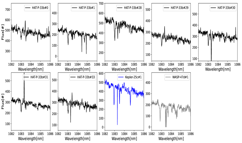
Figure 10: Exposures not considered in the analysis for the presence of outliers or low counts. Different colors correspond to different observing nights

.

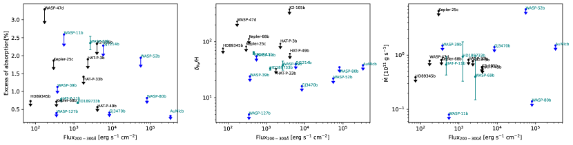
Figure 13: Correlation plots with the insolation level of mid-UV flux (200-300 Å). Same plot as in Fig. 8. As for the XUV flux between 5 and 504 Å, the He I absorption signal correlates with the received mid-UV flux; whereas when they are translated in terms of mass-loss rates, these trends seem to disappear.

Appendix B Gaussian processes to derive upper limits on the helium absorption

To have a better description of the correlated noise present in the data, we performed a Differential Evolution Markov chain Monte Carlo (DEMCMC) fit of a Gaussian profile fixing the position at 1083.326 nm and the FWHM at 0.07 nm and varying the peak value, an offset for the continuum, an uncorrelated jitter, and a correlated noise modeled with a Gaussian process (GP) and a squared exponential kernel. From the posterior distribution, we were therefore able to derive the 3$\sigma$ upper limits (the value to which 95% of the peak distribution is subject) at the position of the helium triplet marginalized over an uncorrelated jitter and the presence of correlated noise. The values are reported in Table 6.

Table 6: Upper limits on the excess of absorption.

Parameter	3$\sigma$[%]
HAT-P-3b	1.48
HAT-P-33b	1.17
HAT-P-49b	0.95
HD89345b	0.63
K2-105b	2.57
Kepler-25c	1.29
Kepler-68b	0.64
WASP-47d	3.11

References

- Akeson et al. (2013) Akeson, R. L., Chen, X., Ciardi, D., et al. 2013, PASP, 125, 989
- Allart et al. (2019) Allart, R., Bourrier, V., Lovis, C., et al. 2019, A&A, 623, A58
- Allart et al. (2018) Allart, R., Bourrier, V., Lovis, C., et al. 2018, Science, 362, 1384
- Allart et al. (2023) Allart, R., Lemée-Joliecoeur, P. B., Jaziri, A. Y., et al. 2023, arXiv e-prints, arXiv:2307.05580
- Allart et al. (2017) Allart, R., Lovis, C., Pino, L., et al. 2017, A&A, 606, A144
- Almenara et al. (2016) Almenara, J. M., Díaz, R. F., Bonfils, X., & Udry, S. 2016, A&A, 595, L5
- Alonso-Floriano et al. (2019) Alonso-Floriano, F. J., Snellen, I. A. G., Czesla, S., et al. 2019, A&A, 629, A110
- Attia et al. (2023) Attia, O., Bourrier, V., Delisle, J. B., & Eggenberger, P. 2023, A&A, 674, A120
- Attia et al. (2021) Attia, O., Bourrier, V., Eggenberger, P., et al. 2021, A&A, 647, A40
- Baluev et al. (2019) Baluev, R. V., Sokov, E. N., Jones, H. R. A., et al. 2019, MNRAS, 490, 1294
- Battley et al. (2021) Battley, M. P., Kunimoto, M., Armstrong, D. J., & Pollacco, D. 2021, MNRAS, 503, 4092
- Beaugé & Nesvorný (2013) Beaugé, C. & Nesvorný, D. 2013, ApJ, 763, 12
- Bennett et al. (2023) Bennett, K. A., Redfield, S., Oklopčić, A., et al. 2023, AJ, 165, 264
- Benomar et al. (2014) Benomar, O., Masuda, K., Shibahashi, H., & Suto, Y. 2014, PASJ, 66, 94
- Bieryla et al. (2014) Bieryla, A., Hartman, J. D., Bakos, G. Á., et al. 2014, AJ, 147, 84
- Bonomo et al. (2017) Bonomo, A. S., Desidera, S., Benatti, S., et al. 2017, A&A, 602, A107
- Bourrier et al. (2023) Bourrier, V., Attia, O., Mallonn, M., et al. 2023, A&A, 669, A63
- Bourrier et al. (2018) Bourrier, V., Lecavelier des Etangs, A., Ehrenreich, D., et al. 2018, A&A, 620, A147
- Brogi et al. (2018) Brogi, M., Giacobbe, P., Guilluy, G., et al. 2018, A&A, 615, A16
- Bryant & Bayliss (2022) Bryant, E. M. & Bayliss, D. 2022, AJ, 163, 197
- Cannon & Pickering (1993) Cannon, A. J. & Pickering, E. C. 1993, VizieR Online Data Catalog, III/135A
- Carleo et al. (2021) Carleo, I., Youngblood, A., Redfield, S., et al. 2021, AJ, 161, 136
- Casasayas-Barris et al. (2021a) Casasayas-Barris, N., Orell-Miquel, J., Stangret, M., et al. 2021a, A&A, 654, A163
- Casasayas-Barris et al. (2021b) Casasayas-Barris, N., Palle, E., Stangret, M., et al. 2021b, A&A, 647, A26
- Casasayas-Barris et al. (2020) Casasayas-Barris, N., Pallé, E., Yan, F., et al. 2020, A&A, 635, A206
- Castro-González et al. (2022) Castro-González, A., Díez Alonso, E., Menéndez Blanco, J., et al. 2022, MNRAS, 509, 1075
- Chan et al. (2011) Chan, T., Ingemyr, M., Winn, J. N., et al. 2011, AJ, 141, 179
- Claudi et al. (2017) Claudi, R., Benatti, S., Carleo, I., et al. 2017, European Physical Journal Plus, 132, 364
- Crossfield & Kreidberg (2017) Crossfield, I. J. M. & Kreidberg, L. 2017, AJ, 154, 6
- Cubillos et al. (2017) Cubillos, P., Harrington, J., Loredo, T. J., et al. 2017, AJ, 153, 3
- Cutri et al. (2003) Cutri, R. M., Skrutskie, M. F., van Dyk, S., et al. 2003, VizieR Online Data Catalog, II/246
- Czesla et al. (2022) Czesla, S., Lampón, M., Sanz-Forcada, J., et al. 2022, A&A, 657, A6
- Davis & Wheatley (2009) Davis, T. A. & Wheatley, P. J. 2009, MNRAS, 396, 1012
- Dethier & Bourrier (2023) Dethier, W. & Bourrier, V. 2023, A&A, 674, A86
- dos Santos et al. (2020a) dos Santos, L. A., Ehrenreich, D., Bourrier, V., et al. 2020a, A&A, 640, A29
- dos Santos et al. (2020b) dos Santos, L. A., Ehrenreich, D., Bourrier, V., et al. 2020b, A&A, 634, L4
- Dos Santos et al. (2022) Dos Santos, L. A., Vidotto, A. A., Vissapragada, S., et al. 2022, A&A, 659, A62
- Eastman et al. (2013) Eastman, J., Gaudi, B. S., & Agol, E. 2013, PASP, 125, 83
- Eggleton (1983) Eggleton, P. P. 1983, ApJ, 268, 368
- Ehrenreich et al. (2012) Ehrenreich, D., Bourrier, V., Bonfils, X., et al. 2012, A&A, 547, A18
- Ehrenreich et al. (2015) Ehrenreich, D., Bourrier, V., Wheatley, P. J., et al. 2015, Nature, 522, 459
- Fossati et al. (2022) Fossati, L., Guilluy, G., Shaikhislamov, I. F., et al. 2022, A&A, 658, A136
- Gaidos et al. (2022) Gaidos, E., Hirano, T., Beichman, C., et al. 2022, MNRAS, 509, 2969
- Gaidos et al. (2023) Gaidos, E., Hirano, T., Lee, R. A., et al. 2023, MNRAS, 518, 3777
- Gaidos et al. (2020a) Gaidos, E., Hirano, T., Mann, A. W., et al. 2020a, MNRAS, 495, 650
- Gaidos et al. (2020b) Gaidos, E., Hirano, T., Wilson, D. J., et al. 2020b, MNRAS, 498, L119
- Gajdoš et al. (2019) Gajdoš, P., Vaňko, M., & Parimucha, Š. 2019, Research in Astronomy and Astrophysics, 19, 041
- Giacobbe et al. (2021) Giacobbe, P., Brogi, M., Gandhi, S., et al. 2021, Nature, 592, 205
- Gilliland et al. (2013) Gilliland, R. L., Marcy, G. W., Rowe, J. F., et al. 2013, ApJ, 766, 40
- Grieves et al. (2018) Grieves, N., Ge, J., Thomas, N., et al. 2018, MNRAS, 481, 3244
- Guilluy et al. (2020) Guilluy, G., Andretta, V., Borsa, F., et al. 2020, A&A, 639, A49
- Guilluy et al. (2019) Guilluy, G., Sozzetti, A., Brogi, M., et al. 2019, A&A, 625, A107
- Gustafsson et al. (2008) Gustafsson, B., Edvardsson, B., Eriksson, K., et al. 2008, A&A, 486, 951
- Hartman et al. (2011) Hartman, J. D., Bakos, G. Á., Torres, G., et al. 2011, ApJ, 742, 59
- Hellier et al. (2012) Hellier, C., Anderson, D. R., Collier Cameron, A., et al. 2012, MNRAS, 426, 739
- Hirano et al. (2020) Hirano, T., Krishnamurthy, V., Gaidos, E., et al. 2020, ApJ, 899, L13
- Howe et al. (2014) Howe, A. R., Burrows, A., & Verne, W. 2014, ApJ, 787, 173
- Kanodia et al. (2020) Kanodia, S., Cañas, C. I., Stefansson, G., et al. 2020, ApJ, 899, 29
- Kanodia et al. (2022) Kanodia, S., Libby-Roberts, J., Cañas, C. I., et al. 2022, AJ, 164, 81
- Kasper et al. (2020) Kasper, D., Bean, J. L., Oklopčić, A., et al. 2020, AJ, 160, 258
- Kausch et al. (2015) Kausch, W., Noll, S., Smette, A., et al. 2015, A&A, 576, A78
- Kawauchi et al. (2022) Kawauchi, K., Murgas, F., Palle, E., et al. 2022, A&A, 666, A4
- Kirk et al. (2020) Kirk, J., Alam, M. K., López-Morales, M., & Zeng, L. 2020, AJ, 159, 115
- Kirk et al. (2022) Kirk, J., Dos Santos, L. A., López-Morales, M., et al. 2022, AJ, 164, 24
- Kreidberg (2015) Kreidberg, L. 2015, PASP, 127, 1161
- Kreidberg & Oklopčić (2018) Kreidberg, L. & Oklopčić, A. 2018, Research Notes of the American Astronomical Society, 2, 44
- Krishnamurthy et al. (2023) Krishnamurthy, V., Hirano, T., Gaidos, E., et al. 2023, MNRAS, 521, 1210
- Krishnamurthy et al. (2021) Krishnamurthy, V., Hirano, T., Stefánsson, G., et al. 2021, AJ, 162, 82
- Lammer et al. (2003) Lammer, H., Selsis, F., Ribas, I., et al. 2003, ApJ, 598, L121
- Lampón et al. (2020) Lampón, M., López-Puertas, M., Lara, L. M., et al. 2020, A&A, 636, A13
- Lavie et al. (2017) Lavie, B., Ehrenreich, D., Bourrier, V., et al. 2017, A&A, 605, L7
- Lecavelier Des Etangs (2007) Lecavelier Des Etangs, A. 2007, A&A, 461, 1185
- Lecavelier des Etangs et al. (2012) Lecavelier des Etangs, A., Bourrier, V., Wheatley, P. J., et al. 2012, A&A, 543, L4
- Lecavelier des Etangs et al. (2004) Lecavelier des Etangs, A., Vidal-Madjar, A., McConnell, J. C., & Hébrard, G. 2004, A&A, 418, L1
- Linsky et al. (2014) Linsky, J. L., Fontenla, J., & France, K. 2014, ApJ, 780, 61
- Livingston et al. (2018) Livingston, J. H., Crossfield, I. J. M., Petigura, E. A., et al. 2018, AJ, 156, 277
- Lopez & Fortney (2014) Lopez, E. D. & Fortney, J. J. 2014, ApJ, 792, 1
- Luo et al. (2018) Luo, A. L., Zhao, Y. H., Zhao, G., & et al. 2018, VizieR Online Data Catalog, V/153
- Mallonn et al. (2022) Mallonn, M., Poppenhaeger, K., Granzer, T., Weber, M., & Strassmeier, K. G. 2022, A&A, 657, A102
- Mancini et al. (2018) Mancini, L., Esposito, M., Covino, E., et al. 2018, A&A, 613, A41
- Mansfield et al. (2018) Mansfield, M., Bean, J. L., Oklopčić, A., et al. 2018, ApJ, 868, L34
- Marcy et al. (2014) Marcy, G. W., Isaacson, H., Howard, A. W., et al. 2014, The Astrophysical Journal Supplement Series, 210, 20
- Matsakos & Königl (2016) Matsakos, T. & Königl, A. 2016, ApJ, 820, L8
- Migaszewski & Goździewski (2018) Migaszewski, C. & Goździewski, K. 2018, MNRAS, 480, 1767
- Mills et al. (2019) Mills, S. M., Howard, A. W., Weiss, L. M., et al. 2019, AJ, 157, 145
- Mounzer et al. (2022) Mounzer, D., Lovis, C., Seidel, J. V., et al. 2022, A&A, 668, A1
- Murray-Clay et al. (2009) Murray-Clay, R. A., Chiang, E. I., & Murray, N. 2009, ApJ, 693, 23
- Narita et al. (2017) Narita, N., Hirano, T., Fukui, A., et al. 2017, PASJ, 69, 29
- Ninan et al. (2020) Ninan, J. P., Stefansson, G., Mahadevan, S., et al. 2020, ApJ, 894, 97
- Nortmann et al. (2018) Nortmann, L., Pallé, E., Salz, M., et al. 2018, Science, 362, 1388
- Oklopčić (2019) Oklopčić, A. 2019, ApJ, 881, 133
- Oklopčić & Hirata (2018) Oklopčić, A. & Hirata, C. M. 2018, ApJ, 855, L11
- Orell-Miquel et al. (2022) Orell-Miquel, J., Murgas, F., Pallé, E., et al. 2022, A&A, 659, A55
- Owen (2019) Owen, J. E. 2019, Annual Review of Earth and Planetary Sciences, 47, 67
- Owen & Lai (2018) Owen, J. E. & Lai, D. 2018, MNRAS, 479, 5012
- Owen et al. (2023) Owen, J. E., Murray-Clay, R. A., Schreyer, E., et al. 2023, MNRAS, 518, 4357
- Owen & Wu (2017) Owen, J. E. & Wu, Y. 2017, ApJ, 847, 29
- Palle et al. (2020) Palle, E., Nortmann, L., Casasayas-Barris, N., et al. 2020, A&A, 638, A61
- Paragas et al. (2021) Paragas, K., Vissapragada, S., Knutson, H. A., et al. 2021, ApJ, 909, L10
- Parker (1958) Parker, E. N. 1958, ApJ, 128, 664
- Plez (2012) Plez, B. 2012, Turbospectrum: Code for spectral synthesis
- Rainer et al. (2018) Rainer, M., Harutyunyan, A., Carleo, I., et al. 2018, in Society of Photo-Optical Instrumentation Engineers (SPIE) Conference Series, Vol. 10702, Ground-based and Airborne Instrumentation for Astronomy VII, 1070266
- Ryabchikova et al. (2015) Ryabchikova, T., Piskunov, N., Kurucz, R. L., et al. 2015, Physica Scripta, 90, 054005
- Salz et al. (2018) Salz, M., Czesla, S., Schneider, P. C., et al. 2018, A&A, 620, A97
- Salz et al. (2016) Salz, M., Czesla, S., Schneider, P. C., & Schmitt, J. H. M. M. 2016, A&A, 586, A75
- Sanchis-Ojeda et al. (2013) Sanchis-Ojeda, R., Winn, J. N., Marcy, G. W., et al. 2013, ApJ, 775, 54
- Sanz-Forcada et al. (2011) Sanz-Forcada, J., Micela, G., Ribas, I., et al. 2011, A&A, 532, A6
- Seager & Sasselov (2000) Seager, S. & Sasselov, D. D. 2000, ApJ, 537, 916
- Smette et al. (2015) Smette, A., Sana, H., Noll, S., et al. 2015, A&A, 576, A77
- Spake et al. (2018) Spake, J. J., Sing, D. K., Evans, T. M., et al. 2018, Nature, 557, 68
- Szabó & Kiss (2011) Szabó, G. M. & Kiss, L. L. 2011, ApJ, 727, L44
- Tripathi et al. (2015) Tripathi, A., Kratter, K. M., Murray-Clay, R. A., & Krumholz, M. R. 2015, ApJ, 808, 173
- Turner et al. (2017) Turner, J. D., Leiter, R. M., Biddle, L. I., et al. 2017, MNRAS, 472, 3871
- Van Eylen et al. (2018) Van Eylen, V., Dai, F., Mathur, S., et al. 2018, MNRAS, 478, 4866
- Vanderburg et al. (2017) Vanderburg, A., Becker, J. C., Buchhave, L. A., et al. 2017, AJ, 154, 237
- Vidal-Madjar et al. (2003) Vidal-Madjar, A., Lecavelier des Etangs, A., Désert, J. M., et al. 2003, Nature, 422, 143
- Vissapragada et al. (2022) Vissapragada, S., Knutson, H. A., Greklek-McKeon, M., et al. 2022, AJ, 164, 234
- Vissapragada et al. (2020) Vissapragada, S., Knutson, H. A., Jovanovic, N., et al. 2020, AJ, 159, 278
- Vissapragada et al. (2021) Vissapragada, S., Stefánsson, G., Greklek-McKeon, M., et al. 2021, AJ, 162, 222
- Wang et al. (2017) Wang, Y.-H., Wang, S., Liu, H.-G., et al. 2017, AJ, 154, 49
- Wyttenbach et al. (2020) Wyttenbach, A., Mollière, P., Ehrenreich, D., et al. 2020, A&A, 638, A87
- Yan et al. (2017) Yan, F., Pallé, E., Fosbury, R. A. E., Petr-Gotzens, M. G., & Henning, T. 2017, A&A, 603, A73
- Yu et al. (2018) Yu, L., Rodriguez, J. E., Eastman, J. D., et al. 2018, AJ, 156, 127
- Zeng & Sasselov (2014) Zeng, L. & Sasselov, D. 2014, ApJ, 784, 96
- Zhang et al. (2023) Zhang, M., Knutson, H. A., Dai, F., et al. 2023, AJ, 165, 62
- Zhang et al. (2022a) Zhang, M., Knutson, H. A., Wang, L., Dai, F., & Barragán, O. 2022a, AJ, 163, 67
- Zhang et al. (2022b) Zhang, M., Knutson, H. A., Wang, L., et al. 2022b, AJ, 163, 68
- Zhang et al. (2021) Zhang, M., Knutson, H. A., Wang, L., et al. 2021, AJ, 161, 181
Acknowledgements.
We thank the referee for the comments and suggestions. We thank V.l Andretta for his help. G.G. acknowledge financial contributions from PRIN INAF 2019, and from the agreement ASI-INAF number 2018-16-HH.0 (THE StellaR PAth project). R. A. is a Trottier Postdoctoral Fellow and acknowledges support from the Trottier Family Foundation. This work was supported in part by a grant from the Fonds de Recherche du Québec - Nature et Technologies (FRQNT). This work was funded by the Institut Trottier de Recherche sur les Exoplaneètes (iREx). This work has been carried out within the framework of the NCCR PlanetS supported by the Swiss National Sci- ence Foundation under grants 51NF40182901 and 51NF40205606. This project has received funding from the European Research Council (ERC) under the Eu- ropean Union’s Horizon 2020 research and innovation programme (project Spice Dune, grant agreement No 947634). This material reflects only the authors views and the Commission is not liable for any use that may be made of the information contained therein. This work has made use of the VALD database, operated at Uppsala University, the Institute of Astronomy RAS in Moscow, and the University of Vienna. This work has made use of the Turbospectrum code for spectral synthesisAppendix A Additional figures and tables