Combinatorics on Number Walls and the $p(t)$-adic Littlewood Conjecture

Abstract

Let $p$ be a prime number and $\alpha$ a real number. In analogy with the classical Littlewood Conjecture, de Mathan and Teulié conjectured that

$$\inf_{|m|\geq 1}|m|_{p}\cdot|m|\cdot|\left\langle\alpha m\right\rangle|=0$$

where $|m|$ is the usual absolute value, $|m|_{p}$ is the $p$-adic norm and $\left|\left\langle x\right\rangle\right|$ is the distance from $x\in\mathbb{R}$ to the nearest integer. This is the $p$-adic Littlewood Conjecture. Let $\mathbb{K}$ be a field and $p(t)$ be an irreducible polynomial with coefficients in $\mathbb{K}$. This paper deals with the analogue of this conjecture over the field of formal Laurent series over $\mathbb{K}$, known as the $p(t)$-adic Littlewood Conjecture ($p(t)$-LC).

Firstly, a given counterexample to $p(t)$-LC for the case $p(t)=t$ is shown to generate an explicit counterexample when $p(t)$ is any irreducible polynomial. Since Adiceam, Nesharim and Lunnon [1] proved the $p(t)$-LC is false when $p(t)=t$ and $\mathbb{K}$ has characteristic three, one obtains a disproof of the $p(t)$-LC over any such field in full generality (i.e for any choice of irreducible polynomial $p(t)$).

Secondly, a Khintchine-type theorem for $p(t)$-adic multiplicative approximation is established. This enables one to determine the measure of the set of counterexamples to $p(t)$-LC with an additional monotonic growth function. In complement to this result, the Hausdorff dimension of the same set is shown to be maximal when $p(t)=t$ in the critical case where the growth function is $\log^{2}$. These results here are in agreement with the corresponding theory of multiplicative Diophantine approximation over the reals.

These goals are achieved by developing an extensive theory in combinatorics relating $p(t)$-LC to the properties of the so-called number wall of a sequence. This is an infinite array containing the determinant of every finite Toeplitz matrix generated by that sequence. In full generality, the main novelty of this paper is creating a dictionary allowing one to transfer statements in Diophantine approximation in positive characteristic to combinatorics through the concept of a number wall, and conversely.

1 Introduction

Let $\alpha$ be a real number. Let $\left|\alpha\right|$ denote the usual absolute value and define $\left|\left\langle\alpha\right\rangle\right|$ as the distance from $\alpha$ to its nearest integer . A classical conjecture due to Littlewood states that for any real numbers $\alpha$ and $\beta$,

$$\inf_{n\in\mathbb{Z}\backslash\{0\}}\left|\left\langle n\alpha\right\rangle\right|\cdot\left|\left\langle n\alpha\right\rangle\right|\cdot\left|n\right|=0.$$

The Littlewood Conjecture (from now on abbreviated to LC) remains open. The current state of the art is a result by Einsiedler, Katok and Lindenstrauss [6], who proved the set of counterexamples to LC has Hausdorff dimension zero. In 2004, de Mathan and Teulié [15] suggested a variant commonly known as the $p$-adic Littlewood Conjecture (abbreviated to $p$-LC). Let $p$ be a prime number. Given a natural number $n$ expanded as $n=p^{k}\cdot n_{1}$, where $k$ and $n_{1}$ are natural numbers and $n_{1}$ and $p$ are coprime, define its $p$-adic norm as $|n|_{p}:=p^{-k}$.

Conjecture 1.0.1 ($\mathbf{p}$-LC, de Mathan and Teulié, 2004).

For any prime $p$ and any real number $\alpha$,

$$\inf_{n\in\mathbb{Z}\backslash\{0\}}|n|\cdot|n|_{p}\cdot|\langle n\alpha\rangle|=0.$$ (1.0.1)

In 2007, Einsiedler and Kleinbock [7] proved that the set of counterexamples to $p$-LC has Hausdorff dimension zero. Metric results have been obtained when a growth function is added to the left hand side of equation (1.0.1). Explicitly, for a non-decreasing function $f$ and prime number $p$, define the sets

$$W(f,p): =\left\{\alpha\in[0,1):\inf_{n\in\mathbb{N}\backslash\{0\}}f(n)\cdot n\cdot|n|_{p}\cdot\left|\left\langle\alpha\cdot n\right\rangle\right|=0\right\},$$ (1.0.2)

and

$$M(f,p)=[0,1)\backslash W(f,p).$$ (1.0.3)

That is, $W(f,p)$ is the set of real numbers in the unit interval satisfying $p$-LC with growth function $f$, and $M(f,p)$ is the set of those numbers failing it. In 2009, Bugeaud and Moshchevitin [4] proved that $M(\log^{2},p)$ has full Hausdorff dimension. Two years later, Bugeaud, Haynes and Velani [2] proved the Lebesgue measure of the same set is zero. Then, Badziahin and Velani [17] established that

$$\dim M(\log(n)\cdot\log(\log(n)),p)=1.$$

Above and throughout, $\dim$ refers to the Hausdorff dimension.

The $p$-adic Littlewood Conjecture admits a natural analogue over function fields. In order to state it, here and throughout this paper $q$ is a power of a prime number and $\mathbb{F}_{q}$ denotes the field with cardinality $q$. Additionally, $\mathbb{F}_{q}[t]$ is the ring of polynomials with coefficients in $\mathbb{F}_{q}$ and $(\mathbb{F}_{q}[t])_{n}$ is the subset of $\mathbb{F}_{q}[t]$ comprised of only the polynomials of degree less than or equal to $n\in\mathbb{N}$. Similarly, $\mathbb{F}_{q}(t)$ is the field of rational functions over $\mathbb{F}_{q}$. The absolute value of $\Theta(t)\in\mathbb{F}_{q}(t)$ is then

$$|\Theta(t)|=q^{\deg(\Theta(t))}.$$ (1.0.4)

The real and function field absolute values share a notation, and it will be clear from context which is meant. Using this metric, the completion of the field of rational functions is given by $\mathbb{F}_{q}((t^{-1}))$, the field of formal Laurent series in the variable $t^{-1}$ with coefficients in $\mathbb{F}_{q}$. An element $\Theta(t)$ of this field is written explicitly as

$$\Theta(t)=\sum^{\infty}_{i=-h}a_{i}t^{-i}$$ (1.0.5)

for some $h$ in $\mathbb{Z}$ and $a_{i}$ in $\mathbb{F}_{q}$ with $a_{h}\neq 0$. With this expression, the degree of $\Theta(t)\in\mathbb{F}_{q}((t^{-1}))$ is defined as $\deg(\Theta(t)):=h$. The fractional part of $\Theta(t)$ is given by

$$\langle\Theta(t)\rangle:=\sum^{\infty}_{i=1}a_{i}t^{-i}.$$

In analogy with the real numbers, the unit interval $\mathbb{I}$ is defined as

$$\mathbb{I}=\{\Theta(t)\in\mathbb{F}_{q}((t^{-1})):|\Theta(t)|<1\}.$$

Alternatively, it is the set containing exactly the fractional parts of every $\Theta(t)\in\mathbb{F}_{q}((t^{-1}))$.

The analogue of the prime numbers is the set of irreducible polynomials. Given such an irreducible polynomial $p(t)\in\mathbb{F}_{q}[t]$, the following is used to define the analogue of the $p$-adic norm: any $\Theta(t)\in\mathbb{F}_{q}((t^{-1}))$ can be expanded uniquely as

$$\Theta(t)=\sum^{\infty}_{i=-H}A_{i}(t)p(t)^{-i},$$

where $H=\left\lfloor\frac{\deg(\Theta(t))}{\deg(p(t))}\right\rfloor$ and $A_{i}(t)\in(\mathbb{F}_{q}[t])_{\deg(p(t))-1}$ for $i\geq-H$. This is known as the base $p(t)$ expansion of $\Theta(t)$ and it is unique and well-defined. Let $m$ be the degree of $p(t)$ and let $N(t)\in\mathbb{F}_{q}[t]$ be a polynomial with base $p(t)$ expansion $N(t):=\sum_{i=0}^{h}A_{i}(t)p(t)^{i}$. The $p(t)$-adic norm of $N(t)$ is defined as

$$|N(t)|_{p(t)}=q^{-mi},\text{ where }i=\min\{j\geq 0:A_{j}\neq 0\}.$$

The function field analogue of $p$-LC, also due to de Mathan and Teulié [15], reads as follows:

Conjecture 1.0.2 ($\mathbf{p(t)}$-adic Littlewood Conjecture, de Mathan and Teulié, 2004).

For any irreducible polynomial $p(t)$ in $\mathbb{F}_{q}[t]$ and any Laurent series $\Theta(t)\in\mathbb{F}_{q}((t^{-1}))$,

$$\inf_{N(t)\in\mathbb{F}_{q}[t]\backslash\{0\}}|N(t)|\cdot|N(t)|_{p(t)}\cdot\left|\left\langle N(t)\cdot\Theta(t)\right\rangle\right|=0.$$

The $p(t)$-adic Littlewood Conjecture is abbreviated to $p(t)$-LC. When $p(t)=t$, it becomes the $t$-adic Littlewood Conjecture (abbreviated to $t$-LC). In the same paper as it was conjectured, de Mathan and Teulié establish that $t$-LC is false over infinite fields. This work was extended by Bugeaud and de Mathan [3], who provide explicit counterexamples to $t$-LC in this case, whilst also providing examples of power series satisfying $t$-LC in any characteristic.

Over finite fields, $p(t)$-LC is more challenging. In 2017, Einsiedler, Lindenstrauss and Mohammadi [8] proved results on the positive characteristic analogue of the measure classification results of Einsiedler, Katok and Lindenstrauss [6], but their work falls short of implying that $p(t)$-LC fails on a set of Hausdorff dimension zero. In 2021, Adiceam, Nesharim and Lunnon [1] found an explicit counterexample to $t$-LC over $\mathbb{F}_{q}$, for $q$ a power of 3. They conjectured that the same Laurent series is a counterexample over $\mathbb{F}_{q}$ for $q$ a power of any prime congruent to 3 modulo 4. From this breakthrough, it is tempting to believe that $p(t)$-LC is false over all finite fields and for all irreducible polynomials $p(t)$. The first result in this paper provides further evidence to this claim by showing that any counterexample to $t$-LC induces a counterexample to $p(t)$-LC for any irreducible $p(t)$. This result thus reduces the problem of totally disproving $p(t)$-LC to only disproving $t$-LC. It is not expected that such a transference result should exist over $\mathbb{R}$.

Theorem 1.0.3 (Transference between $p(t)$-LC and $t$-LC).

Let $l$ be a natural number, $p(t)$ be an irreducible polynomial of degree $m$ over $\mathbb{F}_{q}$ and

$$\Theta(t):=\sum_{i=1}^{\infty}b_{i}t^{-i}\in\mathbb{F}_{q}((t^{-1}))$$ (1.0.6)

be a Laurent series. Assume that

$$\inf_{N(t)\in\mathbb{F}_{q}[t]\backslash\{0\}}|N(t)|\cdot|N(t)|_{t}\cdot\left|\left\langle N(t)\cdot\Theta(t)\right\rangle\right|=q^{-l}.$$ (1.0.7)

Then, the Laurent series $\Theta(p(t))\in\mathbb{F}_{q}((p(t)^{-1}))\subset\mathbb{F}_{q}((t^{-1}))$ satisfies

$$\inf_{N(t)\in\mathbb{F}_{q}[t]\backslash\{0\}}|N(t)|\cdot|N(t)|_{p(t)}\cdot\left|\left\langle N(t)\cdot\Theta(p(t))\right\rangle\right|=q^{-lm}.$$ (1.0.8)

In particular, if $\Theta(t)$ is a counterexample to $t$-LC in the sense that the infimum in equation (1.0.7) is positive, then $\Theta(p(t))$ is a counterexample to $p(t)$-LC in the sense that the infimum in equation (1.0.8) is positive.

Combining this with the counterexamples from Adiceam, Nesharim and Lunnon [1] and de Mathan and Bugeaud [3] leads to the following corollary:

Corollary 1.0.4.

For all irreducible polynomials $p(t)$, the $p(t)$-adic Littlewood Conjecture is false over infinite fields and also over any field of characteristic 3.

The remaining theorems in this paper are of a metric nature. The implicit measure used in the related statements is the Haar measure over $\mathbb{F}_{q}((t^{-1})))$, denoted by $\mu$. For an integer $l$, define a ball of radius $q^{-l}$ around a Laurent series $\Theta(t)\in\mathbb{F}_{q}((t^{-1}))$ as

$$B\left(\Theta(t),q^{-l}\right)=\left\{\Phi\in\mathbb{F}_{q}((t^{-1})):|\Theta(t)-\Phi(t)|\leq q^{-l}\right\}.$$ (1.0.9)

Explicitly, this set consists of all the Laurent series which have the same coefficients as $\Theta(t)$ up to and including the power of $t^{-l}$. The Haar measure over $\mathbb{F}_{q}((t^{-1}))$ is characterised by its translation invariance: for any $l\in\mathbb{N}$ and any $\Theta(t)\in\mathbb{F}_{q}((t^{-1}))$

$$\mu(B(\Theta(t),q^{-l}))=q^{-l}.$$

Let $f:\{0\}\cup\{q^{n}:n\in\mathbb{N}\}\to\mathbb{R}^{+}$ be a monotonic increasing function. The following sets are the natural analogues of those defined in (1.0.2) and (1.0.3):

$$W(f,p(t)): =\left\{\Theta\in\mathbb{I}:\inf_{N(t)\in\mathbb{F}_{q}[t]\backslash\{0\}}f(|N(t)|)\cdot|N(t)|\cdot|N(t)|_{p(t)}\left|\left\langle\Theta\cdot N(t)\right\rangle\right|=0\right\}$$ (1.0.10)

and

$$M(f,p(t)):=\left\{\Theta\in\mathbb{I}:\inf_{N(t)\in\mathbb{F}_{q}[t]\backslash\{0\}}f(|N(t)|)\cdot|N(t)|_{(p(t))}\cdot|N(t)|\cdot|\langle\Theta\cdot N(t)\rangle|>0\right\}.$$ (1.0.11)

Thus, $W(f,p(t))$ is the set of Laurent series satisfying $p(t)$-LC with growth function $f$, and $M(f,p(t))$ is the complement of $W(f,p(t))$.

Theorem 1.0.3 suggests $t$-LC underpins $p(t)$-LC, and hence the study of $t$-LC instead of the more general $p(t)$-LC is justified. The strategy for the remainder of this paper is to rephrase $t$-LC using the concept of a number wall. Section 3 provides a rigorous introduction to number walls, but for the sake of the introduction, the following definitions will suffice. A matrix is Toeplitz if every entry on a given diagonal is equal. It is thus determined by the sequence comprising its first column and row. The number wall of a sequence $S=(s_{i})_{i\in\mathbb{Z}}$ is a two dimensioanl array containing the determinants of all the possible finite Toeplitz matrices generated by consecutive elements of $S$. Specifically, the entry in row $m$ and column $n$ is the determinant of the $(m+1)\times(m+1)$ Toeplitz matrix with top left entry $s_{n}$. Zero entries in number walls can only appear in square shapes, called windows. The key insight of this paper is the following theorem, which reduces the Diophantine problem underpinning $t$-LC to combinatorics on number walls:

Theorem 1.0.5.

Let $\Theta(t)=\sum_{i=1}^{\infty}s_{i}t^{-i}\in\mathbb{F}_{q}((t^{-1}))$, $l$ be a natural number and $f:\mathbb{N}\to\mathbb{R}$ be a positive monotonic increasing function. The following are equivalent:

1. The inequality

   $$\inf_{N(t)\in\mathbb{F}_{q}[t]\backslash\{0\}}f(|N(t)|)\cdot|N(t)|\cdot|N(t)|_{t}\cdot|\langle N(t)\cdot\Theta(t)\rangle|\geq q^{-l}.$$

   is satisfied (In particular, $\Theta(t)$ is a counterexample to the $t$-LC with growth function $f$).

2. For every $m,n\in\mathbb{N}$, there is no window of size greater than or equal to $l+\lceil\log_{q}(f(q^{m+n}))\rceil-1$ with top left corner on row $m$ and column $m+n+1$ in the number wall generated by the sequence $S=(s_{i})_{i\in\mathbb{N}}$.

Above, $\log_{q}(x)$ is the base-$q$ logarithm of a real number $x$. Sections 3 develops an extensive theory of combinatorics on number walls, resulting in explicit formulae for how many finite sequences have a given window in their number wall. Section 5 extends these results to count how many finite sequences have any given pair of disconnected windows, or a window containing any given connected zero portion. These combinatorial results are hence used to prove a Khintchine-type result on $p(t)$-adic multiplicative approximation.

Theorem 1.0.6.

Let $f:\{0\}\cup\{q^{k}\}_{k\geq 0}\to\mathbb{R}+$ be a monotonic increasing function and $p(t)\in\mathbb{F}_{q}[t]$ be an irreducible polynomial. Then

$$\mu(W(f,p(t)))=\begin{cases}0&\text{ if }\sum_{k\geq 0}\frac{k}{f(q^{k})}<\infty\\ 1&\text{ if }\sum_{k\geq 0}\frac{k}{f(q^{k})}=\infty\end{cases}.$$ (1.0.12)

This amounts to claiming that the set of counterexamples to $p(t)$-LC with growth function $f$ has zero or full measure depending on if the sum in (1.0.12) converges or diverges. This agrees with the analogous theorem over the real numbers, proved in [2] by Bugeaud, Haynes and Velani. The combinatorial theory developed to study the properties of number walls in Section 3 is also used to prove the final theorem in this paper, which computes the Hausdorff dimension of $M(f,p(t))$ in the case $p(t)=t$ and $f(|N|)=\log_{q}(|N|)^{2}$. Recalling Definition 1.0.3, this provides the function field analogue of the 2009 result by Bugeaud and Moshchevitin [4], stating $\dim M(\log^{2},p)=1$ in the real case.

Theorem 1.0.7.

The set of counterexamples to the $t$-LC with growth function $\log^{2}$ has full Hausdorff dimension. That is,

$$\dim(M(\log^{2},t))=1.$$

Note, that Theorem 1.0.7 is nontrivial as Theorem 1.0.6 implies that $M(\log^{2},t)$ has measure zero.

Acknowledgements

The Author is grateful to his supervisor Faustin Adiceam for his consistent support, supervision and advice throughout the duration of this project. Furthermore, the Author acknowledges the financial support of the Heilbronn Institute.

2 From Counterexamples to $t$-LC to Counterexamples to $p(t)$-LC

This chapter is dedicated to proving Theorem 1.0.3; namely that a counterexample to $t$-LC implies a counterexample to $p(t)$-LC for any irreducible $p(t)$. Decomposing the polynomial $N(t)$ as $p(t)\cdot N^{\prime}(t)$ for $N^{\prime}(t)\in\mathbb{F}_{q}[t]$ coprime to $p(t)$, the equation in (1.0.2) is rephrased as

$$\inf_{\begin{subarray}{c}N^{\prime}(t)\in\mathbb{F}_{q}[t]\backslash\{0\}\\ k\geq 0\end{subarray}}\left|\left\langle\Theta(t)\cdot N^{\prime}(t)\cdot p(t)^{k}\right\rangle\right|\cdot|N^{\prime}(t)|=0.$$ (2.0.1)

Due to the infimum being over all polynomials $N^{\prime}(t)$ and natural numbers $k$, it is simple to see that $N^{\prime}(t)$ being coprime to $p(t)$ is not required. Given a Laurent series $F(t)\in\mathbb{F}_{q}((x^{-1}))$, define $\deg_{x}(F(t))$ as the degree of $F(t)$ measured with respect to the variable $t$, and let $|F|^{(t)}:=q^{\deg_{t}(F)}$ be its norm. Throughout this section, $p(t)\in\mathbb{F}_{q}[t]$ is an irreducible polynomial and $m:=\deg_{t}(p(t))$.

Lemma 2.0.1.

Let $l$ be a natural number and $\Theta(t):=\sum_{i=0}^{\infty}s_{i}t^{-i}$ be a Laurent series in $\mathbb{F}_{q}((t^{-1}))$. Then,

$$\inf_{\begin{subarray}{c}N(t)\in\mathbb{F}_{q}[t]\backslash\{0\}\\ k\geq 0\end{subarray}}\left|\left\langle\Theta(t)\cdot N(t)\cdot t^{k}\right\rangle\right|^{(t)}\cdot|N(t)|^{(t)}=q^{-l}$$ (2.0.2)

if and only if

$$\inf_{\begin{subarray}{c}N(p(t))\in\mathbb{F}_{q}[p(t)]\backslash\{0\}\\ k\geq 0\end{subarray}}\left|\left\langle\Theta(p(t))\cdot N(p(t))\cdot p(t)^{k}\right\rangle\right|^{(t)}\cdot|N(p(t))|^{(t)}=q^{-ml}.$$ (2.0.3)

Proof of Lemma 2.0.1.

Let $N(t)=\sum^{h}_{j=0}a_{j}t^{j}$ be a nonzero polynomial in $\mathbb{F}_{q}[t]$. Define $h:=\deg_{t}N(t)$. Then, (2.0.3) holds if and only if

$$\left|\left\langle\Theta(p(t))\cdot N(p(t))\cdot p(t)^{k}\right\rangle\right|^{(t)}\geq q^{-m(l+h)}$$ (2.0.4)

for any positive integer $k$. Furthermore,

$$\left\langle\Theta(p(t))\cdot N(p(t))\cdot p(t)^{k}\right\rangle =\left\langle\left(\sum^{\infty}_{i=1}s_{i}p(t)^{-i}\right)\cdot\left(\sum^{h}_{j=0}a_{j}p(t)^{j}\right)\cdot p(t)^{k}\right\rangle$$

$$=\left\langle\sum^{\infty}_{i=1}\left(\sum^{h}_{j=0}a_{j}s_{i+j+k}\right)p(t)^{-i}\right\rangle,$$

implying that

$$\deg_{t}\left(\left\langle\Theta(p(t))\cdot N(p(t))\cdot p(t)^{k}\right\rangle\right)\in\left\{-mn:n\geq 1\right\},$$ (2.0.5)

as the expansion of $p(t)^{-i}$ has degree $-im$, since $p(t)^{i}\cdot p(t)^{-i}=1$. Relation (2.0.5) and the definition of the absolute value (1.0.4) imply that (2.0.4) holds if and only if, for any positive integer $k$, there exists some $1\leq i\leq l+h$ such that $\sum^{h}_{j=0}a_{j}s_{i+j+k}\neq 0$. Explicitly, this means that the system of equations

$$\begin{pmatrix}s_{1+k}&s_{2+k}&\dots&s_{h+1+k}\\ s_{2+k}&s_{3+k}&\dots&s_{h+2+k}\\ \vdots&&&\vdots\\ s_{l^{\prime}+h+k}&s_{l^{\prime}+h+k+1}&\dots&s_{l^{\prime}+2h+k}\\ \end{pmatrix}\begin{pmatrix}a_{0}\\ a_{1}\\ \vdots\\ a_{h}\end{pmatrix}=\begin{pmatrix}0\\ \vdots\\ 0\\ \end{pmatrix}$$

has no non trivial solution. This condition is independent of the choice of $p(t)$, and holds in particular when $p(t)=t$. This shows the equivalency of (2.0.2) and (2.0.3). ∎

Completion of the proof of Theorem 1.0.3..

Consider a polynomial $N(t)\in\mathbb{F}_{q}[t]\backslash\{0\}$ expanded in base $p(t)$ as:

$$N(t)=\sum_{i=0}^{h^{\prime}}A_{i}(t)p(t)^{i}$$

with $h^{\prime}:=\left\lfloor\frac{\deg_{t}{N(t)}}{m}\right\rfloor$ and $\deg_{t}(A_{i}(t))\leq m-1$ for every $0\leq i\leq h^{\prime}$. Let $a_{j,i}$ be the coefficient of $t^{j}$ in $A_{i}(t)$. Then,

$$N(t)=\sum_{i=0}^{h^{\prime}}\sum^{m-1}_{j=0}a_{j,i}t^{j}p(t)^{i}=\sum^{m-1}_{j=0}t^{j}\sum_{i=0}^{h^{\prime}}a_{j,i}p(t)^{i}:=\sum^{m-1}_{j=0}t^{j}N_{j}(p(t)),$$ (2.0.6)

where $N_{j}(p(t)):=\sum^{h^{\prime}}_{i=0}a_{j,i}p(t)^{i}\in\mathbb{F}_{q}[p(t)]$. Therefore,

$$\inf_{\begin{subarray}{c}N(t)\in\mathbb{F}_{q}[t]\backslash\{0\}\\ k\geq 0\end{subarray}} \left|\left\langle\Theta(p(t))\cdot N(t)\cdot p(t)^{k}\right\rangle\right|^{(t)}\cdot|N(t)|^{(t)}$$

$$=\inf\leavevmode\nobreak\ \left|\left\langle\Theta(p(t))\cdot\sum^{m-1}_{j=0}t^{j}N_{j}(p(t))\cdot p(t)^{k}\right\rangle\right|^{(t)}\cdot\left|\sum^{m-1}_{j=0}t^{j}N_{j}(p(t))\right|^{(t)}$$

$$=\inf\leavevmode\nobreak\ \left|\sum^{m-1}_{j=0}\left\langle\Theta(p(t))\cdot t^{j}N_{j}(p(t))\cdot p(t)^{k}\right\rangle\right|^{(t)}\cdot\left|\sum^{m-1}_{j=0}t^{j}N_{j}(p(t))\right|^{(t)}.$$ (2.0.7)

Above, and throughout the rest of the proof, the infimum is taken over natural numbers $k\geq 0$ and all polynomials $N_{0}(p(t)),\dots,N_{m-1}(p(t))\in\mathbb{F}_{q}[p(t)]$, ignoring the case where they are all zero. It is clear that $\left\langle\Theta(p(t))\cdot N(p(t))\cdot p(t)^{k}\right\rangle$ has no nonzero coefficient for $t^{-1},\dots,t^{-m+1}$, which implies that for any $0\leq j\leq m-1$,

$$\left\langle\Theta(p(t))\cdot t^{j}N(p(t))\cdot p(t)^{k}\right\rangle=t^{j}\left\langle\Theta(p(t))\cdot N(p(t))\cdot p(t)^{k}\right\rangle.$$

Hence,

$$(\ref{inf1})=\inf\leavevmode\nobreak\ \left|\sum^{m-1}_{j=0}t^{j}\left\langle\Theta(p(t))\cdot N_{j}(p(t))\cdot p(t)^{k}\right\rangle\right|^{(t)}\cdot\left|\sum^{m-1}_{j=0}t^{j}N_{j}(p(t))\right|^{(t)}\cdotp$$ (2.0.8)

If the degree of $\left\langle\Theta(p(t))\cdot N(p(t))\cdot p(t)^{k}\right\rangle$ is $-nm$, then for any $0\leq j\leq m-1$ the degree of $t^{j}\left\langle\Theta(p(t))\cdot N(p(t))\cdot p(t)^{k}\right\rangle$ is $-nm+j\equiv j\mod m$. This implies that the degree of each of the terms in $\sum^{m-1}_{j=0}t^{j}\left\langle\Theta(p(t))\cdot N_{j}(p(t))\cdot p(t)^{k}\right\rangle$ are all different and therefore the degree of the sum is equal to the greatest degree of its terms. The same is true for $\left|\sum^{m-1}_{j=0}t^{j}N_{j}(p(t))\right|^{(t)}$. As a consequence,

$$(\ref{inf3}) =\inf\leavevmode\nobreak\ \max_{j\in\{0,\dots,m-1\}}\left|t^{j}\left\langle\Theta(p(t))\cdot N_{j}(p(t))\cdot p(t)^{k}\right\rangle\right|^{(t)}\max_{i\in\{0,\dots,m-1\}}\left|t^{i}N_{i}(p(t))\right|^{(t)}$$

$$=\inf\leavevmode\nobreak\ \max_{j\in\{0,\dots,m-1\}}q^{j}\left|\left\langle\Theta(p(t))\cdot N_{j}(p(t))\cdot p(t)^{k}\right\rangle\right|^{(t)}\max_{i\in\{0,\dots,m-1\}}q^{i}\left|N_{i}(p(t))\right|^{(t)}.$$ (2.0.9)

Let $j^{\prime}$ and $i^{\prime}$ be the values of $j$ and $i$, respectively, that attain the maxima in (2.0.9). Then,

$$\max_{j\in\{0,\dots,m-1\}}q^{j}\left|\left\langle\Theta(p(t))\cdot N_{j}(p(t))\cdot p(t)^{k}\right\rangle\right|^{(t)}\leavevmode\nobreak\ \max_{i\in\{0,\dots,m-1\}}q^{i}\left|N_{i}(p(t))\right|^{(t)}$$

$$\geq\min_{\leavevmode\nobreak\ h\in\{j^{\prime},i^{\prime}\}}q^{h}\left|\left\langle\Theta(p(t))\cdot N_{h}(p(t))\cdot p(t)^{k}\right\rangle\right|^{(t)}q^{h}\left|N_{h}(p(t))\right|^{(t)}$$

$$\underset{(\ref{inf5})}{\geq}q^{-ml+2h}$$

This provides a lower bound for the value of (2.0.9), namely the case where $h=0$. The fact that $\mathbb{F}_{q}[p(t)]\subset\mathbb{F}_{q}[t]$ and the equation (2.0.3) show that this lower bound is attained, hence

$$(\ref{inf4})=q^{-lm}.$$

This completes the proof of Theorem 1.0.3. ∎

The next section proves the link between $t$-LC and number walls and develops the combinatorial theory required to prove Theorem 1.0.7.

3 Combinatorial Properties of Number Walls

3.1 Fundamentals of Number Walls

This section serves as an introduction to number walls. Only the theorems crucial for this paper are mentioned, and the proofs can be found in the references. For a more comprehensive look at number walls, see [1, Section 3],[5, pp 85-89], [13] and [14]. The following definition provides the building blocks of a number wall.

Definition 3.1.1.

A matrix $(s_{i,j})$ for $0\leq i\leq n,0\leq j\leq m$ is called Toeplitz (Hankel, respectively) if all the entries on a diagonal (on an anti-diagonal, respectively) are equal. Equivalently, $s_{i,j}=s_{i+1,j+1}$ ($s_{i,j}=s_{i+1,j-1}$, respectively) for any $n\in\mathbb{N}$ such that this entry is defined.

Given a doubly infinite sequence $S:=(s_{i})_{i\in\mathbb{Z}}$, natural numbers $m$ and $v$, and an integer $n$, define an $(m+1)\times(v+1)$ Toeplitz matrix $T_{S}(n,m,v):=(s_{i-j+n})_{0\leq i\leq m,0\leq j\leq v}$ and a Hankel matrix of the same size as $H_{A}(n,m,v):=(s_{i+j+n})_{0\leq i\leq m,0\leq j\leq v}$:

$$T_{S}(n,m,v):=\begin{pmatrix}s_{n}&s_{n+1}&\dots&s_{n+v}\\ s_{n-1}&s_{n}&\dots&s_{n+v-1}\\ \vdots&&&\vdots\\ s_{n-m}&s_{n-m+1}&\dots&s_{n-m+v}\end{pmatrix}, H_{S}(n,m,v):=\begin{pmatrix}s_{n}&s_{n+1}&\dots&s_{n+v}\\ s_{n+1}&s_{n+2}&\dots&s_{n+v+1}\\ \vdots&&&\vdots\\ s_{n+m}&s_{n+m+1}&\dots&s_{n+m+v}\end{pmatrix}.$$

If $v=m$, these are shortened to $T_{S}(n,m)$ and $H_{S}(n,m)$, respectively. The Laurent series $\Theta(t)=\sum^{\infty}_{i=1}s_{i}t^{-1}\in\mathbb{F}_{q}((t^{-1}))$ is identified to the sequence $S=(s_{i})_{i\geq 1}$. Therefore, define $T_{\Theta}(n,m,v)=T_{S}(n,m,v)$ and $H_{\Theta}(n,m,v):=H_{S}(n,m,v)$.

By elementary row operations, it holds that.

$$\det(H_{A}(n,m))=(-1)^{\frac{m(m+1)}{2}}\det(T_{A}(n+m,m)).$$ (3.1.1)

Definition 3.1.2.

Let $S=(s_{i})_{i\in\mathbb{Z}}$ be a doubly infinite sequence over a finite field $\mathbb{F}_{q}$. The number wall of the sequence $S$ is defined as the two dimensional array of numbers $W(S)=(W_{m,n}(S))_{n,m\in\mathbb{Z}}$ with

$$W_{m,n}(S)=\begin{cases}\det(T_{S}(n,m))&\textup{ if }m\geq 0\\ 1&\textup{ if }m=-1\\ 0&\textup{ if }m<-1,\end{cases}$$

In keeping with standard matrix notation, $m$ increases as the rows go down the page and $n$ increases from left to right.

A key feature of number walls is that the zero entries can only appear in specific shapes:

Theorem 3.1.3 (Square Window Theorem).

Zero entries in a Number Wall can only occur within windows; that is, within square regions with horizontal and vertical edges.

Proof.

See [14, page 9]. ∎

For the problems under consideration, the zero windows carry the most important information in the number wall. Theorem 3.1.3 implies that the border of a window is always the boundary of a square with nonzero entries. This motivates the following definition:

Definition 3.1.4.

The entries of a number wall surrounding a window are referred to as the inner frame. The entries surrounding the inner frame form the outer frame.

The entries of the inner frame are extremely well structured:

Theorem 3.1.5.

The inner frame of a window with side length $l\geq 1$ is comprised of 4 geometric sequences. These are along the top, left, right and bottom edges and they have ratios $P,Q,R$ and $S$ respectively with origins at the top left and bottom right. Furthermore, these ratios satisfy the relation

$$\frac{PS}{QR}=(-1)^{l}.$$

Proof.

See [14, Page 11]. ∎

See Figure 1 for an example of a window of side length $l$. For $i\in\{0,\dots,l+1\}$, the inner and outer frames are labelled by the entries $A_{i},B_{i},C_{i},D_{i}$ and $E_{i},F_{i},G_{i},H_{i}$ respectively. The ratios of the geometric sequences comprising the inner frame are labelled as $P,Q,R$ and $S$.

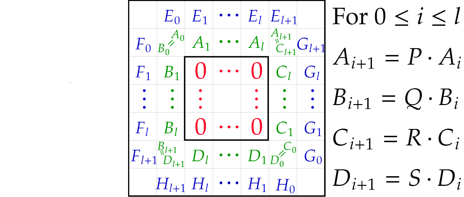
Figure 1: Illustration of a window in a number wall. The window, inner frame and outer frame are in red, green and blue, respectively.

Calculating a number wall from its definition is a computationally exhausting task. The following theorem gives a simple and far more efficient way to calculate the $m^{\textup{th}}$ row using the previous rows.

Theorem 3.1.6 (Frame Constraints).

Given a doubly infinite sequence $S=(s_{i})_{i\in\mathbb{Z}}$, the number wall $(W_{m,n})_{n,m\in\mathbb{Z}}:=(W_{m,n}(S))_{n,m\in\mathbb{Z}}$ can be generated by a recurrence in row $m\in\mathbb{Z}$ in terms of the previous rows. More precisely, with the notation of Figure 1,

$$W_{m,n}=\begin{cases}\begin{aligned} &0&&\textup{ if }m<-1\textup{ or if }(m,n)\textup{ is within a window;}&\\ &1&&\textup{ if }m=-1;&\\ &s_{n}&&\textup{ if }m=0;&\\ &\frac{W_{m-1,n}^{2}-W_{m-1,n-1}W_{m-1n+1}}{W_{m-2,n}}&&\textup{ if }m>0\textup{ and }W_{m-2,n}\neq 0;&\\ &D_{k}=\frac{(-1)^{l\cdot k}B_{k}C_{k}}{A_{k}}&&\textup{ if }m>0\textup{ and }W_{m-2,n}=0=W_{m-1,n};&\\ &H_{k}=\frac{\frac{QE_{k}}{A_{k}}+(-1)^{k}\frac{PF_{k}}{B_{k}}-(-1)^{k}\frac{SG_{k}}{C_{k}}}{R/D}&&\textup{ if }m>0\textup{ and }W_{n,m-2}=0\neq W_{n,m-1}.&\end{aligned}\end{cases}$$

Proof.

See [14, Page 11] ∎

The value of $k$ above is found in the natural way from the value of $m,n$ and the side length $l$. The final three equations above are known as the First, Second and Third Frame Constraint equations. These allow the number wall of a sequence to be considered independently of its original definition in terms of Toeplitz matrices.

Theorem 1.0.5 provides the link between $t$-LC and number walls. The following lemma is required for the proof.

Lemma 3.1.7.

Let $H=(s_{i+j-1})$ with $1\leq i,j\leq n$ be an $m\times m$ Hankel matrix with entries in $\mathbb{F}_{q}$. Assume that the first $r$ columns of $H$ are linearly independent but that the first $r+1$ columns are linearly dependent (here, $1\leq r\leq m-1$). Then the principal minor of order r, that is, $\det(s_{i+j-1})_{1\leq i,j\leq r}$, does not vanish.

Proof.

See [1, Lemma 2.3] or [18, Chapter 10]. ∎

Proof of Theorem 1.0.5..

$1\Rightarrow 2:$ The proof is by contraposition. Let $N(t)=M(t)\cdot t^{n}\in\mathbb{F}_{q}[t]$ be a nonzero polynomial with $M(t)$ coprime to $t$. Let $m$ be the degree of $M(t):=\sum_{i=0}^{m}a_{i}t^{i}$. From the definition of the $t$-adic norm,

$$f(|N(t)|)\cdot|N(t)|\cdot|N(t)|_{t}\cdot|\langle\Theta(t)\cdot N(t)\rangle| =f(q^{m+n})\cdot q^{m}\cdot|\langle\Theta(t)\cdot M(t)\cdot t^{n}\rangle|.$$ (3.1.2)

This quantity is strictly less than $q^{-l}$ if and only if

$$|\langle\Theta(t)\cdot M(t)\cdot t^{n}\rangle|<q^{-l-m-b_{f}^{(q)}(m+n)},$$ (3.1.3)

where $b_{f}^{(q)}(m+n)=\lceil\log_{q}(f(q^{m+n}))\rceil$. This is equivalent to the coefficients of $t^{-i}$ in $\langle\Theta(t)\cdot M(t)\cdot t^{n}\rangle$ being zero for $i\in\{1,\dots,l+m+b_{f}^{(q)}(m+n)\}.$ This coefficient is given by

$$\sum_{j=0}^{m}a_{j}s_{i+j+n},$$

and hence the inequality (3.1.3) can be written as the matrix equation

$$H_{\Theta}(1+n,l+m+b_{f}^{(q)}(m+n)-1,m)\cdot\begin{pmatrix}a_{0}\\ \vdots\\ a_{m}\end{pmatrix}=\mathbf{0}.$$ (3.1.4)

This implies that $H_{\Theta}(n+1,l+m+b_{f}^{(q)}(m+n)-1,m)$ has less than maximal rank, meaning the square matrix $H_{\Theta}(n+1,l+m+b_{f}^{(q)}(m+n)-1)$ has zero determinant. In particular, $H_{\Theta}(n+1,i)$ is singular for $m\leq i\leq l+m+b_{f}^{(q)}(m+n)-1$, since each of these matrices satisfies the same linear recurrence relation in the first $m+1$ columns.

Relation (3.1.1) shows that the determinant of $H_{\Theta}(n+1,i)$ is, up to a nonzero multiplicative constant, equal to the determinant of $T_{\Theta}(n+1+i,i)$. Therefore, there is a diagonal of zeros from entry $(n+m+1,m)$ to entry $(n+m+l+b_{f}^{(q)}(m+n),m+l+b_{f}^{(q)}(m+n)-1).$ The Square Window Theorem (Theorem 3.1.3) implies that there is a window of size $l+b_{f}^{(q)}(m+n)$ in row $m$ and column $m+n+1$.

$2\Rightarrow 1:$ Proceeding again by contraposition, assume that there is a window of size $l+b_{f}^{(q)}(m+n)$ in row $m$ and column $n+m+1$ for some $m,n\in\mathbb{N}$. The diagonal of this window corresponds to a sequence of nested singular square Toeplitz matrices, $T_{\Theta}(n+1+i,i)$ for $m\leq i\leq l+m+b_{f}^{(q)}(m+n)-1$. Hence, the matrices $H_{\Theta}(n+1,i)$ for $i$ in the same range are all singular. The largest of these Hankel matrices in this diagonal is singular and thus it has linearly dependent columns. Since the second largest is also singular, Lemma 3.1.7 implies that the first $m+l+b_{f}^{(q)}(m+n)-1$ columns are linearly dependent. Furthermore, since the third largest matrix is also singular this implies that the first $m+l+b_{f}^{(q)}(m+n)-2$ columns are linearly dependent. A simple induction shows that $H_{\Theta}(n+1,l+m+b_{f}^{(q)}(m+n)-1,m)$ has less than maximal rank.

Let then $\mathbf{a}=(a_{0},\dots,a_{m})^{\top}\in\mathbb{F}_{q}^{m+1}$ be a vector such that $H_{\Theta}(n+1,l+m+b_{f}^{(q)}(m+n)-1,m)\cdot\mathbf{a}=\mathbf{0}$. Define the polynomials $M(t)=\sum_{i=0}^{m}a_{i}t^{i}$ and $N(t):=M(t)\cdot t^{n}$. By the same steps used to obtain (3.1.3) and (3.1.4), one has that

$$f(|N(t)|)\cdot|N(t)|\cdot|N(t)|_{t}\cdot|\langle\Theta(t)\cdot N(t)\cdot t^{n}\rangle|<q^{-l}.$$

Hence, a polynomial $N=M\cdot t^{n}$ with $m:=\deg(M)$ and $(M,t)=1$ being a solution to

$$f(|N|)\cdot|N|\cdot|N|_{t}\cdot\left\langle N\cdot\Theta\right\rangle<q^{-l}$$

is equivalent to there being a window of size $l+b_{f}^{(q)}(m+n)$ on row $m$ and column $m+n+1$. This completes the proof.
∎

Taking $f$ to be the constant function, the following corollary becomes clear.

Corollary 3.1.8.

Let $\Theta(t)=\sum^{\infty}_{i=1}s_{i}t^{-i}\in\mathbb{F}_{q}((t^{-1}))$ be a Laurent series and $S=(s_{i})_{i\in\mathbb{N}}$ be the sequence of its coefficients. Then, $\Theta(t)$ is a counterexample to $t$-LC if and only if there exists an $l$ in the natural numbers such that the number wall of $(s_{i})_{i\geq 0}$ has no windows of size larger than $l$.

A finite number wall is a number wall generated by a finite sequence. The next subsection begins to develop the combinatorial theory on finite number walls.

3.2 The Free-Determined Lemma

The proofs of Theorems 1.0.6 and 1.0.7 involve extending a finite number wall to satisfy the growth condition from Theorem 1.0.5 in the size of its windows. To this end, the following definitions and lemmas illustrate basic properties of a finite number wall.

Definition 3.2.1.

For a finite sequence $S$ and its number wall $W(S)$, the depth of $W(S)$ is defined as the greatest value of the row index $m$ such that the entry $W_{m,n}(S)$ is defined for some column index $n\in\mathbb{Z}$.

It is simple to see that a finite sequence of length $r$ generates a number wall in the shape of an isosceles triangle with depth $\left\lfloor\frac{r-1}{2}\right\rfloor$. To make number walls visually accessible, each entry is given a unique colour depending on its value (See Figure 3). Every number wall shown in this paper is coloured with the same colour scheme. Whilst generating number walls can be insightful, it provides no help if one is trying to prove a result for number walls in general. The introduction of dot diagrams remedies this by giving a way to visualise an arbitrary number wall of finite size, allowing for a clearer exposition during proofs. A blank dot diagram can be seen below.

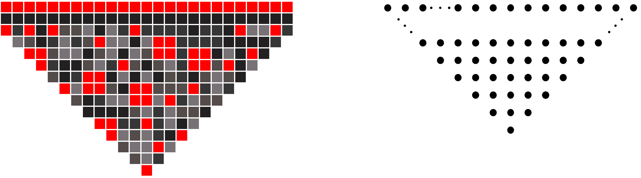
Figure 2: Left: The number wall of a sequence of length 25 generated uniformly and randomly over $\mathbb{F}_{5}$. The zero entries are coloured in red, with the nonzero values assigned a shade of grey, with 1 being the darkest and 4 being the lightest. The top row (red) hasindex $-2$. Right: A blank dot diagram.

Each dot in the dot diagram represents an entry of the number wall, with the top row representing the sequence generating the number wall. The dot diagram in Figure 3 contains no information, but as the paper progresses dot diagrams are used to convey information about the structure and construction of a number wall. Numbers above an entry on the top row of a dot diagram indicate how many choices there are in $\mathbb{F}_{q}$ for that entry resulting in the indicated diagram. This is first seen in Figure 13.

The next lemma in this subsection shows that number walls behave well under symmetry.

Lemma 3.2.2.

Let $W(S)$ be the number wall of the finite sequence $S=(s_{1},\dots,s_{r})$. Define $S^{\prime}=(s_{r},\dots,s_{1})$ as the ‘reflection’ of $S$. Then the number wall of $S^{\prime}$ is the number wall of $S$, reflected vertically. More precisely, let $m$ and $n$ be natural numbers satisfying $0\leq m\leq\left\lfloor\frac{r-1}{2}\right\rfloor$ and $0\leq n\leq r-1-2m$, and define $W_{m,n}(S)$ and $W_{m,n}(S^{\prime})$ to be the entry on column $n$ and row $m$ of the number walls of $S$ and $S^{\prime}$, respectively. Then $W_{r-m-n,m}(S^{\prime})=W_{m+n+1,m}(S)$.

Proof.

The entry of $W(S)$ in column $m+n+1$ and row $m$ is equal to the determinant of $T_{S}(m+n+1,m)$. Similarly, the entry in column $r-m-n$ and row $m$ of $W(S^{\prime})$ is $T_{S^{\prime}}(r-m-n,m)$. The definition of $T_{S^{\prime}}(r-m-n,m)$ shows it is the transpose of $T_{S}(m+n+1,m)$, completing the proof. ∎

Lemma 3.2.2 is illustrated by Figure 3:

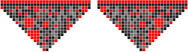
Figure 3: Left: The number wall of a sequence $S$ over $\mathbb{F}_{5}$. Each entry of $S$ is picked with equal probability assigned to every value of $\mathbb{F}_{5}$. Right: The number wall of $S^{\prime}$, defined as in Lemma 3.2.2.

The following definitions are introduced to facilitate the extension of a finite number wall.

Definition 3.2.3.

Let $S=(s_{i})_{1\leq i\leq r}$ be a finite sequence of length $r$, and let $W(S)=(W_{m,n}(S))_{m,n\in\mathbb{Z}}$ be the number wall generated by $S$. Assume that $s_{r+1}$ is to be added to the end of the sequence $S$. Then:

• The $\mathbf{k^{\text{th}}}$ diagonal is all the elements of the number wall with column index $k-i$ and row index $i$ for $0\leq i\leq\left\lfloor\frac{k-1}{2}\right\rfloor$.

• An entry on the $(r+1)^{\textup{th}}$ diagonal of the number wall generated by $S\cup\{s_{r+1}\}$ is determined if it is independent of the choice of $s_{r+1}$.

• An entry $W_{i,r+1-i}(S\cup\{s_{r+1}\})$ of the number wall on the $(r+1)^{\textup{th}}$ diagonal is free if for any $x\in\mathbb{F}_{q}$, there exists a value of $s_{r+1}$ in the first row making $W_{i,r+1-i}(S)=x$.

Given a finite number wall generated by a sequence of length $r$, the following lemma describes how many degrees of freedom there are for the values of the $(r+1)^{\textup{th}}$ diagonal.

Lemma 3.2.4 (Free-Determined Lemma).

Let $W(S)=(W_{m,n}(S))_{n,m\in\mathbb{Z}}$ be the finite number wall generated by the sequence $S=(s_{i})_{0\leq i\leq r}$. Assume that $s_{r+1}$ is added to the end of $S$. Then, for $0\leq i\leq\left\lfloor\frac{r}{2}\right\rfloor$, $W_{i,r+1-i}(S)$ is determined if and only if $W_{i-1,r-i}(S)=0$. Furthermore, if $W_{i,r+1-i}(S)$ is not determined, then it is free. In particular, picking a value for any non-determined entry on the $(r+1)^{\textup{th}}$ diagonal uniquely decides the value for every remaining non-determined entry on the $(r+1)^{\textup{th}}$ diagonal.

Proof.

The value of $W_{i,r+1-i}(S)$ is calculated from the definition of a number wall:

$$W_{i,r+1-i}(S)=\det(T_{S}(r+1-i,i))=\det\begin{pmatrix}s_{r+1-i}&\dots&s_{r+1}\\ \vdots&\ddots&\vdots\\ s_{r+1-2i}&\dots&s_{r+1-i}\end{pmatrix}.$$

Due to the Toeplitz structure, $s_{r+1}$ only occurs in the top right corner of $T_{S}(r+1-i,i)$. By expanding along the top row,

$$W_{i,r+1-i}(S)=s_{r+1}\cdot\det(T_{S}(r-i,i-1))+Y,$$

where $Y$ is a number that depends only on $\{s_{i}:1\leq i\leq r\}$. Hence, the value of $W_{i,r+1-i}(S)$ is independent of $s_{r+1}$ if and only if $\det(T_{S}(r-i,i-1))=W_{i-1,r-i}(S)=0$. If $W_{i-1,r-i}(S)\neq 0$, then for any chosen value of $W_{i,r+1-i}(S)$ there exists a unique choice of $s_{r+1}$ that achieves it. Namely,

$$s_{r+1}=(W_{i,r+1-i}(S)-Y)\cdot\det(T_{S}(r-i,i-1))^{-1}.$$ (3.2.1)

This, in turn, fixes the value of every non-determined entry on diagonal $r+1.$ ∎

The Free-Determined Lemma (Lemma 3.2.4) has the following simple corollary:

Corollary 3.2.5.

Let $S=(s_{i})_{0\leq i\leq r}$ be a finite sequence. Define the sequences $S^{\prime}$ and $S^{\prime\prime}$ as the sequence $S$ with an additional element, $s_{r+1}^{\prime}$ and $s_{r+1}^{\prime\prime}$, respectively, added on the end. If $0\leq j\leq\left\lfloor\frac{r}{2}\right\rfloor$ is such that $W_{j,r+1-j}(S^{\prime})$ and $W_{j,r+1-j}(S^{\prime\prime})$ are not determined, then $W_{j,r+1-j}(S^{\prime})=W_{j,r+1-j}(S^{\prime\prime})$ if and only if $s_{r+1}^{\prime}=s_{r+1}^{\prime\prime}$.

Proof.

Clearly, if $s_{r+1}^{\prime}=s_{r+1}^{\prime\prime}$, then the entire $(r+1)^{\textup{th}}$ diagonal is identical. Hence, assume that $W_{j,r+1-j}(S^{\prime})=W_{j,r+1-j}(S^{\prime\prime})$. By Corollary 3.2.4, this also fixes the value for every non-determined entry in the diagonal. Furthermore, by definition the values on the top row cannot be determined, which completes the proof. ∎

Remark 3.2.6.

That $t$-LC (and hence $p(t)$-LC from Theorem 1.0.3) are false over infinite fields $\mathbb{K}$ (originally established by Mathan and Teulié in [15]) is an immediate consequence of Lemma 3.2.4. Indeed, if the sequence $(s_{i})_{1\leq i\leq r}$ over $\mathbb{K}$ has no windows in its number wall, every entry on the $(r+1)^{\textup{th}}$ diagonal is free. Now, Lemma 3.2.4 shows there are infinite choices for $s_{1+r}$ that do not create any windows. A simple induction beginning with any nonzero sequence of length one generates a counterexample to $t$-LC.

Lemma 3.2.4 explains when a finite sequence can be extended by one digit to obtain a particular value in the number wall. In practice, finite sequences are not extended one digit at a time, but instead by arbitrarily many digits at once. The next subsection proves results about how many ways this can be done whilst preserving certain properties of the number wall.

3.3 The Blade of a Finite Number Wall

Understanding the bottom two rows of a finite number wall is at the heart of the proofs of Theorems 1.0.6 and 1.0.7. This motivates the following definition:

Definition 3.3.1.

Given a finite number wall, define its blade as the values on the bottom two rows. Explicitly, if the number wall is generated by a sequence of length $r\in\mathbb{N}$, then the blade is rows $\left\lfloor\frac{r-1}{2}\right\rfloor$ and $\left\lfloor\frac{r-1}{2}\right\rfloor-1$. Furthermore, define the right-side (left-side, respectively) blade as entries in the two right-most (left-most, respectively) columns of the blade.

These definitions are illustrated below:

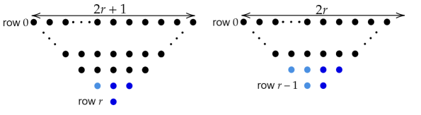
Figure 4: The blades of these number walls are coloured in blue, with the right-side blade in a darker shade. If the finite sequence has odd length the right-side blade and the left-side blade overlap.

Studying the right-side blade is sufficient for most purposes, but all of the results in this sub-section are also true for the left-side blade by symmetry from Lemma 3.2.2. It is often only important that an entry in the number wall is zero or nonzero, with its exact value in the latter case being irrelevant, whence this definition:

Definition 3.3.2.

Let $W(S)$ be the number wall of a sequence $S$. The shape of $W(S)$ is a two dimensional array with the same width and height as $W(S)$ where every non-zero entry has been replaced with the same symbol. In other words, the shape of a number wall shows only where its zero entries are located.

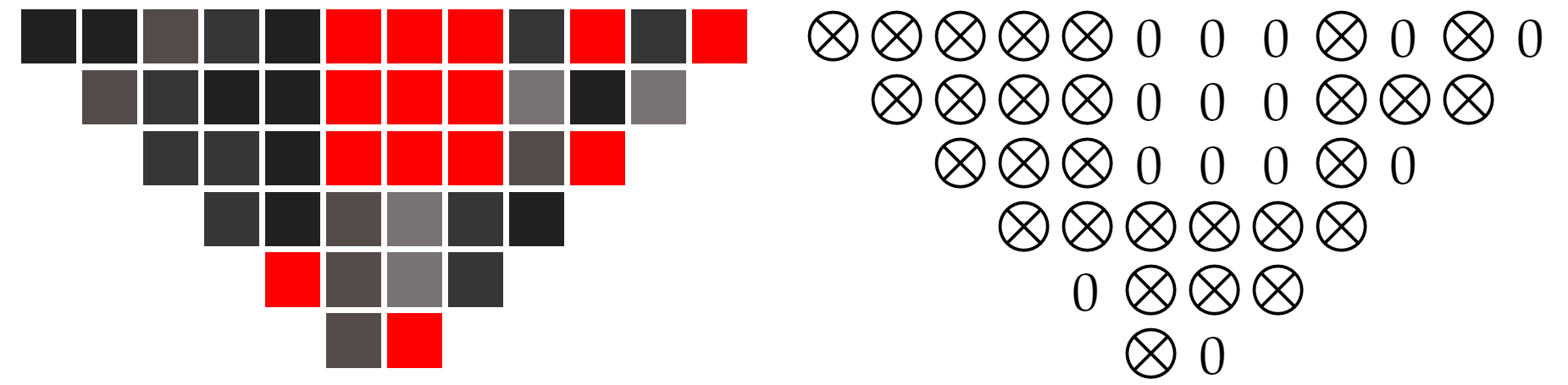
Figure 5: Left: The number wall $W(S)$ for the sequence $S=(1,1,3,2,1,0,0,0,2,0,2,0)\in\mathbb{F}_{5}^{12}$. The windows are coloured in red. Right: The shape of $W(S)$.

This definition allows for dot diagrams to distinguish between zero and nonzero entries without worrying about specific values. Using this notation, there are seven possible shapes for the right-side blade, as the shape with a nonzero entry in the top left and zeros in the top right and bottom left is not possible due to the Square Window Theorem (Theorem 3.1.3).

Figure 6: The seven possible right-side blade shapes.

In text, these right-side blade shapes are denoted by $\begin{subarray}{c}\phantom{X}XX\\ X\end{subarray},\leavevmode\nobreak\ \begin{subarray}{c}\phantom{I}X0\\ X\end{subarray},\leavevmode\nobreak\ \begin{subarray}{c}\phantom{X}0X\\ X\end{subarray},\leavevmode\nobreak\ \begin{subarray}{c}\phantom{X}XX\\ 0\end{subarray},\leavevmode\nobreak\ \begin{subarray}{c}\phantom{X}0\phantom{i}0\\ X\end{subarray},\leavevmode\nobreak\ \begin{subarray}{c}\phantom{X}0X\\ 0\end{subarray},\leavevmode\nobreak\ \begin{subarray}{c}\phantom{0}\hskip 1.0pt0\hskip 1.0pt0\\ 0\end{subarray}.$ The right-side blade comprised of all zeros (furthest right in Figure 6) is called the zero right-side blade. All other blades are described as nonzero.

Let $S=(s_{i})_{1\leq i\leq r}$ be a finite sequence of length $r$ in $\mathbb{F}_{q}$ whose number wall has a nonzero right-side blade. There are $q^{2}$ different ways to add $s_{r+1}$ and $s_{r+2}$ to the end of $S$, forming a sequence $S^{\prime}$ of length $r+2$. These $q^{2}$ continuations can be partitioned by the different blades they create in the number wall of $S^{\prime}$. Indeed, let $\{u_{i}\}_{i=1,2,3}$ and $\{v_{i}\}_{i=1,2,3}$ be the entries in the right-side blade of the sequence $S$ and $S^{\prime}$ respectively.

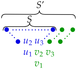
Figure 7: How $u_{1},u_{2},u_{3},v_{1},v_{2}$ and $v_{3}$ appear in the number wall of $S^{\prime}$.

Using Lemma 3.2.4, the following diagrams are created. Each shows a given right-side blade shape for $S$ (in blue, representing $u_{1},u_{2}$ and $u_{3}$) and all the possible right-side blade shapes for $S^{\prime}$ (in green, representing $v_{1},v_{2}$ and $v_{3}$), with the number of possible continuations from $S$ to $S^{\prime}$ giving this right-side blade written underneath. These are referred to as the Tree Diagrams. There are six in total, and two of them are explained in detail. The rest follows similarly.

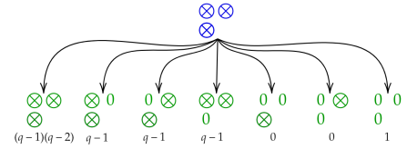
Figure 8: The $\begin{subarray}{c}\phantom{X}XX\\ X\end{subarray}$-Tree Diagram.

In this case, using the notation from Figure 7, all the values of $\{u_{i}\}_{i=1,2,3}$ are nonzero, and hence Lemma 3.2.4 implies all the values $\{v_{i}\}_{i=1,2,3}$ are free. Lemma 3.2.4 also implies there is only one choice of $s_{r+1}$ that would give $v_{2}=0$, and hence there are $q-1$ choices that give $v_{2}\neq 0$. In the same way, there are unique choices of $s_{r+2}$ that give $v_{1}=0$ and $v_{3}=0$. These choices coincide if and only if $v_{2}=0$, explaining the final green right-side blade in Figure 8. Furthermore, if $v_{2}\neq 0$ then it is impossible that $v_{1}=0=v_{3}$ by the Square Window Theorem (Theorem 3.1.3). Hence, there are $(q-2)$ choices for $s_{r+2}$ making neither $v_{1}$ or $v_{3}$ zero, giving $(q-1)(q-2)$ choices for $s_{r+1}$ and $s_{r+2}$ resulting in the first green right-side blade in Figure 8. The same reasoning explains the second and fourth right-side blades. Because the sequence $S$ has right-side blade $\begin{subarray}{c}\phantom{X}XX\\ X\end{subarray}$, it is impossible for $S^{\prime}$ to have right-side blade $\begin{subarray}{c}\phantom{X}0X\\ 0\end{subarray}$ or $\begin{subarray}{c}\phantom{X}0\phantom{i}0\\ X\end{subarray}$, as this would result in a non-square window. Therefore, there are $q-1$ ways to obtain the third right-side blade.

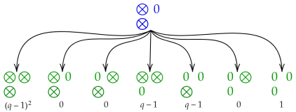
Figure 9: The $\begin{subarray}{c}\phantom{I}X0\\ X\end{subarray}$-Tree Diagram.

This is much the same as the $\begin{subarray}{c}\phantom{X}XX\\ X\end{subarray}$-Tree Diagram, but now the value of $v_{3}$ are determined. However, it still depends on the value of $s_{r+1}$, and $v_{2}$ is free. Hence, there is one choice for $s_{r+1}$ making $v_{2}=0$ and $q-1$ choices for $s_{r+1}$ giving $v_{2}\neq 0$. In the latter case, it is impossible to have $v_{3}=0$ as this would create two windows touching diagonally, violating the Square Window Theorem (Theorem 3.1.3). This explains the second right-side blade. However, $v_{1}$ is free and hence there are $q-1$ choices for $s_{r+1}$ making it nonzero and a single choice making it zero, explaining the first and fifth right-side blade. The third and sixth right-side blades are impossible due to the Square Window Theorem (Theorem 3.1.3). The third and seventh right-side blades follow exactly as in Figure 8.

The remaining Tree Diagrams are shown below. The reader is encouraged to verify them to gain a better understanding.

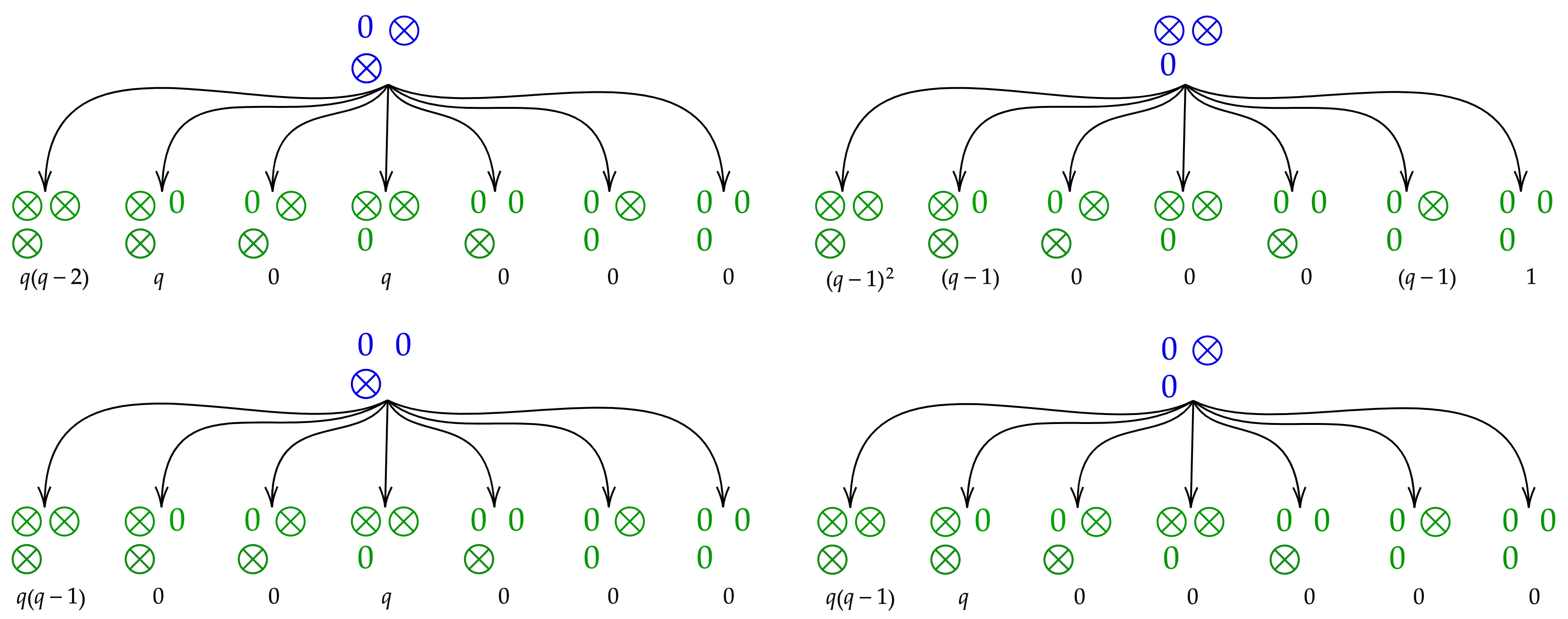
Figure 10: Top left: The $\begin{subarray}{c}\phantom{X}0X\\ X\end{subarray}$-Tree Diagram. Top right: The $\begin{subarray}{c}\phantom{X}XX\\ 0\end{subarray}$-Tree Diagram. Bottom left: The $\begin{subarray}{c}\phantom{X}0\phantom{i}0\\ X\end{subarray}$-Tree Diagram. Bottom right: The $\begin{subarray}{c}\phantom{X}0X\\ 0\end{subarray}$-Tree Diagram.

Note that there is no $\begin{subarray}{c}\phantom{0}\hskip 1.0pt0\hskip 1.0pt0\\ 0\end{subarray}$-Tree Diagram. This is because the values of $\{v_{i}\}_{i=1,2,3}$ are all determined and depend on the values of $\{s_{i}\}_{1\leq i\leq r-2}$.

Given a finite sequence $S$ with a nonzero right-side blade, the Tree Diagrams show how many length-two continuations of $S$ give any desired right-side blade. The function introduced in the following definition generalises this to continuations of any arbitrary even length.

Definition 3.3.3.

Let $B_{1},B_{2}$ denote the nonzero right-side blade shapes $\begin{subarray}{c}\phantom{X}XX\\ X\end{subarray},\begin{subarray}{c}\phantom{I}X0\\ X\end{subarray}$, or $\begin{subarray}{c}\phantom{X}XX\\ 0\end{subarray}$. Define the function

$$Q :\{\begin{subarray}{c}\phantom{X}XX\\ X\end{subarray},\begin{subarray}{c}\phantom{I}X0\\ X\end{subarray},\begin{subarray}{c}\phantom{X}XX\\ 0\end{subarray}\}^{2}\times\mathbb{N}\to\mathbb{N},$$

$$(B_{1},B_{2},m)\mapsto Q(B_{1},B_{2},m)$$

as the number of ways a finite sequence whose number wall has right-side blade $B_{1}$ can be extended by $2m$ entries such that the number wall of the resulting sequence has right-side blade $B_{2}$.

For example, $Q(\begin{subarray}{c}\phantom{X}XX\\ X\end{subarray},\begin{subarray}{c}\phantom{X}0\phantom{i}0\\ X\end{subarray},1)$ is the number of ways a finite sequence whose number wall has right-side blade $\begin{subarray}{c}\phantom{X}XX\\ X\end{subarray}$ can be extended by two digits to have a right-side blade $\begin{subarray}{c}\phantom{X}0\phantom{i}0\\ X\end{subarray}$. The $\begin{subarray}{c}\phantom{X}XX\\ X\end{subarray}$-Tree Diagram shows that $Q(\begin{subarray}{c}\phantom{X}XX\\ X\end{subarray},\begin{subarray}{c}\phantom{X}0\phantom{i}0\\ X\end{subarray},1)=0$.

Although it is not clear a priori, the map $Q$ is well defined. This is justified below, in Lemma 3.3.4. The same lemma gives explicit values of $Q(B_{1},B_{2},m)$. These formulas do not need to be committed to memory and are not individually important. They are used later in the proof of Lemma 3.4.4.

Lemma 3.3.4.

Let $B_{1}$ and $B_{2}$ be nonzero right-side blades and $m$ be a natural number. Then the function $Q(B_{1},B_{2},m)$ is well-defined. Explicitly, the value of $Q(B_{1},B_{2},m)$ only depends on the stated variables, and not any other values in the number wall. Furthermore, $Q(B_{1},B_{2},m)$ takes the following values for $m\geq 1$:

1. 1. $Q(\begin{subarray}{c}\phantom{X}0\phantom{i}0\\ X\end{subarray},\begin{subarray}{c}\phantom{X}XX\\ X\end{subarray},m)=Q(\begin{subarray}{c}\phantom{X}0X\\ 0\end{subarray},\begin{subarray}{c}\phantom{X}XX\\ X\end{subarray},m)=\begin{cases}\frac{q(q-1)^{2}}{q+1}(q^{2m-2}-1)&\text{ if }m\geq 2\\ q(q-1)&\text{ if }m=1.\end{cases}$.

   2. $Q(\begin{subarray}{c}\phantom{X}0X\\ X\end{subarray},\begin{subarray}{c}\phantom{X}XX\\ X\end{subarray},m)=\begin{cases}\frac{q(q-1)}{q+1}(q^{2m-1}-q^{2m-2}+2)&\text{ if }m\geq 2\\ q(q-2)&\text{ if }m=1.\end{cases}$

   3. $Q(\begin{subarray}{c}\phantom{X}XX\\ X\end{subarray},\begin{subarray}{c}\phantom{X}XX\\ X\end{subarray},m)=\frac{q-1}{q+1}(q^{2m}-q^{2m-1}-2)$.

   4. $Q(\begin{subarray}{c}\phantom{I}X0\\ X\end{subarray},\begin{subarray}{c}\phantom{X}XX\\ X\end{subarray},m)=Q(\begin{subarray}{c}\phantom{X}XX\\ 0\end{subarray},\begin{subarray}{c}\phantom{X}XX\\ X\end{subarray},m)=\frac{(q-1)^{2}}{q+1}(q^{2m-1}+1)$.

2. 1. $Q(\begin{subarray}{c}\phantom{X}XX\\ X\end{subarray},\begin{subarray}{c}\phantom{I}X0\\ X\end{subarray},m)=Q(\begin{subarray}{c}\phantom{X}XX\\ 0\end{subarray},\begin{subarray}{c}\phantom{I}X0\\ X\end{subarray},m)=\frac{q-1}{q+1}(q^{2m-1}+1)$

   2. $Q(\begin{subarray}{c}\phantom{I}X0\\ X\end{subarray},\begin{subarray}{c}\phantom{I}X0\\ X\end{subarray},m)=\begin{cases}\frac{q(q-1)}{q+1}(q^{2m-2}-1)&\text{ if }m\geq 2\\ 0&\text{ if }m=1\end{cases}$

   3. $Q(\begin{subarray}{c}\phantom{X}0X\\ X\end{subarray},\begin{subarray}{c}\phantom{I}X0\\ X\end{subarray},m)=Q(\begin{subarray}{c}\phantom{X}0X\\ 0\end{subarray},\begin{subarray}{c}\phantom{I}X0\\ X\end{subarray},m)=\begin{cases}\frac{q(q-1)}{q+1}(q^{2m-2}-1)&\text{ if }m\geq 2\\ q&\text{ if }m=1\end{cases}$

   4. $Q(\begin{subarray}{c}\phantom{X}0\phantom{i}0\\ X\end{subarray},\begin{subarray}{c}\phantom{I}X0\\ X\end{subarray},m)=\begin{cases}\frac{q^{2}(q-1)}{q+1}(q^{2m-3}+1)&\text{ if }m\geq 2\\ 0&\text{ if }m=1.\end{cases}$

3. 1. $Q(\begin{subarray}{c}\phantom{X}XX\\ X\end{subarray},\begin{subarray}{c}\phantom{X}XX\\ 0\end{subarray},m)=Q(\begin{subarray}{c}\phantom{I}X0\\ X\end{subarray},\begin{subarray}{c}\phantom{X}XX\\ 0\end{subarray},m)=\frac{q-1}{q+1}(q^{2m-1}+1)$

   2. $Q(\begin{subarray}{c}\phantom{X}0X\\ X\end{subarray},\begin{subarray}{c}\phantom{X}XX\\ 0\end{subarray},m)=Q(\begin{subarray}{c}\phantom{X}0\phantom{i}0\\ X\end{subarray},\begin{subarray}{c}\phantom{X}XX\\ 0\end{subarray},m)=\begin{cases}\frac{q(q-1)}{q+1}(q^{2m-2}-1)&\text{ if }m\geq 2\\ q&\text{ if }m=1.\end{cases}$

   3. $Q(\begin{subarray}{c}\phantom{X}XX\\ 0\end{subarray},\begin{subarray}{c}\phantom{X}XX\\ 0\end{subarray},m)=\begin{cases}\frac{q(q-1)}{q+1}(q^{2m-2}-1)&\text{ if }m\geq 2\\ 0&\text{ if }m=1.\end{cases}$

   4. $Q(\begin{subarray}{c}\phantom{X}0X\\ 0\end{subarray},\begin{subarray}{c}\phantom{X}XX\\ 0\end{subarray},m)=\begin{cases}\frac{q^{2}(q-1)}{q+1}(q^{2m-3}+1)&\text{ if }m\geq 2\\ 0&\text{ if }m=0.\end{cases}$

Proof.

For the sake of brevity, the formulae are proved in triples: the value of $Q(B_{1},B_{2},m)$ is derived for a generic choice of $B_{2}$. To obtain an individual formula, a specification of the shape of $B_{2}$ is made and a simple calculation is performed. Each formulae will be referred to with the labels from Lemma 3.3.4.

The lemma is proved by induction on $m$. The base cases are given by the Tree Diagrams (Figures 8, 9 and 10), and it is clear these are well-defined. Assume that these formulas hold and that the function is well-defined up to $m-1$. The following dot diagram displays the situation:

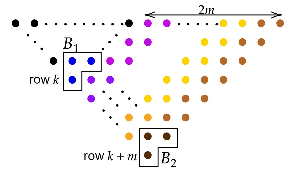
Figure 11: The black dots represent the starting number wall, with its right-side blade in blue. Each pair of colours represents an additional two entries being added to the sequence, with the right-side blade created by these additions being in a darker shade. This dot diagram assumes the starting sequence has odd length. In the even length case, the first element of the starting sequence can be entirely ignored, reducing back to the odd case.

Every formula is proved using the same idea. The Tree diagram for $B_{1}$ shows which possible shapes the right-side blade could take when the generating sequence is extended by two, and how many ways each shape occurs. For example, the $\begin{subarray}{c}\phantom{X}0\phantom{i}0\\ X\end{subarray}$-Tree Diagram (Figure 10) shows that when extending the sequence by two, there are $q(q-1)$ ($q$, respectively) ways to get a right-side blade of shape $\begin{subarray}{c}\phantom{X}XX\\ X\end{subarray}$ (of shape $\begin{subarray}{c}\phantom{X}XX\\ 0\end{subarray}$, respectively). With the notations of Definition 3.3.3, it is clear that

$$Q(\begin{subarray}{c}\phantom{X}0\phantom{i}0\\ X\end{subarray},B_{2},m)=q(q-1)\cdot Q(\begin{subarray}{c}\phantom{X}XX\\ X\end{subarray},B_{2},m-1)+q\cdot Q(\begin{subarray}{c}\phantom{X}XX\\ 0\end{subarray},B_{2},m-1).$$

Picking a specific right-side blade shape for $B_{2}$, using the induction hypothesis and doing some simple rearranging gives formulae $(1.1)$, $(2.4)$ and $(3.2)$. It is also clear from this recurrence formulae that, if $Q(\begin{subarray}{c}\phantom{X}XX\\ X\end{subarray},B_{2},m-1)$ and $Q(\begin{subarray}{c}\phantom{X}XX\\ 0\end{subarray},B_{2},m-1)$ are well-defined, then so is $Q(\begin{subarray}{c}\phantom{X}0\phantom{i}0\\ X\end{subarray},B_{2},m)$. Similarly, the $\begin{subarray}{c}\phantom{X}0X\\ 0\end{subarray}$- Tree Diagram (Figure 10) shows that

$$Q(\begin{subarray}{c}\phantom{X}0X\\ 0\end{subarray},B_{2},m)=q(q-1)\cdot Q(\begin{subarray}{c}\phantom{X}XX\\ X\end{subarray},B_{2},m-1)+q\cdot Q(\begin{subarray}{c}\phantom{I}X0\\ X\end{subarray},B_{2},m-1)$$

and the $\begin{subarray}{c}\phantom{X}0X\\ X\end{subarray}$-Tree Diagram (Figure 10) that

$$Q(\begin{subarray}{c}\phantom{X}0X\\ X\end{subarray},B_{2},m)=q(q-2)\cdot Q(\begin{subarray}{c}\phantom{X}XX\\ X\end{subarray},B_{2},m-1)+q\cdot Q(\begin{subarray}{c}\phantom{I}X0\\ X\end{subarray},B_{2},m-1)+q\cdot Q(\begin{subarray}{c}\phantom{X}XX\\ 0\end{subarray},B_{2},m-1).$$

Once again, picking a specific shape for $B_{2}$, using the induction hypothesis and rearranging proves the two equalities in $(1.1)$, $(2.3)$, and also the equalities $(3.4)$, $(1.2)$, and $(3.2)$.

The formulae for $B_{1}=\begin{subarray}{c}\phantom{X}XX\\ X\end{subarray},\leavevmode\nobreak\ \begin{subarray}{c}\phantom{I}X0\\ X\end{subarray}$ and $\begin{subarray}{c}\phantom{X}XX\\ 0\end{subarray}$ are not as simple. The formula for $Q(\begin{subarray}{c}\phantom{X}XX\\ X\end{subarray},B_{2},m)$ is first proved. Using the $\begin{subarray}{c}\phantom{X}XX\\ X\end{subarray}$-Tree Diagram (Figure 8),

$$Q(\begin{subarray}{c}\phantom{X}XX\\ X\end{subarray},B_{2},m)= (q-1)(q-2)\cdot Q(\begin{subarray}{c}\phantom{X}XX\\ X\end{subarray},B_{2},m-1)+(q-1)\cdot Q(\begin{subarray}{c}\phantom{I}X0\\ X\end{subarray},B_{2},m-1)$$

$$+(q-1)\cdot Q(\begin{subarray}{c}\phantom{X}0X\\ X\end{subarray},B_{2},m-1)+(q-1)\cdot Q(\begin{subarray}{c}\phantom{X}XX\\ 0\end{subarray},B_{2},m-1)$$

$$+\tilde{Q}_{\begin{subarray}{c}\phantom{X}XX\\ X\end{subarray}}(\begin{subarray}{c}\phantom{0}\hskip 1.0pt0\hskip 1.0pt0\\ 0\end{subarray},B_{2},m-1),$$ (3.3.1)

where $\tilde{Q}_{\begin{subarray}{c}\phantom{X}XX\\ X\end{subarray}}(\begin{subarray}{c}\phantom{0}\hskip 1.0pt0\hskip 1.0pt0\\ 0\end{subarray},B_{2},m-1)$ is the number of ways to add $2m$ digits to a generating sequence with right-side blade $\begin{subarray}{c}\phantom{X}XX\\ X\end{subarray}$, with the additional constraint that the first two digits result in the zero right-side blade. This is illustrated below:

Figure 12: $\tilde{Q}_{\begin{subarray}{c}\phantom{X}XX\\ X\end{subarray}}(\begin{subarray}{c}\phantom{0}\hskip 1.0pt0\hskip 1.0pt0\\ 0\end{subarray},B_{2},m-1)$ is equal to the number of continuations of length $2m$ to the generating sequence (black), such that the first two digits (purple) give the zero right-side blade and the full continuation (ending in brown) gives the right-side blade $B_{2}$. The dotted line for the window on row $k$ indicates its size has not been determined.

Let $\Box$ be the window created on row $k$. Evaluating $\tilde{Q}_{\begin{subarray}{c}\phantom{X}XX\\ X\end{subarray}}(\begin{subarray}{c}\phantom{0}\hskip 1.0pt0\hskip 1.0pt0\\ 0\end{subarray},B_{2},m-1)$ amounts to counting the number of continuations of the generating sequence given every possible size of $\Box$. For example, the minimum possible size of $\Box$ is $2\times 2$, since it contains the zero right-side blade. If $\Box$ has side length 2, then the number wall looks as the left one below:

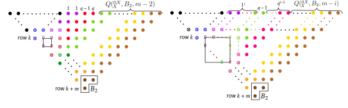
Figure 13: Left: If $\Box$ has minimal size, then Lemma 3.2.4 shows that the first of the two red entries can take any of the $q-1$ different values that would close the window. The second is free to take any value. Right: The dot diagram when the window on row $k$ is size $i$.

This contributes $q(q-1)\cdot Q(\begin{subarray}{c}\phantom{X}0X\\ X\end{subarray},B_{2},m-2)$ to the total sum. In general, if the window has size $i\times i$, it contributes $(q-1)q^{i-1}Q(\begin{subarray}{c}\phantom{X}0X\\ X\end{subarray},B_{2},m-i)$ to the total. This is illustrated in the right-hand side of Figure 13. Summing over all values of $i$ gives

$$Q(\begin{subarray}{c}\phantom{X}XX\\ X\end{subarray},B_{2},m) =(q-1)(q-2)\cdot Q(\begin{subarray}{c}\phantom{X}XX\\ X\end{subarray},B_{2},m-1)+(q-1)\cdot Q(\begin{subarray}{c}\phantom{I}X0\\ X\end{subarray},B_{2},m-1)$$

$$+(q-1)\cdot Q(\begin{subarray}{c}\phantom{X}XX\\ 0\end{subarray},B_{2},m-1)+\sum_{i=1}^{m-1}(q-1)q^{i-1}\cdot Q(\begin{subarray}{c}\phantom{X}0X\\ X\end{subarray},B_{2},m-i).$$ (3.3.2)

Note that the $Q(\begin{subarray}{c}\phantom{X}0X\\ X\end{subarray},B_{2},m-1)$ term from (3.3.1) has been absorbed into the sum above. At this point, a specific choice for $B_{2}$ is made, the induction hypothesis is used and the sum is evaluated using the geometric sequence formula to obtain relations $(1.3)$, $(2.2)$ and $(3.1)$.

The values of $Q(\begin{subarray}{c}\phantom{X}XX\\ 0\end{subarray},B_{2},m)$ and $Q(\begin{subarray}{c}\phantom{I}X0\\ X\end{subarray},B_{2},m)$ are derived using an identical method. For this reason, these proofs are omitted. ∎

These equations are put to use in the next subsection to count the number of finite sequences with a given window in their number wall.

3.4 Counting Sequences with a given Window in their Number Wall

The following definitions are made to categorise the types of windows that can appear in a finite number wall. From now on, windows are denoted by squares, such as $\Box$. A window $\Box$ with side length $l$ and top left corner in row $m$ and column $n$ is written as a triple $\Box(l,n,m)$.

Definition 3.4.1.

There are three types of windows that can appear on a finite number wall, categorised as follows:

• A window is complete if the entire window and its inner frame is contained in the number wall.

• A window in a finite number wall is closed if the ratios of the geometric sequences comprising its inner frame have all been determined. Equivalently, its size is independent of any entries added to the given sequence generating the number wall. A window is left-side closed if the ratio of the inner frame on the left side is determined. A window being right-side closed is defined similarly.

  

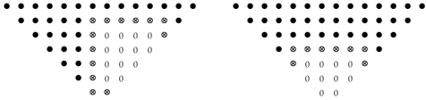
  Figure 14: Two examples of closed windows. In the second example all four ratios of the inner frames are determined by Theorem 3.1.5 .

• A window is open if it is not closed. A window being left-side open and right-side open is defined similarly. Equivalently, a window is open if it could grow in size depending what additional entries are added to the start or to the end of the generating sequence. Similarly, a window is right-side open (left-side open, respectively) if an entry added on the end (start, respectively) of the generating sequence could increase the size of the window.

  

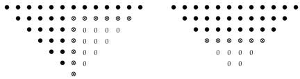
  Figure 15: Two examples of open windows. The first example is left-side closed and right-side open. The second example is both right-side and left-side open.

A complete window is closed, but a closed window is not necessarily complete. The following terminology describes the entries in a sequence that generate windows in number walls.

Definition 3.4.2.

Let $r\in\mathbb{N}$ and let $W(S)$ be the number wall of a finite sequence $S=(s_{i})_{0\leq i\leq r}$. Additionally, let $\Box$ be a window of side length $l\in\mathbb{N}$ in $W(S)$. Using the notation from Figure 1, the hat of $\Box$ is the set $\{A_{0},\dots,A_{l}\}$. That is, the hat of a window is the top row of its inner frame. The hat generator of $\Box$ is the shortest subsequence $S_{\Box}=(s_{i})_{n_{1}\leq i\leq n_{2}}\subseteq S$ such that $W(S_{\Box})$ contains the hat of the window. The hat cone of a window is the number wall generated by the hat generator.

Let $S_{\Box}=\{s_{i}\}_{1\leq i\leq k}$ be a hat generator for an open window $\Box$. Then a left-side closure of $S_{\Box}$ is defined as a sequence $\{s_{i}\}_{0\leq i\leq k}$ with $s_{0}$ chosen such that the window $\Box$ is left-side closed. A right-side closure of $s_{\Box}$ is defined similarly, as a sequence $\{s_{i}\}_{1\leq i\leq k+1}$ which makes $\Box$ right-side closed. Finally, a closure of $S_{\Box}$ is a sequence $\{s_{i}\}_{0\leq i\leq k+1}$ with $s_{0}$ and $s_{k+1}\in\mathbb{F}_{q}$ being such that the window $\Box$ is closed. By Lemma 3.2.4, $q-1$ of the possible $q$ choices for $s_{0}$ (for $s_{k+1}$, respectively) create left-side (right-side, respectively) closures.

For a window $\Box(l,n,m)$, it is clear the hat generator has length $2m+l$. Furthermore, for a sequence $S=(s_{i})_{1\leq i\leq r}$ which has $\Box(l,n,m)$ in its number wall, the hat generator is the subsequence $S_{\Box(l,n,m)}=(s_{i})_{n-m\leq i\leq n+m+l-1}$. One further entry on either side of $S_{\Box(l,n,m)}$ is required to close the window at each end and hence there cannot be a closed or complete window of size $l$ with top left corner on row $m$ and column $n$ if $r<n+m+l$ or if $n-(m+1)\leq 0$.

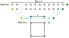
Figure 16: The hat of the window $\Box(l,n,m)$ is in blue. The grey portion of the top row is the hat generator of $\Box(l,n,m)$ and the grey and blue portions combined with $\Box(l,n,m)$ are the hat cone of $\Box(l,n,m)$. The entire top row is the closure of the hat generator, whilst the grey and light (dark, respectively) green parts of the top row are the left-side (right-side, respectively) closures of $S_{\Box(l,n,m)}$.

Theorem 1.0.5 only demands that a particular square portion of the number wall should be zero; not that the window is exactly the given size or begins exactly in the given place. This motivates the following definition:

Definition 3.4.3.

A window $\Box_{1}=\Box_{1}(l_{1},n_{1},m_{1})$ contains a window $\Box_{2}=\Box_{2}(l_{2},n_{2},m_{2})$ if $\Box_{2}$ is fully inside $\Box_{1}$. Explicitly, this occurs if and only if

$$n_{2}\geq n_{1}, n_{2}+l_{2}\leq n_{1}+l_{1}, m_{2}\geq m_{1} m_{2}+l_{2}\leq m_{1}+l_{1}.$$ and

Given a window $\Box$, the following lemma shows how many ways a number wall with nonzero right-side blade can be extended to have a window containing $\Box$.

Lemma 3.4.4.

Let $k,l,m$ be natural integers, $\Box=\Box(l,m+k,m+k+2)$ be a window and $i\in\{1,2\}$. Given a sequence $S_{k}\subset\mathbb{F}_{q}^{2k+i}$ of length $2k+i$ with a nonzero right-side blade $B$ in its number wall, there are $q^{2m+1-i}$ ways to continue it to a sequence of length $2k+1+2m+l$ so as to have a window $\Box^{\prime}$ that contains $\Box$ in the number wall of the resulting extended sequences.

Proof.

The case where $i=1$ is completed first. The diagram below illustrates the set up.

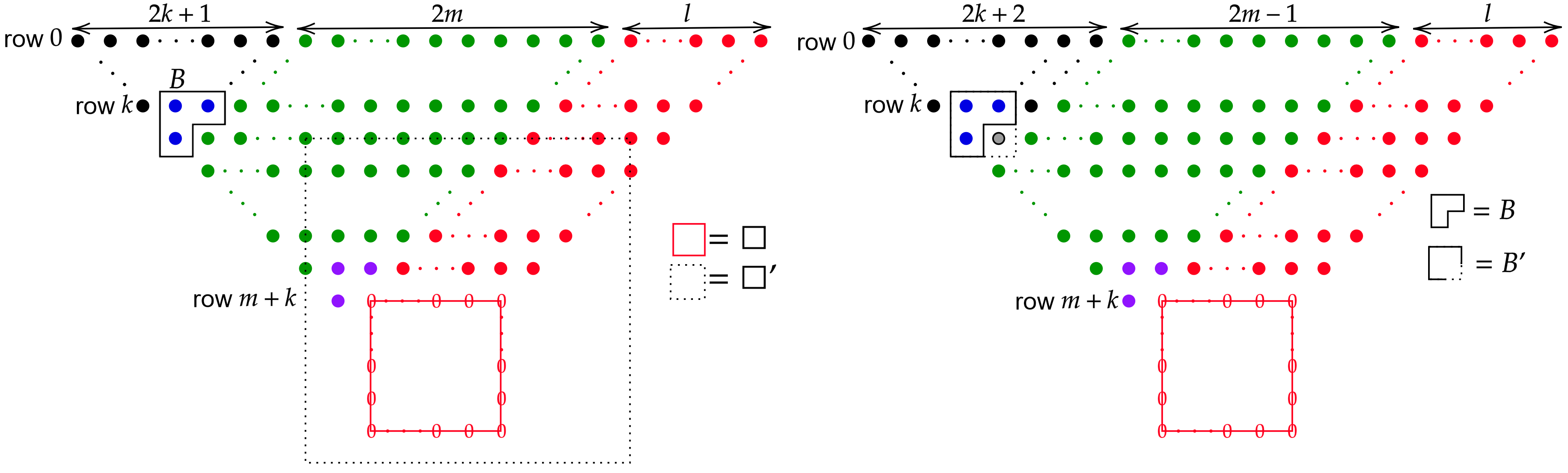
Figure 17: Left: The $i=1$ case. The sequence $S_{k}$ (top row, black) has nonzero blade (dark blue). It is extended by $2m+l$ entries (top row, light blue and red) so that the extended number wall has a window $\Box^{\prime}$ (dotted) containing the window $\Box$ (red). Here, the dotted lines mean that this is just one of many possible examples of $\Box^{\prime}$. The right-side blade of the sequence of length $2k+2m+1$ is in purple. Right: The $i=2$ case.

In this case, the result is proved by partitioning the set of all the windows containing $\Box$ by the row and column they begin in. Thus, the first section of the partition contains all the windows whose first column/row is in the same as the first column/row of $\Box$. This partition is illustrated by the left dot diagram below.

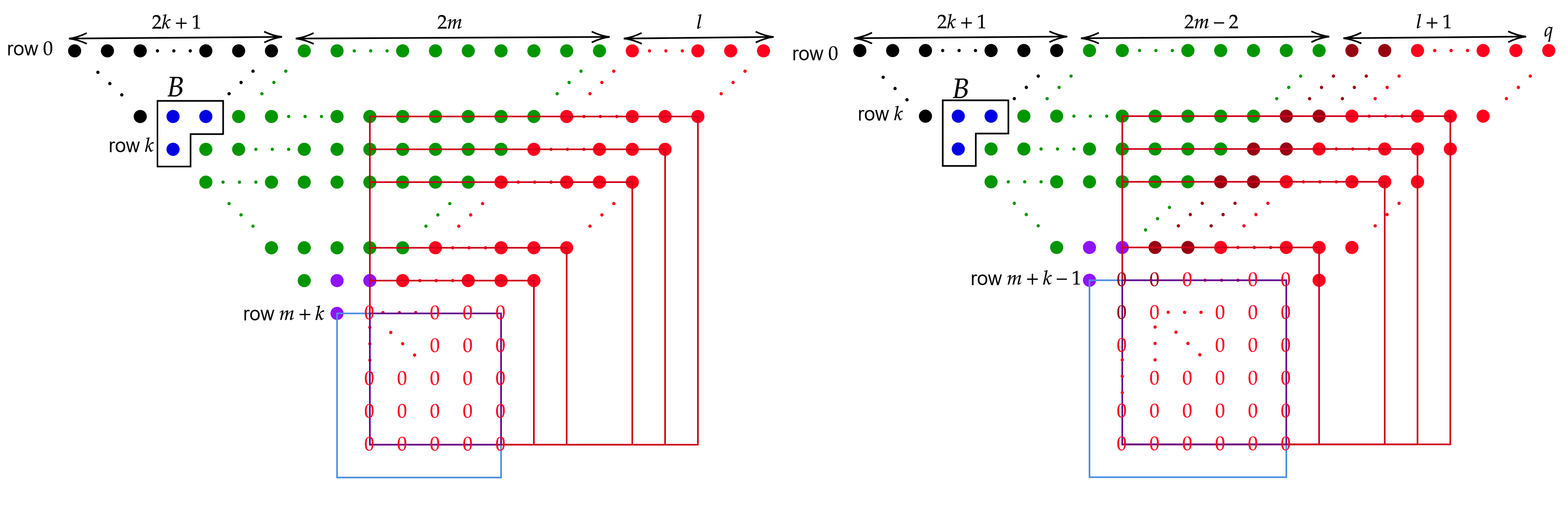
Figure 18: Left: The purple square denotes the single window which starts in the same row and column as $\Box$; that is, $\Box$ itself. The blue square represents the window that contains $\Box$ which starts on the same row as $\Box$. All the red squares represent the windows that start in the same column as $\Box$. Right: When the starting row or column has been decreased by one, the windows in this partition are one row higher. This shortens the blue sequence by two terms. The dark red entries are the ones that were in the green extension to $S_{k}$ but are now part of the unique extension required to generate the window.

With notation from Definition 3.3.3, there are $Q(B,\begin{subarray}{c}\phantom{X}XX\\ X\end{subarray},m)$ ways of obtaining the purple right side blade in the right image of Figure 18, and then Lemma 3.2.4 implies there is a unique extension of length $l$ giving the purple window. By the same method (that is, by repeated applications of Lemma 3.2.4), there are $Q(B,\begin{subarray}{c}\phantom{X}XX\\ 0\end{subarray},m)$ ways of obtaining the blue window. Each red window is counted once in the value of $Q(B,\begin{subarray}{c}\phantom{I}X0\\ X\end{subarray},m)$, and also must be extended $l$ times by applying Lemma 3.2.4. Therefore, this whole partition contributes

$$Q(B,\begin{subarray}{c}\phantom{X}XX\\ X\end{subarray},m)+Q(B,\begin{subarray}{c}\phantom{X}XX\\ 0\end{subarray},m)+Q(B,\begin{subarray}{c}\phantom{I}X0\\ X\end{subarray},m)$$

to the total sum. The next partition is similar, but contains all the windows that have first row or first column one before the first row or column of $\Box$. This is illustrated in the right-hand side of Figure 18. Similar to the previous partition, there are $qQ(B,\begin{subarray}{c}\phantom{X}XX\\ X\end{subarray},m-1)$ ways to obtain the purple window. The extra factor of $q$ is a consequence of the depth of the window being decreased by one and its size being increased by one. The decrease in depth reduces the size of the hat generator by two. However, the increase in size enlarges the size of the hat generator by one. Therefore, the hat generator has only decreased its length by one. This leaves the last entry in the sequence redundant and hence free to take any value. With a similar argument for the red and blue windows, this case contributes

$$q\big{(}Q(B,\begin{subarray}{c}\phantom{X}XX\\ X\end{subarray},m-1)+Q(B,\begin{subarray}{c}\phantom{X}XX\\ 0\end{subarray},m-1)+Q(B,\begin{subarray}{c}\phantom{I}X0\\ X\end{subarray},m-1)\big{)}$$

to the total sum. Each partition is done in a similar way, leading to a total value of

$$\sum^{m}_{i=0}q^{i}\big{(}Q(B,\begin{subarray}{c}\phantom{X}XX\\ X\end{subarray},m-i)+Q(B,\begin{subarray}{c}\phantom{X}XX\\ 0\end{subarray},m-i)+Q(B,\begin{subarray}{c}\phantom{I}X0\\ X\end{subarray},m-i)\big{)}.$$ (3.4.1)

From Lemma 3.3.4, it can be seen that for $m>1$,

$$Q(B,\begin{subarray}{c}\phantom{X}XX\\ X\end{subarray},m)+Q(B,\begin{subarray}{c}\phantom{X}XX\\ 0\end{subarray},m)+Q(B,\begin{subarray}{c}\phantom{I}X0\\ X\end{subarray},m)=q^{2m-1}(q-1).$$ (3.4.2)

If $B=\begin{subarray}{c}\phantom{X}XX\\ X\end{subarray},\begin{subarray}{c}\phantom{I}X0\\ X\end{subarray},$ or $\begin{subarray}{c}\phantom{X}XX\\ 0\end{subarray}$, this formula also applies for $m=1$ and the sum equals 1 for $m=0$. If $B=\begin{subarray}{c}\phantom{X}0X\\ 0\end{subarray},\begin{subarray}{c}\phantom{X}0\phantom{i}0\\ X\end{subarray}$ or $\begin{subarray}{c}\phantom{X}0X\\ X\end{subarray}$ then at $m=1$, the left-hand side of (3.4.2) has value $q^{2}$.

In the former case when $B=\begin{subarray}{c}\phantom{X}XX\\ X\end{subarray},\begin{subarray}{c}\phantom{I}X0\\ X\end{subarray}$ or $\begin{subarray}{c}\phantom{X}XX\\ 0\end{subarray}$,

$$(\ref{containtotal}) =\sum_{j=0}^{m-1}q^{2m-1-2j}(q-1)\cdot q^{j}+q^{m}=q^{m}((q-1)(q^{m-1}+q^{m-2}+\dots+q+1)+1)=q^{2m}.$$

In the latter case when $B=\begin{subarray}{c}\phantom{X}0\phantom{i}0\\ X\end{subarray},\begin{subarray}{c}\phantom{X}0X\\ 0\end{subarray},$ or $\begin{subarray}{c}\phantom{X}0X\\ X\end{subarray}$,

$$(\ref{containtotal}) =\sum_{j=0}^{m-2}q^{2m-1-2j}(q-1)\cdot q^{j}+q^{m-1}\cdot q^{2}=q^{m+1}((q-1)(q^{m-2}+q^{m-3}+\dots+q+1)+1)=q^{2m}.$$

This proves the lemma in the $i=1$ case. Most of the hard work for the $i=2$ case has already been done. The right-side diagram of Figure 17 illustrates the set up. If the bottom right entry of $B^{\prime}$ (grey interior in the figure) is nonzero, then the right side blade created by adding any of the $q$ elements of $\mathbb{F}_{q}$ to $S^{\prime}_{k}$ is necessarily nonzero. Hence, there are $q^{2m-2}$ continuations giving a window containing $\Box$ (by the $i=1$ case). If the bottom right entry is zero, the right-side blade $B$ (boxed part of $B^{\prime}$) must be nonzero since $B^{\prime}$ is nonzero and the bottom right entry of $B^{\prime}$ is zero. Furthermore, as the bottom right entry is zero, this implies that $B$ is either $\begin{subarray}{c}\phantom{X}XX\\ X\end{subarray},\begin{subarray}{c}\phantom{I}X0\\ X\end{subarray}$ or $\begin{subarray}{c}\phantom{X}XX\\ 0\end{subarray}$. The $i=1$ case shows there are $q^{2m}$ continuations of a sequence of length $2k+1$ with right-side blade $B$. These continuations are partitioned into those that have zero in bottom right position in $B^{\prime}$ and those that do not. In the latter case, Lemma 3.2.4 shows the number of continuations with a window containing $\Box$ is $(q-1)q^{2m-1}$. Hence, there are $q^{2m}-(q-1)q^{2m-1}=q^{2m-1}$ continuations when the bottom right entry is zero. This concludes the proof. ∎

Lemma 3.4.4 is used to prove the following corollary:

Corollary 3.4.5.

Let $q$ be a prime power, $r,n,m,l$ be natural numbers with $r\geq 2m+1+l$ and $\Box=\Box(l,n,m)$ be a window in a number wall over $\mathbb{F}_{q}$. The number of sequences of length $r$ over $\mathbb{F}_{q}$ whose number wall has a window containing $\Box$ is $q^{r-l}$.

Proof.

Since row $-1$ is made of entirely 1s, a sequence of length 1 can only have two possible right-side blade shapes. Namely, the possible blades are $\begin{subarray}{c}\phantom{X}XX\\ X\end{subarray}$ ($q-1$ ways) or $\begin{subarray}{c}\phantom{X}XX\\ 0\end{subarray}$ ($1$ way). An additional $2m+l$ entries are required to create the desired window on row $m$. Using Lemma 3.4.4, each of these two blades have $q^{2m}$ possible continuations that give a window containing $\Box$. This gives a total of

$$(q-1)\cdot q^{2m}+1\cdot q^{2m}=q^{2m+1}$$

sequences of length $2m+l+1$ that have the desired window. The remaining choices for the sequence are free, giving a total number of sequences of length $r$ as

$$q^{r-2m-1-l}\cdot q^{2m+1}=q^{r-l}.$$

This concludes the proof. ∎

Lemma 3.4.4 demands that the finite number wall has a nonzero right-side blade. The following lemma deals with the complementary case where the right-side blade is the zero blade.

Lemma 3.4.6.

Let $k,m\in\mathbb{N}$, $i\in\{1,2\}$ and $\Box^{\prime}=\Box^{\prime}(l,m+k,m+k+2)$ be a window. Given a sequence $S_{k}\subset\mathbb{F}_{q}^{2k+i}$ of length $2k+1$ with the zero right-side blade in its number wall, there are $q^{2m+1-i}$ ways to extend $S_{k}$ to a sequence of length $2k+2m+l+1$ so as to have a window that contains $\Box^{\prime}$ in their number wall.

Proof.

Let $\Box$ be the window containing the zero blade of the number wall of $S_{k}$. Assume that $\Box$ is closed (see Definition 3.4.1). The diagram on the left below illustrates the scenario.

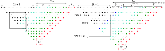
Figure 19: Left: The sequence $S_{k}$ is in black, and $\Box$ is the window containing the right-side blade. Right: The first possible closure if $\Box$ is open.

Define $s$ as the vertical distance from the number wall generated by the inner frame of $S_{k}$ to the bottom of the deepest right-side blade determined by $\Box$. Note that if $S_{k}$ has odd length then $s$ is even, and if $S_{k}$ has even length, then $s$ is odd. When $S_{k}$ is continued by $s$ entries, coloured in light blue in Figure 19, the right-side blade of the number wall is independent of the choice of continuation, as the right-side blade is in the inner frame of $\Box$. The conditions of Lemma 3.4.4 are now satisfied, and hence there are $q^{2m-s}$ continuations in the odd case (and $q^{2m-1-s}$ in the even case) from this blade to get a window containing $\Box^{\prime}$. Multiplying by any of the $q^{s}$ continuations of $S_{k}$ concludes the proof of the closed case.

Now assume $\Box$ is open and that $S_{k}$ has odd length. As the sequence $S_{k}$ is extended, $\Box$ is either closed or continued. For each digit added, there are $q-1$ choices to close the window and only one choice to continue it. The proof amounts to summing over every possible size the window $\Box$ could have when it is closed. Define $u\in\mathbb{N}$ such that $\Box$ starts on row $k-u$ and $v\in\mathbb{N}$ such that row $k+v$ contains the bottom row of $\Box$. Then the open window $\Box$ has size $u+1+v$. Assume $\Box$ is extended by $j$ entries so it has size $j+u+v+1$. This is illustrated in the right-side diagram of Figure 19. The dark blue entry has $q-1$ possible choices, as it closes the window $\Box$. The problem has now reduced to the closed case, and hence this case contributes

$$(q-1)\cdot q^{2v+1+j}\cdot q^{2m-2v-2-2j}=(q-1)\cdot q^{2m-1-j}$$ (3.4.3)

to the sum. This ends when $2m-2v-2-2j=2$, that is, when $j=m-v-2$. There is one final term of the sum that has not been considered, represented by the number wall where the size of $\Box$ increased so that $\Box$ contains $\Box^{\prime}$. This is illustrated below:

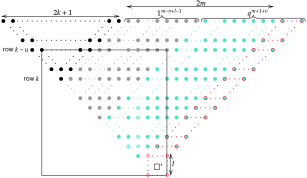
Figure 20: The dot diagram when window $\Box$ now contains $\Box^{\prime}$. The entries that were chosen uniquely to create $\Box^{\prime}$ (red in Figure 19) can now be chosen arbitrarily.

The size of $\Box$ has increased by $l+1$ from the case $j=m-v-2$. As the closing coefficient is no longer required (because $\Box^{\prime}$ is contained inside of $\Box$), there is now $q^{m+1+v}$ continuations of $S_{k}$ of length $2m+l$. Hence, the total sum is

$$q^{m+1+v}+\sum_{j=0}^{m-v-2}(q-1)\cdot q^{2m-1-j}=q^{2m}.$$ (3.4.4)

This proves the result in the odd case. In the even case, the first term of the sum in (3.4.4) is ignored. Repeating the calculation completes the proof. ∎

A final definition formalises the idea of two windows ‘touching’:

Definition 3.4.7.

Let $\Box$ be a window inside a given portion of number wall, and let $\Box^{\prime}$ be another window in the number wall. Then $\Box$ undershoots $\Box^{\prime}$ if $\Box$ and its inner frame do not intersect $\Box^{\prime}$. If the inner frame of $\Box$ intersects $\Box^{\prime}$, then $\Box$ hits $\Box^{\prime}$ and $\Box$ and $\Box^{\prime}$ cannot be on the same number wall. Finally, if $\Box$ contains $\Box^{\prime}$, or if $\Box$ intersects $\Box^{\prime}$ and can be extended to contain $\Box^{\prime}$, then $\Box$ overshoots $\Box^{\prime}$.

These definitions are illustrated below.

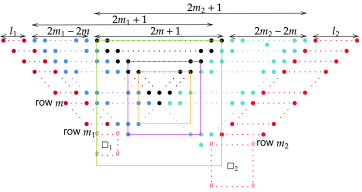
Figure 21: The green window overshoots $\Box_{1}$ and $\Box_{2}$, as it is right-side open so can be extended to contain $\Box_{2}$. The purple window being left-side closed means it hits $\Box_{1}$. However, as the purple window is right-side open, it overshoots $\Box_{2}$. The orange window undershoots both $\Box_{1}$ and $\Box_{2}$.

The combinatorics on Number Walls needed to establish Theorem 1.0.7 has been developed.

4 Hausdorff Dimension of the Set of Counterexamples to $t$-LC with Additional Growth Function

For a set $X\subset\mathbb{F}_{q}((t^{-1}))$, define the diameter of $X$ as

$$\textup{diam}(X)=\sup\{|x-y|:x,y\in X\}.$$

The following classical theorem from [9] is used to attain the lower bound for the Hausdorff dimension in Theorem 1.0.7.

Lemma 4.0.1 (Mass Distribution Principle).

Let $\mu$ be a probability measure supported on a subset X of $\mathbb{F}_{q}((t^{-1}))$. Suppose there are positive constants $a$, $s$ and $l_{0}$ such that

$$\mu(B)\leq a\cdot\textup{diam}(B)^{s}$$

for any ball $B$ with size $\textup{diam}(B)\leq l_{0}$. Then $\dim(X)\geq s$.

Proof of Theorem 1.0.7.

Recall the set $M(f,t)$ from Definition 1.0.11. Theorem 1.0.5 shows that if a Laurent series $\Theta(t)$ is in $M(f,t)$, then there exists an $l\in\mathbb{N}$ such that for any $k\in\mathbb{N}$, the windows with top left corner on the $k^{\textup{th}}$ column of the number wall generated by $\Theta(t)$ have size less than or equal to $l+\lceil\log_{q}(f(q^{k}))\rceil-1$. For the duration of this proof, a sequence satisfying this property in the size of its windows as $k$ tends to infinity is said to satisfy the window growth property with respect to function $f$. The strategy of the proof is to construct a Cantor set of sequences with number walls satisfying this window growth property; it is shown to have full dimension.

Let $\mathcal{J}_{n}$ be the set of balls $J_{n}$ generated by a sequence of length $q^{n}$ whose number wall has windows satisfying the window growth property with respect to function $f$. The goal is to construct $\mathcal{J}_{n+1}$. To do this, each $J_{n}\in\mathcal{J}_{n}$ is split into $R_{n}:=q^{(q^{n+1}-q^{n})}$ sub-cylinders, each generated by a sequence of length $q^{n+1}$. These $R_{n}$ sequences collectively make the set $\mathcal{I}_{n+1}$. Every sequence in $\mathcal{I}_{n+1}$ that has a window of size larger than $l+\lceil\log_{q}(f(q^{k}))\rceil-1$ starting on column $k$ needs to be removed.

To begin, it is sufficient to remove all sequences with a window of size $l+\lceil\log_{q}(f(q^{k}))\rceil-1$ on diagonal $k$ instead of column $k$. Indeed, every entry on diagonal $k$ is in column at least $\frac{k}{2}$. Therefore, for each diagonal, removing all windows of size $l+\lceil\log_{q}(f(q^{\frac{k}{2}}))\rceil-1$ is sufficient. When $f=\log^{2}$, this equals $l+\lceil\log_{q}(k^{2})+\log_{q}\left(\frac{1}{4}\right)\rceil-1$. The constant $\lceil\log_{q}\left(\frac{1}{4}\right)\rceil$ is absorbed into $l$, which can be any fixed natural number.

The proof proceeds by induction, with the base case being any sequence of length 1. As the number wall generated by the first $q^{n}$ entries already satisfies the window growth property with respect to function $f$ by induction, only the windows on diagonals $q^{n}<k\leq q^{n+1}$ are checked. This is illustrated by the following dot diagram:

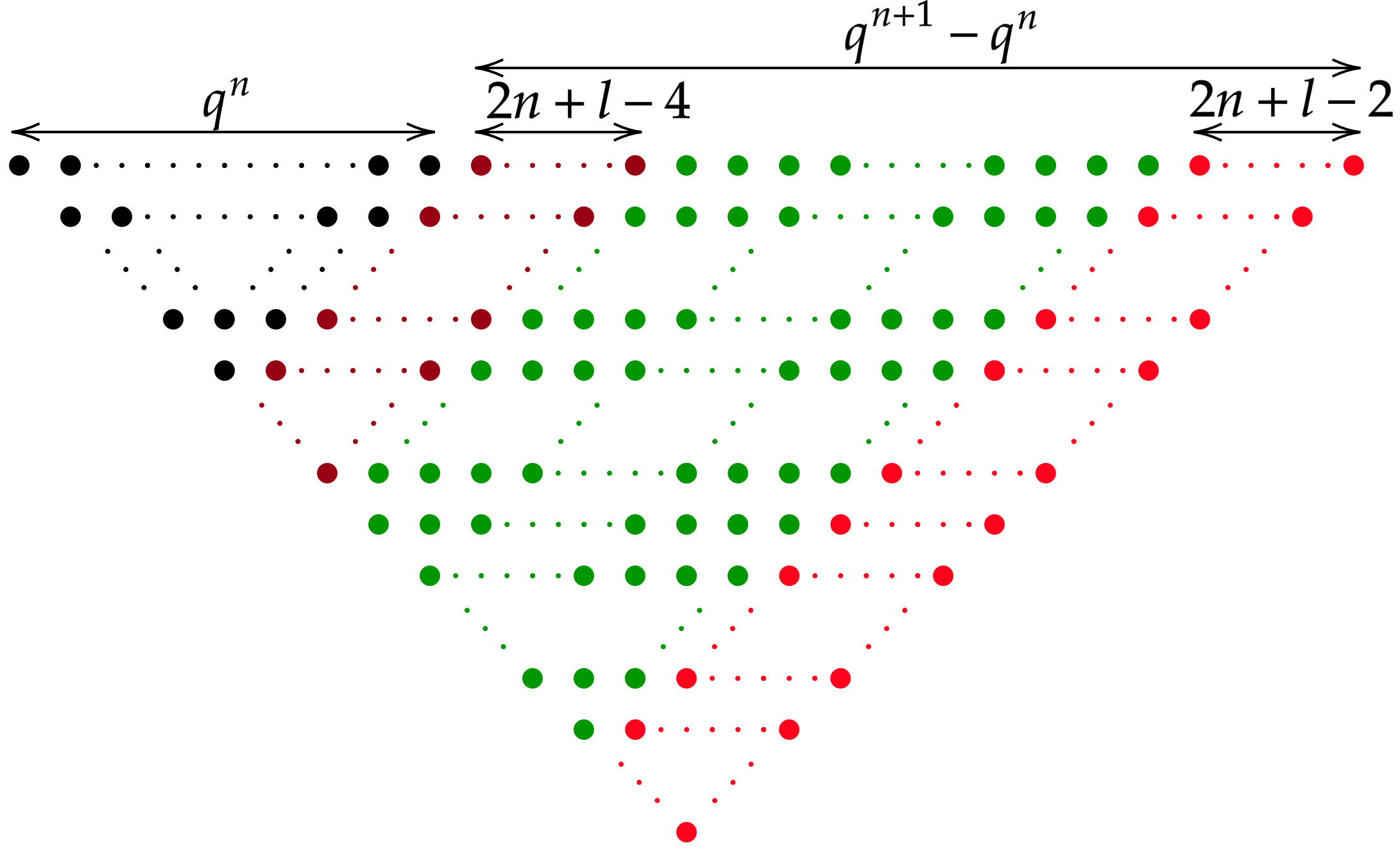
Figure 22: The black dots represent the number wall generated by the cylinder $J_{n}$. The rest of the colours are the number wall generated by some extension $I_{n}$.

If a position in the number wall of $I_{n}$ is undershot by a window from the number wall of $J_{n}$, then Lemma 3.4.6 shows there are

$$R_{n}\cdot q^{-(l+\lceil\log_{q}(k^{2})\rceil-1)}\leq R_{n}\cdot q^{-(l+2n-1)}$$

continuations that contain a window of problematic size in that position. Since every sequence in $J_{n}$ satisfies the window growth property, any position denoted in green in Figure 22 will not be overshot by any window in $J_{n}$. The positions denoted in dark red could be overshot, but are not necessarily, so it is not difficult to see that the number of positions in the extended number wall that a window could begin in is bounded above by $q^{2n+2}$. Hence, the amount to be thrown away from the green and red bands combined in Figure 22 is less than or equal to

$$R_{n}\cdot q^{2n+2-(l+2n-1)}=R_{n}\cdot q^{3-l}.$$ (4.0.1)

This represents all the positions that are undershot by a window in $J_{n}$. The bands coloured in red and brown in Figure 22 are more problematic. Entries in the brown band could be overshot by windows from $J_{n}$. Note, the red band will be directly adjacent to the brown band of the next level set. For this reason, the light red band is dealt with first.

For ease, define $L:=l+2n-1$, the size of problematic windows, and let $l$ be odd and sufficiently large. In the first diagonal on the light red band, each position is removed from the Cantor set if it has a window of size $L-1$. Lemma 3.4.6 shows there are $R_{n}\cdot q^{-L+1}$ extensions giving this, and there are less than $q^{n+1}$ such positions. Similarly for the second diagonal, all windows of size $L-2$ are thrown away. This continues until diagonal $L/2$, where all the windows of size $L/2$ are thrown away. Nothing is thrown away from the remaining diagonals. This leads to a total removal of

$$R_{n}\cdot q^{n+1}\cdot q^{-L/2}(q^{-L/2-1}+\dots+1)\ll_{q}R_{n}\cdot q^{n+1-L/2}=R_{n}\cdot q^{1-(l-1)/2}.$$ (4.0.2)

The dark red band is now dealt with. As previously noticed, this is directly adjacent to the light red band of the previous level set. Therefore, by induction, only entries in the first $L/2-1$ diagonals could be overshot. There are $q^{n}$ such entries in the first diagonal, and at most

$$R_{n}\cdot q^{-L/2}$$ (4.0.3)

sequences are thrown away (in the case where the position is overshot by a window from $J_{n}$). For an entry in the second diagonal, there are two cases. It is either part of an open window or a closed window. The first case has already been removed, as it would necessarily be part of an open window on the first diagonal. Nothing is removed in the second case, as the window is closed and smaller than the problematic size.

Combining equations (4.0.1), (4.0.2) and (4.0.3) shows that the number of extensions that satisfy the window growth rate is bounded below by

$$t_{n}(l):=R_{n}\left(1-q^{3-l}-D_{q}q^{-l/2}\right)$$ (4.0.4)

for some constant $D_{q}$ depending only on $q$, coming from the implicit constant in (4.0.2). If $l$ is sufficiently large, $t_{n}(l)$ is always positive. Define then

$$r_{n}:=R_{n}\cdot\left(q^{3-l}-D_{q}q^{-l/2}\right).$$

Let $\mathbf{K}(\mathbb{I},\mathbf{R},\mathbf{r})$ be a Cantor set with $\mathbf{R}=(R_{n})_{n\geq 0}$ and $\mathbf{r}=(r_{n})_{n\geq 0}$: it is constructed by starting with the unit interval and splitting each level set into $R_{n}$ sub-balls and throwing at most $r_{n}$ of them away. Let $\varepsilon>0$ be small. Then there exists some $n_{0}\in\mathbb{N}$ depending on $\varepsilon$ such that for all $n>n_{0}$

$$R_{n}^{1-\varepsilon}\leq t_{n}(l),$$ (4.0.5)

which is true for $l$ large enough. The remainder of this proof is similar to an argument made by Badziahin and Velani in [17, Lemma 1]. A probability measure $\mu$ is defined on $\mathbf{K}(\mathbb{I},\mathbf{R},\mathbf{r})$ recursively: For $n=0,$ set

$$\mu(J_{0}):=1.$$

For $n\geq 1,$ let

$$\mu(J_{n}):=\frac{\mu(J_{n-1})}{\#\{J\in\mathcal{J}_{n}:J\subset J_{n-1}\}},$$ (4.0.6)

where $J_{n-1}\in\mathcal{J}_{n-1}$ is the unique interval such that $J_{n}\subset J_{n-1}$. It is shown in [9, Proposition 1.7] that $\mu$ can be extended to all Borel sets $F$ of $\mathbb{F}_{q}((t^{-1}))$ by

$$\mu(F):=\mu(F\cap\mathbf{K}(\mathbb{I},\mathbf{R},\mathbf{r})=\inf\left\{\sum_{J\in\mathcal{J}}\mu(J)\right\},$$

where the infimum is over all coverings $\mathcal{J}$ of $F\cap\mathbf{K}(\mathbb{I},\mathbf{R},\mathbf{r})$ by intervals $J\in\{\mathcal{J}_{n}:n\geq 0\}.$ For any interval $J_{n}\in\mathcal{J}_{n}$, (4.0.6) and the definition of $t_{n}(l)$ in (4.0.4) implies that

$$\mu(J_{n})\leq t_{n-1}^{-1}\mu(J_{n-1}).$$

Inductively, this yields

$$\mu(J_{n})\leq\prod_{i=0}^{n-1}t^{-1}_{i}.$$ (4.0.7)

Next, let $\delta_{n}$ denote the length of a generic interval $J_{n}\in\mathcal{J}_{n}$. It is clear that

$$\delta_{n}=\prod_{i=0}^{n-1}R_{i}^{-1}.$$ (4.0.8)

For any arbitrary ball $C\subset\mathbb{I}$ satisfying $\textup{diam}(C)\leq\delta_{n_{0}}$, there exists an integer $n\geq n_{0}$ such that

$$\delta_{n+1}\leq\textup{diam}(C)<\delta_{n}.$$ (4.0.9)

Hence,

$$\mu(C) \leq\sum_{\begin{subarray}{c}J\in\mathcal{J}_{n+1}\\ J\cap C\neq\emptyset\end{subarray}}\mu(J)\leavevmode\nobreak\ \leavevmode\nobreak\ \leavevmode\nobreak\ \begin{subarray}{c}(\ref{Cantor3})\\ \leq\end{subarray}\leavevmode\nobreak\ \leavevmode\nobreak\ \leavevmode\nobreak\ \left(\frac{\textup{diam}(C)}{\delta_{n+1}}\right)\left(\prod_{i=0}^{n}t^{-1}_{i}\right)\leavevmode\nobreak\ \leavevmode\nobreak\ \leavevmode\nobreak\ \begin{subarray}{c}(\ref{Cantor4})\\ =\end{subarray}\leavevmode\nobreak\ \leavevmode\nobreak\ \leavevmode\nobreak\ \textup{diam}(C)^{\varepsilon}\left(\prod_{i=0}^{n}\frac{R_{i}}{t_{i}}\right)\cdot\textup{diam}(C)^{1-\varepsilon}$$

$$\begin{subarray}{c}(\ref{Cantor5})\\ <\end{subarray}\left(\delta_{n}\right)^{\varepsilon}\cdot\left(\prod_{i=0}^{n}\frac{R_{i}}{t_{i}}\right)\cdot\textup{diam}(C)^{1-\varepsilon}\leavevmode\nobreak\ \leavevmode\nobreak\ \leavevmode\nobreak\ \begin{subarray}{c}(\ref{Cantor4})\\ =\end{subarray}\leavevmode\nobreak\ \leavevmode\nobreak\ \leavevmode\nobreak\ \frac{R_{n}}{t_{n}}\left(\prod_{i=1}^{n-1}\frac{R_{i}^{1-\varepsilon}}{t_{i}}\right)\cdot\textup{diam}(C)^{1-\varepsilon}.$$ (4.0.10)

Using that $d:=\frac{R_{n}}{t_{n}}$ is a constant depending only on the fixed number $l$,

$$(\ref{Cantor 6})\leavevmode\nobreak\ \leavevmode\nobreak\ \leavevmode\nobreak\ \begin{subarray}{c}(\ref{cantor1})\\ <\end{subarray}\leavevmode\nobreak\ \leavevmode\nobreak\ \leavevmode\nobreak\ d\cdot\prod_{i=1}^{n_{0}}\frac{R_{i}^{1-\varepsilon}}{t_{i}}\cdot\textup{diam}(C)^{1-\varepsilon}.$$

Hence, by the Mass Distribution Principle (Lemma 4.0.1), $\mathbf{K}(\mathbb{I},\mathbf{R},\mathbf{r})$ has dimension greater than or equal to $1-\varepsilon$ for any $\varepsilon>0$. Therefore, $\mathbf{K}(\mathbb{I},\mathbf{R},\mathbf{r})$ has dimension 1. This completes the proof. ∎

5 Structures of Zero Patterns in Number Walls

The goal is now to prove Theorem 1.0.6. To this end, recall that Corollary 3.4.5 counts how many sequences have a given square zero portion in their number wall. Two generalisations of this corollary are proved, which replace the square zero portion with one of any connected shape, or two disconnected square zero portions, respectively.

5.1 Rectangular Zero Portions

Whilst windows are always in a square shape, determining how many finite sequences have a square window that contains a given rectangular portion is essential for proving Theorem 1.0.6. To this end, the following definition is made:

Definition 5.1.1.

Let $r,n,m,l\in\mathbb{N}$, $d\in\mathbb{Z}$ satisfying $d<l$ and let $q$ be a prime power. Define $R^{l,d,n,m}_{q,r}$ as the set of sequences of length $r$ over $\mathbb{F}_{q}$ whose number wall contains a rectangular portion of zeros with horizontal length $l$, height $l-d$ and top left corner in column $n$ and row $m$.

The cardinality of $R^{l,d,n,m}_{r,q}$ can be explicitly determined:

Lemma 5.1.2.

Let $r,n,m,l\in\mathbb{N}$, $d\in\mathbb{Z}^{+}$ satisfying $0<d<l-1$ and let $q$ be a prime power. Assume at least one of the longest sides of the rectangle defined by $R^{l,d,n,m}_{q,r}$ is contained fully on the number wall. Then,

1. If $m-n\leq d\leq 0$,

   $$\#R^{l,d,n,m}_{r,q}=\frac{q^{r-l-2m-1}}{q+1}\left((-d+1)\cdot q^{2m+2}-(-d-1)\cdot q^{2m+1}-d\cdot(q-1)\right).$$ (5.1.1)

2. If $0\leq d\leq m$,

   $$\#R^{l,d,n,m}_{r,q}=\frac{q^{r-l-2m}}{(q+1)^{2}}\cdot\left((d+1)\cdot q^{2m+2}+2\cdot q^{2m+1}-(d-1)\cdot q^{2m}-q^{2d}+1\right).$$ (5.1.2)

3. If $d>m$, then equation (5.1.2) holds upon replacing $d$ with $m$ in the right-hand side.

Proof.

Equations (5.1.1) and (5.1.2) are proved by induction on $d$. When $d=0$, Lemma 5.1.2 reduces to Corollary 3.4.5, proving both base cases. Assume first that $m-n\leq d<0$. For the inductive step, let $S$ be a sequence in $R^{l,d,n,m}_{r,q}$. Then, there are three possibilities:

1. $S\in R^{l,d+1,n-1,m}_{r,q}$ and $S\not\in R^{l,d+1,n,m}_{r,q}$.

2. $S\not\in R^{l,d+1,n-1,m}_{r,q}$ and $S\in R^{l,d+1,n,m}_{r,q}$.

3. $S\in R^{l,d+1,n-1,m}_{r,q}$ and $S\in R^{l,d+1,n,m}_{r,q}$.

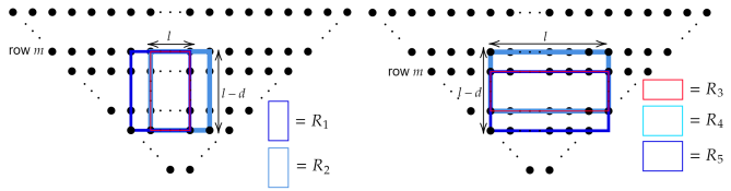
Figure 23: Left: When $d<0$, the sequences in $R^{l,d,n,m}_{r,q}$ have the red rectangle in their number wall. The sequences in case (1.1) above have a window containing $R_{1}$ and not $R_{2}$ in their number wall. Similarly, if a sequence is in case (1.2), its number wall has a window containing $R_{2}$ and not $R_{1}$. If a sequence is in case (1.3), it has a single window containing both $R_{1}$ and $R_{2}$. Right: When $d>0$, the sequences in $R^{l,d,n,m}_{r,q}$ have the red rectangle $R_{3}$ in their number wall. This means the number walls either have a window containing only $R_{4}$, only $R_{5}$ or both.

If $S$ is in case (1.3), then $S\in R^{l,d+2,n-1,m}_{r,q}$. Also, the number of sequences in case (1.1) is

$$\#R^{l,d+1,n-1,m}_{r,q}-\#R^{l,d+2,n-1,m}_{r,q}.$$

Similarly, the number of sequences in case (1.2) is

$$\#R^{l,d+1,n,m}_{r,q}-\#R^{l,d+2,n-1,m}_{r,q}.$$

Summing over the three cases gives the formula

$$\#R^{l,d,n,m}_{r,q}=\#R^{l,d+1,n-1,m}_{r,q}+\#R^{l,d+1,n,m}_{r,q}-\#R^{l,d+2,n-1,m}_{r,q}.$$

Using the induction hypotheses and doing some simple algebra completes the proof. Note that, if the top right corner of the desired rectangle is on the right-most diagonal (or the top left corner on the left-most diagonal) of the finite number wall, this method fails. However, in this case the desired rectangle is square and consequently the problem reduces to Corollary 3.4.5.

As the method is fundamentally identical, an abridged version of the proof of the case $0<d\leq m$ is now completed. By the same method as in the $d<0$ case,

$$\#R^{l,d,n,m}_{r,q}=\#R^{l,d-1,n,m}_{r,q}+\#R^{l,d-1,n,m-1}_{r,q}-\#R^{l,d-2,n,m-1}_{r,q}.$$ (5.1.3)

This is illustrated by the right-side diagram of Figure 23. Substituting the induction hypothesis into (5.1.3) and doing the necessary algebra completes the proof of (5.1.2).

Finally, suppose $d>m$ and let $R_{6}$ be the rectangle starting in column $n$ and row $m$ with width $l$ and height $l-d$. This implies that the $d-m$ rows underneath $R_{6}$ are also zero. This is illustrated below:

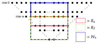
Figure 24: The difference in the height and width of $R_{6}$ (red) is greater than its starting depth. The window $W_{5}$ (blue) starts on row 0 and contains $R_{6}$. The green dotted rectangle $R_{7}$ shows the rows which must be contained in any window containing $R_{6}$.

The Square Window Theorem (Theorem 3.1.3) implies $R_{6}$ must be fully contained in a single square window. Furthermore, the window must have side lengths greater than or equal to $l$. As a window cannot start higher than row zero, there are no windows that contain $R_{6}$ that do not also contain $R_{7}$; namely, the additional $m-d$ rows underneath $R_{6}$. The difference between the width and height of $R_{7}$ is $m$, reducing the question to the previous case. This concludes the proof. ∎

Corollary 3.4.5 and Lemma 5.1.2 provide a complete picture for counting how many finite sequences have a window containing any connected portion of zeros in their number wall. Even if the portion of zeros is not in a rectangular shape, a minimally sized rectangle can be drawn around it and the Square Window Theorem (Theorem 3.1.3) shows that this rectangle is also fully zero. The next subsection extends the results of this one to count the number of sequences that have windows containing two given windows in their number wall. This is much more challenging and in some cases only an upper bound will be found. To this end, the following immediate corollary to Lemma 5.1.2 is stated for future reference:

Corollary 5.1.3.

Let $l\in\mathbb{N}$ and $d\in\mathbb{Z}$. Then

$$\#R_{r,q}^{l,d,n,m}\ll_{q}|d|\cdot q^{r-l}.$$

5.2 Pairs of Windows

This subsection provides the final result needed to prove Theorem 1.0.6. Given windows $\Box_{1}=\Box(l_{1},n_{1},m_{1})$ and $\Box_{2}=\Box(l_{2},n_{2},m_{2})$, define the set $W_{r,q}^{\Box_{1},\Box_{2}}$ as all the sequences of length $r$ over $\mathbb{F}_{q}$ whose number wall has windows that contain $\Box_{1}$ and $\Box_{2}$. The following theorem is the main result of this subsection:

Theorem 5.2.1.

Let $\Box_{1}=(l_{1},n_{1},m_{1})$ and $\Box_{2}=(l_{2},n_{2},m_{2})$ be non-overlapping windows of length $l_{1}$ and $l_{2}$ with top left entries in positions $(n_{1},m_{1})$ and $(n_{2},m_{2})$, respectively. Furthermore, let $r$ be a suitably large natural number. Then,

$$\#W_{r,q}^{\Box_{1},\Box_{2}}\ll_{q}q^{r-l_{1}-l_{2}}.$$

The proof shows this bound is sharp in many cases. If $\Box_{1}$ and $\Box_{2}$ overlap, the statement reduces to Corollary 5.1.3 from the square Window Theorem (Theorem 3.1.3). The remainder of this subsection is devoted to proving Theorem 5.2.1.

Proof of Theorem 5.2.1.

Let $i\in\{1,2\}$. The proof is split into three distinct cases, depending on how much the hat cones of $\Box_{1}$ and $\Box_{2}$ intersect. Case 1 is swiftly dealt with, but Cases 2 and 3 are split into sub-cases ((2.1), (2.2), (3.1) and (3.2)) depending on the relative positions of $\Box_{1}$ and $\Box_{2}$. Where necessary, these sub-cases are once again split into sub-sub-cases.

Case 1:

In this case, the hat cones of $\Box_{1}$ and $\Box_{2}$ do not intersect. Let $d$ be the distance between the hat cones of $\Box_{1}$ and $\Box_{2}$.

From the original definition of a number wall (Definition 3.1.2), the Toeplitz matrices making up $\Box_{1}$ and $\Box_{2}$ and their respective hat cones share no entry. Hence, Corollary 3.4.5 can be applied twice to show there are $q^{2m_{1}+1}$ choices for the $2m_{1}+1+l_{1}$ entries in the hat generator of $\Box_{1}$, and similarly for $\Box_{2}$. The rest of the sequence is filled in arbitrarily, since the desired windows have been obtained and hence any choice for the remaining entries can only increase the size of the windows. Hence there are exactly

$$q^{2m_{1}+1}\cdot q^{2m_{2}+1}\cdot q^{d}\cdot q^{r-2m_{1}-1-l_{1}-2m_{2}-l_{2}-1-d}=q^{r-l_{1}-l_{2}}$$

such sequences.

Case 2:

In this case the hat cones of $\Box_{1}$ and $\Box_{2}$ intersect but neither is contained fully in the other. Let $m$ be the depth of the intersection.

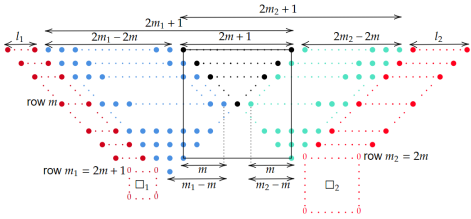
Figure 25: The intersection of the hat cones of $\Box_{1}$ and $\Box_{2}$ is in black. The portions of the hat cone that uniquely generate the window are in red and the remainder of the hat cones are in blue. The black box denotes the largest possible window contained fully in the intersection, used in Case (2.1).

There are two sub-cases to consider. In each, $r$ is taken to be the minimum value such that the windows $\Box_{1}$ and $\Box_{2}$ are able to appear on some number wall generated by a sequence of length $r$. As seen in Figure 25, $r=2m_{1}+2m_{2}-2m+l_{1}+l_{2}+1$.

Case 2.1: $m_{1}\geq 2m$ or $m_{2}\geq 2m$.

Without loss of generality, assume $m_{1}\geq 2m$. Corollary 3.4.5 shows there are $q^{2m_{2}+1}$ sequences of length $2m_{2}+1+l_{2}$ that have a window containing $\Box_{2}$ in the number wall. The goal is to show there are $q^{2m_{1}-2m}$ extensions that generate a finite number wall containing both $\Box_{1}$ and $\Box_{2}$. Taking this for granted, there are

$$q^{2m_{2}+1}\cdot q^{2m_{1}-2m}=q^{r-l_{1}-l_{2}}$$

satisfactory sequences. To prove the claim on the number of extensions, note that the largest possible window contained fully in the intersection, denoted $\Box$ (in black in Figure 25), has size $2m+1$ if the intersection has odd length, or $2m+2$ if it has even length. The horizontal distance between the column of $\Box_{1}$ closest to the intersection and the lowest point of the intersection is $m_{1}-m$. There are two sub-cases.

• If $m_{1}>2m$, there is always at least one column between $\Box_{1}$ and $\Box$. Lemma 3.4.6 implies there are $q^{2m_{1}-2m}$ continuations on the left side of the generating sequence that give a number wall containing $\Box_{1}$ and $\Box_{2}$.

• If $m_{1}=2m$, then the only way a window fully generated in the intersection can touch $\Box_{1}$ is if it is open on the side of $\Box_{1}$ and is of size at least $2m$. If $\Box$ is smaller than $2m$ then it would undershoot $\Box_{1}$. Since $\Box$ is open and touches but does not overlap $\Box_{1}$, there are $l_{i}$ unique single digit extensions of the intersection that would let $\Box$ contain $\Box_{1}$. The remaining $(2m_{1}-2m-l_{1})+l_{1}=2m_{1}-2m$ entries are arbitrary, meaning there are $q^{2m_{1}-2m}$ continuations of the intersection to give $\Box_{1}$.

Case 2.2: $m_{1}<2m$ and $m_{2}<2m$.

When both $m_{1}$ and $m_{2}$ are less than $2m$, an exact count is much harder to achieve. Corollary 3.4.5 shows there are $q^{2m+1}-q^{2m}$ sequences of length $2m+1$ that have a nonzero entry at the lowest point. Two applications of Lemma 3.4.4 give $q^{2m_{1}+2m_{2}-4m}$ extensions whose number wall has windows containing $\Box_{1}$ and $\Box_{2}$. Hence, there are

$$q^{2m_{1}+2m_{2}-2m}(q-1)\cdot q^{r-(2m_{1}+2m_{2}-2m-l_{1}-l_{1}+1)}=q^{r-l_{1}-l_{2}-1}(q-1)$$ (5.2.1)

satisfactory sequences of length $2m_{1}+2m_{2}-2m+l_{1}+l_{2}+1$. Similarly, if the intersection has odd length there are

$$q^{2m_{1}+2m_{2}-2m-2}\cdot\left(q^{2}-1\right)$$ (5.2.2)

such sequences. All that remains is to deal with the sequences that do have a window on the lowest row of the intersection. From now on, such a window is called a central window. The corresponding generating sequences are partitioned into four subsets;

1. $S_{0}$: The set of sequences where the central window overshoots neither $\Box_{1}$ or $\Box_{2}$.

2. $S_{1}$: The set of sequences where the central window overshoots $\Box_{1}$ and not $\Box_{2}$.

3. $S_{2}$: The set of sequences where the central window overshoots $\Box_{2}$ and not $\Box_{1}$.

4. $S_{3}$: The set of sequences where the central window overshoots both $\Box_{1}$ and $\Box_{2}$.

The sizes of $S_{0},S_{1},S_{2}$ and $S_{3}$ are either calculated explicitly or bounded above. It is difficult to calculate the size of $S_{0}$ exactly, but it is easy to find a non trivial upper bound. Indeed, a sequence generating the intersection has a central window that does not overshoot $\Box_{1}$ or $\Box_{2}$, then the central window must undershoot or hit $\Box_{1}$ and $\Box_{2}$. If the central window hits $\Box_{1}$ or $\Box_{2}$, then it contributes nothing to the sum. If the central window undershoots $\Box_{1}$ and $\Box_{2}$, then by Lemma 3.4.6 it can be continued in $q^{2m_{2}+2m_{2}-4m}$ ways. A nontrivial bound on the size of $S_{0}$ is then

$$\#S_{0}\leq q^{2m}\cdot q^{2m_{2}+2m_{2}-4m}=q^{2m_{2}+2m_{2}-2m},$$ (5.2.3)

that is, the number of possible sequences making up the intersection with a central window multiplied by the number of ways each can be extended, assuming the central window undershoots $\Box_{1}$ and $\Box_{2}$. This is clearly over-counting all the sequences in the intersection that have central windows that hit or overshoot $\Box_{1}$ and $\Box_{2}$, however for the purposes of proving Theorem 5.2.1 this suffices.

Case 2.2(i): Cardinality of the Set $S_{3}$.

The size of $S_{3}$ is also simple to bound above. Without loss of generality, assume that

$$m_{2}-m+l_{2}\geq m_{2}-m+l_{1}.$$ (5.2.4)

If a sequence is in $S_{3}$, then the central window contains $\Box_{2}$. Hence, it is necessary that it contains the square window of size $2(m_{2}-m+l_{2})-1$ that is fully generated in the intersection and contains $\Box_{2}$. Call this window $\Box$. Assumption (5.2.4) and symmetry then imply that $\Box$ contains $\Box_{1}$.

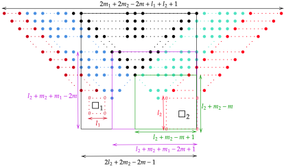
Figure 26: If the central window overshoots both $\Box_{1}$ and $\Box_{2}$, it contains $\Box$ (black). Sequences in $S_{2}$ have a window containing the green rectangle but not the purple rectangle.

As $\Box$ is a square and contains both $\Box_{1}$ and $\Box_{2}$, it has side length $L\geq l_{1}+l_{2}$. Lemma 3.4.5 then implies that

$$\#S_{3}\leq q^{2m_{1}+2m_{2}-2m+l_{1}+l_{2}+1-L}\leq q^{2m_{1}+2m_{2}-2m+1}.$$ (5.2.5)

Case 2.2.(ii): Cardinality of the Sets $S_{2}$ and $S_{1}$.

Consider the hat cone of $\Box_{2}$. Let $X$ be the set of sequences of length $2m_{2}+1+l_{2}$ that contain the central window and $\Box_{2}$ (that is, those containing the green rectangle in Figure 26). The size of $X$ is given by Lemma 5.1.2 with $d=1$:

$$\#X=\frac{q^{m_{2}-m}}{(q+1)^{2}}\left(2\cdot q^{2m+2}+2\cdot q^{2m+1}-q^{2}+1\right)\ll_{q}q^{m_{2}+m}.$$ (5.2.6)

Similarly, define $Y$ as the set of sequences with windows containing the purple rectangle in Figure 26. Lemma 5.1.2 gives the size of $Y$ as

$$\#Y=\frac{q^{m_{2}-2m+m_{1}+2}}{(q+1)^{2}}(2q^{2(2m-m_{1})}+2q^{2(2m-m_{1})}-q^{2}+1)\ll_{q}q^{m_{2}+2m-m_{1}}\leq q^{m_{2}+m}.$$ (5.2.7)

Here, $\#X-\#Y$ is the number of sequences whose number wall has a window containing the central window and $\Box_{2}$ but that does not touch $\Box_{1}$. By Lemma 3.4.6, every sequence counted in $\#X-\#Y$ can be extended in $q^{2m_{1}-2m}$ different ways. Hence,

$$\#S_{2}= (\#X-\#Y)\cdot q^{2m_{1}-2m}\ll_{q}q^{m_{2}+2m_{1}-m}$$ (5.2.8)

The proof of the inequality

$$\#S_{1}\ll_{q}q^{m_{1}+2m_{2}-m}$$ (5.2.9)

is the same, swapping the roles of $\Box_{1}$ and $\Box_{2}$.

Completion of Case 2.2.

Combining (5.2.1),(5.2.3),(5.2.9), (5.2.8) and (5.2.5) gives

$$\#S_{r,q}^{\Box_{1},\Box_{2}} =q^{2m_{1}+2m_{2}-2m+1}-q^{2m_{1}+2m_{2}-2m}+\#S_{0}+\#S_{1}+\#S_{2}+\#S_{3}$$

$$\ll_{q}q^{2m_{1}+2m_{2}-2m+1}+m\cdot q^{m_{1}+m_{2}}+q^{m_{2}+2m_{1}-m}+q^{m_{1}+2m_{2}-m}.$$ (5.2.10)

Using that $m\leq q^{m}$ for all $m,q\in\mathbb{N}$ and that $m_{i}\geq m$ gives

$$(\ref{total}) \ll_{q}q^{2m_{1}+2m_{2}-2m+1}.$$

Multiplying by the $q^{r-(2m_{1}+2m_{2}-2m+l_{1}+l_{2}+1)}$ arbitrary continuations completes the proof of Case 2.

Case 3

The third and final case is when the hat cone of one window is contained fully within the hat cone of the other. Assume without loss of generality that the hat cone of $\Box_{1}$ is contained inside the hat cone of $\Box_{2}$, and that $\Box_{1}$ appears on the right side of or above $\Box_{2}$. Extend the hat generator of $\Box_{1}$ on the right until it reaches the end of the hat generator of $\Box_{2}$. For this case, this is called the extended hat generator of $\Box_{1}$. There are two sub-cases.

Case 3.1:

Here, the number wall generated by the extended hat generator of $\Box_{1}$ has depth greater than $m_{2}$, as illustrated below:

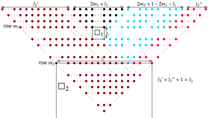
Figure 27: The hat cone of $\Box_{1}$ is in black. The blue and light red combined denote the number wall generated by the extended hat cone of $\Box_{1}$, with the blue portion showing where the number wall has depth $m_{2}$. The entire number wall is the hat cone of $\Box_{2}$.

Corollary 3.4.5 shows there are $q^{2m_{1}}$ sequences of length $2m_{1}+l_{1}$ which are hat generators for $\Box_{1}$. Using Lemma 3.4.6, there are $q^{2m_{2}-2m_{1}-l_{1}}$ continuations to the hat generator of $\Box_{1}$ on the right-hand side with length $2m_{2}+1-2m_{1}-l_{1}$ such that the lowest light blue entry in Figure 27 is zero. Lemma 3.2.4 shows there is at most a single continuation of length $l_{2}^{\prime\prime}$ on the right-hand side and of length $l_{2}^{\prime}$ on the left-hand side such that the number wall has a window containing $\Box_{2}$, although sometimes such a continuation may not exist. Hence, there are at most $q^{2m_{2}-l_{1}}$ sequences with windows containing $\Box_{1}$ and $\Box_{2}$ in their number wall. Multiplying by $q^{r-2m_{2}-l_{2}}$ for all the arbitrary choices of the sequence that are not in the hat generator of $\Box_{2}$ yields, as required,

$$\#S_{r,q}^{\Box_{1},\Box_{2}}<q^{r-l_{1}-l_{2}}.$$

Case 3.2:

Here, the number wall generated by the extended hat generator of $\Box_{1}$ has depth $m<m_{2}$. Without loss of generality, assume $\Box_{1}$ is to the right of $\Box_{2}$. Once again, there are two sub-cases:

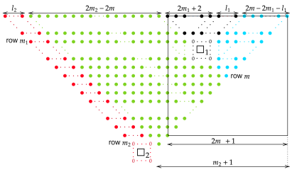
Figure 28: The number wall generated by the extended hat cone of $\Box_{1}$ is coloured in black and light blue.

• If $m_{2}>2m$, then every possible sequence of length $2m+1$ only has windows that undershoot $\Box_{2}$, as illustrated in Figure 28. Hence, for any of the arbitrary $q^{2m-2m_{1}-l_{1}}$ continuations of the hat generator of $\Box_{1}$, Lemma 3.4.6 shows there are $q^{2m_{2}-2m}$ continuations giving a window containing $\Box_{2}$. This gives a total of $q^{2m_{2}-l_{1}}$ sequences of length $2m_{2}+l_{2}$ with windows containing $\Box_{1}$ and $\Box_{2}$. Multiplying by the $q^{r-(2m_{2}-l_{2})}$ arbitrary continuations completes the proof.

• If $m_{2}\leq 2m$, the number wall generated by the extended hat generator for $\Box_{1}$ either has no window on row $m$ or else a window that undershoots, hits or overshoots $\Box_{2}$.

  • If such a window does not exist, or it undershoots $\Box_{2}$, then Corollary 3.4.4 or Lemma 3.4.6 show there are $q^{2m_{2}-2m}$ left-side extensions that give a number wall with a window containing $\Box_{2}$. Hence, as an over-estimate, there are less than or equal to $q^{2m-2m_{1}-l_{1}}$ right-side continuations of the hat generator for $\Box_{1}$ that satisfy this criteria. Therefore, these cases contribute at most $q^{2m_{2}-l_{1}}$ to the total.

  • If a window $\Box$ in the number wall overshoots $\Box_{2}$ then it also contains $\Box_{1}$. Let $l\geq l_{1}+l_{2}+1$ be the size of $\Box$. This is illustrated below:

    

    Figure 29: If a sequence has a zero portion in the shape of the minimal rectangle containing $\Box_{1}$ and $\Box_{2}$ (dashed, yellow), it necessarily contains the full square window (black).

    By Corollary 3.4.5 there are less than or equal to $q^{2m_{2}-l_{1}-1}$ sequences in this case.
    This completes the proof of Theorem 5.2.1.

∎

6 A Khintchine-Type Result in $p(t)$-adic Approximation

This section contains the proof of Theorem 1.0.6. This is a corollary of the following theorem, proved using the combinatorial statements established in the previous section.

Theorem 6.0.1.

Let $f:\{q^{k}\}_{k\geq 0}\cup\{0\}\to\mathbb{R}+$ be a increasing function and $p(t)\in\mathbb{F}_{q}[t]$ be an irreducible polynomial. For $\mu$-almost every Laurent series $\Theta\in\mathbb{I}$, the inequality

$$N(t)\cdot f(|N(t)|)\cdot|N(t)|_{p(t)}\cdot\left|\left\langle|N(t)|\cdot\Theta(t)\right\rangle\right|\leq\frac{1}{q}$$ (6.0.1)

has infinitely (finitely, respectively) many solutions if

$$\sum_{k\geq 0}\frac{k}{f\left(q^{k}\right)}$$ (6.0.2)

diverges (converges, respectively).

Theorem 6.0.1 implies Theorem 1.0.6. To show this, the following set is defined: fix a polynomial $N(t)=M(t)\cdot t^{k}$ where $k\in\mathbb{N}\cup\{0\}$ and $M(t)$ is coprime to $t$. Define $h:=\deg(M(t))$, implying $h+k=\deg(N(t))$, and let

$$A_{N(t),f}:=\left\{\Theta(t)\in\mathbb{I}:N(t)\cdot f(|N(t)|)\cdot|N(t)|_{p(t)}\cdot\left|\left\langle|N(t)|\cdot\Theta(t)\right\rangle\right|\leq q^{-1}\right\}.$$ (6.0.3)

Proof of Theorem 1.0.6 modulo Theorem 6.0.1.

If the sum 6.0.2 converges, the proof is clear. In the divergence case, the set $W(f,t)$ (defined in equation (1.0.10)) is expressed as

$$W(f,t)=\bigcap_{i=0}^{\infty}\bigcap_{N(t)\in\mathbb{F}_{q}[t]\backslash\{0\}}A_{N,q^{i}f}.$$

As this is a countable intersection of full measure sets, $W(f,t)$ has full measure. ∎

From now on, $A_{N(t),f}$ is written as $A_{N(t)}$.

Completion of the proof of Theorem 1.0.6.

The Convergent Case

Recall the notation of a ball in the field of Laurent series, introduced in (1.0.9). Given an irreducible polynomial $p(t)$, the set $A_{N(t)}$ is decomposed as follows:

$$A_{N(t)} =\bigcup_{P\in(\mathbb{F}_{q}[t])_{\deg(N)}}\left\{\Phi\in\mathbb{I}:\left|N\Phi-P\right|\leq\frac{q^{-1}}{f(|N|)\cdot|N|\cdot|N|_{p(t)}}\right\}$$

$$=\bigcup_{P\in(\mathbb{F}_{q}[t])_{\deg(N)}}B\left(PN^{-1},\frac{q^{-1}}{f(|N|)\cdot|N|^{2}\cdot|N|_{p(t)}}\right).$$ (6.0.4)

This implies that

$$\mu(A_{N(t)})\leq q^{\deg(N)+1}\frac{q^{-1}}{f(|N|)\cdot|N|^{2}\cdot|N|_{p(t)}}=\frac{1}{f(|N|)\cdot|N|\cdot|N|_{p(t)}}\cdotp$$

Define $m:=\deg(p(t))$. Rewriting $N$ as $N=M\cdot p(t)^{k}$ for $M\in\mathbb{F}_{q}[t]$ such that $(M,p(t))=1$ and for $k\in\mathbb{N}\cup\{0\}$ gives

$$\sum_{N\in\mathbb{F}_{q}[t]\backslash\{0\}}\frac{1}{f(|N|)\cdot|N|\cdot|N|_{p(t)}} =\sum_{\begin{subarray}{c}M\in\mathbb{F}_{q}[t]\backslash\{0\}\\ (M,p(t))=1\end{subarray}}\sum_{k\geq 0}\frac{1}{f(|p(t)|^{k}\cdot|M|)\cdot|M|}\cdotp$$ (6.0.5)

Define $h=\deg(M(t))$ and expand $M(t)$ as

$$M=\sum_{i=0}^{H}A_{i}(t)p(t)^{i},$$

where $A_{i}(t)\in\left(\mathbb{F}_{q}[t]\right)_{m-1}$, $H=\left\lfloor\frac{h}{m}\right\rfloor$ and $\deg(A_{H})=h-mH$. If $(M,p(t))=1$, this also implies that $A_{0}(t)\neq 0$. Assuming $h\geq m$, there are

$$\underbrace{(q^{m}-1)}_{\begin{subarray}{c}\text{coefficients of}\\ A_{0}(t)\neq 0\end{subarray}}\cdot\underbrace{q^{m(H-1)}}_{\begin{subarray}{c}\text{ coefficients of }\\ A_{1}(t),\dots,A_{H-1}(t)\end{subarray}}\cdot\underbrace{q^{h-mH-1}\cdot(q-1)}_{\begin{subarray}{c}\text{ coefficients of}\\ A_{H}(t)\end{subarray}}\asymp q^{h}$$

such polynomials $M$. If $h\leq m$, then any of the $q^{h+1}-1$ nonzero polynomials of degree $h$ are coprime to $p(t)$. Hence,

$$(\ref{pt borel})=\sum_{h\geq 0}\sum_{\begin{subarray}{c}M\in\mathbb{F}_{q}[t]\backslash\{0\}\\ (M,p(t))=1\\ \deg(M)=h\end{subarray}}\sum_{k\geq 0}\frac{1}{f(|p(t)|^{k}\cdot|M|)\cdot|M|}\asymp\sum_{h\geq 0}\sum_{k\geq 0}\frac{1}{f(q^{h+mk})}\cdotp$$ (6.0.6)

Defining the exponent $i:=h+mk$, and since $h\equiv i\mod m$, each value of $i$ appears in (6.0.6) $\left\lfloor\frac{i}{m}\right\rfloor=H+k$ times. Thus,

$$(\ref{pt borel2})\ll\sum_{i\geq 0}\frac{i}{m\cdot f(q^{i})}\cdot\ll\sum_{i\geq 0}\frac{i}{f(q^{i})}\cdotp$$

Applying the Borel-Cantelli lemma proves the convergence case.

The Divergence case:

The problem is rephrased in terms of number walls. If $\Theta(t)\in A_{N(t)}$, Theorem 1.0.5 implies there is a window of size $\left\lfloor\log_{q}(f(q^{h+k}))\right\rfloor$ in column $h+k+1$ and row $h$ of the number wall generated by $\Theta(t)$. This is the window represented by $\mathbf{N(t)}$, denoted $\Box_{N(t)}$. By Corollary 3.4.5, for $r$ a large natural number, there are $q^{r-\left\lfloor\log_{q}(f(q^{h+k}))\right\rfloor}$ possible sequences of length $r$ over $\mathbb{F}_{q}$ whose number wall contains $\Box_{N(t)}$. However, it is clear that $\Box_{N(t)}$ only depends on $k$ and $h$, and not the specific choice of $M(t)$. This motivates the following definition: for $h,k\in\mathbb{N}$, define the set

$$A_{h,k}:=\left\{\Theta(t)\in A_{N(t)}:N(t)=M(t)\cdot t^{k},\leavevmode\nobreak\ \deg(M(t))=h,\leavevmode\nobreak\ (M(t),t)=1\right\}.$$

Explicitly, $A_{h,k}$ is the union of all the sets $A_{N(t)}$ which can expressed as $N(t)=M(t)\cdot t^{k}$ for some polynomial $M(t)$ of degree $h$. In particular, $A_{h,k}$ is the union of finitely many sets $A_{N(t)}$. Therefore, if $\Theta(t)$ is in the set $A_{N(t)}$ for infinitely many $N(t)\in\mathbb{F}_{q}[t]$ then $\Theta(t)$ is also in infinitely many sets $A_{h,k}$. The converse is also clear, implying

$$\limsup_{|N(t)|\to\infty}A_{N(t)}=\limsup_{\min(h,k)\to\infty}A_{h,k}.$$

Similarly as above, define $\Box_{h,k}$ as the window represented by any $N(t)$ which can be decomposed as $M(t)\cdot t^{k}$, where $\deg(M(t))=h$ and $M(t)$ and $t$ are coprime.

The following classical lemma is used to attain positive measure of $W(f,t)$ from the divergence of the series (6.0.2). The reader is referred to [11] for the proof and further reading.

Lemma 6.0.2 (Divergence Borel-Cantelli).

Let $\{E_{n}\}_{n\in\mathbb{N}}$ be a sequence measureable sets in a space with measure $\mu$. Define $E_{\infty}:=\limsup_{n\to\infty}E_{n}$. Assume $\sum_{n\geq 0}\mu(E_{n})=\infty$ and that there exists a constant $C>0$ such that the inquality

$$\sum_{s,t\leq r}\mu(E_{s}\cap E_{t})\leq C\left(\sum_{n\leq r}\mu(E_{n})\right)^{2}$$

holds for infinitely many $r\in\mathbb{N}$. Then $\mu(E_{\infty})\geq 1/C$.

This lemma is now used to show that $A_{\infty}=\limsup_{\min(h,k)\to\infty}A_{h,k}$ has positive measure when $p(t)=t$. The case of any irreducible polynomial will be inferred from this one afterwards.

Let $N(t)\in\mathbb{F}_{q}[t]$ be a polynomial. The sum

$$\sum_{h_{1}\leq r}\sum_{k_{1}\leq r-h_{1}}\sum_{h_{2}\leq r}\sum_{k_{2}\leq r-h_{2}}\mu(A_{h_{1},k_{1}}\cap A_{h_{2},k_{2}})$$

is partitioned into two pieces:

$$S_{1} =\sum_{h_{1}\leq r}\sum_{k_{1}\leq r-h_{1}}\sum_{h_{2}\leq r}\sum_{\begin{subarray}{c}k_{2}\leq r-h_{2}\\ \Box_{h_{1},k_{1}}\text{ touches }\Box_{h_{2},k_{2}}\end{subarray}}\mu(A_{h_{1},k_{1}}\cap A_{h_{2},k_{2}}),$$

and

$$S_{2} =\sum_{h_{1}\leq r}\sum_{k_{1}\leq r-h_{1}}\sum_{h_{2}\leq r}\sum_{\begin{subarray}{c}k_{2}\leq r-h_{2}\\ \Box_{h_{1},k_{1}}\text{ does not touch }\Box_{h_{2},k_{2}}\end{subarray}}\mu(A_{h_{1},k_{1}}\cap A_{h_{2},k_{2}}).$$ (6.0.7)

The sum $S_{1}$ is dealt with first. The goal is to show that

$$S_{1}\ll\left(\sum_{h\leq r}\sum_{k\leq r-h}\mu(A_{h,k})\right)^{2}=\sum_{h_{1}\leq r}\sum_{k_{1}\leq r-h_{1}}\left(\sum_{h_{2}\leq r}\sum_{k_{2}\leq r-h_{2}}\mu(A_{h_{2},k_{2}})\right)\mu(A_{h_{1},k_{1}}).$$

To achieve this, fix $h_{1}$ and $k_{1}$, then consider all the values of $h_{2}$ and $k_{2}$ such that $\Box_{h_{1},k_{1}}$ touches $\Box_{h_{2},k_{2}}$. As the size of $\Box_{h,k}$ is determined only by $h,k$ and the function $f$, there are only a finite number of windows $\Box_{h_{2},k_{2}}$ touching $\Box_{h_{1},k_{1}}$. These values are partitioned into disjoint sets $\{P_{i}\}_{i\geq 0}$ depending on how much larger than $\Box_{h_{1},k_{1}}$ a window must be to contain $\Box_{h_{1},k_{1}}$ and $\Box_{h_{2},k_{2}}$. Explicitly, $P_{i}$ contains all the pairs $(h_{2},k_{2})$ such that the minimum size of any window containing $\Box_{h_{1},k_{1}}$ and $\Box_{h_{2},k_{2}}$ is $i$ more than $\Box_{h_{1},k_{1}}$. For example, $P_{0}$ contains only the pairs $(h_{2},k_{2})$ such that $\Box_{h_{2},k_{2}}=\Box_{h_{1},k_{1}}$ (that is, $h_{2}=h_{1}$ and $k_{2}=k_{1}$). Similarly, $P_{1}$ contains all the pairs $(h_{1},k_{1})$ such that the window containing $\Box_{h_{1},k_{1}}$ and $\Box_{h_{2},k_{2}}$ is only one larger than the size of $\Box_{h_{1},k_{1}}$. Below, the diagram used in the calculation of the measure of $P_{1}$:

Figure 30: The purple square represents $\Box_{h_{1},k_{1}}$ and the coloured dots represent the pairs $(h,k)\in P_{1}$.

A window with top left corner in the red positions would have exactly the same size as $\Box_{h_{1},k_{1}}$. Then, a window in the blue (green, respectively) positions would have a size less than or equal to (greater than or equal to, respectively) the size of $\Box_{h_{1},k_{1}}$. Each starting position determines the shape of the portion of the number wall that must be full of zeros. For example, if $h_{2}$ and $k_{2}$ are such that $\Box_{h_{2},k_{2}}$ starts in the top left blue position in Figure 30, then $\Box_{h_{2},k_{2}}$ has size less than or equal to $\Box_{h_{1},k_{1}}$ and hence $\Box_{h_{1},k_{1}}$ and $\Box_{h_{2},k_{2}}$ are contained in a single square of length $l_{1}+1$. Let $\Box$ be a window of size $l$. Using Corollary 3.4.5 and the ultrametic property of the absolute value gives

$$\mu(\{\Theta\in\mathbb{F}_{q}((t^{-1})):\Theta\text{ contains }\Box\text{ in its number wall}\})=q^{r-l}\cdot q^{r}=q^{-l}.$$

Hence, in this case

$$\mu(A_{h_{1},k_{1}}\cap A_{h_{2},k_{2}})=q^{-l_{1}-1}.$$

Similarly, if $h_{2}$ and $k_{2}$ are such that $\Box_{h_{2},k_{2}}$ starts in the top middle blue position, then $\Box_{h_{1},k_{1}}$ and $\Box_{h_{2},k_{2}}$ are contained inside a rectangle with height one greater than its width. In this case, Lemma 5.1.2 implies that

$$\mu(A_{h_{1},k_{1}}\cap A_{h_{1}-1,k_{1}})\ll 2q^{-l_{1}-1}.$$

Doing a similar calculation for the other six pairs $(h_{2},k_{2})\in P_{1}$ shows that

$$\sum_{(h_{2},k_{2})\in P_{1}}\mu(A_{h_{1},k_{1}}\cap A_{h_{2},k_{2}})\leq 8\cdot\mu(A_{h_{1},k_{1}}\cap A_{h_{1}-1,k_{1}})\ll\cdot q^{-l_{1}-1}.$$

Similarly, the following diagram depicts starting positions for $\Box_{h_{2},k_{2}}$ when $(h_{2},k_{2})\in P_{i}$.

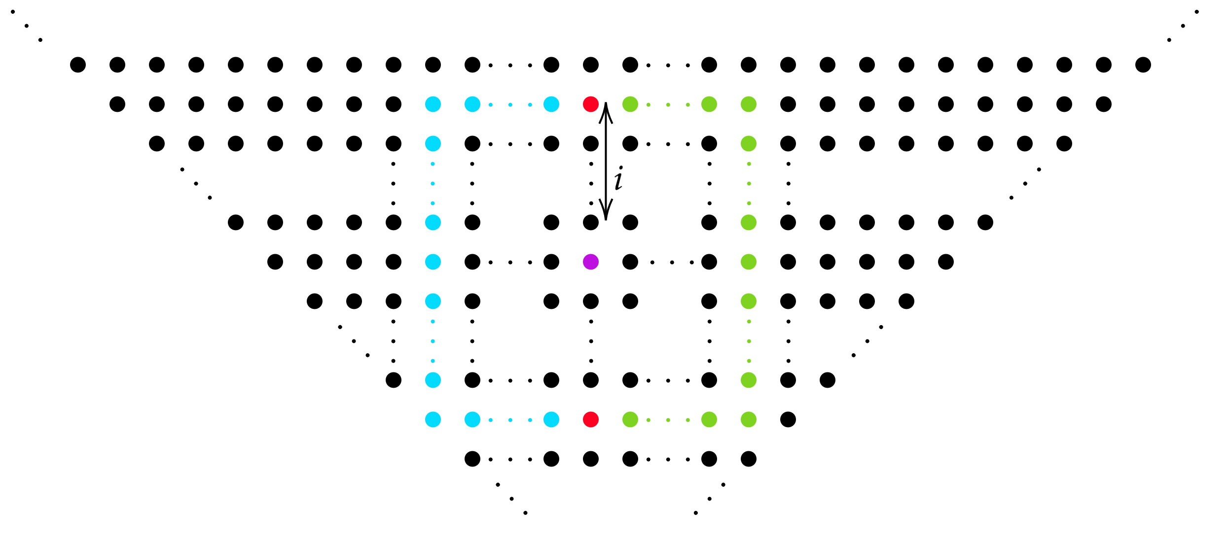
Figure 31: The coloured dots represent the pairs in $P_{i}$.

There are $8i$ pairs $(h_{2},k_{2})\in P_{i}$. If $h_{2}$ and $k_{2}$ are such that $\Box_{h_{2},k_{2}}$ starts on the top middle blue position, then $\Box_{h_{1},k_{1}}$ and $\Box_{h_{2},k_{2}}$ are contained in a rectangle with height $i$ more than its width. Every other pair $(h-2,k-2)\in P_{2}$ has $\Box_{h_{1},k_{1}}$ and $\Box_{h_{2},k_{2}}$ contained in a rectangle with difference between width and height at most $i$. Once again, Lemma 5.1.2 implies that

$$\sum_{(h_{2},k_{2})\in P_{2}}\mu(A_{h_{1},k_{1}}\cap A_{h_{2},k_{2}})\leq 8i\cdot\mu(A_{h_{1},k_{1}}\cap A_{h_{1}-2,k_{1}})\ll 16\cdot(i+1)\cdot q^{-l_{1}-i}.$$

Depending on the function $f$, the size of the window $\Box_{h_{2},k_{2}}$ could be different from $\Box_{h_{1},k_{1}}$. This leads to some pairs $(h_{2},k_{2})\in P_{i}$ being replaced with $(h_{2}^{\prime},k_{2}^{\prime})$ representing the starting positions being moved up and to the left. In some cases, pairs in $P_{i}$ are ignored entirely. Moving a starting position does not effect the calculation and it suffices to assume none are ignored when calculating an upper bound. Furthermore, when $i=l_{1}+1,$ the sets $P_{i}$ become empty, as the windows $\Box_{h_{1},k_{1}}$ and $\Box_{h_{2},k_{2}}$ are no longer touching. Hence,

$$\sum_{h_{2}\leq r}\sum_{\begin{subarray}{c}k_{2}\leq r-h_{2}\\ \Box_{h_{1},k_{1}}\text{ touches }\Box_{h_{2},k_{2}}\end{subarray}}\mu(A_{h_{1},k_{1}}\cap A_{h_{2},k_{2}}) \ll_{q}q^{-l_{1}}\cdot\left(1+8\cdot\sum_{i=1}^{\infty}i^{2}q^{-i}\right)$$

$$=\mu(A_{h_{1},k_{1}})\cdot\left(1+8\cdot\sum_{i=1}^{\infty}i^{2}q^{-i}\right).$$ (6.0.8)

Therefore, using the assumption that

$$\sum_{h\geq 0}\sum_{k\geq 0}\mu(A_{h,k})=\infty,$$

there exists some value $r$ such that $\sum_{h+k\leq r}\mu(A_{h,k})>1$ in such a way that

$$S_{1}\leavevmode\nobreak\ \leavevmode\nobreak\ \ll\leavevmode\nobreak\ \leavevmode\nobreak\ \sum_{h+k\leq r}\mu(A_{h,k})\leavevmode\nobreak\ \leavevmode\nobreak\ <\leavevmode\nobreak\ \leavevmode\nobreak\ \left(\sum_{h+k\leq r}\mu(A_{h,k})\right)^{2}.$$

Next, $S_{2}$, as defined in (6.0.7), is dealt with. If $\Box_{h_{1},k_{1}}$ does not touch $\Box_{h_{2},k_{2}}$, then $\mu(A_{h_{1},k_{1}}\cap A_{h_{2},k_{2}}$ is given by the number of sequences that have windows containing $\Box_{h_{1},k_{1}}$ and $\Box_{h_{2},k_{2}}$ multiplied by the measure of the ball centered around them. By Theorem 5.2.1, this is

$$\mu(A_{h_{1},k_{1}}\cap A_{h_{2},k_{2}})\ll q^{r-l_{1}-l_{2}}\cdot q^{-r}=q^{-l_{1}-l_{2}}.$$

Hence,

$$S_{2} \ll\sum_{h_{1}+k_{1}\leq r}\sum_{\begin{subarray}{c}h_{2}+k_{2}\leq r\\ \Box_{h_{1},k_{1}}\text{ does not touch }\Box_{h_{2},k_{2}}\end{subarray}}q^{-\left\lfloor\log_{q}(f(q^{h_{1}+k_{1}})\right\rfloor-\left\lfloor\log_{q}(f(q^{h_{2}+k_{2}})\right\rfloor}.$$ (6.0.9)

To acquire an upper bound on this sum, the condition that $\Box_{h_{1},k_{1}}$ and $\Box_{h_{2},k_{2}}$ do not touch can be dropped:

$$(\ref{divinq1}) \leq\sum_{h_{1}+k_{1}\leq r}\sum_{h_{2}+k_{2}\leq r}q^{-\left\lfloor\log_{q}(f(q^{h_{1}+k_{1}})\right\rfloor-\left\lfloor\log_{q}(f(q^{h_{2}+k_{2}})\right\rfloor}$$

$$=\left(\sum_{h_{1}+k_{1}\leq r}q^{-\left\lfloor\log_{q}(f(q^{h_{1}+k_{1}})\right\rfloor}\right)\cdot\left(\sum_{h_{2}+k_{2}\leq r}q^{\left\lfloor\log_{q}(f(q^{h_{2}+k_{2}})\right\rfloor}\right)$$

$$=\left(\sum_{h+k\leq r}\mu(A_{h,k})\right)^{2}.$$

Hence, by the Divergence Borel-Cantelli lemma (Lemma 6.0.2), the set $A_{\infty}$ has positive measure. The following theorem is used to go from positive measure to full measure:

Proposition 6.0.3 (Zero-One Law).

Let $\phi:\mathbb{F}_{q}[t]\to\mathbb{R}$ be a function and let

$$E_{N}=\left\{\Theta\in\mathbb{I}:\left|\Theta-\frac{P}{N}\right|\leq\frac{\phi(N)}{|N|}\text{ for some polynomial }P\text{ with }\deg(P)\leq\deg(N)\text{ and }(P,N)=1\right\}.$$

Then $\mu(\limsup_{|N|\to\infty}E_{N})\in\{0,1\}$.

The proof of this proposition is completed by Inoue and Nakada in [12, Theorem 4]. It is a direct adaptation of the proof in the real case, provided by Gallagher in [10]. The sets $E_{N}$ in the statement of Proposition 6.0.3 are the sets $A_{N(t)}$ from (6.0.3), and hence positive measure of $A_{h,k}$ implies full measure. The proof in the case $p(t)=t$ is thus complete.

Finally, the $p(t)=t$ case is shown to imply the divergence part of the theorem for an arbitrary irreducible polynomial $p(t)$. Assume that the sum (1.0.12) diverges and let $N(t)\in\mathbb{F}_{q}[t]$ and $\Theta(t)\in\mathbb{F}_{q}((t^{-1}))$ be a pair satisfying the inequality (6.0.1). If $b,c\in\mathbb{Z}$ and $\Xi(t)=\sum_{i=b}^{c}a_{i}t^{i}\in\mathbb{F}_{q}((t^{-1}))$, then $\Xi(p(t)):=\sum_{i=b}^{c}a_{i}p(t)^{i}$. If $m=\deg(p(t))$ and $k$ and $l$ are natural numbers such that

$$|N(t)|_{t}:=q^{-k} \left|\left\langle N(t)\cdot\Theta(t)\right\rangle\right|=q^{-l},$$ and

then

$$|N(p(t))|_{p(t)}=q^{-mk} \left|\left\langle N(p(t)\cdot\Theta(p(t))\right\rangle\right|=q^{-lm}.$$ and

Hence,

$$|N(p(t))|_{p(t)}\cdot |N(p(t))|\cdot f(|N(t)|)^{m}\cdot\left|\left\langle N(p(t))\cdot\Theta(p(t))\right\rangle\right|$$

$$= \left(|N(t)|\cdot f(|N(t)|)\cdot|N(t)|_{t}\cdot\left|\left\langle N(t)\cdot\Theta(t)\right\rangle\right|\right)^{m}\leq q^{-m}.$$ (6.0.10)

The following lemma is used to extend the $p(t)=t$ case to a general irreducible polynomial $p(t)$:

Lemma 6.0.4.

Define $f^{\prime}(q^{k}):=f(q^{km})^{\frac{1}{m}}$. If $\sum_{k\geq 1}\frac{k}{f(q^{k})}=\infty,$ then $\sum_{k\geq 1}\frac{k}{f^{\prime}(q^{k})}=\infty.$

For now, take Lemma 6.0.4 for granted. Note that $f^{\prime}(|N(t)|)^{m}=f(|N(p(t))|)$. The $p(t)=t$ case of Theorem 6.0.1 and the equation (6.0.10) show that for $\mu$-almost all $\Theta(t)\in\mathbb{I}$,

$$|N(p(t))|_{p(t)}\cdot|N(p(t))|\cdot f(|N(p(t))|)\cdot\left|\left\langle N(p(t))\cdot\Theta(p(t))\right\rangle\right|\leq q^{-m}.$$ (6.0.11)

Define the set

$$\vartheta:=\{\Theta(p(t))\in\mathbb{F}_{q}((p(t)^{-1})):\Theta(p(t))\text{ satisfies (\ref{infmany}) for infinitely many }N(p(t))\in\mathbb{F}_{q}[p(t)]\},$$

and let $t^{i}\vartheta=\{t^{i}\cdot\Theta(p(t)):\Theta(p(t)\in\vartheta\}$. If $j$ is the highest power of $t$ in any Laurent series in $t^{i}\vartheta$, then it is clear that $j\equiv i\mod m$. Therefore, every Laurent series $\Xi(t)$ in the Minkowski sum

$$M(\vartheta):=\bigoplus_{i=0}^{m-1}t^{i}\vartheta$$

satisfies

$$|N(p(t))|_{p(t)}\cdot|N(p(t))|\cdot f(|N(p(t))|)\cdot\left|\left\langle N(p(t))\cdot\Xi(p(t))\right\rangle\right|\leq q^{-1}.$$

To see that $M(\vartheta)$ has full measure, let $B$ be an arbitrary ball in $\mathbb{F}_{q}((t^{-1}))$ and

$$B_{p(t)}=\{\Theta(p(t)):\Theta(t)\in B\}.$$

It is clear that $B=M(B_{p(t)})$. As the Haar measure of a set is defined as the infimum over all coverings of that set with balls, this is sufficient to conclude $\mu(M(\vartheta))=1$. This implies $M(\vartheta)$ has full measure. It remains to proof Lemma 6.0.4:

Proof of Lemma 6.0.4.

If $m=1$, then the claim is trivial. Therefore, assume $m\geq 2$. Since the series (1.0.12) diverges, for any $c,\varepsilon>0$ there exist infinitely many $k\in\mathbb{N}$ such that

$$f(q^{k})<\frac{k^{2+\varepsilon}}{c}.$$ (6.0.12)

Let $I\subset\mathbb{N}$ be the set of all natural numbers $k$ satisfying (6.0.12). Furthermore, define

$$J=\left\{k\in I:f(q^{k})<k^{1+\varepsilon}\right\}.$$

Then, at least one of the following is true:

$$\sum_{k\in J}\frac{k}{f(q^{k})}=\infty \sum_{k\in I\backslash J}\frac{k}{f(q^{k})}=\infty.$$ or (6.0.13)

This follows from the definition of the set $\mathbb{I}$ and from the identity

$$(\ref{metsum2})=\sum_{k\in J}\frac{k}{f(q^{k})}+\sum_{k\in I\backslash J}\frac{k}{f(q^{k})}+\underbrace{\sum_{k\not\in I}\frac{k}{f(q^{k})}}_{<\infty}=\infty.$$

Assume the first case of (6.0.13) holds. Then, $J$ is clearly infinite and

$$\sum_{k\in J}\frac{k}{f^{\prime}(q^{k})} =\sum_{k\in J}\frac{k}{f(q^{km})^{\frac{1}{m}}}\leavevmode\nobreak\ \gg_{m,\varepsilon}\leavevmode\nobreak\ \sum_{k\in J}k^{1-\frac{1+\varepsilon}{m}}=\infty.$$ (6.0.14)

Now, assuming the second case of (6.0.13),

$$\sum_{k\in I\backslash J}\frac{k}{f^{\prime}(q^{k})} =\sum_{k\in I\backslash J}\frac{k}{f(q^{km})^{\frac{1}{m}}}\gg_{m,\varepsilon}\sum_{k\in I\backslash J}k^{1-\frac{2+\varepsilon}{m}}.$$ (6.0.15)

If $m>2$ and $\varepsilon$ is sufficiently small, (6.0.15) trivially diverges. If $m=2$, from the definition of $k\in I\backslash J$:

$$(\ref{I}) =\sum_{k\in I\backslash J}k^{\frac{-\varepsilon}{2}}\geq\sum_{k\in I\backslash J}\frac{k}{f(q^{k})}=\infty.$$ (6.0.16)

Therefore, both cases of (6.0.13) have a divergent subsequence and the proof is complete. ∎

This completes the proof of Theorem 6.0.1. ∎

7 Open Problems

Theorem 1.0.3 has reduced disproving $p(t)$-LC to disproving $t$-LC. OVer the duration of this work, python code [16] was written that generated the number walls of any given finite sequence. This provides strong experimental evidence that the counterexample to $t$-LC over $\mathbb{F}_{3}$ from [1] is also a counterexample to $t$-LC over $\mathbb{F}_{p}$ for $p$ congruent to 3 modulo 4. Furthermore, define the Adapted Paper-Folding Sequence as $(f_{n})_{n\in\mathbb{N}}$ as

$$f_{n}=\frac{k_{n}-1}{2},$$

where $k_{n}$ is the greatest odd factor of $n$ reduced modulo 8. There is equally strong experimental evidence that this is a counterexample to $t$-LC over fields of characteristic $p$ congruent to $1$ modulo 4. The code [16] has also been used to show that every sequence over $\mathbb{F}_{2}$ has windows of size at least 3 in its number wall. There is no obvious reason this should not be true when $3$ is replaced by any natural number. This leads to the following conjecture.

Conjecture 7.0.1.

The $t$-adic Littlewood Conjecture is true over $\mathbb{F}_{2}$, but false over all other finite fields.

A second natural continuation is to try and improve Theorem 1.0.7. However, doing so would require a new method. An obvious suggestion would be to adapt the method of Badziahin and Velani from [17] to get full dimension with a growth function of $\log(|N|)\cdot\log(\log(|N|))$, as they do in the real case. However, any attempt to do this has been unsuccessful. A finite number wall generated by a sequence of length $n$ has $O(n^{2})$ points. This is the reason for the $\log^{2}$ term in Theorem 1.0.7 and it motivates the following conjecture:

Conjecture 7.0.2.

The set of counterexamples to $t$-LC with growth function $f$ has zero Hausdorff dimension when $f$ is of the form $\log^{1+\lambda}$ for any $\lambda<1$.

This is a departure from the real case, where it is conjectured the equivalent set has full Hausdorff dimension for $f=\log$.

References

- [1] Faustin Adiceam, Erez Nesharim and Fred Lunnon “On the t-adic Littlewood Conjecture” In Duke Mathematical Journal 170(10) United States: Duke University Press, 2021, pp. 2371–2419
- [2] Yann Bugeaud, Alan Haynes and Sanju Velani “Metric Considerations Concerning The Mixed Littlewood Conjecture” In International Journal of Number Theory 07.03, 2011, pp. 593–609 DOI: 10.1142/S1793042111004289
- [3] Yann Bugeaud and Bernard Mathan “On a mixed Littlewood conjecture in fields of power series” In AIP Conference Proceedings 976, 2008, pp. 19–30 DOI: 10.1063/1.2841906
- [4] Yann Bugeaud and Nikolay Moshchevitin “Badly approximable numbers and Littlewood-type problems” In Mathematical Proceedings of the Cambridge Philosophical Society 150.2 Cambridge University Press, 2011, pp. 215–226 DOI: 10.1017/S0305004110000605
- [5] John H. Conway and Richard K. Guy “The Book of Numbers” Copernicus New York, NY, 1995, pp. 310 DOI: https://doi.org/10.1007/978-1-4612-4072-3
- [6] Manfred Einsiedler, Anatole Katok and Elon Lindenstrauss “Invariant Measures and the Set of Exceptions to Littlewood’s Conjecture” In Annals of Mathematics 164.2 Annals of Mathematics, 2006, pp. 513–560 URL: http://www.jstor.org/stable/20159999
- [7] Manfred Einsiedler and Dmitry Kleinbock “Measure rigidity and -adic Littlewood-type problems” In Compositio Mathematica 143.3 London Mathematical Society, 2007, pp. 689–702 DOI: 10.1112/S0010437X07002801
- [8] Manfred Einsiedler, Elon Lindenstrauss and Amir Mohammadi “Diagonal actions in positive characteristic” In Duke Mathematical Journal 169, 2017, pp. 117\bibrangessep175 DOI: 10.1215/00127094-2019-0038
- [9] Kenneth J. Falconer “Techniques for Calculating Dimensions” In Fractal Geometry: Mathematical Foundations and Applications John Wiley & Sons, Ltd, 2003, pp. 59–75 DOI: https://doi.org/10.1002/0470013850.ch4
- [10] Patrick Gallagher “Approximation by reduced fractions” In Journal of the Mathematical Society of Japan 13.4 The Mathematical Society of Japan, 1961, pp. 342–345
- [11] G. Harman and S.M.G. Harman “Metric Number Theory”, London Mathematical Society monographs Clarendon Press, 1998
- [12] Kae Inoue and Hitoshi Nakada “On metric Diophantine approximation in positive characteristic” In Acta Arithmetica 110, 2003, pp. 205–218 DOI: 10.4064/aa110-3-1
- [13] Fred Lunnon “The Pagoda Sequence: a Ramble through Linear Complexity, Number Walls, D0L Sequences, Finite State Automata, and Aperiodic Tilings” In Electronic Proceedings in Theoretical Computer Science 1 Open Publishing Association, 2009, pp. 130–148 DOI: 10.4204/eptcs.1.13
- [14] William Lunnon “The number-wall algorithm: An LFSR cookbook” In Journal of Integer Sequences 4, 2001, pp. 2–3
- [15] Bernard Mathan and Olivier Teulié “Problèmes diophantiens simultanés” In Monatshefte für Mathematik 143, 2004, pp. 229–245 DOI: 10.1007/s00605-003-0199-y
- [16] Steven Robertson “Number Wall Code” URL: https://github.com/Steven-Robertson2229/Number-Wall-Code.git
- [17] Sanju Velani and Dzmitry Badziahin “Multiplicatively badly approximable numbers and generalised Cantor sets” In Advances in Mathematics 228.5 Academic Press Inc., 2011, pp. 2766–2796 DOI: 10.1016/j.aim.2011.06.041
- [18] George Weiss “The Theory of Matrices. vol. 1 and vol. 2. F. R. Gantmacher.” In Science 131.3408 Chelsea Publishing Company, 1960, pp. 1216–1216 DOI: 10.1126/science.131.3408.1216.b