A hybrid finite element/neural network solver and its application to the Poisson problem

Abstract

We analyze a hybrid method that enriches coarse grid finite element solutions with fine scale fluctuations obtained from a neural network. The idea stems from the Deep Neural Network Multigrid Solver (DNN-MG)  [1] which embeds a neural network into a multigrid hierarchy by solving coarse grid levels directly and predicting the corrections on fine grid levels locally (e.g. on small patches that consist of several cells) by a neural network. Such local designs are quite appealing, as they allow a very good generalizability. In this work, we formalize the method and describe main components of the a-priori error analysis. Moreover, we numerically investigate how the size of training set affects the solution quality.

1 Introduction

Recent advancements in employing neural networks to approximate solutions to partial differential equations (PDEs) mostly focus on Physics Inspired Neural Networks (PINNs) [2] such as the Deep Ritz method [3]. They leverage the expressive power of neural networks while incorporating physical principles and promise substantial efficiency increase for high dimensional or parameter dependent partial differential equations. One main drawback of PINNs is that they need to re-train when the problem parameters change. Also, for classical problems, such as three dimensional fluid dynamics problems, highly sophisticated and well established discretization methods regarding the efficiency and accuracy are available that beat neural network approaches by far.

The method of this paper was introduced as main component the of DNN-MG [1] for the instationary Navier-Stokes equations. At each time step, a coarse solution is obtained by a classical finite element solver and corrections to finer grids are predicted locally via neural networks. Here, we focus on a simpler linear problem and aim to understand the mechanism of such a hybrid approaches by discussing its a-priori errors and via numerical experiments.

Let $\Omega\subset\mathbb{R}^{d},\;d\in\{2,3\}$ be a domain with polygonal boundary. We are interested in the weak solution of the Poisson’s equation

$$-\Delta u=f,\quad u|_{\partial\Omega}=0,$$ (1)

with a given force term $f\in H^{-1}(\Omega)$.

For a subdomain $\omega\subseteq\Omega$, let $\mathcal{T}_{h}(\omega)=\{T_{i}\}_{i=1}^{M}$ be a non-overlapping admissible decomposition of $\omega$ into convex polyhedral elements $T_{i}$ such that $\overline{\omega}=\cup_{i=1}^{M}\overline{T}_{i}$. The diameter of element $T$ is denoted by $h_{T}$ and $h=\max_{T\in\mathcal{T}_{h}(\Omega)}h_{T}$. With $\|\cdot\|_{2}$ we denote the Euclidean norm and for $v\in C(\overline{\omega})$ we define

$$\|v\|_{l^{2}(\omega)}:=\Big{(}\sum\limits_{x\text{ is node of }\mathcal{T}_{h}(\omega)}v(x)\Big{)}^{\frac{1}{2}}.$$

Moreover, let $V_{h}^{(r)}$ be the space of piecewise polynomials of degree $r\geq 1$ satisfying the homogeneous Dirichlet condition on the boundary $\partial\Omega$, i.e.

$$V_{h}:=\left\{\phi\in C(\overline{\Omega})\text{ s.t. }\;\phi|_{T}\in P^{(r)}(T)\;\forall T\in\Omega_{h},\;\phi|_{\partial\Omega}=0\right\},$$

where $P^{(r)}(T)$ is the space of polynomials of degree $r$ on a cell $T\in\mathcal{T}_{h}$. We assume that there is a hierarchy of meshes

$$\mathcal{T}_{H}(\Omega):=\mathcal{T}_{0}\preccurlyeq\mathcal{T}_{1}\preccurlyeq\cdots\preccurlyeq\mathcal{T}_{L}=:\mathcal{T}_{h}(\Omega),$$

where we denote by $\mathcal{T}_{l-1}\preccurlyeq\mathcal{T}_{l}$, that each element of the fine mesh $T\in\mathcal{T}_{l}$ originates from the uniform refinement of a coarse element $T^{\prime}\in\mathcal{T}_{l-1}$, for instance, uniform splitting of a quadrilateral or triangular element into four and of a hexahedral or tetrahedral element into eight smaller ones, respectively. Accordingly we have the nesting $V_{h}^{(l-1)}\subset V_{h}^{(l)},\quad l=1,\dots,L$ where $V_{h}^{(l)}$ is the space defined on the mesh level $l$. With a patch $\mathcal{P}\in\mathcal{T}_{h}(\Omega)$ we refer to a polyhedral subdomain of $\Omega$, but for simplicity we assume that each patch corresponds to a cell of $\mathcal{T}_{H}(\Omega)$. By $V_{h}(\mathcal{P})$ we denote the local finite element subspace

$$V_{h}(\mathcal{P}):=\operatorname{span}\left\{\phi_{h}|_{\mathcal{P}},\;\phi_{h}\in V_{h}\right\}$$

and $R_{\mathcal{P}}:V_{h}\to V_{\mathcal{P}}$ denotes the restriction to the local patch space, defined via

$$R_{\mathcal{P}}(u_{h})(x_{i})=u_{h}(x_{i})\quad\text{for each node }x_{i}\in\mathcal{T}_{h}(\mathcal{P}).$$

The prolongation $P_{\mathcal{P}}:V_{h}(\mathcal{P})\to V_{h}$ is defined by

$$P_{\mathcal{P}}(v)(x)=\begin{cases}\frac{1}{n}v(x)&x\text{ is a node of }\mathcal{T}_{h}(\mathcal{P}),\qquad n\in\mathbb{N}\text{ being the number of patches containing the node $x$}\\ 0&\text{otherwise}.\end{cases}$$ (2)

The classical continuous Galerkin finite element solution of the problem (1) is $u_{h}\in V_{h}$ s.t.

$$(\nabla u_{h},\nabla\phi)=(f,\phi)\quad\forall\phi\in V_{h},$$ (3)

with the $L^{2}$ inner product $(\cdot,\cdot)$. We are interested in the scenario where one prefers not to solve (3) on the finest level $V_{h}$ due to lacking hardware resources or too long computational times, but in $V_{H}$ with $H\gg h$. This is the so-called coarse solution $u_{H}\in V_{H}$ and fulfills $(\nabla u_{H},\nabla\phi)=(f,\phi)\quad\forall\phi\in V_{H}$. The key idea of our method is to obtain the fine mesh fluctuations $u_{h}-u_{H}$ in forms of neural network updates $w_{\mathcal{N}}$ corresponding to the inputs $u_{H}$ and $f$. Hence, the neural network updated solution has the form $u_{\mathcal{N}}:=u_{H}+w_{\mathcal{N}}$ in the case where the network operates globally on the whole domain. A more appealing setting is where these updates are obtained locally, such that the network is acting on the data not on the whole domain at once, but on small patches $\mathcal{P}\in\mathcal{T}_{h}(\Omega)$. In this case, while the training is performed in a global manner, the updates are patch-wise and the network updated solution has the form $u_{\mathcal{N}}:=u_{H}+\sum_{\mathcal{P}}P_{\mathcal{P}}w^{\mathcal{P}}_{\mathcal{N}}$.

2 Hybrid finite element neural network discretization

2.1 Neural network

In this section we introduce the neural network we use and formalize the definition of finite element/neural network solution.

Definition 1 (Multilayer perceptron).

Let $L\in\mathbb{N}$ be the number of layers and let $N_{i}$ be the number of neurons on layer $i\in\{1,\dots,L\}$. Each layer $i\in\{1,\dots,{L-1}\}$ is associated with a nonlinear function $l_{i}(x):\mathbb{R}^{N_{i-1}}\rightarrow\mathbb{R}^{N_{i}}$ with

$$l_{i}(x)=\sigma(W_{i}x+b_{i})$$ (4)

and an activation function $\sigma:\mathbb{R}\to\mathbb{R}$. The multilayer perceptron (MLP) ${\cal N}:\mathbb{R}^{N_{0}}\to\mathbb{R}^{N_{L}}$ is defined via

$$\mathcal{N}=W_{n}(l_{n-1}\circ\dots\circ l_{1})(x)+b_{n}$$

where $W_{i}\in\mathbb{R}^{N_{i-1}\times N_{i}}$ denote the weights, and $b_{i}\in\mathbb{R}^{N_{i}}$ the biases.

2.2 Hybrid solution

On a patch $\mathcal{P}$, the network receives a tuple $(R_{\mathcal{P}}u_{H},R_{\mathcal{P}}f)$, restrictions of the coarse solution $R_{\mathcal{P}}u_{H}$ and of the source term $R_{\mathcal{P}}f$ and it returns an approximation to the fine-scale update $v_{h}^{\mathcal{P}}(u_{h}-u_{H})|_{\mathcal{P}}\in V_{h}(\mathcal{P})$. In order to obtain a globally continuous function, the prolongation (2) is employed.

Definition 2 (Hybrid solution).

The hybrid solution is defined as

$$u_{\mathcal{N}}:=u_{H}+\sum\limits_{{\mathcal{P}}}P_{\mathcal{P}}w_{N}^{\mathcal{P}},$$ (5)

where $w_{N}^{\mathcal{P}}=\sum_{i=1}^{N}W^{P}_{i}\phi_{i},$ $W^{P}_{i}$ is the $i-$th output of $\mathcal{N}(y)$ and $\phi_{i}$ are the basis functions of $V_{h}(\mathcal{P})$. Here, $y=\left(U_{H}^{\mathcal{P}},F_{h}^{\mathcal{P}}\right)^{T}$ is the input vector where $U_{H}^{\mathcal{P}}$ and $F_{h}^{\mathcal{P}}$ are the nodal values of $u_{H}$ on the coarse mesh $\mathcal{T}_{H}(\Omega)$ and $f$ on the mesh $\mathcal{T}_{h}(\mathcal{P})$, respectively.

For simplicity we will mostly use the notation

$$u_{\mathcal{N}}=u_{H}+\mathcal{N}(f)$$

in place of (5).

Since each function $u_{H}\in V_{H}$ also belongs to $V_{h}$, it has the form $u_{H}=\sum\limits_{i=1}^{N_{dof}}U^{i}_{Hh}\phi^{i}_{h}$ with $\{\phi^{i}_{h}\}_{i=1}^{N_{dof}}$ being the basis of the fine finite element space $V_{h}$ and $U_{Hh}$ being the coefficient vector of interpolation of $u_{H}$ into $V_{h}$. As we update the coarse solution $u_{H}$ on fine mesh nodes, this procedure can be considered as a simple update of coefficients $U^{i}_{Hh}$, i.e.

$$u_{\mathcal{N}}=\sum\limits_{i=1}^{N_{dof}}(U^{i}_{Hh}+W^{i}_{\mathcal{N}})\phi^{i}_{h}\in V_{h},$$

or simply $U_{\mathcal{N}}:=U_{Hh}+W_{\mathcal{N}}$ being the coefficient vector of $u_{\mathcal{N}}$.

2.3 Training

The neural network is trained using fine finite element solutions obtained on the mesh $\mathcal{T}_{h}(\Omega)$ and with the loss function

$$\mathcal{L}(u_{h},u_{H};w_{h}):=\frac{1}{N_{T}N_{P}}\sum_{i=1}^{N_{T}}\sum_{\mathcal{P}\in\Omega_{h}}\|(u^{f_{i}}_{h}-u^{f_{i}}_{H})-w_{\cal N}^{f_{i}}\|^{2}_{l^{2}(\mathcal{P})}$$ (6)

where $N_{T}$ is the size of training set and $N_{P}$ is the number of patches. Here, $w_{\cal N}^{f_{i}}$ stands for the finite element function defined by the network update $\mathcal{N}(f_{i})$ on the patch $\mathcal{P}$. The training set ${\cal F}=\{f_{1},\dots,f_{N_{tr}}\}$ consists of $N_{tr}\in\mathbb{N}$ source terms $f_{i}$ together with corresponding coarse and fine mesh finite element solutions $u_{H}^{f_{i}}$ and $u_{h}^{f_{i}}$, respectively.

3 On the a-priori error analysis

The difference between the exact solution $u\in H^{1}_{0}(\Omega)$ of (1) and the hybrid solution $u_{\mathcal{N}}$ from (5) can be split as

$$\|u-u_{\mathcal{N}}\|\leq\min_{f_{i}\in{\cal F}}\Big{(}\|u-u_{h}\|+\|u_{h}-u_{h}^{f_{i}}\|+\|u_{h}^{f_{i}}-u_{\mathcal{N}}^{f_{i}}\|+\|u_{\mathcal{N}}^{f_{i}}-u_{\mathcal{N}}\|\Big{\}},$$ (7)

$u_{h}^{f_{i}},u_{\mathcal{N}}^{f_{i}}\in V_{h}$ being the finite element solution and the neural network updated solution corresponding to the source term $f_{i}$, respectively. Let us discuss individual terms in (7).

• $u-u_{h}$ is the fine mesh finite element error. Estimates of this error are well-known in the literature and are of $\mathcal{O}(h^{r})$ in the $H^{1}$ semi-norm.

• $(u_{h}-u_{h}^{f_{i}})$ is a data approximation error and in the $H^{1}$ semi-norm it can be bounded by $\|f-f_{i}\|_{-1}$ due to through stability of the finite element method.

• $(u_{h}^{f_{i}}-u_{\mathcal{N}}^{f_{i}})$ is a network approximation error and is introduced by the approximation properties of the network architecture. This is bounded by the tolerance $\epsilon$ which depends on the accuracy the minimization problem (6).

• $u_{\mathcal{N}}^{f_{i}}-u_{\mathcal{N}}=(u_{H}-u_{H}^{f_{i}})+(\mathcal{N}(f)-\mathcal{N}(f_{i}))$ consists of a generalization error of the network and a further error term depending on the richness of the data set. While the term $u_{H}^{f_{i}}-u_{H}$ can be handled via the stability of the finite element method, the remaining term requires a stability estimate of the neural network.

Overall, an estimate of

$$\|\nabla(u-u_{\mathcal{N}})\|\leq c\Big{(}h^{r}\|f\|_{r+1}+\epsilon+\min_{f_{i}\in{\cal F}}\big{\{}\|f-f_{i}\|_{-1}+\|\nabla(\mathcal{N}(f)-\mathcal{N}(f_{i}))\|\big{\}}\Big{)}$$ (8)

can be obtained for sufficiently smooth source term $f$ and domain $\Omega.$ Improvements of this estimate with the consideration of patch-wise updates is part of an ongoing work.

3.1 Stability of the neural network

The network dependent term of $\eqref{estimate}$ is linked with the stability of the network. For a study of the importance of Lipschitz regularity in the generalization bounds we refer to [4].

Lemma 1.

Let ${\cal N}$ be a multilayer perceptron (Def. 1) and $\sigma:\mathbb{R}\to\mathbb{R}$ satisfy $|\sigma(y)-\sigma(y_{i})|\leq c_{0}|y-y_{i}|$ with $c_{0}>0$. Then, on each patch $\mathcal{P}$ for the inputs $y$ and $y_{i}$ and the corresponding FE functions $\mathcal{N}(f)$ and $\mathcal{N}(f_{i})$ (uniquely defined by the network updates) holds

$$\|\mathcal{N}(f)-\mathcal{N}(f_{i})\|_{\mathcal{P}}\leq c\cdot c_{0}^{N_{L}}\cdot c_{W}\cdot h^{d}\|y-y^{f_{i}}\|_{2}$$ (9)

where

$$c_{W}:=\prod_{j=1}^{N_{L}}\|{W^{j}}\|_{2}.$$

Proof.

The definition of the network gives

$$\begin{split}\|\mathcal{N}(f)-\mathcal{N}(f_{i})\|_{l^{2}(\mathcal{P})}&=\|W^{N_{L}}(z_{N_{L}-1}(y)-z_{N_{L}-1}(y^{f_{i}}))\|_{2}\leq\|{W^{N_{L}}}\|_{2}\cdot\|z_{N_{L}-1}(y)-z_{N_{L}-1}(y^{f_{i}})\|_{2}\end{split}$$ (10)

where $z_{i}=l_{i}\circ\cdots\circ l_{1}$ and $l_{i}$ are as defined in (4). By using the definition of $z_{j}$ and the Lipschitz constant of $\sigma(\cdot)$ we obtain for an arbitrary layer $j$

$$\begin{split}\|{z_{j}(y)-z_{j}(y^{f_{i}})}\|_{2}&=\|{\sigma(W^{j}z_{j-1}(y))-\sigma(W^{j}z_{j-1}(y^{f_{i}}))}\|_{2}\leq c_{0}\|{W^{j}\left(z_{j-1}(y)-z_{j-1}(y^{f_{i}})\right)}\|_{2}\\ &\leq c_{0}\|{W^{j}}\|_{2}\cdot\|{z_{j-1}(y)-z_{j-1}(y^{f_{i}})}\|_{2}.\end{split}$$ (11)

Then, by applying (11) recursively from the second to the last layer we obtain

$$\|{z_{N_{L}-1}(y)-z_{N_{L}-1}(y^{f_{i}})}\|_{2}\leq c_{0}^{N_{L}-1}\prod\limits_{i=1}^{N_{L}-1}\|{W_{j}}\|_{2}\cdot\|{y-y^{f_{i}}}\|_{2}$$

Hence, by applying it to (10) and using the inequality

$$\|v\|_{\mathcal{P}}^{2}\;\leq\; ch^{2d}\|{v}\|_{l^{2}(\mathcal{P})}^{2}\;\quad\forall v\in V_{h}(\mathcal{P})$$

we arrive at the claim. ∎

Corollary 1.

Lemma 1 leads to

$$\|\nabla(\mathcal{N}(f)-\mathcal{N}(f_{i}))\|\leq c_{inv}c_{1}\Big{(}c_{\Omega}h^{-1}\|f-{f_{i}}\|_{-1}+h^{d}\sum_{\mathcal{P}}\|f-f_{i}\|_{l^{2}(\mathcal{P})}\Big{)}$$

with the constant $c_{1}=c\cdot c_{0}^{N_{L}}\cdot c_{W}$ arising from Lemma above and $c_{inv}$ and $c_{\Omega}$ arising from inverse and Poincaré estimates, respectively.

Proof.

The definition of inputs together with the triangle inequality and the inequality

$$\|{v}\|_{l^{2}(\mathcal{P})}^{2}\;\leq\;h^{-2d}\|v\|_{\mathcal{P}}^{2}\quad\forall v\in V_{h}(\mathcal{P})$$

provides

$$\|y-y^{f_{i}}\|_{2}\leq\|u_{H}-u^{f_{i}}_{H}\|_{l^{2}(\mathcal{P})}+\|f-f_{i}\|_{l^{2}(\mathcal{P})}\leq h^{-d}\|u_{H}-u^{f_{i}}_{H}\|_{\mathcal{P}}+\|f-f_{i}\|_{l^{2}(\mathcal{P})}$$

for each patch ${\cal P}$. In the whole domain this, with Poincareś inequality, leads to

$$\|\mathcal{N}(f)-\mathcal{N}(f_{i})\|\leq c_{1}\big{(}c_{\Omega}h^{-1}\|\nabla(u_{H}-u_{H}^{f_{i}})\|+h^{d}\sum_{\mathcal{P}}\|f-f_{i}\|_{l^{2}(\mathcal{P})}\big{)}.$$

The stability of the coarse discrete solution and the inverse estimate shows the claim. ∎

Remark 1.

A different network architecture may include several layers that perform convolutions. This kind of networks are called convolutional neural networks. In the two-dimensional setting, this would correspond to replacing $l_{i}$ of Definition 1 with a nonlinear function $l^{c}_{i}:\mathbb{R}^{N_{i}^{c}\times N_{i}^{c}}\rightarrow\mathbb{R}^{N^{c}_{i+1}\times N^{c}_{i+1}}$ defined as

$$l^{c}_{i}(x)=\sigma(W_{i}\ast x+b_{i})$$

with $W_{i}\in\mathbb{R}^{N^{*}_{i}\times N^{*}_{i}}$ and $b_{i}\in\mathbb{R}^{N^{c}_{i+1}\times N^{c}_{i+1}}$ where $\ast$ is the matrix convolution operator. While $N^{*}_{i}$ stands for the dimension of the kernel $W_{i}$ of the corresponding convolution, we assume $N_{i}=N_{i}^{c}\cdot N_{i}^{c}$ and $N_{i+1}=N_{i+1}^{c}\cdot N_{i+1}^{c}$. The embedding into the multilayer perceptron is usually performed with the use of $\operatorname{reshape}_{N}$ $(\mathbb{R}^{{N^{2}}}\to\mathbb{R}^{N\times N})$ and $\operatorname{flatten}_{N}$ $(\mathbb{R}^{N\times N}\to\mathbb{R}^{N^{2}})$ operators so that the dimensions of convolutional layer matches with the dense layer.

Remark 2.

In a scenario where a dense layer $j$ of MLP is replaced with a convolutional layer, equation (11) must be modified as

$$\begin{split}\|{z_{j}(y)-z_{j}(y^{f_{i}})}\|_{F}&=\|{\sigma(W^{j}\ast z_{j-1}(y))-\sigma(W^{j}\ast z_{j-1}(y^{f_{i}}))}\|_{F}\\ &\leq c_{0}\|{W_{j}\ast\left(z_{j-1}(y)-z_{j-1}(y^{f_{i}})\right)}\|_{F}\leq c_{0}\|{W_{j}}\|_{F}\cdot\|{z_{j-1}(y)-z_{j-1}(y^{f_{i}})}\|_{F}.\end{split}$$

Hence, for a neural network with an index set of dense layers $S_{d}$ and convolutional layers $S_{c}$ the result (9) holds with the modified constant

$$c_{W}=\prod_{j\in S_{d}}\|{W_{j}}\|_{2}\prod_{j\in S_{c}}\|{W_{j}}\|_{F}$$

by taking into account, that $\|\operatorname{reshape}(\cdot)\|_{F}=\|\cdot\|_{2}$ and $\|\operatorname{flatten}(\cdot)\|_{2}=\|\cdot\|_{F}$.

4 Numerical experiments

We consider the two-dimensional Poisson equation on the unit square $\Omega=(0,1)^{2}$ with homogeneous Dirichlet boundary conditions. The training data is picked randomly from the set of source terms

$${\cal F}:=\Big{\{}f(x,y)=\sum_{i=1}^{4}\alpha_{i}\sin\big{(}\beta_{i}\pi(x+C_{i})\big{)},\;C_{1},C_{2}\in[0,1],\;C_{3},C_{4}\in[0,\frac{1}{2}],\\ \alpha_{1}=\alpha_{2}=\frac{1}{2},\;\alpha_{3}=\alpha_{4}=\frac{1}{10},\;\beta_{1}=\beta_{2}=2,\;\beta_{3}=\beta_{4}=4\Big{\}}$$ (12)

together with the corresponding fine and coarse finite element solutions $u_{H}$ and $u_{h}$, respectively. We employ a multilayer perceptron as described in Definition 1 with 4 hidden layers, each with 512 neurons and $\sigma(\cdot)=\tanh(\cdot)$ as an activation function. We train it using the Adam optimizer [5] and loss function $\mathcal{L}$ from 6.

Figure 1: Error for different refinement levels

Figure 2: Example of loss function during the training

Figure 1 shows the mean error of the proposed method w.r.t. a reference one, which is one level finer that the target one. Here we consider the error on training and testing datasets of different sizes. We also consider different refinement levels, i.e. $h=H/2,H/4$ and $H/8$. The $x$-axis corresponds to the fine step size $h$ and the $y$-axis to the mean error. Here, the two topmost lines (blue) show the error of the coarse solution, which is used as an input to the neural network. The two bottom-most lines (green) show the error of the fine solution, used for the computation of the loss. The rest of the lines depict the errors of the proposed method for training data of different size. Here we observe that given enough data, one is able to get arbitrarily close to the fine solutions used for training.

Figure 2 shows an example of how the loss function behaves during the training. Here we have trained a network for 400 epochs and have used learning rate decay with a factor of 0.5 every 100 epochs. Due to this one can observe significant drops in the value of loss function at 100, 200 and 300 epochs.

XXXXXXXXXCoarse Solution
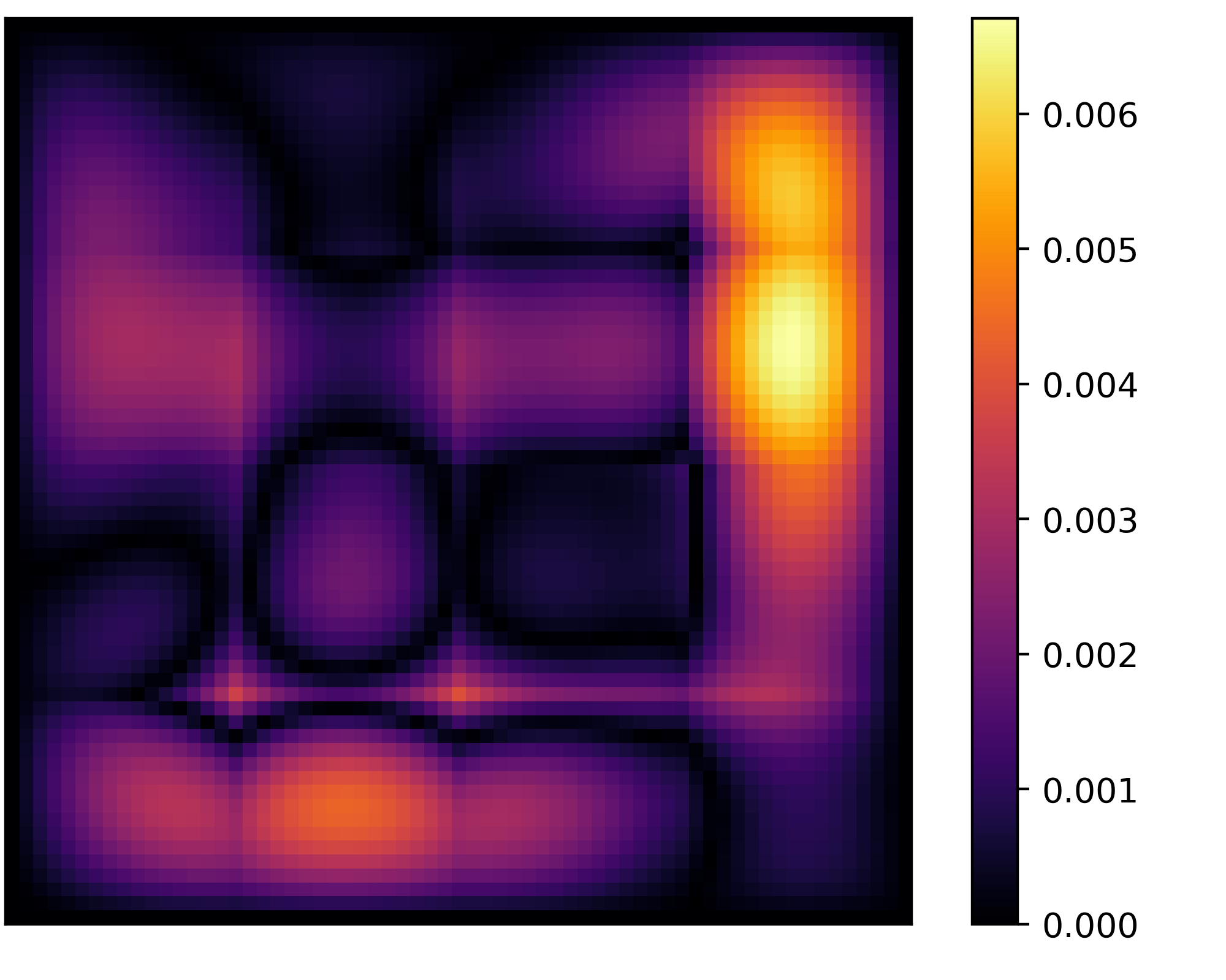
XXXXXXXXXXFine Solution
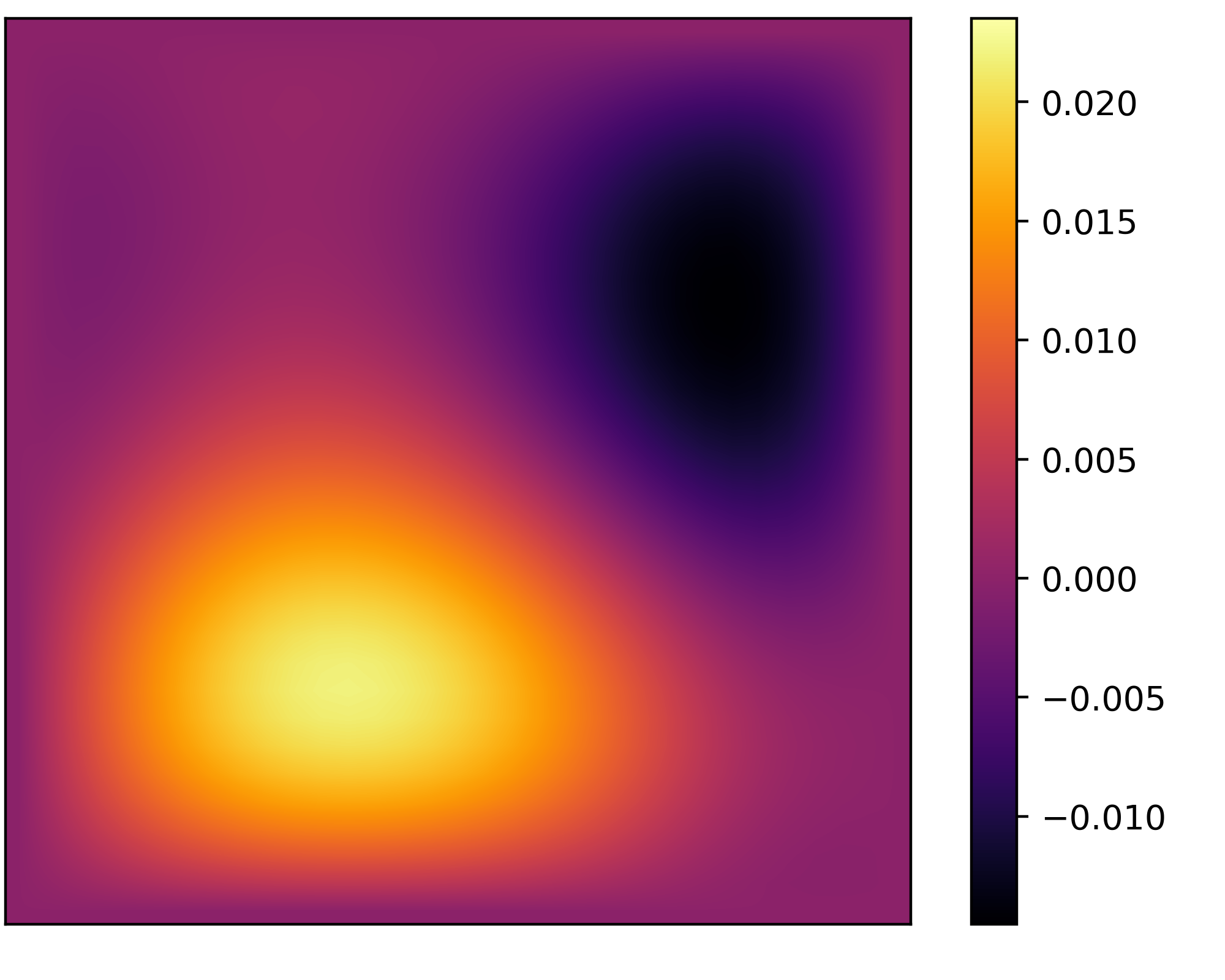
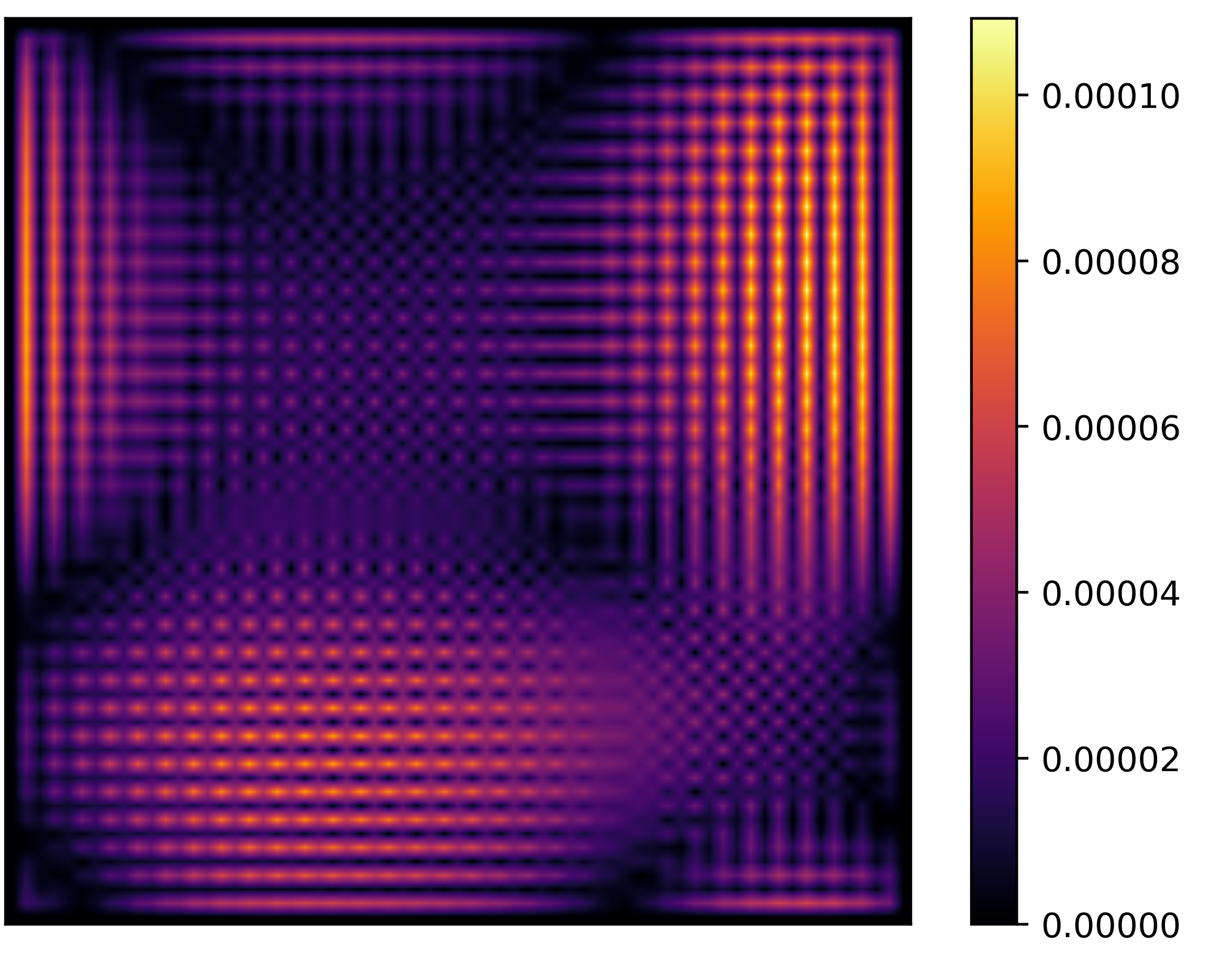
XXXXXXXXHybrid NN Solution

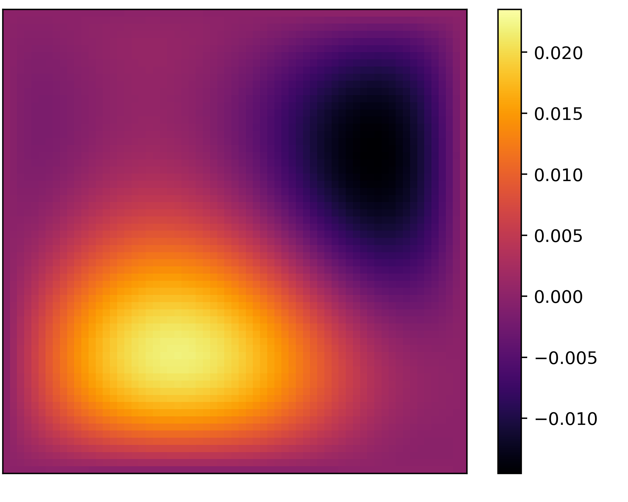
Figure 3: Performance of the hybrid finite element - neural network approach. Top: coarse mesh solution $u_{H}$ and error. Middle: resolved fine mesh solution $u_{h}$ and error. Bottom: hybrid finite element - neural network solution $u_{\cal N}$ and error.

Figure 3 shows an example of coarse, fine and network solution for a particular right hand side from the test data. Here we observe, that the quality of the network solution is significantly better than the quality of the original coarse solution.

References

- [1] N. Margenberg, D. Hartmann, C. Lessig, and T. Richter. A neural network multigrid solver for the navier-stokes equations. Journal of Computational Physics, 460:110983, 2022.
- [2] M. Raissi, P. Perdikaris, and G.E. Karniadakis. Physics-informed neural networks: A deep learning framework for solving forward and inverse problems involving nonlinear partial differential equations. Journal of Computational Physics, 378:686–707, 2019.
- [3] W. E and B. Yu. "the deep ritz method: A deep learning-based numerical algorithm for solving variational problems". Communications in Mathematics and Statistics, 6(1):1–12, 2018.
- [4] Peter L Bartlett, Dylan J Foster, and Matus J Telgarsky. Spectrally-normalized margin bounds for neural networks. Advances in neural information processing systems, 30, 2017.
- [5] Diederik P. Kingma and Jimmy Ba. Adam: A method for stochastic optimization. In International Conference on Learning Representations (ICLR), 2015.