Fixing confirmation bias in feature attribution methods via semantic match

Abstract

Feature attribution methods have become a staple method to disentangle the complex behavior of black box models. Despite their success, some scholars have argued that such methods suffer from a serious flaw: they do not allow a reliable interpretation in terms of human concepts. Simply put, visualizing an array of feature contributions is not enough for humans to conclude something about a model’s internal representations, and confirmation bias can trick users into false beliefs about model behavior. We argue that a structured approach is required to test whether our hypotheses on the model are confirmed by the feature attributions. This is what we call the “semantic match” between human concepts and (sub-symbolic) explanations. Building on the conceptual framework put forward in Cinà et al. [2023], we propose a structured approach to evaluate semantic match in practice. We showcase the procedure in a suite of experiments spanning tabular and image data, and show how the assessment of semantic match can give insight into both desirable (e.g., focusing on an object relevant for prediction) and undesirable model behaviors (e.g., focusing on a spurious correlation). We couple our experimental results with an analysis on the metrics to measure semantic match, and argue that this approach constitutes the first step towards resolving the issue of confirmation bias in XAI.

1 Introduction

The success of machine learning techniques in solving a variety of tasks, along with a parallel surge in model complexity, has rekindled interest in the interface between humans and machines. The field of Explainable AI (XAI henceforth) is concerned with unpacking the complex behavior of machine learning models in a way that is digestible by humans [Doshi-Velez and Kim, 2017, Linardatos et al., 2020, Gilpin et al., 2018, Biran and Cotton, 2017, Doran et al., 2017].

Among several proposed solutions, one approach has risen to prominence in the last half decade, namely what is known as feature attribution or feature importance. Loosely speaking, feature attribution methods explain machine behavior by indicating the extend to which different parts of the input contribute to the model’s output. It is hard to overstate how widespread such methods are: they are currently employed in a plethora of scenarios, including virtually all data modalities, and deployed in production in low- as well as high-risk environments [Thoral et al., 2021].

Yet, such techniques are not free from criticism. Beside doubts about consistency between explanations and faithfulness to the model, scholars have argued that feature attribution techniques expose the users of machine learning applications to confirmation bias, namely the reasoning pitfall that leads us to believe an explanation just because it aligns with our expectations [Lipton, 2018, Ghassemi et al., 2021]. For instance, a clinician using AI to diagnose metabolic disorders from images – after inspecting some explanations highlighting build-ups of fat in the liver – might be prone to believe that the model has learned to pay attention to fatty liver. As fatty liver is a known metabolic condition, the clinician will recognize it and possibly assume the machine recognizes it too. This may influence the level of trust the clinician has in the model, affecting the way care is delivered. But how can we be sure the model has learned this?

More generally, due to the sub-symbolic nature of feature attributions (i.e., the fact that they are just strings or matrices of numbers), we currently have no systematic way to ascertain whether explanations capture a concept we are interested in. Some authors advocate checking explanations against human intuition [Neely et al., 2022], but this exercise must be structured in a way that allows us to measure alignment between human concepts and explanations, lest we fall back into the problem of confirmation bias.

In this article, we build on the framework of semantic match proposed by Cinà et al. [2023] and formalize a procedure that allows us (1) to formulate a hypothesis with the form “the model behaves in this way”, and (2) to obtain a score representing the extent to which the model’s explanations confirm or reject this hypothesis. Such procedure is general and can in principle be applied to any model and to any local feature attribution method. In this article, we focus on SHapley Additive exPlanations (SHAP) [Lundberg and Lee, 2017] due to their widespread use in practice. Such a procedure is paired with a discussion on what metrics are appropriate to measure semantic match. We display the procedure in two sets of experiments on tabular and image data. We investigate different kinds of hypotheses about model behavior, showing that the procedure can give insight both into desirable behaviors – what we hope the model is doing well – as well as undesirable behaviors. All experiments use publicly available data and are fully reproducible.

2 Related Work

Feature attribution methods in XAI.

The majority of attribution-based methods provide local explanations, i.e., they aim to explain the prediction for an individual instance rather than the model as a whole and henceforth we focus our work on attribution-based methods (agnostic or specific) for local explainability. We can further break down attribution-based methods into gradient-based and perturbation-based methods. The former category includes, for instance, DeConvNet [Zeiler and Fergus, 2014], guided backpropagation (GBP) [Springenberg et al., 2014], Grad-CAM [Selvaraju et al., 2017], and integrated gradients [Sundararajan et al., 2017]. Methods that fall in the second category include Occlusion sensitivity maps [Zeiler and Fergus, 2014], LIME [Ribeiro et al., 2016a] and SHAP [Lundberg and Lee, 2017]. We refer to review papers such as those of Abhishek and Kamath [2022] and Singh et al. [2020] for a more detailed account of the different methods.

Criticism of feature attribution methods.

Although feature attribution methods are the most studied and deployed in practice [Bhatt et al., 2020], they are facing several criticisms. First, feature attribution methods do not produce stable results. They have been shown to be sensitive to adversarial perturbations that are perceptively indistinguishable and to produce drastically different results for similar inputs [Gan et al., 2022, Ghorbani et al., 2019, Slack et al., 2020]. For perturbation-based methods, due to sampling, two independent runs can result in different attributions [Gan et al., 2022]. These concerns have been studied in the literature and different approaches to tackle robustness and reliability have been proposed [e.g., Gan et al., 2022, Nielsen et al., 2022, Kindermans et al., 2019, Ghorbani et al., 2019, Adebayo et al., 2018]. Second, the methods tend to be sensitive to the choice of baseline, i.e., the reference values that feature importance scores are compared to [Haug et al., 2021, Sturmfels et al., 2020]. Third, the features deemed most important differ between methods for the same input. For example, Saarela and Jauhiainen [2021] compare the results obtained from logistic regression, random forest, and LIME [Ribeiro et al., 2016b] applied to both models and observe that different features are detected with these methods. Neely et al. [2022] compare the rank correlation between feature attribution methods and attention-based methods and find that there is no strong correlation between those methods. In general, there have been concerns about the performance of attribution-based methods, especially due to a lack of some ground truth for (quantitative) evaluation [Zhou et al., 2022].

Confirmation bias in XAI.

Confirmation bias is a well-known concept from psychology, first described by Wason [1960], and followed by plenty of empirical studies to investigate this phenomenon [e.g. Lord et al., 1979, Evans, 1989, Nickerson, 1998]. The American Psychological Association defines confirmation bias as “the tendency to gather evidence that confirms preexisting expectations, typically by emphasizing or pursuing supporting evidence while dismissing or failing to seek contradictory evidence” [American Psychological Association, n.d.]. Even though the literature on human cognition including confirmation bias is rich and the problem of this type of cognitive bias has been acknowledged in the (X)AI literature [e.g., Ghassemi et al., 2021, Cinà et al., 2023, Rudin, 2019], the empirical research on confirmation bias in XAI is scarce. Wang et al. [2019] propose a conceptual framework for building human-centered and decision-theory-driven XAI, in which they consider human decision making and the role of confirmation bias in relation to XAI. Wan et al. [2022] conducted a field experiment in which the study subjects were tasked with performing risk assessments aided by a predictive model, while Bauer et al. [2023] conducted two studies in the real estate industry investigating how humans shift their mental models. Both results find that confirmation bias is present in human-XAI interaction.

The risk of falling prey to confirmation bias is especially present if we use feature attribution methods on high-level features [Cinà et al., 2023]. Especially known from the field of computer vision and deep learning, high-level features refer to patterns in groups of features, while low-level features are the entries of the input vector [e.g., Zeiler and Fergus, 2014, Lee et al., 2016, Deng and Chen, 2014, Cinà et al., 2023]. Cinà et al. [2023] argue that the meaning of feature attributions for low-level features is intuitive, if the low-level features have a predefined semantic translation. This is the case in most tabular data structures, where every features has a concrete meaning. In image data, however, individual pixels do not carry any semantic meaning and hence the use of feature attribution methods is not sensible unless we know whether the high-level features match our semantic representation, i.e., if we have semantic match [Cinà et al., 2023, Kim et al., 2018].

Related approaches.

To our knowledge, there has been little work to check whether (something like) semantic match is present. In natural language processing an approach that is similar in spirit is probing classifiers, which is a way of understanding whether a language model’s internal representation is encoding some linguistic property Belinkov [2022]. Despite the shared intention to unpack sub-symbolic representations, model embeddings are not explanations and probing does not appeal to intuitions in the same way as feature attribution methods do. In image classification, a typical approach to explain the classification is using prototypes. Essentially, the explanation relies on ‘this looks like that’ reasoning and provides prototypical images from the training data to explain some classification [e.g., Arik and Pfister, 2020, Biehl et al., 2016, Nauta et al., 2021]. In Nauta et al. [2021], this idea is extended by explaining in what visual aspects, such as color hue, saturation, shape, texture, and contrast, the test image is similar to the prototype. They quantify the influence of these aspects in a prototype and by that clarify the classification of the test image. Another approach for interpretable image classification is concept-based models or concept bottleneck models (CBMs) [e.g., Kim et al., 2018, Barbiero et al., 2022, Yuksekgonul et al., 2022, Ghosh et al., 2023]. The core idea of such approaches is to map inputs onto some user-defined concepts, which are then used to predict the outcome class. In both CBMs and prototype explanations, the intention is to ground explanations by latching them to concepts or prototypes for which semantic match is given.

Contributions.

We propose an approach to test directly whether semantic match is present for the hypotheses that we are interested in, without the need of pre-defined concepts or prototypes. Our metrics for semantic match can also support a quantitative analysis of model behavior, and when semantic match is not achieved, we can side-step our intuition and thus avoid confirmation bias.

3 Methodology

In this section we describe the main methodology in full generality and elaborate on the metrics to assess semantic match. We also outline the setup of the experiments on tabular and image data.

3.1 Main procedure

Consider a dataset with input vectors $X=\{x_{1},x_{2},\dots,x_{n}\}$ and the corresponding output labels $Y=\{y_{1},y_{2},\dots,y_{n}\}$. Thus, the data point $i$ is denoted by the pair $(x_{i},y_{i})\in X\times Y$. We assume that a machine learning (ML) model $f$ has been trained on this dataset and a local feature attribution method $M$ is specified. The term $M(f,x_{i},y_{i})=e_{i}$ defines the explanation $e_{i}$ obtained by $M$ for data point $i$ that is classified with model $f$.

When evaluating semantic match, we consider a specific sample $x_{c}\in X$ and a corresponding explanation $e_{c}$. We are interested in testing whether we have semantic match with the explanation $e_{c}$, or in other words, whether what we ‘see’ in the explanation is indeed what the explanation is capturing. At an intuitive level, what we want to ascertain is that an explanation matches our translation of it. This is encoded in the commutation of the semantic diagram from Cinà et al. [2023], namely that all the data points giving rise to a certain explanation are also complying with our translation hypothesis, which we will indicate with $\theta$, and vice versa. Mathematically this can be written as

$$\{x\in X~{}|~{}M(f,x,y)\approx e_{c}\}=\{x\in X~{}|~{}(x,y)\models\theta\},$$ (1)

where $(x,y)\models\theta$ denotes that the corresponding data point complies with the hypothesis $\theta$. Note that we expect our reference point $x_{c}$ to comply with $\theta$, since it is the explanation $e_{c}$ that elicited it. We propose a procedure to test how much such equality holds in a practical case. The procedure requires a distance metric between explanations, which we will denote as $d$, a maximum distance allowed $\epsilon$, a number of samples $n$, and a method to test a hypothesis $\theta$ on data points. In case of explanations as vectors or matrices, there are standard notions of distance to employ; see Section 4 for several examples. The choices of $\epsilon$ and $n$ depend on how thorough an inspection one wants to conduct. We thus rewrite the test as

$$\underset{X^{\epsilon}}{\underbrace{\{x\in X~{}|~{}d(M(f,x,y),e_{c})\leq\epsilon\}}}=\underset{X^{\theta}}{\underbrace{\{x\in X~{}|~{}(x,y)\models\theta\}}}$$ (2)

where the left-hand side is a set containing all data points generating an explanation close to $e_{c}$ (subset $X^{\epsilon}$), and the right-hand side is a set containing all data points satisfying $\theta$ (subset $X^{\theta}$).

To exemplify the procedure, suppose one has developed an algorithm to classify pictures of animals. Presented with a picture of a dog and an explanation $e_{c}$, one may formulate the translation hypothesis $\theta$ that the explanation highlights the tail of the dog. Following the procedure, one would first obtain a dataset with input images and explanations, and then identify the images with explanations sufficiently similar to $e_{c}$ (i.e., subset $X^{\epsilon}$), as well as the images that contain tails (i.e., subset $X^{\theta})$. It is then possible to evaluate the overlap between these two sets. Note that, while our algorithm uses a single dataset for both $X^{\epsilon}$ and $X^{\theta}$, it would also be possible to obtain separate samples for these two sets. For example, one can consider the use of generative models to generate samples satisfying $\theta$, and evaluating the the similarity of the explanations obtained for this set compared to $e_{c}$.

3.2 Metrics for semantic match

We now turn our attention to quantifying the semantic match. Since we have defined distances in terms of a reference point, each of the metrics defined in this section will have to be re-computed by sampling data points within $X_{\theta}$ to understand how much the results depend on the choice of data point. Our two tests boil down to two questions: (1) how necessary is $\theta$ for an explanation similar to $e_{c}$, and (2) how sufficient is $\theta$ for an explanation similar to $e_{c}$? In proportion/probability notation, for some random input $x_{i}\in X$, we define

$$q_{1}=P\left(x_{i}\in X^{\theta}|x_{i}\in X^{\epsilon}\right)\quad\text{and}\quad q_{2}=P\left(x_{i}\in X^{\epsilon}|x_{i}\in X^{\theta}\right).$$ (3)

These two metrics effectively offer two perspectives on the overlap between the area defined by $\theta$ and the area defined by setting a threshold $\epsilon$ on the distances. One drawback of these quantities is that they are threshold-dependent, and the choice of threshold is somewhat arbitrary. An alternative way to test for semantic match is to think about the distances of the explanations from $e_{c}$ as constituting a ranking of the data points. This ranking can then be used to ‘predict’ which data points satisfy $\theta$.

Semantic match as classification.

Using the training dataset, we construct a new dataset by relabeling the samples using the hypothesis $\theta$. That is, we obtain new labels with $\theta$ by defining

$$\bar{y}_{i}=\mathds{1}\big{(}(x_{i},y_{i})\models\theta\big{)},\quad i=1,\dots,n.$$ (4)

Here, $\mathds{1}$ stands for the indicator function. In other words, a sample is relabeled as one if it complies with the hypothesis; otherwise, its label is zero. Given the machine learning model $f$, the local feature attribution method $M$ and explanation $e_{c}$, we can also construct ‘predictions’ as follows:

$$h_{c}(x_{i})=\mathds{1}\big{(}d(M(f,x_{i},y_{i}),e_{c})\leq\epsilon\big{)},$$ (5)

In light of this construction, the metrics in Eq. (3) are the precision and recall values, respectively. When considering the distances as a ranking, we need to flip the sign since in our case smaller distances are supposed to indicate higher chance of satisfying $\theta$, while in standard classification problems larger values are supposed to indicate the positive class. With this approach, we can resort to well-known metrics to measure the discrimination of rankings, such as the area under the ROC curve (shortened with AUC): for every threshold on the distance we can obtain a value of true positive rate and true negative rate, and vary the threshold to obtain the standard AUC plot.

Coherence of explanations.

Obtaining a high AUC for semantic match indicates that explanations allow us to separate the points satisfying $\theta$ from those that do not. However, AUC is invariant to monotone transformations and does not indicate how coherent explanations are with each other. In case of global behavior of the model (e.g., is the model placing attention on the object to classify), we are also interested in measuring the consistency between $\theta$ and explanations (for this dataset, these explanations and this model), not just on discrimination. In order to measure the coherence among explanations, we resort to the median distance of all explanations from the reference point $e_{c}$, to understand how much explanations cluster close to the $\theta$ region.

3.3 Experimental setup

For the sake of simplicity, we limit our experiments to a single explanatory technique and opted for SHAP values Lundberg and Lee [2017], since it is a widely used technique that is easily applicable across data modalities.

Experiments on tabular data.

To illustrate the procedure to test semantic match, we first design a controlled experiment on synthetic data. We want to control the data generating process and have clarity on what is the high-level feature the model may be picking up, so that we can have clear expectations on whether semantic match should work or not.

We generated a tabular dataset consisting of two continuous features normally distributed, $x_{1}$ and $x_{2}$, and one binary feature $x_{3}$. We proceeded to define a binary outcome by passing the function $x_{1}x_{3}--(1-x_{3})x_{1}+x_{2}$ through a sigmoid and a 0.5 threshold. In this way, we incorporate a feature interaction between features $x_{1}$ and $x_{3}$ into the outcome; this will be the high-level feature of interest. We then trained a random forest on the dataset in order to predict the outcome from the three features, and generated explanations using SHAP. In principle, the random forest algorithm should be able to pick up on such feature interaction.

Next, we wanted to use explanations to understand whether the model had learned about the feature interaction. We picked a data point $x_{c}$ with negative $x_{1}$ value and $x_{3}=0$, whose explanation $e_{c}$ gave positive contribution for both these features. We formulated the following hypothesis $\theta$: “the model has learned that $x_{3}=0$ flips the effect of $x_{1}$ and thus increase the probability of the outcome when $x_{1}$ is negative and $x_{3}=0$”. We operationalized $\theta$ by considering the subset of the data where $x_{1}<0$ and $x_{3}=0$: this is the subset of data points for which – if semantic match is achieved – we expect explanations to be close to $e_{c}$. Finally, we define a notion of distance between explanations. We opted for Euclidean distance between vectors of SHAP values and deemed two explanations to be ’similar’ whose distance was below a threshold $\epsilon$, which we tested at different values. With these ingredients we are then able to test for semantic match.

Experiments on images.

We further experimented on a computer vision task from the literature with the goal of assessing semantic match for vision-related hypotheses. We employed data from MALeViC [Pezzelle and Fernández, 2019], a dataset of synthetically-generated images depicting four to nine colored geometric objects with varying areas. The objects are generated at random locations in the images. Since MALeViC was originally introduced to study an object’s contextually-defined size, each shape has a corresponding binary label – big or small – which stands for its size in the context of the whole image, i.e., whether it counts as big or small given the surrounding objects. These are based on an underlying threshold function considering the area occupied by the objects. For each image, the threshold $T$ is computed as follows: $T(I)=Max--k(Max-Min)$, where $I$ is the image, $k$ is randomly sampled from the normal distribution of values centered on $0.29$ ($\mu=0.29$, $\sigma=0.066$), and $Max$ and $Min$ are the areas, in pixels, of the biggest and smallest objects in $I$, respectively. During the construction of the dataset, an object is deemed big if its area exceeds $T$; otherwise, small. To solve this task, a model will need to construct high-level features capturing the role of the target object and the relationship with the other shapes.

Here, we focus on the partition of the MALeViC dataset where all the objects in an image are either squares or rectangles. This choice has a practical motivation, namely to have a direct mapping between objects and their bounding boxes. Furthermore, we select images that contain one single red object. The resulting dataset is balanced in terms of objects’ sizes. We split our dataset into training, validation and test sets (80:10:10). To augment our training data, we flip each image horizontally and vertically. Thus, we end up with 4800 images in the training set and 200 images in the test set. We trained a model to predict whether red objects are big or small. The model is a convolutional neural network (CNN) that takes the three-channel input images and outputs a probability over the two classes (small or big). Further details on the implementation are specified in Appendix B.

We generate explanations by obtaining pixel-level SHAP values. It is difficult to compare heatmaps directly because the shapes spawn at random locations in the images. The MALeVIC dataset comes equipped with metadata on the location of the bounding box for each shape in an image. After segmenting the whole image with Segment Anything Model (SAM) [Kirillov et al., 2023], we are able to identify the relevant masks by matching their coordinates to the coordinates of the relevant bounding boxes using the metadata. This allowed us to consider only the SHAP values of the pixels inside a certain shape, as depicted in Figure 1.

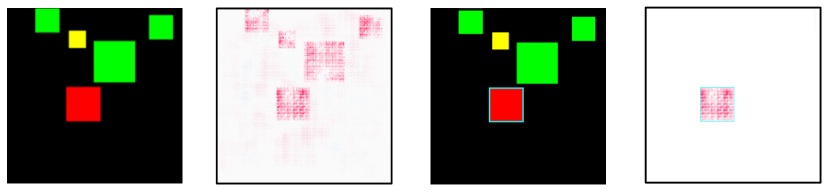
Figure 1: An example image from the MALeViC dataset (left), alongside the SHAP values generated by the model (center-left), the cyan bounding box around the object of interest (center-right) and the SHAP values after masking is applied (right).

All the hypotheses considered concern the contribution placed on the target red object. Thus, we calculate the amount of SHAP values placed on the relevant shape using the bounding box as a mask on the SHAP heatmap. We add up the absolute value of the contribution of the pixels within the bounding box and normalize this quantity by the total contribution in the whole image. This gives us the proportion of the attention placed on the target object in the reference image $x_{c}$. Given any other image, we will calculate the proportion of contribution of the red shape with the same method, and measure the distance as the absolute difference in these proportions. Therefore, if our reference explanation places 40% of the contribution on the red object and in another image the contribution of the red object is 10%, the distance between the two explanations is 30% or 0.3. In this way, we have a notion of distance that is only considering the relevant parts of the images and is not affected by the fact that shapes can be located in different places.

4 Results

We summarize our results in the two sets of experiments.

4.1 Synthetic experiments on tabular data

On this simple task, the model has an AUC of 1.00, thus it must have learned about the feature interaction. Our experiment was geared towards testing whether the explanations matched our hypothesis “the model has learned that $x_{3}=0$ flips the effect of $x_{1}$ and thus increase the probability of the outcome when $x_{1}$ is negative and $x_{3}=0$”.

By choosing a first data point as a point of reference, we obtained a semantic match AUC of 0.99 and a median distance of 0.20. This indicates that the distances allow us to distinguish data points where the first feature is negative and the third is zero, but explanations are not coherent. Inspection of the histogram of distances of the explanations (Figure 2, blue histogram) reveals a group of data points for which the distance is rather large. What is at play here is that $x_{2}$ is confounding our notion of distance: while $x_{2}$ is irrelevant for the hypothesis we formulated, our naive notion of distance does take into account the distance on that dimension too. This simple example brings into light the fact that hypotheses may be local. Revising our notion of distance to only consider dimension $x_{1}$ and $x_{3}$, we see a drop in median distance reaching 0.09, while semantic match AUC remains high at 0.92. We also observe in the orange histogram of Figure 2 a shape that complies with expectations: explanations cluster close to $e$, with fewer and fewer examples as we allow for more distance.

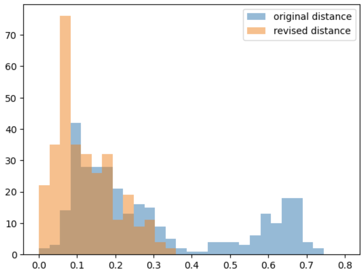
Figure 2: For the data points in the subspace defined by $x_{1}<0$ and $x_{3}=0$, we are interested in checking how similar the explanations are with respect to to $e_{c}$. We visualize this as a histogram with the distance on the horizontal axis. Refining the notion of distance to one that is hypothesis-driven, we remove the “noise” introduced by $x_{2}$ and ascertain that the explanations of the relevant data points do cluster in the vicinity of $e_{c}$.

These observations allow us to conclude that we have a reasonable level of semantic match, and thus we are confident that the explanations reveal what our hypothesis has described. Note that in this process we have not dissected the model itself, which in principle has remained a black box. We elaborate on the robustness of these results in Appendix A.

4.2 Experiments on images

On the MALeViC dataset, the model reached an accuracy of 91.5% on the classification task. We were thus interested in confirming the model has learned which shapes it is supposed to consider, a theory that is also suggested by visual inspection of some explanations. We formulated various hypotheses regarding the contribution placed on specific objects in the image. Notably, the distance between reference explanations ($e_{c}$) and all explanations expresses a difference in percentage of attention placed on the objects of interest. First, we studied the amount of contribution placed on the target object and the correctness of the model’s predictions by formulating the following hypotheses:

• $\theta_{1}$: ‘$\geq 10\%$ of the attention is placed on the target object’

• $\theta_{2}$: ‘$\geq 10\%$ of the attention is placed on the target object and the prediction is correct’

• $\theta_{3}$: ‘$<5\%$ of the attention is placed on the target object and the prediction is correct’

• $\theta_{4}$: ‘$<5\%$ of the attention is placed on the target object and the prediction is not correct’

The results are summarized in Figure 3. Hypotheses $\theta_{1},\theta_{2},\theta_{3},\theta_{4}$ all obtain high AUC, suggesting the explanations clearly separate the data points complying to the hypotheses from the rest. Overall, the median distances are relatively small (i.e., the median of median distances stands close to 6%). This suggests that, for all explanations, variability is relatively low compared to the reference points. In particular, since the reference points for hypotheses $\theta_{3},\theta_{4}$ have less than 5% of contribution placed on the target objects, this entails that all explanations put little attention on the target object. We can thus conclude that semantic match for those hypotheses is high and therefore the model does not behave as desired, i.e., focus on the target object. For further insights into the semantic match on the hypotheses considered, we refer the reader to Appendix B.

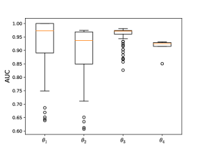
((a)) AUC boxplots

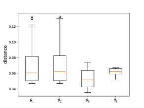
((b)) median distance boxplots

Figure 3: Boxplots of the two main metrics (i.e., AUC and median distance) to assess semantic match for hypotheses based on attention placed to red target object in images from the MALeVIC dataset. The boxplots are obtained by sampling all data points complying with the hypothesis as points of reference.

If the focus on the target object does not explain the high performance of the model, perhaps the model is using the smallest and largest object to perform the classification (see Section 3 for explanations on the data generation). Therefore we formulated a similar set of hypotheses, expanding their scope to encompass the contribution placed on the triple of the target, biggest and smallest objects in the image:

• $\theta_{5}$: ‘$\geq 30\%$ of the attention is placed on the target, biggest and smallest objects’

• $\theta_{6}$: ‘$\geq 30\%$ of the attention is placed on the target, biggest and smallest objects and the prediction is correct’

• $\theta_{7}$: ‘$<15\%$ of the attention is placed on the target, biggest and smallest objects and the prediction is correct’

• $\theta_{8}$: ‘$<15\%$ of the attention is placed on the target, biggest and smallest object and the prediction is not correct’

The results are summarized in Figure 4. Notably, the trends are similar to the ones observed in the previous set of hypothesis. Hypotheses $\theta_{5},\theta_{6},\theta_{7},\theta_{8}$ all also obtain high AUC (albeit the first two with high variability), suggesting that explanations complying with the hypothesis and those which do not can be separated easily. The AUC distributions for this set of hypotheses is broadly comparable to the ones observed in hypotheses $\theta_{1},\theta_{2},\theta_{3},\theta_{4}$, respectively. Overall, the median distances are small (i.e., roughly between 10% and 20%), although slightly larger than in the previous set of hypotheses. Overall, the budget of contribution devoted to the biggest, smallest and target object tends to be less than half. This indicates that there are more factors playing a role for the model to come up with a decision. Since the target, smallest and largest objects should be the only objects affecting the classification, this results strongly suggests that the model is utilizing some spurious correlation. Further insights into semantic match on the hypotheses considered can be found in the Appendix B.

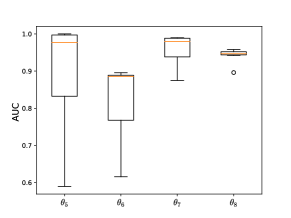
((a)) AUC boxplots

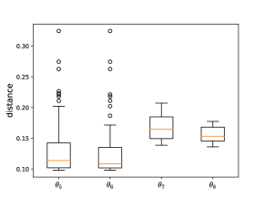
((b)) median distance boxplots

Figure 4: Boxplots of the two main metrics (i.e., AUC and median distance) to assess semantic match for hypotheses based on attention placed to red target, biggest and smallest objects in images from the MALeVIC dataset. The boxplots are obtained by sampling all data points complying with the hypothesis as points of reference.

5 Discussion

In the previous sections, we laid out a procedure to investigate the semantic match between human-understandable concepts and attribution-based explanations. The procedure begins in a way that is akin to how such explanations are commonly used: by examining a data point with its explanation, and formulating a hypothesis on what the model has learned. We showed how this first step can continue by making the hypothesis more precise, and by defining a notion of distance between explanations that is hypothesis-driven. We then proposed some diagnostic tools to measure the level of semantic match between said hypothesis and the explanations. Such numerical analysis of the explanations can ground our intuitions and prevent confirmation bias.

This framework was put to the test on synthetic tabular data and on a computer vision task on the MALeViC dataset. We observed how, without any prior knowledge about the model, the semantic match framework allows us to draw conclusions about model behavior. In the computer vision task, we started by investigating a desirable behavior, and concluded that the model was behaving in an undesirable way (i.e., not placing enough attention to the relevant shapes). Such experiments, while revealing the complexity of the problem, showcase that this framework can elicit useful information on model behavior and prevent confirmation bias.

When it comes to limitations of this approach, it should be noted that this whole endeavor is predicated on the assumption that explanations have some degree of faithfulness to the model [Jacovi and Goldberg, 2020]. If explanations misrepresent the model, a semantic match between our ideas and the explanations is not going to give us information about the model. Moreover, we only experimented with SHAP, which is but one of the many feature attribution techniques available; it remains to be shown that this framework also generalizes to other explainability techniques.

Furthermore, the experiments revealed several interesting aspects of semantic match. First, hypotheses are often local, in the sense that they pertain to a part of the input data, and it may not be straightforward to define a relevant notion of distance between explanations (see for example the bounding box problem in Section 3.3). Second, perhaps unsurprisingly, the results we obtained were sensitive to the specification of the hypothesis, highlighting the importance of formalizing hypotheses precisely and testing different specifications. Third, we find that sharpening the hypothesis does not necessarily lead to crisper results, see for instance $\theta_{1}$ and $\theta_{2}$ from the set of image experiment in Figure 3. More generally, the role of the logical structure of the hypotheses remains to be investigated; the divergent AUCs values for $\theta_{3}$ and $\theta_{4}$ from the set of image experiments in Figure 3 might be related to fact that $\theta_{4}$ contains a negation of a term of $\theta_{3}$.

In future work, we plan on expanding the suite of experiments further, tackling more real-world tasks and datasets, as well as expand to other feature attribution methods. We also intend to formalize more precisely a language for posing hypotheses, in the vein of a query language, so that the process of testing semantic match can be further refined and automatized.

Appendix A Expanded results on synthetic tabular data

The simulation reported in 3.3 was repeated adding a noise factor $k$ to the outcome, to assess robustness of semantic match in light of noisy outcomes. More specifically, the baseline function that was passed through a sigmoid was changed to $x_{1}x_{3}--(1-x_{3})x_{1}+x_{2}$ to $x_{1}x_{3}--(1-x_{3})x_{1}+x_{2}+kx_{4}$, where $k$ is a chosen constant and $x_{4}$ is a standard normal variable (such as $x_{1}$ and $x_{2}$). Thus, a value of $k=0.5$ leads to a noise impact on the model of around half the impact of $x_{2}$. Simulations with different combinations of $\epsilon$ and $k$ – with the same $\theta$ and sample size $N=1000$ – give the expected results (where $q_{1r}$ and $q_{2r}$ are the metrics calculated with the revised distance including only features $x_{1}$ and $x_{3}$); we display here some examples:

• $\epsilon=0.05$, $k=0$: $q_{1}=1.0$, $q_{1r}=0.84$, $q_{2}=0.025$, $q_{2r}=0.1338$.

• $\epsilon=0.05$, $k=0.5$: $q_{1}=0.5833$, $q_{1r}=0.5745$, $q_{2}=0.02229$, $q_{2r}=0.0860$.

• $\epsilon=0.2$, $k=0$: $q_{1}=0.6633$, $q_{1r}=0.5299$, $q_{2}=0.4204$, $q_{2r}=0.7898$.

• $\epsilon=0.2$, $k=0.5$: $q_{1}=0.5735$, $q_{1r}=0.5009$, $q_{2}=0.5096$, $q_{2r}=0.8694$.

As the distance constitutes a reverse ranking (smaller distances should mean higher chance to fulfill the hypothesis), larger threshold $\epsilon$ means lower proportion $q_{1}$ (precision) and higher proportion $q_{2}$ (recall). In other words, the larger $\epsilon$, the less similar explanations become, and $P(x_{i}\in X^{e})$ converges to 1. On the other hand, the larger the threshold the more $q_{1}$ (precision) tends towards $P(X^{\theta})$. This is displayed clearly in plots such as Figure 7(d) and LABEL:fig:text_q1q2. The noise appears to worsen semantic match – and performance on the downstream task – but these trends remain.

Appendix B Expanded results on the MALeViC data

The input for the convolutional neural network is a 3-channel image containing squares or rectangles. The model used consists of three convolutional layers with 3,16 and 32 filters respectively. The dimension of the filters is 3x3. Each convolutional layer is followed by max pooling (2x2 filter) and a ReLU activation function. The output is flattened and passed through a dropout layer (25% rate), two fully connected layers and a sigmoid to output probabilities. The overall architecture is shown in Figure 5. The network was trained for 20 epochs using a batch size of 128. The chosen optimization algorithm was Adam with a learning rate set to 0.001 using the binary cross entropy loss. The random seed is set to 42. During training, the model with lowest validation loss was selected for inference.

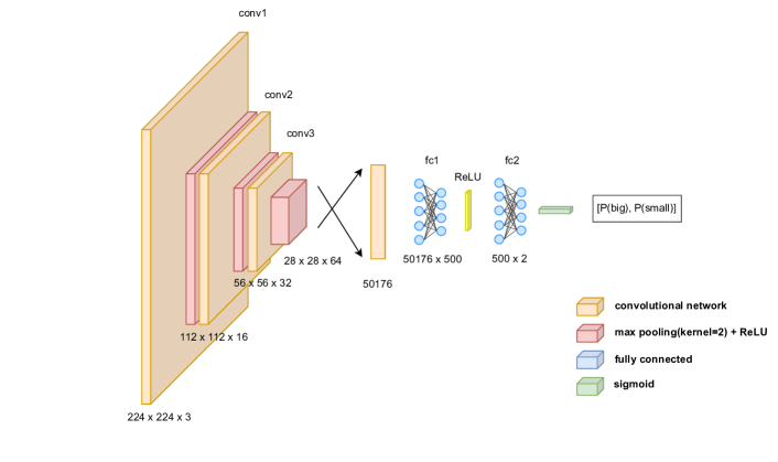
Figure 5: CNN Architecture

We report in Figures 6(h) the histograms of the distances and in Figure 7(d) the precision-recall curves for the four hypotheses.

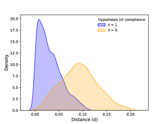
((a)) Distances for hypothesis $\theta_{1}$.

((b)) Distances for hypothesis $\theta_{2}$.

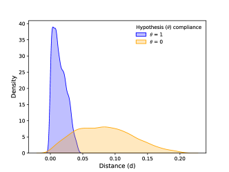
((c)) Distances for hypothesis $\theta_{3}$.

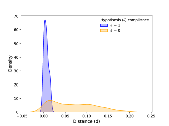
((d)) Distances for hypothesis $\theta_{4}$.

((e)) Distances for hypothesis $\theta_{5}$.

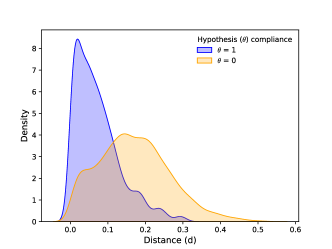
((f)) Distances for hypothesis $\theta_{6}$.

((g)) Distances for hypothesis $\theta_{7}$.

((h)) Distances for hypothesis $\theta_{8}$.

Figure 6: Kernel density estimate plot for distances between reference explanation percentage attention (e_c) and all explanations percentage attention (e_i) from the MALeVIC dataset. In blue, distances between e_c and e_i when $\theta$ = 1. In orange, distances between e_c and e_i when $\theta$ = 0.

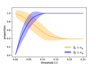
((a)) $q_{1}$ and $q_{2}$ curves for hypothesis $\theta_{1}$.

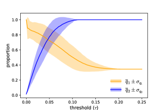
((b)) $q_{1}$ and $q_{2}$ curves for hypothesis $\theta_{2}$.

((c)) $q_{1}$ and $q_{2}$ curves for hypothesis $\theta_{3}$.

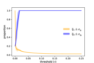
((d)) $q_{1}$ and $q_{2}$ curves for hypothesis $\theta_{4}$.

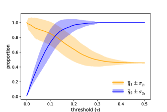
((e)) $q_{1}$ and $q_{2}$ curves for hypothesis $\theta_{5}$.

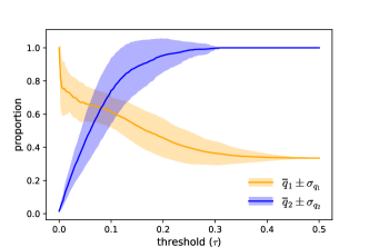
((f)) $q_{1}$ and $q_{2}$ curves for hypothesis $\theta_{6}$.

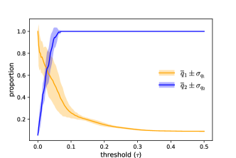
((g)) $q_{1}$ and $q_{2}$ curves for hypothesis $\theta_{7}$.

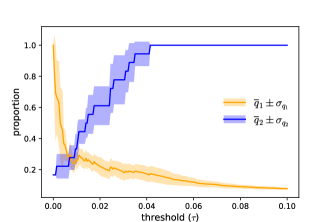
((h)) $q_{1}$ and $q_{2}$ curves for hypothesis $\theta_{8}$.

Figure 7: $q_{1}$ and $q_{2}$ curves (i.e., precision-recall curves) for datapoints from the MALeVIC dataset. In blue, $q_{1}$ curve. In orange, $q_{2}$ curve.

References

- Abhishek and Kamath [2022] K. Abhishek and D. Kamath. Attribution-based XAI methods in computer vision: A review. arXiv, 2022. URL https://arxiv.org/abs/2211.14736.
- Adebayo et al. [2018] J. Adebayo, J. Gilmer, M. Muelly, I. Goodfellow, M. Hardt, and B. Kim. Sanity checks for saliency maps. In S. Bengio, H. Wallach, H. Larochelle, K. Grauman, N. Cesa-Bianchi, and R. Garnett, editors, Advances in Neural Information Processing Systems, volume 31. Curran Associates, Inc., 2018. URL https://proceedings.neurips.cc/paper/2018/file/294a8ed24b1ad22ec2e7efea049b8737-Paper.pdf.
- American Psychological Association [n.d.] American Psychological Association. Confirmation bias, n.d. URL https://dictionary.apa.org/confirmation-bias.
- Arik and Pfister [2020] S. O. Arik and T. Pfister. Protoattend: Attention-based prototypical learning. Journal of Machine Learning Research, 21(1):8691––8725, jan 2020. ISSN 1532-4435. URL https://dl.acm.org/doi/abs/10.5555/3455716.3455926.
- Barbiero et al. [2022] P. Barbiero, G. Ciravegna, F. Giannini, P. Lió, M. Gori, and S. Melacci. Entropy-based logic explanations of neural networks. Proceedings of the AAAI Conference on Artificial Intelligence, 36(6):6046–6054, Jun. 2022. URL https://ojs.aaai.org/index.php/AAAI/article/view/20551.
- Bauer et al. [2023] K. Bauer, M. von Zahn, and O. Hinz. Expl(ai)ned: The impact of explainable artificial intelligence on users’ information processing. Information Systems Research, 0(0), 2023. URL https://doi.org/10.1287/isre.2023.1199.
- Belinkov [2022] Y. Belinkov. Probing classifiers: Promises, shortcomings, and advances. Computational Linguistics, 48(1):207–219, 04 2022. ISSN 0891-2017. URL https://doi.org/10.1162/coli_a_00422.
- Bhatt et al. [2020] U. Bhatt, A. Xiang, S. Sharma, A. Weller, A. Taly, Y. Jia, J. Ghosh, R. Puri, J. M. F. Moura, and P. Eckersley. Explainable machine learning in deployment. In Proceedings of the 2020 Conference on Fairness, Accountability, and Transparency, FAT* ’20, page 648–657, New York, NY, USA, 2020. Association for Computing Machinery. ISBN 9781450369367. URL https://doi.org/10.1145/3351095.3375624.
- Biehl et al. [2016] M. Biehl, B. Hammer, and T. Villmann. Prototype-based models in machine learning. WIREs Cognitive Science, 7(2):92–111, 2016. doi: https://doi.org/10.1002/wcs.1378. URL https://wires.onlinelibrary.wiley.com/doi/abs/10.1002/wcs.1378.
- Biran and Cotton [2017] O. Biran and C. Cotton. Explanation and justification in machine learning: A survey. IJCAI-17 Workshop On Explainable AI (XAI), 8(1):8—13, 2017. URL http://www.cs.columbia.edu/~orb/papers/xai_survey_paper_2017.pdf.
- Cinà et al. [2023] G. Cinà, T. E. Röber, R. Goedhart, and Ş. İlker. Birbil. Semantic match: Debugging feature attribution methods in xai for healthcare. arXiv, 2023. URL https://arxiv.org/abs/2301.02080.
- Deng and Chen [2014] L. Deng and J. Chen. Sequence classification using the high-level features extracted from deep neural networks. In 2014 IEEE International Conference on Acoustics, Speech and Signal Processing (ICASSP), pages 6844–6848, 2014. URL https://doi.org/10.1109/ICASSP.2014.6854926.
- Doran et al. [2017] D. Doran, S. Schulz, and T. R. Besold. What does explainable AI really mean? A new conceptualization of perspectives. arXiv, 2017. URL https://arxiv.org/abs/1710.00794.
- Doshi-Velez and Kim [2017] F. Doshi-Velez and B. Kim. Towards a rigorous science of interpretable machine learning. arXiv, 2017. URL https://arxiv.org/abs/1702.08608.
- Evans [1989] J. S. B. T. Evans. Bias in human reasoning: Causes and consequences. Lawrence Erlbaum Associates, Inc, 1989.
- Gan et al. [2022] Y. Gan, Y. Mao, X. Zhang, S. Ji, Y. Pu, M. Han, J. Yin, and T. Wang. "Is your explanation stable?": A robustness evaluation framework for feature attribution. In Proceedings of the 2022 ACM SIGSAC Conference on Computer and Communications Security, CCS ’22, page 1157–1171, New York, NY, USA, 2022. Association for Computing Machinery. ISBN 9781450394505. URL https://doi.org/10.1145/3548606.3559392.
- Ghassemi et al. [2021] M. Ghassemi, L. Oakden-Rayner, and A. L. Beam. The false hope of current approaches to explainable artificial intelligence in health care. The Lancet Digital Health, 3(11):e745–e750, 2021. ISSN 2589-7500. URL https://doi.org/10.1016/s2589-7500(21)00208-9.
- Ghorbani et al. [2019] A. Ghorbani, A. Abid, and J. Zou. Interpretation of neural networks is fragile. Proceedings of the AAAI Conference on Artificial Intelligence, 33(01):3681–3688, Jul. 2019. URL https://doi.org/10.1609/aaai.v33i01.33013681.
- Ghosh et al. [2023] S. Ghosh, K. Yu, F. Arabshahi, and K. Batmanghelich. Route, interpret, repeat: Blurring the line between post hoc explainability and interpretable models. arXiv, 2023. URL https://arxiv.org/abs/2302.10289.
- Gilpin et al. [2018] L. H. Gilpin, D. Bau, B. Z. Yuan, A. Bajwa, M. Specter, and L. Kagal. Explaining explanations: An overview of interpretability of machine learning. 2018 IEEE 5th International Conference on Data Science and Advanced Analytics (DSAA), 00:80–89, 2018. URL https://doi.org/10.1109/dsaa.2018.00018.
- Haug et al. [2021] J. Haug, S. Zürn, P. El-Jiz, and G. Kasneci. On baselines for local feature attributions. arxiv, 2021. URL https://arxiv.org/abs/2101.00905.
- Jacovi and Goldberg [2020] A. Jacovi and Y. Goldberg. Towards faithfully interpretable NLP systems: How should we define and evaluate faithfulness? In Proceedings of the 58th Annual Meeting of the Association for Computational Linguistics, pages 4198–4205, Online, July 2020. Association for Computational Linguistics. doi: 10.18653/v1/2020.acl-main.386. URL https://aclanthology.org/2020.acl-main.386.
- Kim et al. [2018] B. Kim, M. Wattenberg, J. Gilmer, C. Cai, J. Wexler, F. Viegas, and R. sayres. Interpretability beyond feature attribution: Quantitative testing with concept activation vectors (TCAV). In J. Dy and A. Krause, editors, Proceedings of the 35th International Conference on Machine Learning, volume 80 of Proceedings of Machine Learning Research, pages 2668–2677. PMLR, 10–15 Jul 2018. URL https://proceedings.mlr.press/v80/kim18d.html.
- Kindermans et al. [2019] P.-J. Kindermans, S. Hooker, J. Adebayo, M. Alber, K. T. Schütt, S. Dähne, D. Erhan, and B. Kim. The (Un)reliability of Saliency Methods, pages 267–280. Springer International Publishing, Cham, 2019. ISBN 978-3-030-28954-6. URL https://doi.org/10.1007/978-3-030-28954-6_14.
- Kirillov et al. [2023] A. Kirillov, E. Mintun, N. Ravi, H. Mao, C. Rolland, L. Gustafson, T. Xiao, S. Whitehead, A. C. Berg, W.-Y. Lo, et al. Segment anything. arXiv, 2023. URL https://arxiv.org/abs/2304.02643.
- Lee et al. [2016] G. Lee, Y.-W. Tai, and J. Kim. Deep saliency with encoded low level distance map and high level features. In Proceedings of the IEEE Conference on Computer Vision and Pattern Recognition (CVPR), pages 660–668, June 2016. URL https://openaccess.thecvf.com/content_cvpr_2016/html/Lee_Deep_Saliency_With_CVPR_2016_paper.html.
- Linardatos et al. [2020] P. Linardatos, V. Papastefanopoulos, and S. Kotsiantis. Explainable AI: A review of machine learning interpretability methods. Entropy, 23(1):18, 2020. URL https://doi.org/10.3390/e23010018.
- Lipton [2018] Z. C. Lipton. The mythos of model interpretability. Queue, 16(3):31–57, 2018. ISSN 1542-7730. doi: 10.1145/3236386.3241340. URL https://dl.acm.org/doi/pdf/10.1145/3236386.3241340.
- Lord et al. [1979] C. G. Lord, L. Ross, and M. R. Lepper. Biased assimilation and attitude polarization: The effects of prior theories on subsequently considered evidence. Journal of Personality and Social Psychology, 37(11):2098––2109, 1979. URL https://doi.org/10.1037/0022-3514.37.11.2098.
- Lundberg and Lee [2017] S. M. Lundberg and S.-I. Lee. A unified approach to interpreting model predictions. In I. Guyon, U. V. Luxburg, S. Bengio, H. Wallach, R. Fergus, S. Vishwanathan, and R. Garnett, editors, Advances in Neural Information Processing Systems, volume 30. Curran Associates, Inc., 2017. URL https://proceedings.neurips.cc/paper_files/paper/2017/file/8a20a8621978632d76c43dfd28b67767-Paper.pdf.
- Nauta et al. [2021] M. Nauta, A. Jutte, J. Provoost, and C. Seifert. This looks like that, because … explaining prototypes for interpretable image recognition. In M. Kamp, I. Koprinska, A. Bibal, T. Bouadi, B. Frénay, L. Galárraga, J. Oramas, L. Adilova, Y. Krishnamurthy, B. Kang, C. Largeron, J. Lijffijt, T. Viard, P. Welke, M. Ruocco, E. Aune, C. Gallicchio, G. Schiele, F. Pernkopf, M. Blott, H. Fröning, G. Schindler, R. Guidotti, A. Monreale, S. Rinzivillo, P. Biecek, E. Ntoutsi, M. Pechenizkiy, B. Rosenhahn, C. Buckley, D. Cialfi, P. Lanillos, M. Ramstead, T. Verbelen, P. M. Ferreira, G. Andresini, D. Malerba, I. Medeiros, P. Fournier-Viger, M. S. Nawaz, S. Ventura, M. Sun, M. Zhou, V. Bitetta, I. Bordino, A. Ferretti, F. Gullo, G. Ponti, L. Severini, R. Ribeiro, J. Gama, R. Gavaldà, L. Cooper, N. Ghazaleh, J. Richiardi, D. Roqueiro, D. Saldana Miranda, K. Sechidis, and G. Graça, editors, Machine Learning and Principles and Practice of Knowledge Discovery in Databases, pages 441–456, Cham, 2021. Springer International Publishing. ISBN 978-3-030-93736-2. URL https://doi.org/10.1007/978-3-030-93736-2_34.
- Neely et al. [2022] M. Neely, S. F. Schouten, M. Bleeker, and A. Lucic. A song of (dis) agreement: Evaluating the evaluation of explainable artificial intelligence in natural language processing. arXiv, 2022. URL https://arxiv.org/abs/2205.04559.
- Nickerson [1998] R. S. Nickerson. Confirmation bias: A ubiquitous phenomenon in many guises. Review of General Psychology, 2(2):175–220, 1998. URL https://doi.org/10.1037/1089-2680.2.2.175.
- Nielsen et al. [2022] I. E. Nielsen, D. Dera, G. Rasool, R. P. Ramachandran, and N. C. Bouaynaya. Robust Explainability: A tutorial on gradient-based attribution methods for deep neural networks. IEEE Signal Processing Magazine, 39(4):73–84, 2022. URL https://doi.org/10.1109/MSP.2022.3142719.
- Pezzelle and Fernández [2019] S. Pezzelle and R. Fernández. Is the red square big? MALeViC: Modeling adjectives leveraging visual contexts. In Proceedings of the 2019 Conference on Empirical Methods in Natural Language Processing and the 9th International Joint Conference on Natural Language Processing (EMNLP-IJCNLP), pages 2865–2876, Hong Kong, China, Nov. 2019. Association for Computational Linguistics. doi: 10.18653/v1/D19-1285. URL https://aclanthology.org/D19-1285.
- Ribeiro et al. [2016a] M. T. Ribeiro, S. Singh, and C. Guestrin. Model-agnostic interpretability of machine learning. arXiv, 2016a. URL https://arxiv.org/abs/1606.05386.
- Ribeiro et al. [2016b] M. T. Ribeiro, S. Singh, and C. Guestrin. "Why should I trust you?": Explaining the predictions of any classifier. In Proceedings of the 22nd ACM SIGKDD International Conference on Knowledge Discovery and Data Mining, KDD ’16, page 1135–1144, New York, NY, USA, 2016b. Association for Computing Machinery. ISBN 9781450342322. URL https://doi.org/10.1145/2939672.2939778.
- Rudin [2019] C. Rudin. Stop explaining black box machine learning models for high stakes decisions and use interpretable models instead. Nature Machine Intelligence, 1(5):206–215, 2019. URL https://doi.org/10.1038/s42256-019-0048-x.
- Saarela and Jauhiainen [2021] M. Saarela and S. Jauhiainen. Comparison of feature importance measures as explanations for classification models. SN Applied Sciences, 3(272):1–12, 2021. URL https://doi.org/10.1007/s42452-021-04148-9.
- Selvaraju et al. [2017] R. R. Selvaraju, M. Cogswell, A. Das, R. Vedantam, D. Parikh, and D. Batra. Grad-CAM: Visual explanations from deep networks via gradient-based localization. In Proceedings of the IEEE International Conference on Computer Vision, pages 618–626, 2017. URL https://openaccess.thecvf.com/content_iccv_2017/html/Selvaraju_Grad-CAM_Visual_Explanations_ICCV_2017_paper.html.
- Singh et al. [2020] A. Singh, S. Sengupta, and V. Lakshminarayanan. Explainable deep learning models in medical image analysis. Journal of Imaging, 6(6), 2020. ISSN 2313-433X. doi: 10.3390/jimaging6060052. URL https://www.mdpi.com/2313-433X/6/6/52.
- Slack et al. [2020] D. Slack, S. Hilgard, E. Jia, S. Singh, and H. Lakkaraju. Fooling lime and shap: Adversarial attacks on post hoc explanation methods. In Proceedings of the AAAI/ACM Conference on AI, Ethics, and Society, AIES ’20, page 180–186, New York, NY, USA, 2020. Association for Computing Machinery. ISBN 9781450371100. URL https://doi.org/10.1145/3375627.3375830.
- Springenberg et al. [2014] J. T. Springenberg, A. Dosovitskiy, T. Brox, and M. Riedmiller. Striving for simplicity: The all convolutional net. arXiv, 2014. URL https://arxiv.org/abs/1412.6806.
- Sturmfels et al. [2020] P. Sturmfels, S. Lundberg, and S.-I. Lee. Visualizing the impact of feature attribution baselines. Distill, 2020. URL https://doi.org/10.23915/distill.00022.
- Sundararajan et al. [2017] M. Sundararajan, A. Taly, and Q. Yan. Axiomatic attribution for deep networks. In International Conference on Machine Learning, pages 3319–3328. PMLR, 2017. URL http://proceedings.mlr.press/v70/sundararajan17a.html.
- Thoral et al. [2021] P. J. Thoral, M. Fornasa, D. P. de Bruin, M. Tonutti, H. Hovenkamp, R. H. Driessen, A. R. Girbes, M. Hoogendoorn, and P. W. Elbers. Explainable machine learning on AmsterdamUMCdb for ICU discharge decision support: Uniting intensivists and data scientists. Critical Care Explorations, 3(9), 2021. URL https://doi.org/10.1097/CCE.0000000000000529.
- Wan et al. [2022] C. Wan, R. Belo, and L. Zejnilovic. Explainability’s gain is optimality’s loss? How explanations bias decision-making. In Proceedings of the 2022 AAAI/ACM Conference on AI, Ethics, and Society, AIES ’22, page 778–787, New York, NY, USA, 2022. Association for Computing Machinery. ISBN 9781450392471. URL https://doi.org/10.1145/3514094.3534156.
- Wang et al. [2019] D. Wang, Q. Yang, A. Abdul, and B. Y. Lim. Designing theory-driven user-centric explainable AI. In Proceedings of the 2019 CHI Conference on Human Factors in Computing Systems, CHI ’19, page 1–15, New York, NY, USA, 2019. Association for Computing Machinery. ISBN 9781450359702. URL https://doi.org/10.1145/3290605.3300831.
- Wason [1960] P. C. Wason. On the failure to eliminate hypotheses in a conceptual task. Quarterly Journal of Experimental Psychology, 12(3):129–140, 1960. URL https://doi.org/10.1080/17470216008416717.
- Watson et al. [2021] D. S. Watson, L. Gultchin, A. Taly, and L. Floridi. Local explanations via necessity and sufficiency: Unifying theory and practice. In Uncertainty in Artificial Intelligence, pages 1382–1392. PMLR, 2021. URL https://proceedings.mlr.press/v161/watson21a.html.
- Yuksekgonul et al. [2022] M. Yuksekgonul, M. Wang, and J. Zou. Post-hoc concept bottleneck models, 2022. URL https://arxiv.org/abs/2205.15480.
- Zeiler and Fergus [2014] M. D. Zeiler and R. Fergus. Visualizing and understanding convolutional networks. In Computer Vision–ECCV 2014: 13th European Conference, Zurich, Switzerland, September 6-12, 2014, Proceedings, Part I 13, pages 818–833. Springer, 2014. URL https://doi.org/10.1007/978-3-319-10590-1_53.
- Zhou et al. [2022] Y. Zhou, S. Booth, M. T. Ribeiro, and J. Shah. Do feature attribution methods correctly attribute features? Proceedings of the AAAI Conference on Artificial Intelligence, 36(9):9623–9633, Jun. 2022. doi: 10.1609/aaai.v36i9.21196. URL https://ojs.aaai.org/index.php/AAAI/article/view/21196.