Engression: Extrapolation for Nonlinear Regression?

Abstract

Extrapolation is crucial in many statistical and machine learning applications, as it is common to encounter test data outside the training support. However, extrapolation is a considerable challenge for nonlinear models. Conventional models typically struggle in this regard: while tree ensembles provide a constant prediction beyond the support, neural network predictions tend to become uncontrollable. This work aims at providing a nonlinear regression methodology whose reliability does not break down immediately at the boundary of the training support. Our primary contribution is a new method called ‘engression’ which, at its core, is a distributional regression technique for pre-additive noise models, where the noise is added to the covariates before applying a nonlinear transformation. Our experimental results indicate that this model is typically suitable for many real data sets. We show that engression can successfully perform extrapolation under some assumptions such as a strictly monotone function class, whereas traditional regression approaches such as least-squares regression and quantile regression fall short under the same assumptions. We establish the advantages of engression over existing approaches in terms of extrapolation, showing that engression consistently provides a meaningful improvement. Our empirical results, from both simulated and real data, validate these findings, highlighting the effectiveness of the engression method. The software implementations of engression are available in both R and Python.

1 Introduction

In practical applications, statistical and machine learning models often encounter data points that go beyond the support of the training data. Understanding the extrapolation properties of a model is thus important in practice. Our setting is regression with a response variable $Y\in\mathbb{R}$, using a set of predictors or covariates $X\in\mathbb{R}^{d}$. Let $P_{\mathrm{tr}}(x)$ and $P_{\mathrm{tr}}(y|x)$ denote the marginal distribution of $X$ and the conditional distribution of $Y$ given $X=x$ during training, respectively. Let $\mathcal{X}\subset\mathbb{R}^{d}$ represent the support of $P_{\mathrm{tr}}(x)$.

Extrapolation for linear models is relatively straightforward, given that a linear function is generally uniquely defined by its values within the support of the training data. However, nonlinear models pose a much larger challenge. Tree ensemble methods such as Random Forest (Breiman,, 2001) and boosted regression trees (Friedman,, 2001; Bühlmann and Yu,, 2003; Bühlmann and Hothorn,, 2007) typically produce a constant prediction during extrapolation, as they invariably apply the nearest corresponding feature value from the training data when faced with a feature located outside the training support. Neural networks (NNs) on the other hand often suffer from uncontrollable behaviour. For example, a recent study by Dong and Ma, (2023) revealed the existence of two-layer neural networks that align perfectly on one distribution, yet display starkly different behaviour on an expanded distribution that extends beyond the initial support.

As shown in Figure 1, current methods struggle to extrapolate beyond the training support. Linear models tend to ignore the nonlinearity, offering a globally linear fit. Tree-based models default to providing constant predictions beyond the support boundaries. Neural networks nearly flawlessly fit the training data, yet displaying arbitrary behaviour on data points located outside the support.

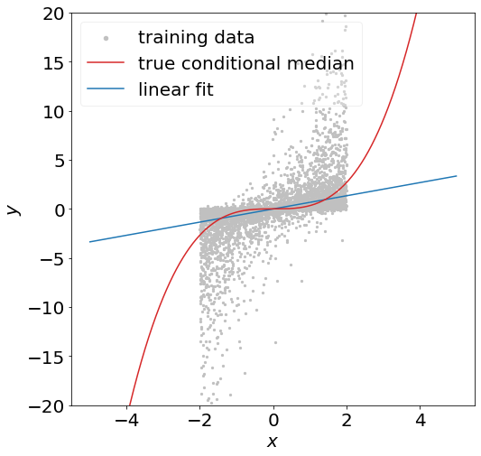
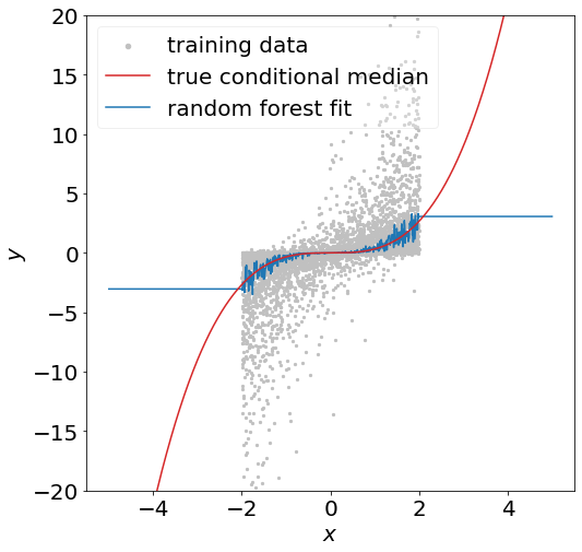
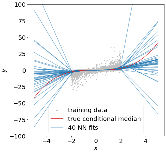
(a) linear model	(b) tree-based model	(c) neural network

Figure 1: Failure examples of nonlinear extrapolation for different model classes. The true (conditional median) function is a cubic function. We use linear quantile regression, quantile regression forest, and quantile regression with a two-layer neural network and 100 hidden neurons to fit the training data supported on $[0,2]$, and evaluate the models on a wider range of test data.

The theoretical understanding of extrapolation for nonlinear models is quite limited. Earlier studies, such as the one by Sugiyama et al., (2007), were predicated on the assumption of a bounded density ratio between the training and test distributions. This assumption implies that the test support is nested within the training support, thus excluding the out-of-support extrapolation scenarios that we aim to address. Christiansen et al., (2021) introduced an extrapolation method that presupposes linearity beyond the support, thus imposing stringent constraints on the function class. More recently, Dong and Ma, (2023) explored extrapolation within the class of additive nonlinear functions. They evaluated the average performance of a model under a newly extended distribution, assuming that the marginals are not substantially shifted. However, they did not study the behaviour of the model at distinct test points beyond the training support, an aspect often referred to as point-wise performance.

Extrapolation is also linked to the extensive body of work on domain adaptation or generalisation, with the primary objective being the development of models that can adapt or generalise effectively to potentially divergent test distributions. Such methods typically depend on the integration of a certain degree of data from the test distribution (Ben-David et al.,, 2006; Ganin and Lempitsky,, 2015; Chen and Bühlmann,, 2021), adjusting the test distribution via covariate shift compensation (Sugiyama et al.,, 2007; Gretton et al.,, 2009), or exploiting specific inherent data structures to train a model that is invariant or robust to distribution shifts (Peters et al.,, 2016; Arjovsky et al.,, 2019; Rothenhäusler et al.,, 2021). However, our work diverges from these methodologies by tackling a more fundamental problem: how a model trained on data within a bounded set can extrapolate to a data point that lies outside the training support. We do not specify the test distribution, nor do we utilise data from the test domain.

1.1 Our contributions

Section 2 depicts the full picture of our proposed method, named ‘engression’ (combining ‘extrapolation’ and ‘nonlinear regression’), which is comprised of two ingredients: a model termed the pre-additive noise model (pre-ANM) and distributional regression. Regarding the modelling choice, we present the pre-ANM as an alternative to the often-used post-additive noise models (post-ANM) to describe the relationship between $X$ and $Y$. While post-additive noise, as a convention, is added to the covariates after applying a nonlinear function, pre-additive noise is added before the nonlinearity. We think that the pre-ANM appears to be a more appealing choice for extrapolation. Regarding the estimation method, distributional regression aims to fit the full conditional distribution of $Y$ given $X=x$ rather than focusing on some specific functional of the distribution, such as the conditional mean in least-squares regression. As an immediate advantage, we can estimate the full conditional distribution for new test data but more relevantly, using distributional regression is also shown to enable extrapolation for pre-ANM models, as the variation of the full conditional distribution contains information about the behaviour of the nonlinear functions of interest outside the training support.

Engression is a generic methodology that can be applied to various regression tasks, including point prediction for the conditional mean and quantiles, constructing prediction intervals, as well as sampling from the conditional distribution.

Section 3 presents the theoretical formulation and guarantees for extrapolation at the population level. We start by introducing the concept of extrapolation uncertainty as a measure of the degree of (dis)agreement between two models beyond the training support. We propose the term ‘extrapability’, which measures the capability of a model to extrapolate. Importantly, we consider extrapability both functionally and distributionally. In this context, the ‘model’ may refer to a function, for instance, the conditional mean of $Y$ given $X=x$, or a distribution, specifically the conditional distribution of $Y$ given $X=x$. While previous studies have focused on functional extrapability, we argue that distributional extrapability is a more desirable notion. It can be achieved with much weaker assumptions about the function class and implies functional extrapability in a suitable sense. As an exercise, we demonstrate the extrapability of the pre-ANMs, suggesting the advantage of pre-ANMs over post-ANMs in extrapolation.

Furthermore, we derive a few simple theoretical results about engression. Specifically, we establish the extrapability of engression under modest conditions of a strictly monotone function class, a feat that cannot be achieved by traditional methods such as least-squares regression and quantile regression. To the best of our knowledge, engression is the first methodology that can verifiably extrapolate beyond the support for nonlinear monotone functions (without the need to assume Lipschitz continuity). We also provide a quantification of the advantage of engression by examining the discrepancies between the extrapolation uncertainty of engression and that of benchmark methods, suggesting that engression consistently delivers an advantage globally. Interestingly, we demonstrate that engression can benefit from a high noise level: larger noise levels actually assist with extrapolation by employing engression. While much of our theoretical analysis is geared toward the univariate case, which already poses a significant challenge to extrapolation, our method can readily handle multivariate predictors and multivariate response variables.

Section 4 is devoted to the finite-sample analysis of the engression estimator. We derive the finite-sample bounds for parameter estimation and prediction for the conditional mean or quantiles, especially outside the support, under specific settings of quadratic models. While traditional regression methods produce arbitrarily large errors outside the support, we show that engression attains consistency for both in-support and out-of-support data. Furthermore, when the pre-additive noise assumption is violated, the model yield by engression defaults to a linear fit that provides a useful baseline performance in comparison to the arbitrarily large extrapolation error from regression. In addition, we show the consistency in terms of estimating the true conditional median function, especially for $x$ outside the support, and the noise distribution for general monotone and Lipschitz functions.

In Section 5, we present comprehensive empirical studies using both simulated data and an assortment of real-world data sets. Our studies cover a range of regression tasks, including univariate and multivariate prediction, as well as prediction intervals. The promising results lend support to our theory and indicate the broad applicability and versatility of the engression method.

1.2 Software

The software implementations of engression are available in both R and Python packages engression with the source code at https://github.com/xwshen51/engression. GPU acceleration is for now only available in the Python version, but CPU-based training, while slower in general, is still suitable for moderately large data sets of up to a few hundred variables and a few thousand observations on a standard single-core machine.

Below is already an example to demonstrate how the software can be used in R (with default options) on a simple linear model, where the test distribution is slightly shifted from the training distribution (a linear least-squares or quantile fit would be clearly be a better choice for this linear model example).

> n = 1000; p=5                                      ## 1000 samples and 5 dimensional covariate
> beta = rnorm(p)                                    ## random regression coefficients
> X = matrix(rnorm(n*p), ncol=p)                     ## design matrix
> Y = X %*% beta + rnorm(n)                          ## linear model
> Xtest = matrix(1 + rnorm(n*p), ncol=p)             ## test data are slightly shifted
> Ytest = Xtest %*% beta + rnorm(n)

> library(engression)                                ## load engression package
> engressionFit = engression(X, Y)                   ## fit an engression model
> yhatEngression = predict(engressionFit, Xtest)     ## predict on test data
> mean((yhatEngression - Ytest)^2)                   ## evaluate conditional mean prediction on test data
[1] 1.045293
> predict(engressionFit, Xtest, type="quantile",     ## quantile prediction with the same engression object
quantiles=c(0.1, 0.5, 0.9))

1.3 Notation

For a univariate function $f(x)$, let $\dot{f}(x)$ be its derivative and $\ddot{f}(x)$ be its second derivative. For $x\in\mathbb{R}$, let $(x)_{+}=\max\{x,0\}$. For a vector $x\in\mathbb{R}^{d}$, let $\|x\|$ be the Euclidean norm. For a random variable $X$ and $\alpha\in[0,1]$, let $Q_{\alpha}(X):=\inf\{x:\mathbb{P}(X\leq x)\geq\alpha\}$ be the $\alpha$-quantile of $X$, or simply denoted by $Q_{\alpha}^{X}$. For random variables $X$ and $X^{\prime}$ that follow the same distribution, we denote by $X\overset{d}{=}X^{\prime}$. For $L>0$, a function $f:\mathbb{R}^{d}\to\mathbb{R}$ is $L$-Lipschitz continuous if $|f(x)-f(x^{\prime})|\leq L\|x-x^{\prime}\|$ for all $x,x^{\prime}\in\mathbb{R}^{d}$. Throughout the paper, all distributions are assumed to be absolutely continuous with respect to the Lebesgue measure unless stated otherwise.

2 Engression

In Section 2.1, we discuss the pre- and post-additive noise as different ways to model the nonlinear relationship between $X$ and $Y$. In Section 2.2, we discuss distributional regression and non-distributional regression. In Section 2.3, we propose the engression method, which entails distributional regression for pre-additive noise models.

2.1 Pre-Additive versus Post-Additive Noise Models

Conventionally, a regression model assumes that noise is added after applying a nonlinear transformation to the covariates $X$,

$$Y=g(WX)+\eta,$$ (1)

a model we refer to as the post-additive noise model (post-ANM), where $W\in\mathbb{R}^{k\times d}$, $g:\mathbb{R}^{k}\to\mathbb{R}$ is a nonlinear function, and $\eta$ is a random variable with an unknown distribution representing the noise. Taking $W$ to be the identity matrix, the model becomes $Y=g(X)+\eta$ which is the standard form in nonlinear regression. When $k=1$, the model is a single index model (McCullagh and Nelder,, 1983; Hardle et al.,, 1993; Brillinger,, 2012).

Contrarily, we propose the pre-additive noise model (pre-ANM), wherein the noise is added directly to $X$ prior to any nonlinear transformation, represented as

$$Y=g(WX+\eta)+\beta^{\top}X,$$ (2)

where $\beta\in\mathbb{R}^{d}$, and the noise $\eta$ is a random vector unless we take $k=1$. Note that the linear term $\beta^{\top}X$ is merely for adding more flexibility to the model but not necessary for extrapolation, and it can be dropped by setting $\beta=0$.

This seemingly minor difference in the position of the noise can significantly impact the extrapability of the model. Intuitively, the response variable generated according to a post-ANM is a vertically perturbed version of the true function, whereas the response from a pre-ANM is a horizontally perturbed version. As such, if the data are generated according to a post-ANM, the observations for the response variable are perturbed values of the true function evaluated at covariate values within the support. We hence generally have no data-driven information about the behaviour of the true function outside the support. In contrast, data generated from a pre-ANM contain response values that reveal some information beyond the support.

In fact, we will establish in Section 3.2 that pre-ANMs are extrapable under mild assumptions, specifically when $g$ is strictly monotone, whereas post-ANMs fail to be extrapable unless one imposes stringent assumptions on $g$, such as belonging to a linear function class. Furthermore, in subsequent sections, we demonstrate that the pre-additive noise can be beneficial for extrapolation: larger noise levels actually assist with extrapolation, thus transforming what could be a curse into a blessing, given that we use distributional regression.

2.1.1 Connections to existing modelling approaches

It is important to note that pre-ANMs bear certain resemblances to the post-nonlinear models featured in literature. In the context of nonlinear independent component analysis, given an independent source vector $S$, the post-nonlinear mixture (Taleb and Jutten,, 1999) hypothesises that the observed mixture $X$ is formed through component-wise nonlinearities applied to the components of the linear mixture, represented as:

$$X_{i}=g_{i}([WS]_{i}),$$

where $i=1,\dots,d$, $W$ is a linear transformation, and $g$ is a component-wise invertible nonlinear function. However, in contrast to our context, this is a deterministic process with the distinct aim of recovering the hidden signal $S$ from $X$.

In causality, Zhang and Hyvärinen, (2009) extended the post-nonlinear mixture to the post-nonlinear causal model, which models the causal relationship between a variable $Y$ and its direct cause $X$ as:

$$Y=g_{2}(g_{1}(X)+\varepsilon),$$

where $g_{1}$ denotes the nonlinear causal effect, $g_{2}$ the invertible post-nonlinear distortion in $Y$, and $\varepsilon$ the independent noise. The crucial difference between this model and the pre-ANM is whether the noise $\varepsilon$ is directly added to $X$, up to a linear transformation. This attribute forms the cornerstone of pre-ANMs, which is not the case for post-nonlinear models unless $g_{1}$ is linear. Besides, the pre-ANM allows for additional linear terms that do not show up in a post-nonlinear model.

Furthermore, assuming $g$ is invertible, the pre-ANM in (2) without the linear term can be written as $g^{-1}(Y)=WX+\eta$, which appears to be a linear model after transforming $Y$. Invertibility of $g$ requires that $k$ is equal to the dimension of the response. In many applications, it is common to transform the response variable by a pre-defined function, such as logarithm, based on domain expertise. This indicates from a practical perspective that the pre-ANMs could potentially fit many real data well. However, manually choosing the suitable transformation becomes inplausible especially when we have multivariate variables $Y$ and $X$. Moreover, with an additional linear term, the pre-ANM can no longer be captured through such a transformation. Thus, our proposed method goes even beyond learning the suitable transformation of $Y$ in a data-driven way.

2.2 Distributional regression versus non-distributional regression

Regression is a well-established technique for estimating the dependence of the response variable $Y$ given the covariates $X$. The most classical view of regression focuses on estimating the conditional mean of $Y$ given $X=x$, with the most prevalent technique being the least-squares regression, also known as $L_{2}$ regression (Legendre,, 1806). Specifically, it searches among a function class $\mathcal{F}$ for the best fit that minimises the $L_{2}$ risk, i.e.

$$\min_{f\in\mathcal{F}}\mathbb{E}[(Y-f(X))^{2}].$$ (3)

Beyond the conditional mean, other functionals of the conditional distribution have been considered, such as quantiles. Given $\alpha\in[0,1]$, quantile regression (Koenker,, 2005) is defined as the solution to

$$\min_{f\in\mathcal{F}}\mathbb{E}[\rho_{\alpha}(Y-f(X))],$$ (4)

where $\rho_{\alpha}(x):=x(\alpha-\mathbf{1}_{(x<0)})$. In the special case with $\alpha=0.5$, quantile regression becomes the least absolute deviation regression, also known as $L_{1}$ regression, i.e.

$$\min_{f\in\mathcal{F}}\mathbb{E}|Y-f(X)|,$$ (5)

which is used for estimating the conditional median of $Y$ given $X=x$.

In all the aforementioned techniques, the conditional distribution is summarised in a univariate quantity of interests, which may often lead to the most efficient approach in terms of the in-support performance. However, when it comes to extrapolation outside the support, even with the same goal of point prediction, one should aim for more than just the quantity of interest, but should instead fit the entire distribution. For example, the out-of-support information revealed by a pre-ANM requires a full capture of the noise distribution, which is essentially the conditional distribution of $Y$ given $X=x$. This intuition, along with more formal arguments in Section 3.1, suggests to estimate the full conditional distribution of $Y$ given $X=x$, which aligns with the aim of distributional regression.

Both parametric and non-parametric approaches have been developed for distributional regression through estimating the cumulative distribution function (Foresi and Peracchi,, 1995; Hothorn et al.,, 2014), density function (Dunson et al.,, 2007), quantile function (Meinshausen,, 2006), etc. See a recent review of distributional regression approaches in Kneib et al., (2023).

Another perspective that emerges more dramatically in machine learning is (conditional) generative modelling (Goodfellow et al.,, 2014; Mirza and Osindero,, 2014). Therein, the goal is to learn a random function $G$ of $x$ such that the distribution of $G(X)$ given $X=x$ is identical to the true conditional distribution of $Y$ given $X=x$, which is often approached by minimising a certain statistical distance such as the Kullback–Leibler (KL) divergence. As a result, generative modelling also fits the full conditional distribution. However, instead of estimating the conditional distribution function, such as the density, a generative model enables sampling from the conditional distribution.

It is worth pointing out that distributional regression approaches provide estimation for the conditional distribution which in principle can be used to estimate any functionals of the distribution, such as the conditional mean. This is particularly easy based on a generative model, since it enables estimation through sampling. Therefore, even when the primary objective of data analysis is point prediction, distributional regression is still a valid approach. More importantly, as we will show later, a distributional regression approach can result in better performance in terms of extrapolation of, for example, the conditional mean than a regression approach that is designed to model the conditional mean directly.

2.2.1 Assessing distributional regression

We give a brief introduction on quantitative ways to assess a distributional fit. The energy score introduced by Gneiting and Raftery, (2007) is a popular scoring rule for evaluating multivariate distributional predictions. For a random vector $Z$ that follows a distribution $P$ and an observation $z$, the energy score is defined as

$$\mathrm{ES}(P,z)=\frac{1}{2}\mathbb{E}_{P}\|Z-Z^{\prime}\|-\mathbb{E}_{P}\|Z-z\|,$$ (6)

where $Z$ and $Z^{\prime}$ are two independent draws from $P$. Note that the higher the score, the better the distributional prediction. We will generally use the negative of the energy score to design a loss function and call it energy loss where appropriate. The following lemma based on the results in Székely, (2003) and Székely and Rizzo, (2023) states that the energy score is a strictly proper scoring rule.

Lemma 1.

For any distribution $P^{\prime}$, we have $\mathbb{E}_{Z\sim P}[\mathrm{ES}(P,Z)]\geq\mathbb{E}_{Z\sim P^{\prime}}[\mathrm{ES}(P,Z)]$, where the equality holds if and only if $P$ and $P^{\prime}$ are identical.

When $Z$ is univariate whose cumulative distribution function (cdf) is denoted by $F$, the energy score reduces to the continuous ranked probability score (CRPS) (Matheson and Winkler,, 1976) defined as

$$\mathrm{CRPS}(F,z)=-\int_{-\infty}^{\infty}(F(z^{\prime})-\mathbf{1}\{z^{\prime}\geq z\})^{2}dz^{\prime}.$$

The equality between CRPS and the energy score in (6) in the univariate case was shown by Baringhaus and Franz, (2004), which is essentially a distributional extension of the (negative) absolute error.

These scoring rules are associated with certain distance functions. In particular, the respective distance of the energy score for two distributions $P$ and $P^{\prime}$ is the energy distance (Székely,, 2003) defined as

$$\mathrm{ED}(P,P^{\prime})=2\mathbb{E}\|Z-Z^{\prime}\|-\mathbb{E}\|Z-\tilde{Z}\|-\mathbb{E}\|Z^{\prime}-\tilde{Z}^{\prime}\|,$$ (7)

where $Z$ and $\tilde{Z}$ are two independent draws from $P$, and $Z^{\prime}$ and $\tilde{Z}^{\prime}$ are independent draws from $P^{\prime}$. The distance associated with CRPS for two cdf’s $F$ and $F^{\prime}$ is the Cramér distance (Székely,, 2003) defined as

$$\mathrm{CD}(F,F^{\prime})=\int_{-\infty}^{\infty}(F(z)-F^{\prime}(z))^{2}dz.$$

Both the energy distance and the Cramér distance are special cases of the maximum mean discrepancy (MMD) distance (Gretton et al.,, 2012; Sejdinovic et al.,, 2013) and had been incorporated in Bellemare et al., (2017) in the context of generative adversarial networks (Goodfellow et al.,, 2014). Along the same line, other distances or divergences have been adopted, such as the Wasserstein distance (Arjovsky et al.,, 2017; Gulrajani et al.,, 2017) or $f$-divergence (Nowozin et al.,, 2016; Shen et al.,, 2022).

2.3 Engression methodology

The previous sections showed the two main ingredients of engression, namely

1. distributional regression in conjunction with

2. a pre-additive noise model (pre-ANM).

In fact, both ingredients are necessary for reliable extrapolation. We later provide some evidence of successful extrapolation for engression. In contrast, results in Section 3.2 indicate the failure of distributional regression in conjunction with post-ANMs, while results in Section 3.3 show the failure of the combinations of non-distributional approaches with pre- or post-ANMs.

Based on the proposed pre-ANM in (2), we define the pre-ANM class as

$$\mathcal{M}_{\mathrm{pre}}=\{\textsl{g}(x,\varepsilon):=g(W^{\top}x+h(\varepsilon))+\beta^{\top}x:W\in\mathbb{R}^{k\times d},\beta\in\mathbb{R}^{d},g\in\mathcal{G},h\in\mathcal{H}\},$$

where $\mathcal{G}$ and $\mathcal{H}$ are two function classes, and $\varepsilon$ is a random vector with a pre-specified distribution, e.g. a multivariate uniform distribution with independent components. Herein, each model is represented by a function g that takes two arguments: covariates $x$ and noise $\varepsilon$, and depends on a tuple $(W,\beta,g,h)$. Note that each model in $\mathcal{M}_{\mathrm{pre}}$ induces a conditional distribution of $Y$ given $X=x$. Specifically, for $\textsl{g}\in\mathcal{M}_{\mathrm{pre}}$ and $x\in\mathbb{R}^{d}$, denote by $P_{\textsl{g}}(y|x)$ the conditional distribution of $\textsl{g}(X,\varepsilon)$ given $X=x$.

We define the solution $\tilde{\textsl{g}}$ to the population version of engression as

$$\tilde{\textsl{g}}\in\operatorname*{argmin}_{\textsl{g}\in\mathcal{M}_{\mathrm{pre}}}\mathbb{E}_{X\sim P_{\mathrm{tr}}(x)}[\mathcal{L}(P_{\textsl{g}}(y|X);P_{\mathrm{tr}}(y|X))],$$ (8)

where $\mathcal{L}(P;P_{0})$ is a loss function for a distribution $P$ given a reference distribution $P_{0}$. We will define the finite-sample version of engression after specifying the choice for the loss function.

Engression allows a rather flexible choice of the loss function, with the only requirement being the characterisation property: for all distribution $P$, it holds that $\mathcal{L}(P;P_{0})\geq\mathcal{L}(P_{0};P_{0})$, where the equality holds if and only if $P=P_{0}$. It can be designed based on a statistical distance. Note that when the function classes $\mathcal{G}$ and $\mathcal{H}$ are nonparametric classes or neural networks, the loss function based on the KL divergence or Wasserstein distance in general does not have an analytic form to be easily optimised. For such loss functions, one typical solution is to adapt the generative adversarial networks (Goodfellow et al.,, 2014), which is more computationally involved.

In comparison, the energy score (6) or energy distance (7) are appealing due to their computational simplicity: the estimation of the score or distance is based on sampling. This works nicely with the generative nature of the pre-ANM. Specifically, for any given $x$, one can sample from the conditional distribution $P_{\textsl{g}}(y|x)$ by first sampling the random vector $\varepsilon\sim\mathrm{Unif}[0,1]$ and then applying the transformation based on the pre-ANM to obtain a sample. Therefore, in this work, our primary choice for the loss function is the energy loss based on the negative energy score, defined as

$$\mathcal{L}_{e}(P;P_{0}):=\mathbb{E}_{Y\sim P_{0}}[-\mathrm{ES}(P,Y)].$$

Then the objective function in engression (8) yields

$$\begin{split}&\mathbb{E}_{X\sim P_{\mathrm{tr}}(x)}[\mathcal{L}_{e}(P_{\textsl{g}}(y|X);P_{\mathrm{tr}}(y|X))]\\ =\ &\mathbb{E}_{X\sim P_{\mathrm{tr}}(x)}\Big{[}\mathbb{E}_{Y\sim P_{\mathrm{tr}}(y|X),\varepsilon}|Y-\textsl{g}(X,\varepsilon)|-\frac{1}{2}\mathbb{E}_{\varepsilon,\varepsilon^{\prime}}|\textsl{g}(X,\varepsilon)-\textsl{g}(X,\varepsilon^{\prime})|\Big{]},\end{split}$$ (9)

where $\varepsilon$ and $\varepsilon^{\prime}$ are independent draws from $\mathrm{Unif}[0,1]$. This form facilitates the computation and estimation based on a finite sample.

Nevertheless, it is worth pointing out that all of our theoretical results in Section 3 hold for any loss functions that satisfy the above characterisation property. We investigate the empirical performance of engression with other loss functions in Appendix D including the MMD distance and KL divergence, where we observe that different loss functions result in comparable performance. While it will be worthwhile to discuss the relative advantages from a theoretical point of view, we work primarily with the energy loss because it is simple to understand without the need to choose further hyperparameters, is computationally fast as it does not require adversarial training, and is empirically well behaved during optimisation.

2.3.1 Finite-sample engression

Consider an i.i.d. sample $\{(X_{i},Y_{i}):i=1,\dots,n\}$ from $P_{\mathrm{tr}}(x,y)$. For each observation, we sample the noise variable $\varepsilon$ independently from $\mathrm{Unif}[0,1]$ for $m$ times, resulting in an i.i.d. sample $\{\varepsilon_{i,j}:i=1,\dots,n,j=1,\dots,m\}$. Based on the finite samples, we define the empirical version of engression as

$$\hat{\textsl{g}}\in\operatorname*{argmin}_{\textsl{g}\in\mathcal{M}_{\mathrm{pre}}}\hat{\mathcal{L}}(\textsl{g})$$ (10)

with the empirical objective function given by

$$\hat{\mathcal{L}}(\textsl{g}):=\frac{1}{n}\sum_{i=1}^{n}\left[\frac{1}{m}\sum_{j=1}^{m}|Y_{i}-\textsl{g}(X_{i},\varepsilon_{i,j})|-\frac{1}{2m(m-1)}\sum_{j=1}^{m}\sum_{j^{\prime}=1}^{m}|\textsl{g}(X_{i},\varepsilon_{i,j})-\textsl{g}(X_{i},\varepsilon_{i,j^{\prime}})|\right],$$

which is an unbiased estimator of the population objective function (9). We parameterise the pre-ANMs using neural networks. Then the above empirical objective function is differentiable with respect to all the model parameters. Thus, we adopt (stochastic) gradient descent algorithms (Cauchy,, 1847; Robbins and Monro,, 1951) to solve the optimisation problem in (10).

2.3.2 Point prediction

Engression, being a distributional regression method, estimates the conditional distribution of $Y$ given $X=x$, thus also providing estimators for various characteristics of the distribution such as the mean and quantiles. Specifically, at the population level, the engression estimator for the conditional mean of $Y$ given $X=x$ is derived from $\tilde{\mu}(x):=\mathbb{E}_{\varepsilon}[\tilde{\textsl{g}}(x,\varepsilon)]$. The engression estimator for the conditional median is $\tilde{m}(x):=Q_{0.5}(\tilde{\textsl{g}}(x,\varepsilon))$, where the quantile is taken with respect to $\varepsilon$. For any $\alpha\in[0,1]$, the engression estimator for the conditional $\alpha$-quantile is $\tilde{q}_{\alpha}(x):=Q_{\alpha}(\tilde{\textsl{g}}(x,\varepsilon))$.

For a finite sample, based on the empirical engression solution $\hat{\textsl{g}}$, we construct the estimators by sampling. Specifically, for any $x$, we sample $\varepsilon_{i},i=1,\dots,m$ for some $m\in\mathbb{N}_{+}$, and then obtain $\hat{\textsl{g}}(x,\varepsilon_{i}),i=1,\dots,m$. These form an i.i.d. sample from the conditional distribution $p_{\hat{\textsl{g}}}(y|x)$. All the quantities are then estimated using their empirical versions from this sample. For instance, the conditional mean of $Y$ given $X=x$ is estimated by $\frac{1}{m}\sum_{i=1}^{m}\hat{\textsl{g}}(x,\varepsilon_{i})$.

2.3.3 Air quality data example

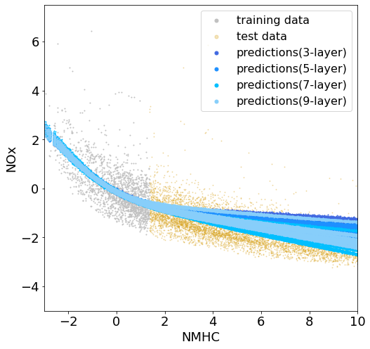
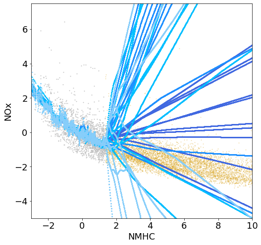
(a) Engression	(b) Regression

Figure 2: Out-of-support predictions by engression and $L_{2}$ regression on the air quality data. The models are trained on a support up to the first quartile of NMHC and evaluated in their predictions for larger NMHC values. To ensure a fair comparison, we apply both methods with the same neural network architecture whose number of layers is varying from 3 to 9; for each architecture, we repeatedly employ both methods for ten times (each with an independent random initialisation) and show the behaviour of all of them.

Before presenting the formal theory, we demonstrate engression versus regression using the air quality data set from Vito, (2016), where we take the measurements of two pollutants, NMHC and NOx, as the predictor and response variables, respectively. We partition the data into training and test sets at the first quartile of the predictor and take the smaller portion for training. As visualised in Figure 2, engression and regression work comparably well within the training data while behaving very differently on out-of-support test data, despite the same underlying network architectures being used. Engression maintains excellent prediction performance on test data beyond the training boundary up to a certain range, when it starts to diverge moderately. In contrast, regression produces highly variable predictions that spread out the whole space once going outside the support. Especially as the number of layers in the neural network grows, the out-of-support predictions by regression disperse even wider, whereas engression is highly robust to various model architectures.

In the sequel, we delve deeper into theoretical and empirical perspectives of engression. Section 3 presents the formal theory of extrapolation and justify the virtue of engression in this regard. Section 4 provides finite-sample guarantees for the engression estimator. Section 5 is devoted to large-scale experimental investigations.

3 Theory of extrapolation

In Section 3.1, we define extrapolation uncertainty and extrapability for a given model class. As a demonstration, in Section 3.2, we study the extrapability of pre-ANMs and post-ANMs. Section 3.3 discusses the extrapability of engression, while Section 3.4 quantifies the extrapability gains of engression compared to the baseline methods. All results in this section are at the population level.

3.1 Extrapability

In this section, we define extrapability through the notions of extrapolation uncertainty at functional and distributional levels. The term ‘uncertainty’ here refers to the spread among out-of-support predictions that arises due to partially observing the sample space and the fact that multiple functions or models fit the in-support data equally well, as made more precise further below. It is in particular distinct from the ‘stochastic uncertainty’ caused by the randomness from a finite sample.

We start with the extrapolation uncertainty and extrapability in terms of a function class which includes the notion of extrapolation used in existing literature as a special case. For any $x\in\mathbb{R}^{d}$, define the distance between $x$ and set $\mathcal{X}$ by $d(x,\mathcal{X})=\inf_{x^{\prime}\in\mathcal{X}}\|x-x^{\prime}\|$.

Definition 1 (Functional extrapability).

Let $\mathcal{F}$ be a function class of $x\in\mathbb{R}^{d}$. For $\delta>0$, define the functional extrapolation uncertainty of a function class $\mathcal{F}$ as

$$\mathcal{U}_{\mathcal{F}}(\delta):=\sup_{x^{\prime}:d(x^{\prime},\mathcal{X})\leq\delta}\sup_{\begin{subarray}{c}f,f^{\prime}\in\mathcal{F}:\\ D_{x}(f,f^{\prime})=0,\forall x\in\mathcal{X}\end{subarray}}D_{x^{\prime}}(f,f^{\prime}),$$

where $D_{x}(f,f^{\prime}):=|f(x)-f^{\prime}(x)|$ for all $x\in\mathbb{R}^{d}$. $\mathcal{F}$ is said to be (globally) functionally extrapable, if $\mathcal{U}_{\mathcal{F}}(\delta)\equiv 0$.

In words, the functional extrapolation uncertainty quantifies the worst-case disagreement of two functions that agree perfectly within the support. The following examples illustrate the functional extrapolation uncertainty of several common function classes, which are proved in Appendix A.1.

Example 1 (Linear functions).

Linear functions are functionally extrapable, i.e. $\mathcal{U}(\delta)\equiv 0$. Note that the functional extrapability has appeared in existing work, e.g. Christiansen et al., (2021). It essentially requires the function to be uniquely determined by its values on the support.

Example 2 (Lipschitz functions).

The functional extrapolation uncertainty of the class of $L$-Lipschitz continuous functions is $\mathcal{U}(\delta)=2L\delta$.

Example 3 (Monotone functions).

The functional extrapolation uncertainty of a class of (component-wise) monotone functions is $\mathcal{U}(\delta)=\infty$.

In the context of prediction, the relationship between $X$ and $Y$ is comprehensively captured by the conditional distribution of $Y$ given $X=x$. Consider a class $\mathcal{P}=\{P(y|x)\}$ of conditional distributions. Standard prediction tasks are often concerned with a certain characteristic quantity, such as the conditional mean function $\mu_{P}(x)=\mathbb{E}_{P(y|x)}[Y]$ or conditional quantile functions. Taking the conditional mean as an example, we define below the mean extrapability which is a direct extension of the functional extrapability towards a distributional level.

Definition 2 (Mean extrapability).

For $\delta>0$, define the mean extrapolation uncertainty of $\mathcal{P}$ as

$$\mathcal{U}^{\mu}_{\mathcal{P}}(\delta):=\sup_{x^{\prime}:d(x^{\prime},\mathcal{X})\leq\delta}\sup_{\begin{subarray}{c}P,P^{\prime}\in\mathcal{P}:\\ D_{x}(P,P^{\prime})=0,\forall x\in\mathcal{X}\end{subarray}}D_{x^{\prime}}(P,P^{\prime}),$$

where $D_{x}(P,P^{\prime}):=|\mu_{P}(x)-\mu_{P^{\prime}}(x)|$ for all $x\in\mathbb{R}^{d}$.

In Definition 2, the distance between two distributions is measured by the difference between the two conditional means. A more general way instead is to use a statistical distance, denoted by $D(P,P^{\prime})$, between two probability distributions $P$ and $P^{\prime}$, such as the Wasserstein distance or KL divergence. This leads us to the final notion of extrapability in terms of a class of distributions.

Definition 3 (Distributional extrapability).

For $\delta>0$, define the distributional extrapolation uncertainty of $\mathcal{P}$ as

$$\mathcal{U}_{\mathcal{P}}(\delta):=\sup_{x^{\prime}:d(x^{\prime},\mathcal{X})\leq\delta}\sup_{\begin{subarray}{c}P,P^{\prime}\in\mathcal{P}:\\ D_{x}(P,P^{\prime})=0,\forall x\in\mathcal{X}\end{subarray}}D_{x^{\prime}}(P,P^{\prime}),$$

where $D_{x}(P,P^{\prime}):=D(P(y|x),P^{\prime}(y|x))$ for all $x\in\mathbb{R}^{d}$. $\mathcal{P}$ is said to be (globally) distributionally extrapable, if $\mathcal{U}_{\mathcal{P}}(\delta)\equiv 0$.

The distributional extrapolation uncertainty provides an upper bound on the degree of disparity between two conditional distributions outside the support, given that they coincide within the support. Distributional extrapability implies that the conditional distribution of $Y$ given $X=x$ for all $x$ globally is uniquely determined by the conditional distributions of $Y$ given $X=x$ for all $x$ within the support.

Perhaps surprisingly, unlike functional extrapability, which imposes stringent constraints on the function class (such as linearity, as discussed in Example 1), distributional extrapability can be achieved under relatively mild conditions. These will be realised concretely in Theorem 1 below.

We conclude this section by illuminating the connections among the three levels of extrapability. In essence, mean extrapability serves as a bridge between functional and distributional extrapability, shedding light on how the latter concept can ‘imply’ the former in a specific sense. The key insight here is that when two conditional distributions $P(y|x)$ and $P^{\prime}(y|x)$ are in agreement within the support, their corresponding conditional mean functions also coincide within this same support. If distributional extrapability holds, which secures the agreement of $P(y|x)$ and $P^{\prime}(y|x)$ outside the support, then their conditional means will likewise align outside the support. Conversely, if we only have the knowledge that the conditional means of $P(y|x)$ and $P^{\prime}(y|x)$ are the same within the support, full distributional agreement is, however, not guaranteed. Therefore, for the conditional means to be consistent beyond the support, the prerequisite is the functional extrapability of the class of conditional mean functions.

This insight implies that if a method is solely aimed at fitting the conditional mean function, its ability to extrapolate beyond the training support relies fully on the extrapability of the function class itself, which could be highly restrictive. In contrast, a method that aims to match the entire conditional distribution needs potentially much weaker assumptions on the function class for successful extrapolation. This suggests from another perspective than the intuitions provided in Section 2.2 that distributional regression could bring in more potential for extrapolation.

3.2 Extrapability of ANMs

For ease of presentation, starting from this section, we will primarily focus on the univariate case with $X\in\mathbb{R}$ unless stated otherwise. We introduce some additional notation. In the univariate case, the post-ANM is expressed as $Y=g(X)+\eta,$ where $g$ is a univariate nonlinear function and the parameter $W$ in (1) is absorbed into $g$. We assume $\eta$ is independent from $X$ and follows an arbitrary distribution that is absolutely continuous with respect to the Lebesgue measure so that $\eta\overset{d}{=}h^{\star}(\varepsilon)$ for a strictly monotone function $h^{\star}$ and a random variable $\varepsilon\sim\mathrm{Unif}[0,1]$. Note that $\varepsilon$ can in principle be any continuous random variable and we choose the uniform distribution for convenience. Also assume without loss of generality that $\eta$ has a zero median so that $h^{\star}(0.5)=0$, which avoids trivial non-identifiability. Define function classes $\mathcal{G}=\{g(x)\}$ and $\mathcal{H}=\{h(\varepsilon):h(0.5)=0,h\text{ is strictly monotone}\}$. We denote by $\mathcal{M}_{\mathrm{post}}=\{g(x)+h(\varepsilon):g\in\mathcal{G},h\in\mathcal{H}\}$ a class of post-ANMs. Similarly, the pre-ANM is of the following form

$$Y=g(X+\eta)+\beta X.$$ (11)

We denote by $\mathcal{M}_{\mathrm{pre}}=\{g(x+h(\varepsilon))+\beta x:g\in\mathcal{G},h\in\mathcal{H},\beta\in\mathbb{R}\}$ a class of pre-ANMs.

Note that any model in $\mathcal{M}_{\mathrm{pre}}$ or $\mathcal{M}_{\mathrm{post}}$ induces a conditional distribution of $Y$, given $X=x$. For example, a post-ANM $g(X)+\eta$ with $\eta\sim\mathcal{N}(0,1)$ follows a Gaussian distribution $\mathcal{N}(g(x),1)$ conditional on $X=x$. Thus, the extrapability of $\mathcal{M}_{\mathrm{pre}}$ or $\mathcal{M}_{\mathrm{post}}$ is defined as the distributional extrapability of the class of conditional distributions induced by the models in $\mathcal{M}_{\mathrm{pre}}$ or $\mathcal{M}_{\mathrm{post}}$.

Definition 4 (Linear and nonlinear pre-ANMs).

A pre-ANM class $\mathcal{M}_{\mathrm{pre}}$ is said to be linear if $\mathcal{G}$ belongs to a linear function class. A pre-ANM class $\mathcal{M}_{\mathrm{pre}}$ is said to be nonlinear if for all $g\in\mathcal{G}$, for all $h\in\mathcal{H}$ and $\varepsilon\in[0,1]$, it holds that $g$ is twice differentiable and there exists $x\in\mathcal{X}$ such that $\ddot{g}(x+h(\varepsilon))\neq 0$.

The following theorem formalises the extrapability of a pre-ANM class, either linear or nonlinear, in contrast to the non-extrapability of a post-ANM class.

Theorem 1.

Assume $h$ is unbounded for all $h\in\mathcal{H}$, i.e. for any $B>0$, there exists $\varepsilon_{1},\varepsilon_{2}$, such that $h(\varepsilon_{1})>B$ and $h(\varepsilon_{2})<-B$. If $g$ is strictly monotone and twice differentiable for all $g\in\mathcal{G}$, then we have

1. both linear and nonlinear $\mathcal{M}_{\mathrm{pre}}$ are distributionally extrapable, i.e. $\mathcal{U}_{\mathrm{pre}}(\delta)=0$;

2. $\mathcal{M}_{\mathrm{post}}$ has infinite distributional extrapolation uncertainty, i.e. $\mathcal{U}_{\mathrm{post}}(\delta)=\infty$.

In fact, $\mathcal{G}$ being functionally extrapable is the sufficient and necessary condition for $\mathcal{M}_{\mathrm{post}}$ to be distributionally extrapable.

The proof is provided in Appendix A.2. The assumptions for a pre-ANM class to perform extrapolation include the unboundedness of $h$ and the monotonicity of the function class $\mathcal{G}$. The first assumption essentially asserts that the noise $\eta=h(\varepsilon)$ is supported on $\mathbb{R}$, meaning that it has a strictly positive density on $\mathbb{R}$. While this may seem like a mild assumption, in transitioning from a population case to finite samples, we must acknowledge that the empirical support of the training data is always finite. Thus, starting from the next section, we will navigate towards a more realistic scenario where the noise $\eta$ may have a bounded support. The assumption of monotonicity is also much broader than assuming the functional extrapability of the function class. Nevertheless, we can relax the requirement for global monotonicity to that of monotonicity only in proximity to the boundary of the support.

Theorem 1 highlights the substantial advantage that pre-ANMs have in extrapolation: under identical (and mild) assumptions, pre-ANMs satisfy distributional extrapability, whereas post-ANMs fail to extrapolate unless the function class is inherently extrapable. This verifies the intuitions provided in Section 2.1 on why pre-ANMs could offer more potential for extrapolation than post-ANMs. Note that although a linear pre-ANM class is not identifiable (i.e. there exist two linear pre-ANMs that induce the same conditional distribution of $Y|X$), it still satisfies the distributional extrapability according to Theorem 1. In fact, the two model classes $\mathcal{M}_{\mathrm{pre}}$ and $\mathcal{M}_{\mathrm{post}}$ only coincide when $\mathcal{G}$ is a linear function class, which is in harmony with the functional extrapability of linear functions presented in Example 1.

It is worth noting that one could establish extrapability for a model that allows for both pre- and post-additive noises, for example, as follows

$$Y=g(X+\eta)+\beta X+\xi,$$

where $\eta$ is the pre-additive noise while $\xi$ is the post-additive noise. In Appendix C, we provide an example of this possibility while more general investigations are worthwhile in future research.

3.3 Extrapability of engression

Next, we take a closer look at the extrapability properties and guarantees of engression. Denote the solution to the population engression in (8) explicitly by $(\tilde{g},\tilde{h},\tilde{\beta})$. Based on the definitions in Section 3.1, we define the extrapability of a method as the extrapability of the class of estimators obtained from that method. For a quantity q of interest, denote by $\mathcal{F}^{\textsl{q}}_{\mathrm{E}}$ the class of functions for estimating the quantity q obtained by applying engression on the training distribution. Specifically, we use $\textsl{q}=\textsl{m},\mu$ and $\alpha$ to stand for the (conditional) median, mean, and $\alpha$-quantile, respectively. For a method M, denote by $\mathcal{F}_{\textsl{M}}$ the class of functions obtained by applying the method M on the training distribution. Specifically, we use $\textsl{M}=\mathrm{QR},L_{1}$ and $L_{2}$ to represent quantile regression, $L_{1}$ regression, and $L_{2}$ regression, respectively. We denote by $\mathcal{F}^{\alpha}_{\mathrm{QR}}$ the solution set of quantile regression for the $\alpha$-quantile.

Throughout this section, we assume the following conditions are fulfilled.

1. The noise $\eta$ follows a symmetric distribution with a bounded support, i.e. $\eta\in[-\eta_{\max},\eta_{\max}]$ for $\eta_{\max}>0$.

2. The training support is a half line $\mathcal{X}=(-\infty,x_{\max}]$.

3. $g$ is strictly monotone and twice differentiable for all $g\in\mathcal{G}$.

4. The true model, denoted by $Y=g^{\star}(X+h^{\star}(\varepsilon))+\beta^{\star}X$, satisfies $g^{\star}\in\mathcal{G}$, $h^{\star}\in\mathcal{H}$, and $g^{\star}$ is nonlinear, i.e. $\ddot{g}^{\star}(x)\neq 0$ apart from a set with Lebesgue measure 0.

Condition (A1) is not a necessary assumption as a bounded support makes the problem more challenging for extrapolation, as suggested by Theorem 1. We include this assumption to make the setting more plausible for a broader range of real-world scenarios, compared to the requirement of unbounded noise.

Condition (A2) simplifies the discussions by restricting the focus on extrapolation where $x>x_{\max}$. Though this is a technical assumption for ease of analysis, the insights can be extended to scenarios where extrapolation is required on both ends of the support.

Condition (A3) requires the monotonicity and differentiability of the function $g$. Compared to a Lipschitz condition, this assumption presents a tougher challenge for extrapolation. However, it could be readily relaxed to the condition where $g$ is strictly monotone only in the interval $[x_{\max}-\eta_{\max},x_{\max}+\eta_{\max}]$, under which the results regarding the extrapolation for $x$ outside the support would still hold.

Finally, Condition (A4) ensures the correct specification of the model, meaning that the true data generating process $g^{\star}(X+h^{\star}(\varepsilon))+\beta^{\star}X$ belongs to the pre-ANM class $\mathcal{M}_{\mathrm{pre}}$. This condition helps us concentrate our analysis on the extrapolation behaviour of the method, by excluding the effects of any approximation errors. The additional requirement that $g^{\star}$ be nonlinear excludes the linear setting where extrapolation is straightforward and positions us in the pivotal scenario of nonlinear extrapolation.

Given that the noise is bounded, we cannot expect extrapability across the whole real line. However, we can achieve extrapability within a specific range that extends beyond the support, an advantage that is not seen in alternative methods under the same mild conditions. Moreover, in the upcoming subsection, we will compare our method with baseline approaches by quantifying the gains between their extrapolation uncertainty globally on $\mathbb{R}$, where engression constantly holds an advantage.

The following proposition suggests that engression can consistently recover the true function $g^{\star}$ up to a certain range depending on the noise level. This brings up an interesting point that the (pre-additive) noise is a blessing rather than a curse for extrapolation: the more noise one has (i.e. a larger $\eta_{\max}$), the farther one can extrapolate. In fact, this further echoes the result in Theorem 1 which states that with an unbounded noise ($\eta_{\max}\to\infty$), we can achieve global extrapability and recover $g^{\star}$ over the entire real line. The proof is given in Appendix A.3.

Proposition 1.

We have $\tilde{\beta}=\beta^{\star}$, $\tilde{g}(x)=g^{\star}(x)$ for all $x\leq x_{\max}+\eta_{\max}$, and $\tilde{h}(\varepsilon)=h^{\star}(\varepsilon)$ for all $\varepsilon\in[0,1]$.

We say a model class is locally extrapable on $\Delta\subseteq(0,\infty)$ if $\mathcal{U}(\delta)=0$ for all $\delta\in\Delta$. For example, global extrapability is local extrapability with $\Delta=(0,\infty)$. Consider estimating the conditional quantile. For $\alpha\in[0,1]$, let $q^{\star}_{\alpha}(x)$ be the conditional $\alpha$-quantile of $Y$ given $X=x$ under the training distribution $P_{\mathrm{tr}}(y|x)$. The class of engression estimators for the $\alpha$-quantile is given by $\mathcal{F}_{\mathrm{E}}^{\alpha}=\{\tilde{q}_{\alpha}(x)\}$. The following result shows that $\mathcal{F}_{\mathrm{E}}^{\alpha}$ is locally extrapable on $(0,\eta_{\max}-Q_{\alpha}(\eta)]$.

Corollary 1.

For $\alpha\in[0,1]$, it holds for all $x\leq x_{\max}+\eta_{\max}-Q_{\alpha}(\eta)$ that $\tilde{q}_{\alpha}(x)=q^{\star}_{\alpha}(x)$, i.e.

$$\mathbb{P}\left(Y\leq\tilde{q}_{1-\alpha}(X)\mid X=x\right)=1-\alpha.$$

In comparison, quantile regression does not have any local functional extrapability. To see this, notice that quantile regression defined in (4) among the function class $\mathcal{G}$ leads to the solution set

$$\mathcal{F}^{\alpha}_{\mathrm{QR}}=\{f\in\mathcal{G}:f(x)=q^{\star}_{\alpha}(x),\forall x\leq x_{\max}\}$$ (12)

which contains all functions that match the true quantile function within the support but can take arbitrary values for $x$ outside the support. For a monotone function class $\mathcal{G}$, the extrapolation uncertainty of $\mathcal{F}^{\alpha}_{\mathrm{QR}}$ is actually infinity for all $\delta>0$, as seen in Example 3. Alternatively, one may consider quantile regression over a pre-ANM class, e.g.

$$\min_{g\in\mathcal{G},h\in\mathcal{H}}\mathbb{E}[\rho_{\alpha}(Y-g(X+h(\varepsilon)))].$$

In fact, the above formulation leads to the same solution set (12), thus possessing an infinite extrapolation uncertainty. These results suggest that in the recipe for extrapolation, the combinations of non-distributional approaches with either pre-ANMs or post-ANMs do not work.

3.4 Extrapability gain

We present the extrapability gains (in terms of extrapolation uncertainty) of engression over baseline methods for estimating the conditional median, mean, and distribution. We have seen from Example 3 and Theorem 1 that with monotone functions, the baseline methods give infinite extrapolation uncertainty. Thus, to ensure informative quantifications, throughout this subsection, we assume in addition to Conditions (A1)-(A4) that $\mathcal{G}$ is uniformly $L$-Lipschitz continuous, i.e.

1. For all $g\in\mathcal{G}$, it holds that $0<\dot{g}(x)\leq L$ for all $x\in\mathbb{R}$,

although it is not a necessary condition for the extrapability of engression.

According to Proposition 1, we have for the engression solution that $\tilde{g}\in\mathcal{G}^{\star}$ with

$$\mathcal{G}^{\star}:=\{g\in\mathcal{G}:g(x)=g^{\star}(x),\forall x\leq x_{\max}+\eta_{\max}\}.$$

We start with the extrapability gain for conditional median estimation, where we compare engression to $L_{1}$ regression defined in (5) with the same function class $\mathcal{G}$. As discussed at the end of Section 2.3, given an engression estimator $(\tilde{g},\tilde{h},\tilde{\beta})$ and a point $x\in\mathbb{R}$, we use the median of $\tilde{g}(x+\tilde{h}(\varepsilon))+\tilde{\beta}x$ as the median estimator. Since $\tilde{g}$ is strictly monotone and $\tilde{h}(\varepsilon)$ has a median 0, the engression estimator for the conditional median of $Y$ given $X=x$ becomes $\tilde{g}(x)+\tilde{\beta}x$. Thus, the class of conditional median estimators by engression is given by $\mathcal{F}^{\textsl{m}}_{\mathrm{E}}=\{g(x)+\beta^{\star}x:g\in\mathcal{G}^{\star}\}$. The one obtained by $L_{1}$ regression is denoted by $\mathcal{F}_{L_{1}}$. The proofs for the extrapability gains (Theorems 2-4) are given in Appendix A.4.

Theorem 2 (Median extrapability gain).

The functional extrapolation uncertainty of the two classes of median estimators are given by $\mathcal{U}_{\mathcal{F}^{\textsl{m}}_{\mathrm{E}}}(\delta)=L(\delta-\eta_{\max})_{+}$ and $\mathcal{U}_{\mathcal{F}_{L_{1}}}(\delta)=L\delta$, respectively. The median extrapability gain, defined by the difference between the two functional extrapolation uncertainty, is

$$\gamma^{\textsl{m}}(\delta):=\mathcal{U}_{\mathcal{F}_{L_{1}}}(\delta)-\mathcal{U}_{\mathcal{F}^{\textsl{m}}_{\mathrm{E}}}(\delta)=L\min\{\delta,\eta_{\max}\}>0$$

for all $\delta>0$. The maximum extrapability gain is $\sup_{\delta>0}\gamma^{\textsl{m}}(\delta)=L\eta_{\max}$, which is achieved when $\delta\geq\eta_{\max}$.

Next, we consider conditional mean estimation which is the most common prediction task. The class of conditional mean estimators from engression is $\mathcal{F}^{\mu}_{\mathrm{E}}=\{\mathbb{E}_{\eta}[g(x+\eta)]+\beta^{\star}x:g\in\mathcal{G}^{\star}\}$, by Proposition 1. We consider $L_{2}$ regression with the function class $\mathcal{G}$ as our baseline which gives a class of conditional mean estimators denoted by $\mathcal{F}_{L_{2}}$. Let $F_{\eta}$ be the cumulative distribution function of $\eta$.

Theorem 3 (Mean extrapability gain).

The functional extrapolation uncertainty of the two classes of mean estimators are given by

$$\mathcal{U}_{\mathcal{F}^{\mu}_{\mathrm{E}}}(\delta)=L\int_{\eta_{\max}-\delta}^{\eta_{\max}}(\eta-\eta_{\max}+\delta)dF_{\eta}(\eta)$$

and $\mathcal{U}_{\mathcal{F}_{L_{2}}}(\delta)=L\delta$, respectively. The mean extrapability gain is

$$\gamma^{\mu}(\delta):=\mathcal{U}_{\mathcal{F}^{\mu}_{L_{2}}}(\delta)-\mathcal{U}_{\mathcal{F}^{\mu}_{\mathrm{E}}}(\delta)=L\delta F_{\eta}(\eta_{\max}-\delta)+L\int_{\eta_{\max}-\delta}^{\eta_{\max}}(\eta_{\max}-\eta)dF_{\eta}(\eta)>0,$$

for all $\delta>0$. The maximum extrapability gain is $\sup_{\delta>0}\gamma^{\mu}(\delta)=L\eta_{\max}$, which is achieved when $\delta\geq 2\eta_{\max}$.

Finally, we turn to conditional distribution estimation. By Proposition 1, engression naturally provides a class of conditional distributions

$$\mathcal{P}_{\mathrm{E}}:=\{P(y|x;g,h^{\star},\beta^{\star}):g\in\mathcal{G}^{\star}\},$$

where $P(y|x;g,h^{\star},\beta^{\star})$ is the conditional distribution of $g(X+h^{\star}(\varepsilon))+\beta^{\star}X$ given $X=x$. As to the baseline approach, we consider quantile regression for all quantiles, which leads to a class of conditional distributions defined in terms of quantile functions

$$\mathcal{P}_{\mathrm{QR}}:=\{(q_{\alpha}(x))_{\alpha\in[0,1]}:q_{\alpha}\in\mathcal{F}^{\alpha}_{\mathrm{QR}},\alpha\in[0,1]\},$$

where $\mathcal{F}^{\alpha}_{\mathrm{QR}}$ is class of estimators for the conditional $\alpha$-quantile by the quantile regression, as defined in (12).

In the definition of distributional extrapolation uncertainty (Definition 3), we consider the Wasserstein-$\ell$ distance as the distance measure for any $\ell\geq 1$. For two probability distributions $P$ and $P^{\prime}$, the Wasserstein-$\ell$ distance between them is defined as $W_{\ell}(P,P^{\prime})=(\inf_{\gamma\in\Gamma(P,P^{\prime})}\mathbb{E}_{(X,X^{\prime})\sim\Gamma}[\|X-X^{\prime}\|^{\ell}])^{1/\ell}$ where $\Pi(P,P^{\prime})$ denotes the set of all joint distributions over $(X,X^{\prime})$ whose marginals are $P$ and $P^{\prime}$, respectively.

Theorem 4 (Distributional extrapability gain).

The distributional extrapolation uncertainty of the two classes of estimated conditional distributions are given by

$$\mathcal{U}^{\ell}_{\mathcal{P}_{\mathrm{E}}}(\delta)=L\left(\int_{\eta_{\max}-\delta}^{\eta_{\max}}(\eta-\eta_{\max}+\delta)^{\ell}dF_{\eta}(\eta)\right)^{1/\ell}$$

and $\mathcal{U}^{\ell}_{\mathcal{P}_{\mathrm{QR}}}(\delta)=L\delta$, respectively. Define the distributional extrapability gain as $\gamma^{d}_{\ell}(\delta):=\mathcal{U}^{\ell}_{\mathcal{P}_{\mathrm{QR}}}(\delta)-\mathcal{U}^{\ell}_{\mathcal{P}_{\mathrm{E}}}(\delta)$, which satisfies the following:

1. For $\ell=1$, the gain is explicitly given by

   $$\gamma^{d}_{1}(\delta)=L\delta F_{\eta}(\eta_{\max}-\delta)+L\int_{\eta_{\max}-\delta}^{\eta_{\max}}(\eta_{\max}-\eta)dF_{\eta}(\eta)>0,$$

   for all $\delta>0$. The maximum extrapability gain is $\sup_{\delta>0}\gamma_{1}^{d}(\delta)=L\eta_{\max}$, which is achieved when $\delta\geq 2\eta_{\max}$.

2. For $\ell\in(1,\infty)$, we have $0<\gamma^{d}_{\ell}(\delta)<\gamma^{d}_{1}(\delta)$ for all $\delta>0$, and the maximum extrapability gain is $\sup_{\delta>0}\gamma^{d}_{\ell}(\delta)=\lim_{\delta\to\infty}\gamma^{d}_{\ell}(\delta)=L\eta_{\max}$.

3. For $\ell=\infty$, we have $\gamma^{d}_{\infty}(\delta)=0$ for all $\delta>0$.

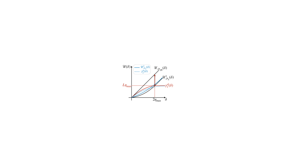
(a) Median	(b) Mean	(c) Distributional

Figure 3: Extrapolation uncertainty and extrapability gains. The gains for the mean and the distribution depend on the specific noise distribution and here we take $\eta\sim\mathrm{Unif}[-\eta_{\max},\eta_{\max}]$ as an example. Black lines represent extrapolation uncertainty; red lines are extrapability gains; red arrows represent the maximum extrapability gains.

We illustrate the theoretical formulas of extrapability gains in Figure 3. In summary, all the extrapability gains for the median, the mean, and the distribution are positive for all $\delta>0$ (except for one case of the distributional extrapability gain with the Wasserstein-$\infty$ distance). This indicates that engression has strictly lower extrapolation uncertainty across the entire real line. Notably, the maximum extrapability gains for the median, mean, and the distribution (with $\ell=1$) are the same. However, the maximum extrapability gain is achieved later for the mean and distribution than for the median. The reason is because the mean and distribution also rely on the higher (or even extreme) quantiles, for which engression has larger extrapolation uncertainty than that for the median. For distributional extrapability, when $1<\ell<\infty$, the gain becomes smaller than the one measured with $\ell=1$, but it still remains positive and achieves the same maximum gain at infinity. The extreme case of $\ell=\infty$, however, corresponds to the only measure under which engression does not show an advantage over baseline methods but performs identically.

4 Finite-sample analysis

We study the finite-sample behaviour of the engression estimator. We first derive finite-sample bounds for parameter estimation and out-of-support prediction under a special case of quadratic models when the pre-ANM is either well- or misspecified. Then we present the consistency results for general monotone and Lipschitz models.

4.1 Quadratic models

Consider the following quadratic pre-ANM class

$$\{\beta_{0}+\beta_{1}(x+\eta)+\beta_{2}(x+\eta)^{2}:\beta=(\beta_{0},\beta_{1},\beta_{2})\in\mathcal{B},\eta\sim P_{\eta}\in\mathcal{P}_{\eta}\},$$ (13)

where the covariate $x$ and noise variable $\eta$ are univariate, $\mathcal{B}\subseteq\mathbb{R}^{3}$ is a bounded parameter space such that $\beta_{1}\beta_{2}>0$, and $\mathcal{P}_{\eta}$ is a class of noise distributions. As such, this is a semiparametric model with a finite-dimensional parameter $\beta$ and infinite-dimensional component $\eta$. Assume all distributions in $\mathcal{P}_{\eta}$ are symmetric with a bounded support $[-\eta_{\max},\eta_{\max}]$. Assume the density of $Y=\beta_{0}+\beta_{1}(x+\eta)+\beta_{2}(x+\eta)^{2}$, denoted by $p_{\beta,\eta}(y|x)$, is uniformly bounded away from 0, i.e.

$$b:=\inf_{\begin{subarray}{c}x\in\mathcal{X},\beta\in\mathcal{B},\\ \eta\sim P_{\eta}\in\mathcal{P}_{\eta}\end{subarray}}p_{\beta,\eta}(y|x)>0.$$ (14)

Consider the extreme case where the covariate $X$ takes only two values during training, i.e. with the training support $\mathcal{X}=\{x_{1},x_{2}\}$, where $0<x_{1}<x_{2}$; assume $x_{1}>\eta_{\max}$ and that $X$ takes each value with probability $0.5$. The training data consists of $(x_{1},Y_{1,i}),i=1,\dots,n$ and $(x_{2},Y_{2,i}),i=1,\dots,n$. As we focus on the statistical behaviour concerning the sample size $n$ and one can in principle generate as many samples of the noise variable as possible without the worry of computational complexity, we assume the noise sample size $m$ in (10) tends to infinity. Denote the engression estimator in (10) based on the above sample by $\hat{\beta}=(\hat{\beta}_{0},\hat{\beta}_{1},\hat{\beta}_{2})$ and $\hat{\eta}$.

We are interested in predicting the conditional mean or quantile of $Y$ given $X=x$ for any point $x\in\mathbb{R}$, particularly those lying outside the support $\mathcal{X}$.

4.1.1 Well-specified pre-ANM

We first consider the case where the true data generating model is a pre-ANM, so that the pre-ANM class (13) is well specified. Specifically, let $\beta^{\star}=(\beta^{\star}_{0},\beta^{\star}_{1},\beta^{\star}_{2})\in\mathcal{B}$ be the true parameter and $\eta^{\star}\sim P^{\star}_{\eta}\in\mathcal{P}_{\eta}$ be the true noise variable.

We first show the failure in extrapolation of $L_{2}$ regression (3) and quantile regression (4) among the model class $\{\beta_{0}+\beta_{1}x+\beta_{2}x^{2}:\beta\in\mathcal{B}\}$. Define the set of $L_{2}$ regression estimators by

$$\mathcal{B}^{\mu}=\operatorname*{argmin}_{\beta}\frac{1}{2n}\sum_{j=1}^{2}\sum_{i=1}^{n}[Y_{j,i}-(\beta_{0}+\beta_{1}x_{j}+\beta_{2}x_{j}^{2})]^{2}$$

and the set of quantile regression estimators given a level $\alpha$ by

$$\mathcal{B}^{\textsl{q}}_{\alpha}=\operatorname*{argmin}_{\beta}\frac{1}{2n}\sum_{j=1}^{2}\sum_{i=1}^{n}\rho_{\alpha}(Y_{j,i}-(\beta_{0}+\beta_{1}x_{j}+\beta_{2}x_{j}^{2})).$$

Note that given two values $x_{1},x_{2}$ of the covariate, both $L_{2}$ regression and quantile regression do not have a unique solution, i.e. sets $\mathcal{B}^{\dagger}$ and $\mathcal{B}^{\ddagger}$ are not singleton. Let $\mu^{\star}(x)$ be the true conditional mean of $Y$ given $X=x$ and $q^{\star}_{\alpha}(x)$ be the true conditional $\alpha$-quantile.

The following proposition suggests that $L_{2}$ regression and quantile regression yield arbitrarily large errors for conditional mean and quantile prediction for out-of-support data. The proof is given in Appendix B.2.

Proposition 2.

For all $x\notin\mathcal{X}$, we have

$$\sup_{\beta\in\mathcal{B}^{\mu}}\mathbb{E}[(Y-(\beta_{0}+\beta_{1}x+\beta_{2}x^{2}))^{2}]=\infty,$$

and for all $\alpha\in[0,1]$

$$\sup_{\beta\in\mathcal{B}^{\textsl{q}}_{\alpha}}|(q^{\star}_{\alpha}(x)-(\beta_{0}+\beta_{1}x+\beta_{2}x^{2})|=\infty.$$

Now we turn to engression. Let $\hat{q}_{\alpha}(x)$ be the engression estimator for the conditional $\alpha$-quantile of $Y$ given $X=x$, which is defined as the $\alpha$-quantile of $\hat{\beta}_{0}+\hat{\beta}_{1}(x+\hat{\eta})+\hat{\beta}_{2}(x+\hat{\eta})^{2}$ in terms of $\hat{\eta}$. Let $\hat{\mu}(x)$ be the engression estimator for the conditional mean, defined as $\mathbb{E}_{\hat{\eta}}\big{[}\hat{\beta}_{0}+\hat{\beta}_{1}(x+\hat{\eta})+\hat{\beta}_{2}(x+\hat{\eta})^{2}\big{]}$. Theorem 5 presents the finite-sample bounds for estimation errors of the parameter as well as the conditional mean and quantiles. Notably, in contrast to the failure of $L_{2}$ regression and quantile regression, our engression yields consistent estimators for the conditional mean and quantiles for data points both within or outside the support, as shown in (16) and (17). The proof is given in Appendix B.3.

Theorem 5.

Let $\delta>0$. Under the setting posited above, with probability exceeding $1-\delta$, we have

$$\|\hat{\beta}-\beta^{\star}\|\leq\frac{C_{1}}{(x_{2}-x_{1})b^{\frac{2}{3}}}\left(\frac{\log(2/\delta)}{n}\right)^{\frac{1}{3}},$$ (15)

where $b$ is defined in (14), and $C_{1}$ is a constant depending on the parameter space $\mathcal{B}$ and the noise level $\eta_{\max}$. In addition, for any $x\in\mathbb{R}$, it holds with probability exceeding $1-\delta$ that

$$(\hat{\mu}(x)-\mu^{\star}(x))^{2}\leq C_{2}\max\{1,|x|,x^{2}\}\left(\frac{\log(2/\delta)}{n}\right)^{\frac{2}{3}},$$ (16)

where $C_{2}<\infty$ is a constant independent of $x$. For any $x\in\mathbb{R}$ and $\alpha\in[0,1]$, it holds with probability exceeding $1-\delta$ that

$$|\hat{q}_{\alpha}(x)-q^{\star}_{\alpha}(x)|\leq C_{3}\max\{1,|x|,x^{2}\}|Q^{\eta^{\star}}_{\alpha}|\left(\frac{\log(2/\delta)}{n}\right)^{\frac{1}{3}}.$$ (17)

where $C_{3}<\infty$ is a constant independent of $\alpha$ and $x$.

Taking a closer look at the error rate for parameter estimation in (15), the constant is monotonically decreasing with respect to $x_{2}-x_{1}$, indicating that the engression estimator would yield faster convergence as the training support of the covariate becomes more diverse. Also the constant $C_{1}$ is in fact monotonically decreasing with respect to the noise level $\eta_{\max}$. In addition, the dependence of the rates for the conditional mean and quantile estimation suggest that it tends to be more challenging to extrapolate on a point farther away from training data or for extreme quantiles. These findings align with our previous theoretical results at the population level as well as the empirical observations presented below.

Furthermore, due to the nonparametric component $\eta$, engression yields a nonparametric rate of the order $\mathcal{O}(n^{-\frac{1}{3}})$. However, in this case, a simple modification of engression that enforces the conditional median to take the parametric form $\beta_{0}+\beta_{1}x+\beta_{2}x^{2}$ (e.g. by adding a regularisation term or imposing parametric assumptions on $\eta$) can lead to the parametric rate for $\beta$ and conditional median estimation. It remains an open problem whether engression can achieve a parametric rate more generally.

4.1.2 Misspecified pre-ANM

We further investigate the case with model misspecification, in particular, when the pre-ANM assumption, which plays a key role in engression, is violated. Consider the same setting as above with the only difference being that the training data is now assumed to be generated according to $Y=\beta^{\star}_{0}+\beta^{\star}_{1}x+\beta^{\star}_{2}x^{2}+\eta^{\star}$ which is in fact a post-ANM. However, we continue to adopt engression with the pre-ANM class defined in (13) which does not contain the true model.

The following theorem presents the bounds for the parametric component $\hat{\beta}$ of the engression estimator, which is proved in Appendix B.4.

Proposition 3.

Under the setting posited above, with probability exceeding $1-\delta$, we have

$$\max\big{\{}|\hat{\beta}_{0}-(\beta^{\star}_{0}-\beta^{\star}_{2}x_{1}x_{2})|,\ |\hat{\beta}_{1}-(\beta^{\star}_{1}+\beta^{\star}_{2}(x_{1}+x_{2}))|,\ |\hat{\beta}_{2}|\big{\}}\lesssim\left(\frac{\log(2/\delta)}{n}\right)^{\frac{1}{3}}.$$

We note that the engression estimator is generally inconsistent unless the true model is linear (i.e. $\beta^{\star}_{2}=0$), which is reasonable since the model is misspecified. More interestingly, engression still yields a unique solution, in contrast to the non-uniqueness of regression. Furthermore, engression leads approximately to a linear model with $\hat{\beta}_{2}\overset{p}{\to}0$ as $n\to\infty$. As we have only observations at two distinct values of the predictor variable, a linear fit seems to be a useful fallback option in case of model misspecification. In comparison, traditional regression methods again exhibit arbitrarily large errors outside the training support, as shown in Proposition 2.

4.2 General pre-ANMs

We extend the previous setting and focus on a general pre-ANM class $\{g(x+h(\varepsilon)):g\in\mathcal{G},h\in\mathcal{H}\}$ defined in Section 3 without the additional linear term. We consider a continuous support $\mathcal{X}=[x_{\min},x_{\max}]$ which is a bounded interval on $\mathbb{R}$. Without loss of generality, we assume that $\varepsilon\sim\mathrm{Unif}[0,1]$ and $\mathcal{H}$ is the same as posited in Section 3.2. Let $g^{\star}(x+h^{\star}(\varepsilon))$ be the true model. Let $n$ be the training sample size.

The following theorem states the consistency of the engression estimator $(\hat{g},\hat{h})$. Notably, the set of covariate values for which the consistency of $\hat{g}$ is achieved, i.e. $\tilde{\mathcal{X}}$, extends beyond the support up to a range depending on the noise level. In addition, the consistency of $\hat{h}$ implies that engression can consistently estimate the cdf of the noise distribution. The proof is given in Appendix B.5.

Theorem 6.

Assume the following conditions hold:

1. $x_{\max}-x_{\min}\geq\max\{|h^{\star}(1)|,|h^{\star}(0)|\}$.

2. $\mathcal{G}$ is uniformly Lipschitz and strictly monotone.

3. $X$ lies on grid points $x_{\min}=x_{0}<x_{1}<\dots<x_{m}=x_{\max}$, where $m=m(n)$ such that $m(n)\to\infty$, $m(n)/n\to 0$, and $\max_{i=1,\dots,m}|x_{i}-x_{i-1}|=o(m)$ as $n\to\infty$, and $\mathbb{P}(X=x_{i})\geq c/m$ for some $c>0$.

Then it holds for all $\tilde{x}\in\tilde{\mathcal{X}}:=\{x+h^{\star}(\varepsilon):x\in\mathcal{X},\varepsilon\in[0,1]\}$ and $\varepsilon\in[0,1]$ that

$$\hat{g}(\tilde{x})\overset{p}{\to}g^{\star}(\tilde{x})\quad\text{and}\quad\hat{h}(\varepsilon)\overset{p}{\to}h^{\star}(\varepsilon)\quad\text{as $n\to\infty$.}$$

Condition (B1) requires the training support of the covariate exceed the noise level. Condition (B2) imposes assumptions on the function class. It is worth noting that with the Lipschitz condition, we establish the consistency for covariate values outside the support, which traditional regression approaches, however, do not attain. For example, under the same assumptions, $L_{1}$ regression consistently exhibits an error for conditional median estimation on out-of-support data that scales linearly with respect to the distance away from the support boundary, as indicated in Theorem 2. Condition (B3) is a technical assumption for simplifying the analysis and we think the same results could be shown for $X$ with a general continuous density that is bounded away from 0.

5 Empirical results

We start with simulated scenarios without model misspecification in Section 5.1 and then extend to the real-world scenarios without guarantees for the fulfillment of the model assumptions in Section 5.2.

5.1 Simulations

We simulate data from a heteroscedastic noise model that falls into the pre-ANM class in (11), with details given in Table 1. In all settings, the training data are supported on a bounded set and the true functions are nonlinear outside the support. We compare engression to the traditional $L_{1}$ and $L_{2}$ regression; for all methods, we use the identical implementation setups including architectures of neural networks and all hyperparameters of the optimisation algorithm. For each setting, we randomly simulate data and apply the methods with random initialisation, which is repeated for 20 times. All the experimental details are described in Appendix E.

Table 1: Simulation settings. In all settings, the training data are supported on a bounded set within the boundary value $x_{\max}=2$. With a finite sample, the noise also has a bounded support with roughly $\eta_{\max}\approx 2$ (approximately 97.5% quantile of a standard Gaussian). All functions $g^{\star}$ are nonlinear outside the support except that the softplus function is approximately linear as $x$ grows large.

Name	$g^{\star}(\cdot)$	$X$	$\eta$
softplus	$g^{\star}(x)=\log(1+e^{x})$	Unif$[-2,2]$	$\mathcal{N}(0,1)$
square	$g^{\star}(x)=(x_{+})^{2}/2$	Unif$[0,2]$	$\mathcal{N}(0,1)$
cubic	$g^{\star}(x)=x^{3}/3$	Unif$[-2,2]$	$\mathcal{N}(0,1.1^{2})$
log	$g^{\star}(x)=\begin{cases}\frac{x-2}{3}+\log(3)&x\leq 2\\ \log(x)&x>2\end{cases}$	Unif$[0,2]$	$\mathcal{N}(0,1)$

We are interested in the performance of the estimated models outside the training support. To evaluate this, we use both qualitative visualisations and quantitative metrics. While we focus here on extrapolation beyond the larger end of the support for convenience, we expect similar phenomena to happen for the smaller side as well; we investigate extrapolation on both ends of the training support in real-data experiments.

Figure 4 visualises the overall performance of different methods, where we plot the fitted curves as well as the true function. Here we are concerned with the estimation of the conditional median and mean functions of $Y$ given $X=x$. The true median function is given by $g^{\star}(x)$, while the true mean function is given by $\mathbb{E}_{\eta}[g^{\star}(x+\eta)]$, which is estimated based on the sampling $10^{5}$ i.i.d. draws of $\eta$. The engression estimators for the median and mean are estimated from 512 samples from the engression model for each $x$. We observe that within the training support, all methods perform almost perfectly. However, once going beyond the support, $L_{1}$ and $L_{2}$ regression fail drastically and tend to produce uncontrollable predictions, resulting in a huge spread that represents roughly the extrapolation uncertainty. In contrast, the extrapolation uncertainty, as shown by the shaded area, of engression is significantly smaller. Particularly when $x\leq 4$, which roughly corresponds to $x\leq x_{\max}+\eta_{\max}$, engression leads to nearly 0 extrapolation uncertainty for the conditional median, which supports our local extrapability results in Section 3.3. The extrapolation uncertainty of engression for the conditional mean tends to be slightly higher than that for the conditional median, which coincides with the results in Theorems 2 and 3.

	Conditional median		Conditional mean
	Engression	$L_{1}$ regression	Engression	$L_{2}$ regression
softplus
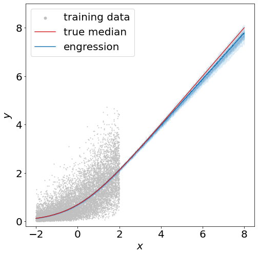
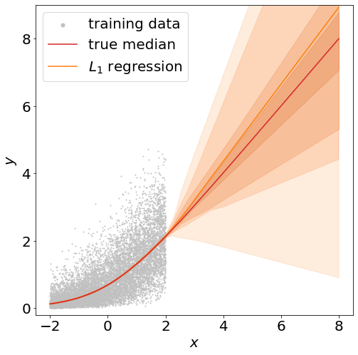
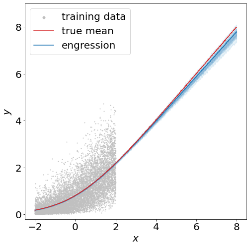
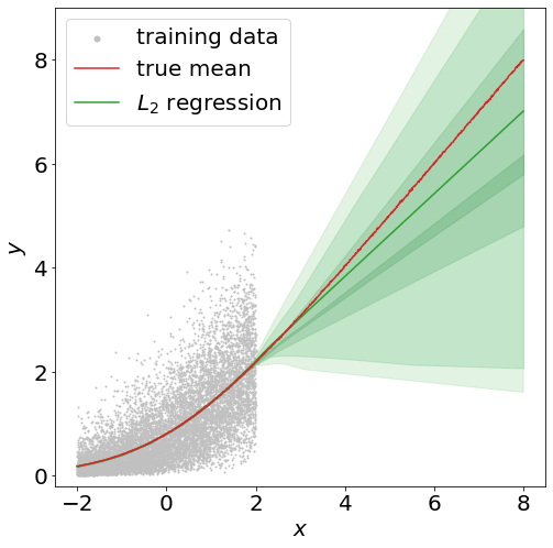
square
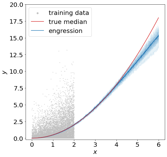
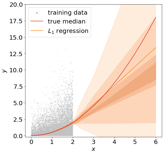
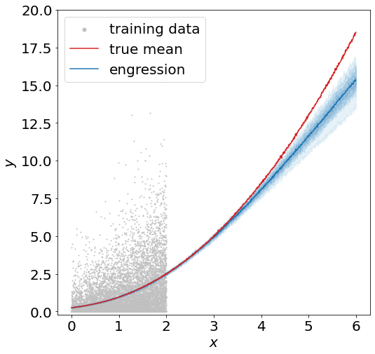
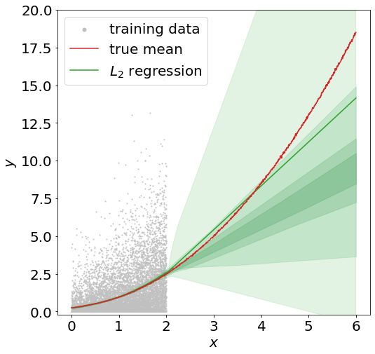
cubic
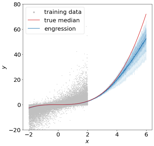
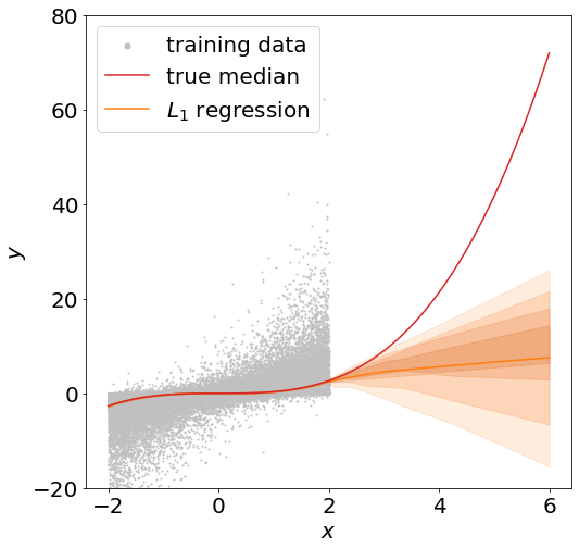
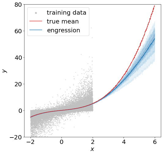
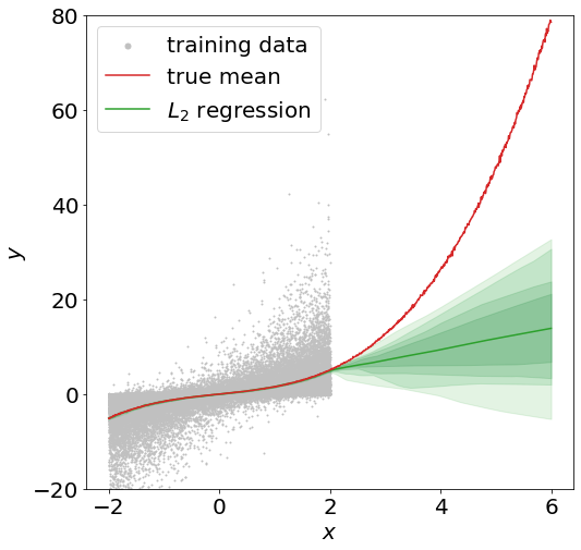
log

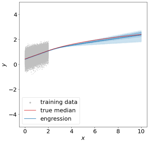
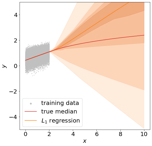
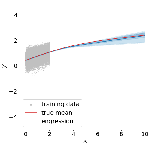
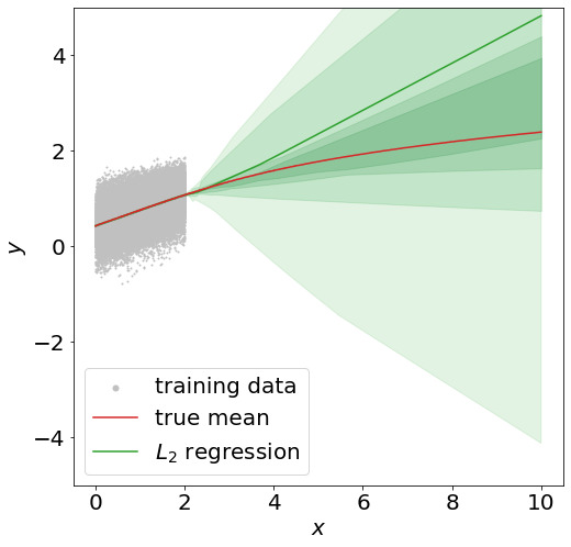
Figure 4: The estimated conditional medians and means of different methods in all simulation settings. Each figure consists of the estimated functions for 20 random repetitions (whose 10% to 90% quantiles are plotted in graduated colors with the darkest curve in the middle representing the mean of the 20 estimated mean functions), the true function, and training data.

softplus	square	cubic	log

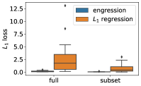
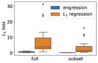
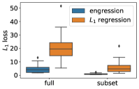
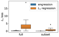
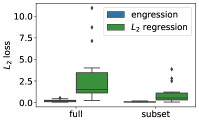
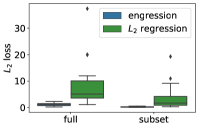
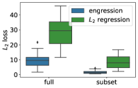
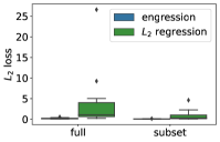
Figure 5: Average performance on out-of-support data. The top row shows the $L_{1}$ loss for conditional median estimation; the bottom row shows the $L_{2}$ loss for conditional mean estimation.

square	log

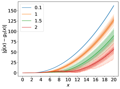
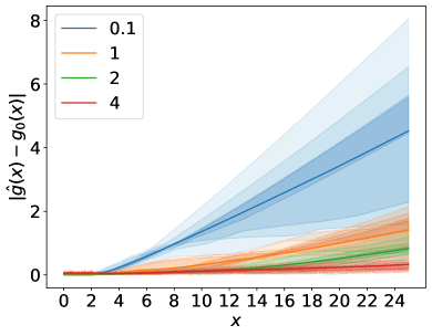
Figure 6: Extrapolation performance for varying noise levels. The training support is $[0,2]$. On the $y$-axis we compute the pointwise absolute error between the estimated and true conditional medians for each $x$ inside or outside the support. Each colour stands for a particular standard deviation of the noise $\eta$.

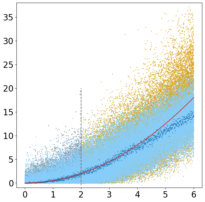
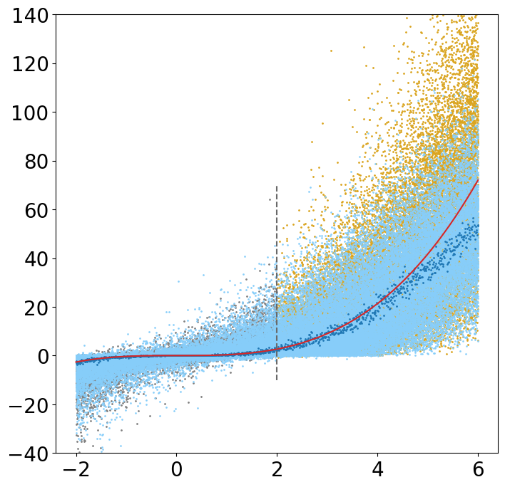
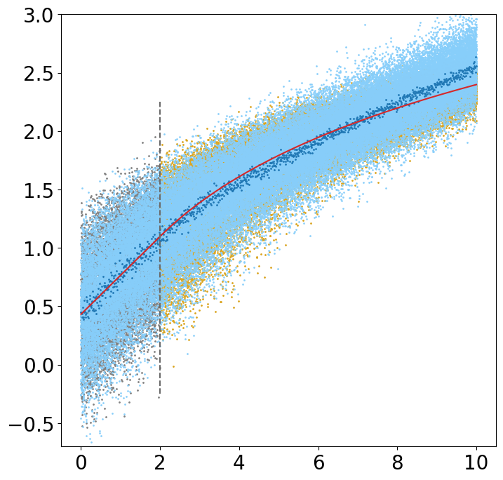
softplus	square	cubic	log

Figure 7: Data generated from the true model and engression model within and outside the training support. The dashed vertical lines are the boundaries of training and test data. For each $x$, $\hat{g}(x)$ is obtained by the empirical median of 64 samples from the engression model.

In addition to the visual illustrations, we quantitatively evaluate the conditional median estimation using the $L_{1}$ loss and the conditional mean estimation using the $L_{2}$ loss. Both metrics are computed according to $X$ following a uniform distribution on two (sub)sets outside the training support: a subset $[x_{\max},x_{\max}+\eta_{\max}]$ on which engression consistently recover the true (median) function by Proposition 1, and the ‘full’ test set which goes further beyond the local extrapable boundary $x_{\max}+\eta_{\max}$. The metrics for the 20 repetitions are reported via boxplots in Figure 5. These numerical results further demonstrate the substantial advantages of engression in extrapolation outside the training support for the conditional mean or median function.

Additionally, we illustrate how engression can take advantage of higher noise levels. In the simulation settings for square and log, we experiment with various variance levels for the noise $\eta$. As depicted in Figure 6, with an increase in the noise level, engression tends to extrapolate over a broader range until the prediction curve begins to diverge from the true function. This observation supports Proposition 1, which asserts that engression can consistently recover the true function up to a boundary that becomes less restrictive with an increasing noise level.

Finally, we investigate how well engression fits the entire conditional distribution of $Y|X$ via sampling. Figure 7 presents the scatterplots of the true data and data generated from the engression model. Inside the training support, engression captures exactly the true conditional distribution, generating data identically distributed as the true data. Outside the support, the estimated distribution still exhibits a large overlap with the true distribution at the beginning while eventually starts to deviate from the truth, except the softplus case where engression appears to produce linear extrapolation that matches the true one.

5.2 Real data experiments

We apply engression to an extensive range of real data sets spanning various domains such as climate science, biology, ecology, public health, and more. We compare engression with traditional prediction methods, including $L_{1}$ regression and $L_{2}$ regression with neural networks, linear quantile regression (LQR) (Koenker and Bassett,, 1978; Koenker,, 2005), linear $L_{2}$ regression (LR), and quantile regression forest (QRF) (Meinshausen,, 2006). Our investigation begins with large-scale experiments on univariate prediction, where the primary goal is to assess the wide applicability and validity of engression across different domains. Furthermore, we extend our evaluation to multivariate prediction and prediction intervals, showcasing the versatility of engression in various prediction tasks. We provide descriptions of the data sets and all details about hyperparameter and experimental settings in Appendix E.

5.2.1 Univariate prediction

We conduct pairwise predictions on data sets from a variety of fields, which results in 30 pairs of variables and 59 univariate prediction tasks, accomplished by switching the roles of the predictor and response variables (with one discrete variable being exclusively considered as the response). For each prediction task, we partition the training and test data based on the quantiles of the predictor, specifically at the 0.3, 0.4, 0.5, 0.6, 0.7 quantiles, and designate the smaller or larger portion as the training sample. This way, all the test data lie outside the training support and we encounter diverse patterns of training and test data. Hence, we have a total of 590 unique data configurations, each representing a specific combination of the data set, predictor/response variables, and data partitioning.

Additionally, we utilise the same range of hyperparameter settings for NN-based methods, including engression and $L_{1}$ or $L_{2}$ regression. This range includes various combinations of learning rates, numbers of training iterations, layers, and neurons per layer. In each data configuration, we experiment with 18 unique hyperparameter settings, resulting in a total of 31,860 models generated by the three NN-based methods. Each model represents an aggregate of 10 models acquired through 10-fold cross-validation (CV). Regarding evaluation, we report both the average performance across all hyperparameter settings and the performance for the hyperparameter setting that yields the best CV metric. Specifically, for engression, $L_{1}$ regression, and $L_{2}$ regression, we employ the energy loss, $L_{1}$ loss, and $L_{2}$ loss as the validation metrics, respectively. This strategy ensures a fair and consistent foundation for comparison and mitigates potential bias originating from hyperparameter tuning.

Our main evaluation metric is the $L_{2}$ loss on the out-of-support test data which reflects the extrapolation performance in such practical scenarios. Table 2 demonstrates the comparative performance of each method across various data configurations. Engression consistently stands out as one of the top methods for the most of the data settings. In contrast, other nonlinear approaches, including $L_{1}$ and $L_{2}$ NN regression and quantile regression forests, significantly underperform compared to engression, which aligns with our theoretical and simulation findings presented earlier. Linear models, while inferior to engression, often rank second, possibly because the out-of-support patterns on real-world data are relatively close to linearity. In addition, it is worth noting that the average performance of engression across all hyperparameter settings is already superior compared to other methods, although model selection via cross validation can further magnify the advantage.

Table 2: Proportion (in percentage) of the data configurations for each method with the out-of-support $L_{2}$ loss exceeding the best loss by a certain percentage given in the first column. For example, the first number in the table, 79, means that on 79% of all data configurations, the test $L_{2}$ loss of engression (averaging across all hyperparameter settings) exceeds the minimum test $L_{2}$ loss among all approaches for the same data configuration by 1%. The smaller the numbers, the better the method is. For NN-based methods, including engression and $L_{1}$ and $L_{2}$ regression, we report both the average performance across all hyperparameter settings or the best performance according to the CV metric.

exceeding	engression		$L_{1}$ regression		$L_{2}$ regression		LQR	LR	QRF
percentage	average	CV	average	CV	average	CV
1%	79	55	98	72	97	82	85	81	93
3%	65	44	95	63	93	72	78	71	91
10%	35	28	86	44	83	56	61	54	83
30%	14	12	64	22	60	41	38	34	62
100%	2	3	26	9	21	25	13	11	28

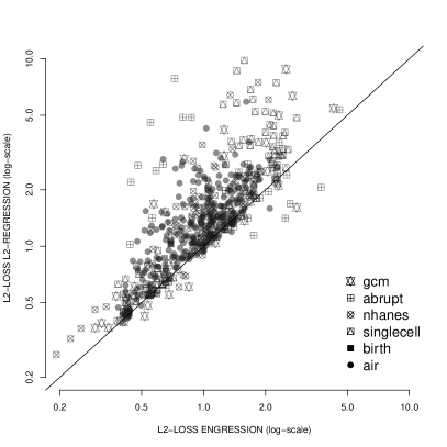
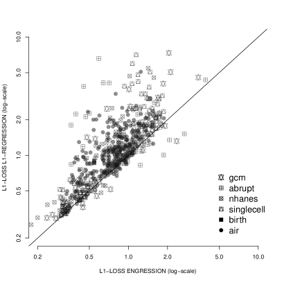
(a) $L_{2}$ loss	(b) $L_{1}$ loss

Figure 8: Out-of-support losses (in log-scale) of engression and regression for various data configurations, averaging over all hyperparameter settings.

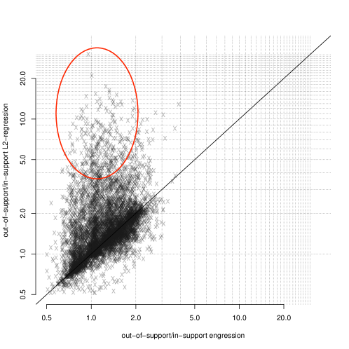
Figure 9: The ratio (in log-scale) between out-of-support and in-support $L_{2}$ losses of engression and regression for all hyperparameter settings on the air pollution data.

Moreover, we show a more detailed comparison between engression and regression, both always using the same architecture of the neural networks. As demonstrated in Figure 8, engression consistently surpasses $L_{1}$ and $L_{2}$ regression in terms of the $L_{1}$ and $L_{2}$ loss on test data that fall outside the support, respectively. This is true even though these losses are specifically optimised by the regression methods on the training data.

Beyond the absolute evaluation of performance on data outside the support, we also scrutinise the relative performance between predictions made within and beyond the support. We utilise the $L_{2}$ loss on the omitted folds in cross-validation to gauge the performance within the support, which aids in sidestepping potential overfitting effects. Figure 9 shows the ratio between the $L_{2}$ losses for predictions made outside the support versus those made within it for both methods. We arrive at two key observations. Firstly, the ratios of engression are typically around 1, suggesting negligible performance degradation when transitioning from within-support to outside-support prediction. In contrast, regression tends to encounter more pronounced difficulties when extending beyond the training support, as illustrated by the generally larger ratios (note the log-scaling on the plot). In particular, there exist several instances where engression maintains comparable performance levels both within and outside the support, whereas regression exhibits a substantial increase in loss for predictions outside the support compared to those within it, as shown in the red circle. This further highlights the superior extrapolation performance of engression. Additionally, it should be noted that we plot the performance for all hyperparameter settings, and engression demonstrates less variance in performance compared to regression. This implies that engression displays greater robustness across a range of hyperparameter configurations.

The large-scale experimental study comprehensively demonstrates the remarkable performance of engression in out-of-support prediction. The empirical results suggest that engression is suitable for a wide range of real data and offers practitioners an alternative modelling choice for practical data analysis. Furthermore, it is worth noting that for each pair of variables across all data sets, we include the prediction tasks in both directions, taking either of them as the response and the other one as the predictor and the other way round. This ensures that at least in one of these two directions, the assumption on the pre-ANM is not fully fulfilled, unless the relationship is linear. Considering this, the observation that engression works well across all these data set configurations indicates the satisfying robustness of engression under model misspecification, which makes it even more widely applicable in real scenarios.

5.2.2 Multivariate prediction

Next, we demonstrate the performance of engression in multivariate prediction through two data sets. (While we focus here on the setting of multivariate predictors and univariate outcome, the method is also directly applicable to multivariate outcomes, which is implemented in our software.) The air quality data comprises measurements of five pollutants and three meteorological covariates. For the prediction task, we select one pollutant as the response variable and utilise the remaining variables as predictors. The NHANES data set includes the total activity count (TAC), sedentary time (ST), body mass index (BMI), and age, where we consider predicting the TAC from the remaining three variables. The data is split into training and test sets based on the median of one of the predictors. We evaluate the performance by the $L_{2}$ losses on both training and test data.

Engression	NN regression	Linear regression
(0.0798, 0.1662)	(0.0099, 0.7670)	(0.1639, 0.5022)
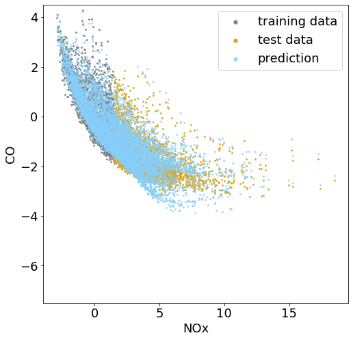
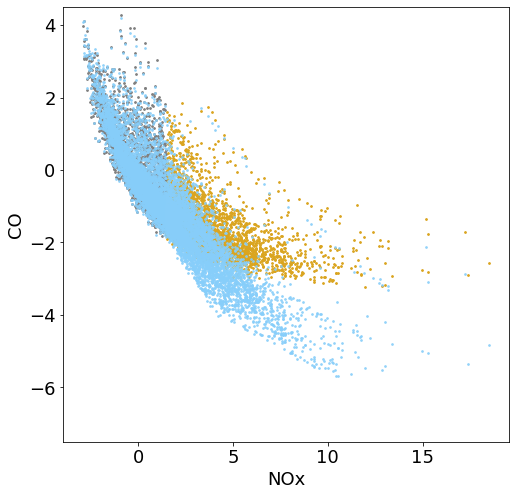
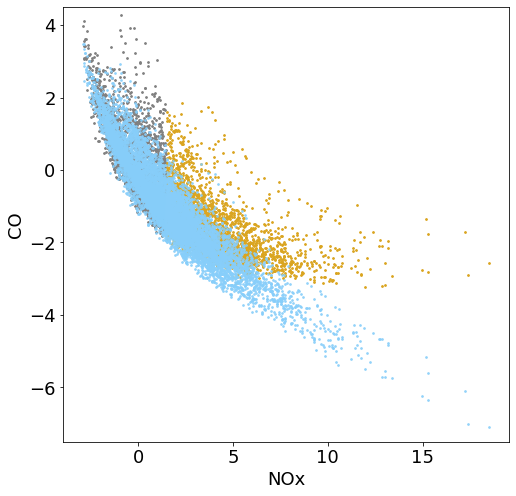
(0.1687, 0.2096)	(0.0017, 2.9041)	(0.3041, 1.4730)
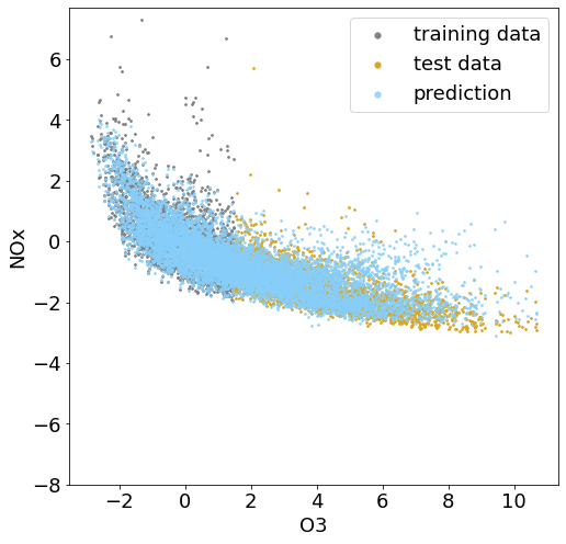
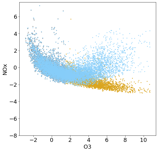
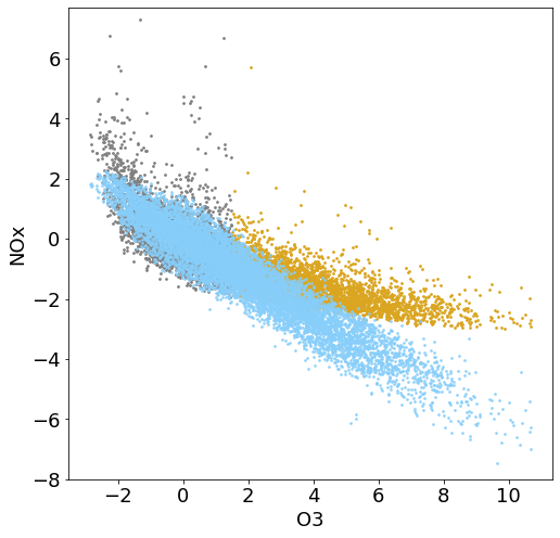
(0.1267, 0.6392)	(0.0021, 1.8257)	(0.3462, 0.9700)

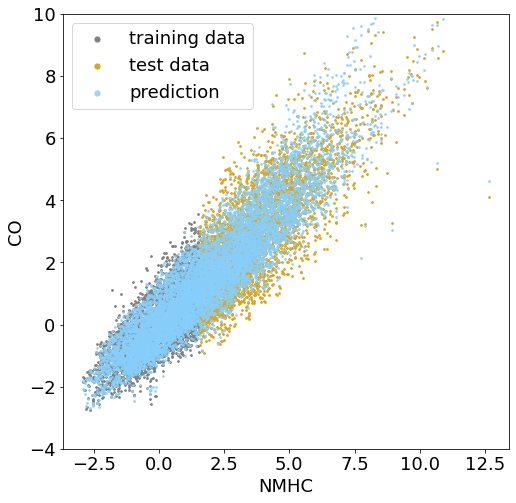
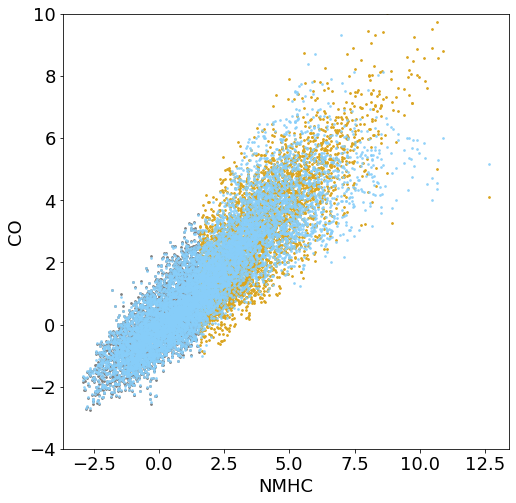
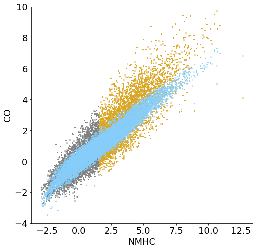
Figure 10: Results for multivariate prediction on the air quality data. Each row shows a predictor-response pair; each column is for a method. In each plot, the variable on the x-axis is used to split the training and test data at its median. The numbers in the parenthesis above each plot are the training and test $L_{2}$ losses, respectively. The spread in the predictions arises due to the presence of other predictor variables in this multivariate prediction.

Engression	NN regression	Linear regression
(0.3632, 0.1735)	(0.2087, 3.8117)	(0.3741, 0.8245)
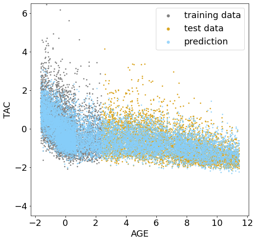
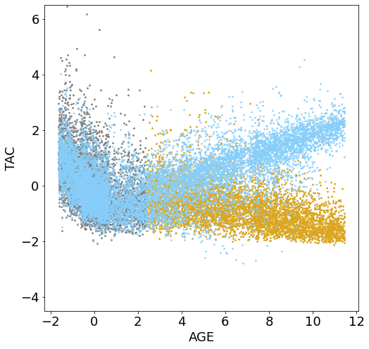
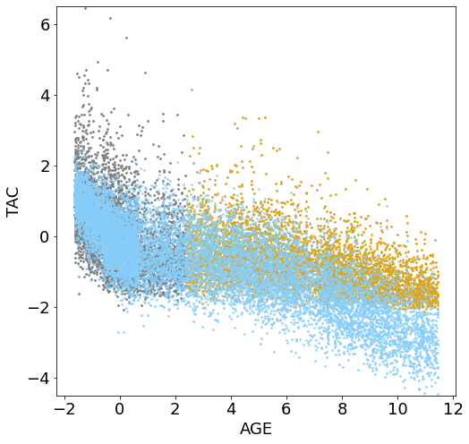
(0.4500, 0.1838)	(0.3393, 0.6753)	(0.4646, 0.4223)
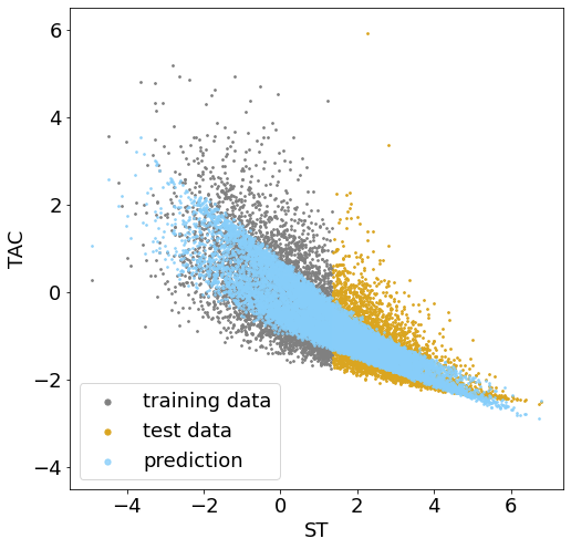
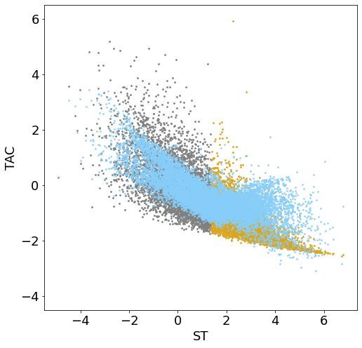
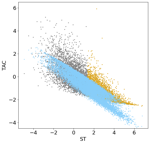
(0.3156, 0.1743)	(0.2095, 1.0541)	(0.3375, 0.2532)

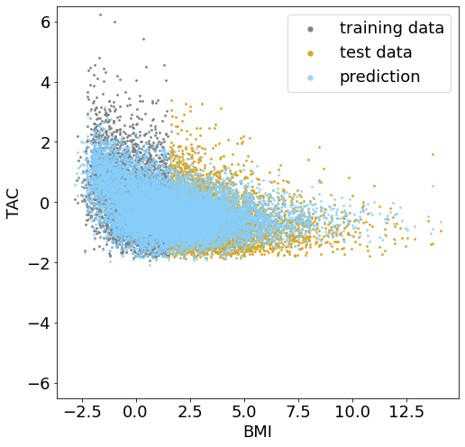
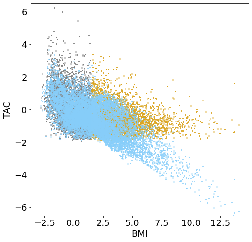
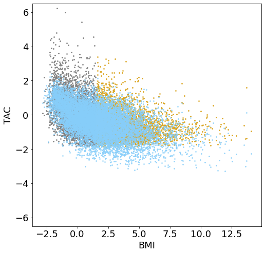
Figure 11: Same plot for the NHANES data.

In Figures 10-11, we visualise the results by plotting the response variable against the predictor $i$ that is used for splitting training and test data. We include both the true data points and the prediction of $\mathbb{E}[Y|X_{i}=x_{i},X_{-i}]$, where $X_{-i}$ denotes the set of remaining predictors excluding $X_{i}$. In most scenarios, the marginal relations between the response and the predictor are nonlinear. We observe that linear regression tends to show predominantly linear extrapolations when visualised univariately. However, nonlinear effects can surface in the results, originating from nonlinear dependencies between the depicted predictor variables and the other variables present in the data set. On the other hand, NN $L_{2}$ regression, while consistently having the smallest training loss, fails to extrapolate reliably, resulting in a significantly larger test loss. In comparison, engression outperforms both linear regression and NN regression. It achieves a lower training loss than linear regression, owing to the expressiveness of the NN class. More importantly, engression often maintains a strong performance on out-of-support test data, significantly surpassing the other two approaches.

In the bottom row of Figure 10, the marginal relationship appears to be almost linear, with a slight presence of heteroscedasticity. In this case, all methods appear to provide reasonable predictions visually. However, when evaluated quantitatively, engression exhibits a much lower test loss. In fact, although the marginal relationship between CO and NMHC is approximately linear, the relationships between CO and other predictors, like NOx (as shown in the top row) are nonlinear. Thus, predicting CO based on multiple predictors still requires nonlinear extrapolation in which engression excels, although the advantage lies in the other predictors and is not explicitly reflected in the marginal relationship between CO and NMHC as shown in the plots.

In summary, these empirical findings suggest the potential of engression in multivariate prediction. Thus, it is worthwhile to delve deeper into the theoretical underpinnings of engression in multivariate scenarios in future research.

5.2.3 Prediction intervals

Engression can also be applied to construct prediction intervals based on the conditional quantile estimations. Specifically, we compute the 2.5% and 97.5% quantiles of the estimated conditional distribution from engression and obtain the 95% prediction intervals based on them. Note that we do not account for the estimation uncertainty arising due to a finite sample size. We use linear quantile regression and quantile regression forests as baseline methods, where the intervals are derived based on the estimated quantiles. We also consider standard prediction intervals with linear $L_{2}$ regression for Gaussian errors as another baseline.

In Figure 12, we visualise the 95% prediction intervals on three data sets, along with the average coverage probabilities. We observe that for engression and most baseline methods, about 95% of all training data points fall within the 95% prediction intervals. However, when it comes to out-of-support test data, only the prediction intervals obtained through engression attain good coverage, while the other three methods exhibit significantly lower coverage rates. For instance, for the GCM data where we predict the global mean temperature from the radiation, their relationship is nonlinear during training while extrapolating linearly during test. Linear methods, though obtaining the best linear fits for the training distribution, provide misleading prediction intervals that cover the test data poorly. In comparison, engression successfully captures the pattern outside the support, leading to prediction intervals with decent coverage. These results align with the extrapability guarantee of engression for quantile estimation in Corollary 1, whereas the failure of other methods is mainly due to unreliable estimations of the quantiles (for QR and QRF) or the mean (for LR) outside the support.

It is notable that conformal prediction (Shafer and Vovk,, 2008; Lei et al.,, 2018) can also be used to construct prediction intervals. Nonetheless, when it comes to extrapolation, the residuals of a regression model at data points that fall outside the support would generally not fulfill the exchangeability assumption necessary for conformal prediction as we are operating outside the support of the training distribution. Consequently, adapting conformal prediction to ensure coverage guarantees for out-of-support predictions is not a straightforward task.

	Engression	Linear regression	Linear quantile regression	quantile regression forest
GCM
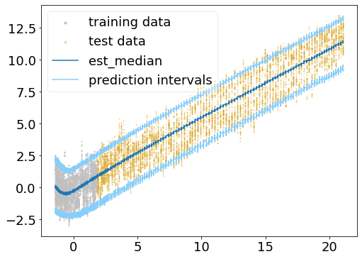
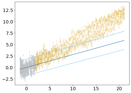
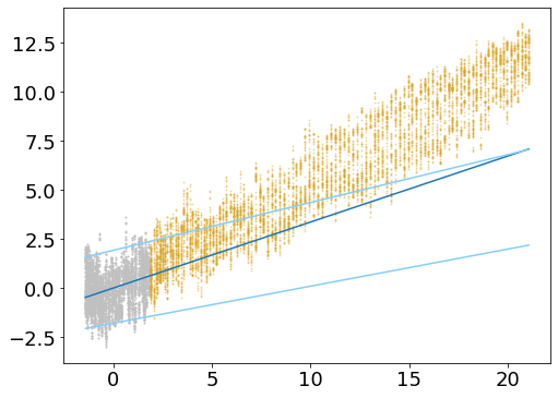
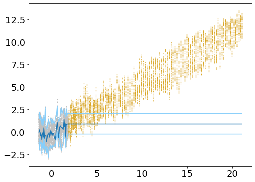
	(0.964, 0.917)	(0.937, 0.366)	(0.950, 0.333)	(0.938, 0.152)
Air
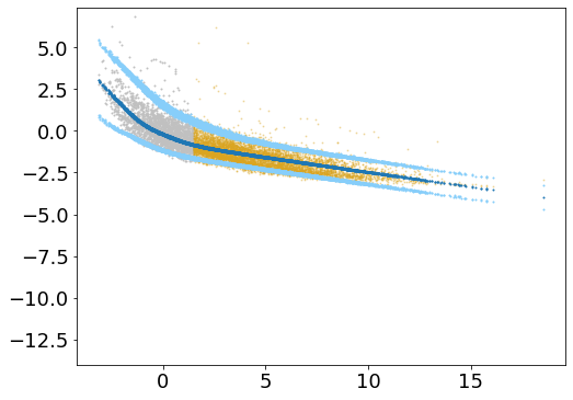
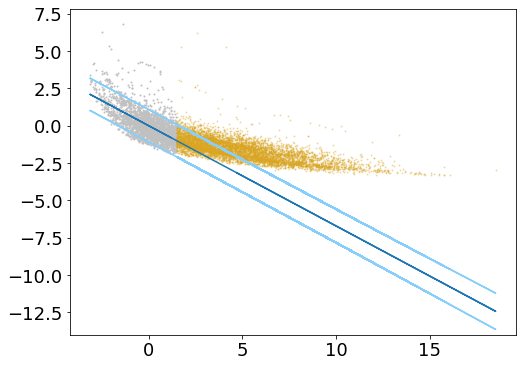
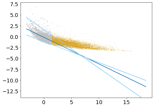
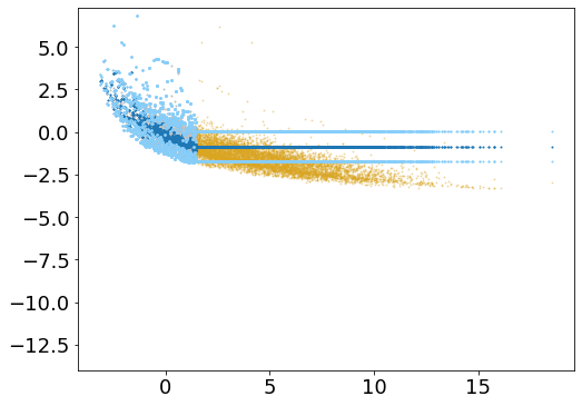
	(0.946, 0.916)	(0.900, 0.363)	(0.951, 0.313)	(0.995, 0.559)
NHANES
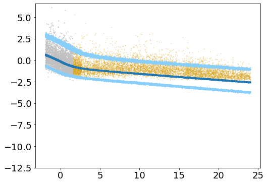
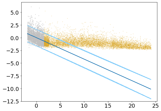
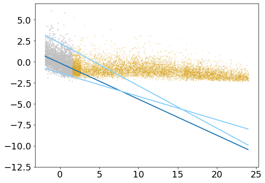
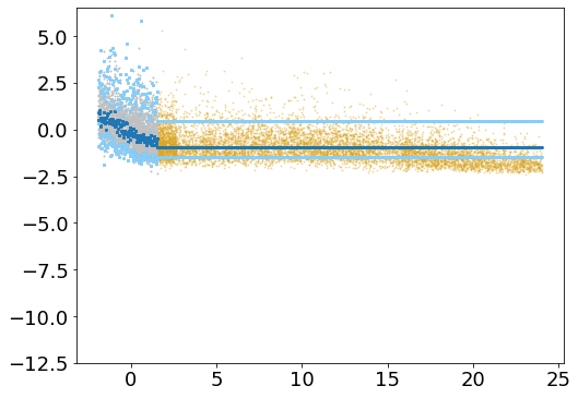
	(0.951, 0.885)	(0.939, 0.264)	(0.951, 0.272)	(0.962, 0.690)

Figure 12: Prediction intervals. Each row shows the results on a data set; each column is for a method. The numbers in the parenthesis under each plot are the average coverage probabilities of the prediction intervals on training and test data, respectively.

6 Discussion

Our paper introduces a novel framework for regression aimed at enhancing the ability of nonlinear regression models to extrapolate beyond the support of the training data. This need arises from the limitations of existing regression models: linear models, while capable of extrapolation, are a rather restrictive class, offering limited flexibility. In contrast, nonlinear regression models, such as tree ensembles and neural networks, suffer from their own deficiencies when it comes to extrapolation. Tree ensembles provide a constant prediction when extending beyond of the support, which may not be accurate in many contexts. Neural networks, on the other hand, tend to be uncontrollable when used for extrapolation.

To overcome these drawbacks, our approach incorporates two key components: a pre-additive noise model and a distributional fit. The advantage of a pre-ANM model class is, in simple terms, that it reveals the nonlinearities outside of the training support of the predictor variables. This benefit can only be captured, however, if we fit the full conditional distribution. Importantly, we have shown that both ingredients (i.e. pre-ANM models and distributional fitting) are necessary for extrapolation and that neither adopting a post-ANM nor fitting merely the mean or quantiles would attain the same merits.

The usefulness and robustness of our proposed engression methodology are demonstrated through theoretical proofs and empirical evidence. Our theoretical results show a significant improvement in extrapolation when using the population version of our approach. Interestingly, the range to which we can extrapolate benefits from a high noise level. In addition, we have studied finite-sample bounds for some specific settings, which shows the possibility to extrapolate beyond the support of the finite training data if the pre-additive noise model is correct. Even when the pre-additive noise assumption is incorrect and the true model proves to be a post-additive model with homoscedastic noise, the model yield by engression defaults to a linear extrapolation, thereby ensuring a useful baseline performance. On the other hand, our empirical results validate our theoretical findings and show the robustness and accuracy of engression in various regression tasks.

Appendix A Proofs of Section 3

A.1 Proof of examples in Section 3.1

Proof of Example 1.

Let $\mathcal{F}=\{\beta^{\top}x\}$. For all $\beta,\beta^{\prime}$ such that $\beta^{\top}x=\beta^{\prime\top}x$ for all $x\in\mathcal{X}$, we have $\beta=\beta^{\prime}$ and thus $\beta^{\top}x=\beta^{\prime\top}x$ for all $x\in\mathbb{R}$. Thus $\mathcal{U}(\delta)=0$. ∎

Proof of Example 2.

Let $x_{b}=\operatorname*{argmin}_{x\in\mathcal{X}}\|x-x^{\prime}\|$. For all $f,f^{\prime}\in\mathcal{F}$ such that $f(x)=f^{\prime}(x)$ for all $x\in\mathcal{X}$, we have $f(x_{b})=f^{\prime}(x_{b})$ and then

$$f(x^{\prime})-f^{\prime}(x^{\prime}) =f(x^{\prime})-f(x_{b})+f^{\prime}(x_{b})-f^{\prime}(x^{\prime})$$

$$=(\nabla f(\tilde{x})-\nabla f^{\prime}(\tilde{x}^{\prime}))^{\top}(x^{\prime}-x_{b}),$$

where $\tilde{x}$ and $\tilde{x}^{\prime}$ are points on the line segment between $x^{\prime}$ and $x_{b}$, so $\tilde{x},\tilde{x}^{\prime}\notin\mathcal{X}$. Thus

$$\mathcal{U}(\delta) =\sup_{x^{\prime}:d(x,x^{\prime})\leq\delta}\sup_{{\begin{subarray}{c}f,f^{\prime}\in\mathcal{F}:\\ D_{x}(f,f^{\prime})=0,\forall x\in\mathcal{X}\end{subarray}}}|(\nabla f(\tilde{x})-\nabla f^{\prime}(\tilde{x}^{\prime}))^{\top}(x^{\prime}-x_{b})|$$

$$=\sup_{x^{\prime}:d(x,x^{\prime})\leq\delta}2L\|x^{\prime}-x_{b}\|=2L\delta.$$

∎

Proof of Example 3.

For all $x^{\prime}\notin\mathcal{X}$, $\sup_{f,f^{\prime}}|f(x^{\prime})-f^{\prime}(x^{\prime})|=\infty$. Thus $\mathcal{U}(\delta)=\infty$. ∎

A.2 Proof of Theorem 1

Recall the pre-ANM class defined in the main text

$$\mathcal{M}_{\mathrm{pre}}=\{g(x+h(\varepsilon))+\beta x:g\in\mathcal{G},h\in\mathcal{H},\beta\in\mathbb{R}\}.$$

We first study the identifiability of $\mathcal{M}_{\mathrm{pre}}$ which serves as the basis for the investigation of extrapability. The identifiability refers to the uniqueness of a model that induces a single (conditional distribution). The following proposition formalises the identifiability of $\mathcal{M}_{\mathrm{pre}}$. It says if the two pre-ANMs induce the same conditional distribution of $Y$ given $X=x$, then their functions or parameters would also be the same up to a certain extent of unidentifiability.

Proposition 4 (Identifiability of pre-ANMs).

Assume functions in $\mathcal{G}$ are strictly monotone. Let $\beta,\beta^{\prime}\in\mathbb{R}$, $g,g^{\prime}\in\mathcal{G}$, and $h,h^{\prime}\in\mathcal{H}$ be such that $g(x+h(\varepsilon))+\beta x\overset{d}{=}g^{\prime}(x+h^{\prime}(\varepsilon))+\beta^{\prime}x$ for all $x\in\mathcal{X}$.

1. Assume functions in $\mathcal{G}$ are twice differentiable and functions in $\mathcal{H}$ are differentiable. If $g$ is nonlinear, i.e. $\ddot{g}\neq 0$ a.e., then $\beta=\beta^{\prime}$, $g(x+h(\varepsilon))=g^{\prime}(x+h(\varepsilon))$ for all $x\in\mathcal{X}$ and $\varepsilon\in[0,1]$, and $h(\varepsilon)=h^{\prime}(\varepsilon)$ for all $\varepsilon\in[0,1]$;

2. Assume functions in $\mathcal{G}$ and $\mathcal{H}$ are differentiable. If $g$ is linear, i.e. $g(x)=\alpha x+\varsigma$, then $g^{\prime}(x+h^{\prime}(\varepsilon))=\alpha^{\prime}(x+h^{\prime}(\varepsilon))+\varsigma^{\prime}$ for all $x\in\mathcal{X}$ and $\varepsilon\in[0,1]$, where $\varsigma=\varsigma^{\prime}$ and $\alpha+\beta=\alpha^{\prime}+\beta^{\prime}$, and $\alpha h(\varepsilon)=\alpha^{\prime}h^{\prime}(\varepsilon)$.

Proof of Proposition 4.

For all $x\in\mathcal{X}$, since $g(x+h(\varepsilon))+\beta x\overset{d}{=}g^{\prime}(x+h^{\prime}(\varepsilon))+\beta^{\prime}x$, the $\alpha$-quantiles of both sides are equal. As $g,g^{\prime},h,h^{\prime}$ are strictly monotone, we have $g(x+h(Q_{\alpha}(\varepsilon)))+\beta x=g^{\prime}(x+h^{\prime}(Q_{\alpha}(\varepsilon)))+\beta^{\prime}x$ for all $\alpha\in[0,1]$. Let $\varepsilon=Q_{\alpha}(\varepsilon)$. This implies

$$g(x+h(\varepsilon))+\beta x=g^{\prime}(x+h^{\prime}(\varepsilon))+\beta^{\prime}x$$ (18)

for all $x\in\mathcal{X}$ and $\varepsilon\in[0,1]$.

Taking partial derivatives of both sides in (18) with respect to $\varepsilon$ and $x$ implies

$$\dot{g}(x+h(\varepsilon))\dot{h}(\varepsilon) =\dot{g}^{\prime}(x+h^{\prime}(\varepsilon))\dot{h}^{\prime}(\varepsilon)$$ (19)

$$\beta+\dot{g}(x+h(\varepsilon)) =\beta^{\prime}+\dot{g}^{\prime}(x+h^{\prime}(\varepsilon)).$$ (20)

By plugging (20) into (19) and reorganising, we have

$$\dot{g}(x+h(\varepsilon))(\dot{h}(\varepsilon)-\dot{h}^{\prime}(\varepsilon))=(\beta-\beta^{\prime})\dot{h}^{\prime}(\varepsilon).$$

Let us first consider the scenario of (i). Taking the derivative on both sides with respect to $x$ leads to

$$\ddot{g}(x+h(\varepsilon))(\dot{h}(\varepsilon)-\dot{h}^{\prime}(\varepsilon))=0$$

for all $x\in\mathcal{X},\varepsilon\in[0,1]$. Since $\ddot{g}\neq 0$ a.e., we have $\dot{h}(\varepsilon)=\dot{h}^{\prime}(\varepsilon)$ for all $\varepsilon\in[0,1]$. Since we assume $h(0.5)=h^{\prime}(0.5)$, we have $h(\varepsilon)=h^{\prime}(\varepsilon)$ for all $\varepsilon\in[0,1]$.

Taking $\varepsilon=0$ in (18) implies

$$\beta x+g(x)=\beta^{\prime}x+g^{\prime}(x),\quad\forall x\in\mathcal{X}.$$

For all $x\in\mathcal{X}$, let $\varepsilon_{0}\neq 0$ be such that $x+h(\varepsilon_{0})\in\mathcal{X}$. Then (18) becomes

$$\beta x+g(x+h(\varepsilon_{0}))=\beta x+(\beta^{\prime}-\beta)(x+h(\varepsilon_{0}))+g^{\prime}(x+h(\varepsilon_{0}))=\beta^{\prime}x+g^{\prime}(x+h(\varepsilon_{0}))$$

which leads to

$$(\beta^{\prime}-\beta)h(\varepsilon_{0})=0.$$

Since $h(\varepsilon_{0})\neq 0$, we have $\beta^{\prime}=\beta$. Further by (18), we have

$$g(x+h(\varepsilon))=g^{\prime}(x+h(\varepsilon))$$

for all $x\in\mathcal{X}$ and $\varepsilon\in[0,1]$. We hence conclude (i).

As to the linear case in (ii), (20) become

$$\beta+\alpha=\beta^{\prime}+\dot{g}^{\prime}(x+h^{\prime}(\varepsilon))$$

for all $\varepsilon$. Thus, $\dot{g}^{\prime}(x+h^{\prime}(\varepsilon))$ has to be a constant and we denote it by $\dot{g}^{\prime}(x+h^{\prime}(\varepsilon))=\alpha^{\prime}$, which implies $g^{\prime}(x+h^{\prime}(\varepsilon))=\alpha^{\prime}(x+h^{\prime}(\varepsilon))+\varsigma^{\prime}$ and $\beta+\alpha=\beta^{\prime}+\alpha^{\prime}$.

Back to (18), we then have

$$\alpha(x+h(\varepsilon))+\varsigma+\beta x=\alpha^{\prime}(x+h^{\prime}(\varepsilon))+\varsigma^{\prime}+\beta^{\prime}x$$

for all $x\in\mathcal{X}$ and $\varepsilon\in[0,1]$. This implies $\varsigma=\varsigma^{\prime}$ and $\alpha h(\varepsilon)=\alpha^{\prime}h^{\prime}(\varepsilon)$ for all $\varepsilon$. We hence conclude (ii). ∎

Then we are ready to prove Theorem 1.

Proof of Theorem 1.

We first show that $\mathcal{M}_{\mathrm{pre}}$ is distributionally extrapable. Let $g(x+h(\varepsilon))+\beta x,g^{\prime}(x+h^{\prime}(\varepsilon))+\beta^{\prime}x$ be any two models in $\mathcal{M}_{\mathrm{pre}}$. Following the definition of distributional extrapability, suppose $g(x+h(\varepsilon))+\beta x\overset{d}{=}g^{\prime}(x+h^{\prime}(\varepsilon))+\beta^{\prime}x$ for all $x\in\mathcal{X}$. Then the strict monotonicity of $\mathcal{G}$ allows us to apply Proposition 4.

If $\mathcal{M}_{\mathrm{pre}}$ is nonlinear, we have from Proposition 4 (i) that $\beta=\beta^{\prime}$, $g(x+h(\varepsilon))=g^{\prime}(x+h(\varepsilon))$ for all $x\in\mathcal{X}$ and $\varepsilon\in[0,1]$, and $h(\varepsilon)=h^{\prime}(\varepsilon)$ for all $\varepsilon\in[0,1]$. Since $h$ is unbounded, this implies $g(x)=g^{\prime}(x)$ for all $x\in\mathbb{R}$. Therefore, we have $g(x+h(\varepsilon))+\beta x\overset{d}{=}g^{\prime}(x+h^{\prime}(\varepsilon))+\beta^{\prime}x$ for all $x\in\mathbb{R}$, which leads to $\mathcal{U}_{\mathrm{pre}}(\delta)=0$.

On the other hand, if $\mathcal{M}_{\mathrm{pre}}$ is linear, we know from Proposition 4 (ii) that $g(x)=\alpha x+\varsigma$, $g^{\prime}(x)=\alpha^{\prime}x+\varsigma^{\prime}$ for all $x\in\mathbb{R}$, where $\varsigma=\varsigma^{\prime}$ and $\alpha+\beta=\alpha^{\prime}+\beta^{\prime}$, and $\alpha h(\varepsilon)=\alpha^{\prime}h^{\prime}(\varepsilon)$. Note that in the linear case, $g(x+h(\varepsilon))+\beta x=(\alpha+\beta)x+\alpha h(\varepsilon)+\varsigma$. Therefore, we have $g(x+h(\varepsilon))+\beta x\overset{d}{=}g^{\prime}(x+h^{\prime}(\varepsilon))+\beta^{\prime}x$ for all $x\in\mathbb{R}$, which leads to $\mathcal{U}_{\mathrm{pre}}(\delta)=0$. We thus conclude (i).

For post-ANMs, let $g(x)+h(\varepsilon)$ and $g^{\prime}(x)+h(\varepsilon)$ be two models in $\mathcal{M}_{\mathrm{post}}$ for any $g,g^{\prime}\in\mathcal{G}$ and the same $h\in\mathcal{H}$. Suppose $g(x)+h(\varepsilon)\overset{d}{=}g^{\prime}(x)+h(\varepsilon)$ for all $x\in\mathcal{X}$, which is equivalent to say $g(x)=g^{\prime}(x)$ for all $x\in\mathcal{X}$. Then if $\mathcal{G}$ is the class of all monotone functions, $g(x)$ and $g^{\prime}(x)$ can differ by an arbitrarily large amount for any $x\notin\mathcal{X}$. Thus $\mathcal{U}_{\mathrm{post}}(\delta)=\infty$ for all $\delta>0$.

Last, we look at the condition for $\mathcal{M}_{\mathrm{post}}$ to be distributionally extrapable. We start from the sufficiency. Let $g(x)+h(\varepsilon)$ and $g^{\prime}(x)+h^{\prime}(\varepsilon)$ be any two models in $\mathcal{M}_{\mathrm{post}}$. Suppose $g(x)+h(\varepsilon)\overset{d}{=}g^{\prime}(x)+h^{\prime}(\varepsilon)$ for all $x\in\mathcal{X}$. By taking the median of both sides and noting that $h(0.5)=h^{\prime}(0.5)=0$, we have $g(x)=g^{\prime}(x)$ for all $x\in\mathcal{X}$. Then we have $h(\varepsilon)\overset{d}{=}h^{\prime}(\varepsilon)$, which implies $h(\varepsilon)=h^{\prime}(\varepsilon)$ for any $\varepsilon\in[0,1]$. Now if $\mathcal{G}$ is functionally extrapable, we have $g(x)=g^{\prime}(x)$ for all $x\in\mathbb{R}$. This then implies $g(x)+h(\varepsilon)\overset{d}{=}g^{\prime}(x)+h^{\prime}(\varepsilon)$ for all $x\in\mathbb{R}$, that is, $\mathcal{M}_{\mathrm{post}}$ is distributionally extrapable. This shows the sufficiency.

To see the necessity, suppose $\mathcal{G}$ is not functionally extrapable, meaning that there exists $\delta>0$ such that $\mathcal{U}_{\mathcal{G}}(\delta)>0$, which is equivalently to say there exists $x^{\prime}\notin\mathcal{X}$ such that $g(x^{\prime})\neq g^{\prime}(x)$. Then the distributions of $g(x^{\prime})+h(\varepsilon)$ and $g^{\prime}(x^{\prime})+h^{\prime}(\varepsilon)$ are not equal, so $\mathcal{U}_{\mathrm{post}}(\delta)>0$, that is, $\mathcal{M}_{\mathrm{post}}$ is not distributionally extrapable. We thus conclude the proof. ∎

A.3 Proofs in Section 3.3

Proof of Proposition 1.

By Lemma 1, we have $\tilde{g}(x+\tilde{h}(\varepsilon))+\tilde{\beta}x\overset{d}{=}g^{\star}(x+h^{\star}(\varepsilon))+\beta^{\star}x$ for all $x\in\mathcal{X}$. Then the desired results follow immediately from Proposition 4. ∎

Proof of Corollary 1.

Note that $\tilde{q}_{\alpha}(x)=\tilde{g}(x+Q_{\alpha}(\eta))+\tilde{\beta}x$ and $q^{\star}_{\alpha}(x)=g^{\star}(x+Q_{\alpha}(\eta))+\beta^{\star}x$. Then the desired result follows from Proposition 1. ∎

A.4 Proofs in Section 3.4

Proof of Theorem 2.

For all $f,f^{\prime}\in\mathcal{F}^{\textsl{m}}_{\mathrm{E}}$, there exists $g,g^{\prime}\in\mathcal{G}^{\star}$ such that $f(x)=g(x)+\beta^{\star}x$ and $f^{\prime}(x)=g^{\prime}(x)+\beta^{\star}x$. Recall the definition $\mathcal{G}^{\star}:=\{g\in\mathcal{G}:g(x)=g^{\star}(x),\forall x\leq x_{\max}+\eta_{\max}\}.$ Thus, by Definition 1 and the uniform Lipschitz of $\mathcal{G}$, for $\delta\leq\eta_{\max}$, we have

$$\mathcal{U}_{\mathcal{F}^{\textsl{m}}_{\mathrm{E}}}(\delta) =\sup_{x^{\prime}\in[x_{\max},x_{\max}+\delta]}\sup_{f,f^{\prime}\in\mathcal{F}^{\textsl{m}}_{\mathrm{E}}}|f(x^{\prime})-f^{\prime}(x^{\prime})|$$

$$=\sup_{f,f^{\prime}\in\mathcal{F}^{\textsl{m}}_{\mathrm{E}}}|f(x_{\max}+\delta)-f^{\prime}(x_{\max}+\delta)|$$

$$=\sup_{g,g^{\prime}\in\mathcal{G}^{\star}}|g(x_{\max}+\delta)-g^{\prime}(x_{\max}+\delta)|=0.$$

For $\delta>\eta_{\max}$, we have

$$f(x_{\max}+\delta)-f^{\prime}(x_{\max}+\delta) =g(x_{\max}+\delta)-g^{\prime}(x_{\max}+\delta)$$

$$=g(x_{\max}+\eta_{\max})+\dot{g}(\tilde{x})(\delta-\eta_{\max})-[g^{\prime}(x_{\max}+\eta_{\max})+\dot{g}^{\prime}(\tilde{x}^{\prime})(\delta-\eta_{\max})]$$

$$=(\delta-\eta_{\max})(\dot{g}(\tilde{x})-\dot{g}^{\prime}(\tilde{x}^{\prime})),$$

where $\tilde{x},\tilde{x}^{\prime}\in[x_{\max}+\eta_{\max},x_{\max}+\delta]$. Then the extrapolation uncertainty of engression is

$$\mathcal{U}_{\mathcal{F}^{\textsl{m}}_{\mathrm{E}}}(\delta)=(\delta-\eta_{\max})\cdot\sup_{g,g^{\prime}\in\mathcal{G}^{\star}}|\dot{g}(\tilde{x})-\dot{g}^{\prime}(\tilde{x}^{\prime})|=L(\delta-\eta_{\max}),$$

by the $L$-Lipschitz condition in Assumption (A5). Thus, we have $\mathcal{U}_{\mathcal{F}^{\textsl{m}}_{\mathrm{E}}}(\delta)=L(\delta-\eta_{\max})_{+}$.

For $L_{1}$ regression, for all $f,f^{\prime}\in\mathcal{F}_{L_{1}}$, we only have $f(x)=f^{\prime}(x)$ for all $x\leq x_{\max}$. Thus, for all $\delta>0$

$$\mathcal{U}_{\mathcal{F}_{L_{1}}}(\delta) =\sup_{f,f^{\prime}\in\mathcal{F}_{L_{1}}}|f(x_{\max}+\delta)-f^{\prime}(x_{\max}+\delta)|$$

$$=\sup_{f,f^{\prime}\in\mathcal{F}_{L_{1}}}|g(x_{\max})+\dot{f}(\tilde{x})\delta-[f^{\prime}(x_{\max})+\dot{f}^{\prime}(\tilde{x}^{\prime})\delta]|$$

$$=\delta\sup_{f,f^{\prime}\in\mathcal{G}}|\dot{f}(\tilde{x})-\dot{f}^{\prime}(\tilde{x}^{\prime})|=L\delta,$$

where $\tilde{x},\tilde{x}^{\prime}\in[x_{\max}+\eta_{\max},x_{\max}+\delta]$. The remaining results are straightforward to see. ∎

Proof of Theorem 3.

For $\delta>0$, for all $f,f^{\prime}\in\mathcal{F}^{\mu}_{\mathrm{E}}$, there exists $g,g^{\prime}\in\mathcal{G}^{\star}$ such that

$$f(x_{\max}+\delta)-f^{\prime}(x_{\max}+\delta) =\mathbb{E}_{\eta}[g(x_{\max}+\delta+\eta)]-\mathbb{E}_{\eta}[g^{\prime}(x_{\max}+\delta+\eta)]$$

$$=\int_{-\eta_{\max}}^{\eta_{\max}-\delta}g(x_{\max}+\delta+\eta)dF_{\eta}(\eta)+\int_{\eta_{\max}-\delta}^{\eta_{\max}}g(x_{\max}+\delta+\eta)dF_{\eta}(\eta)$$

$$\quad-\left(\int_{-\eta_{\max}}^{\eta_{\max}-\delta}g^{\prime}(x_{\max}+\delta+\eta)dF_{\eta}(\eta)+\int_{\eta_{\max}-\delta}^{\eta_{\max}}g^{\prime}(x_{\max}+\delta+\eta)dF_{\eta}(\eta)\right)$$

$$=\int_{\eta_{\max}-\delta}^{\eta_{\max}}\left[g(x_{\max}+\delta+\eta)-g^{\prime}(x_{\max}+\delta+\eta)\right]dF_{\eta}(\eta)$$

$$=\int_{\eta_{\max}-\delta}^{\eta_{\max}}(\dot{g}(\tilde{x})-\dot{g}^{\prime}(\tilde{x}^{\prime}))(\eta-\eta_{\max}+\delta)dF_{\eta}(\eta),$$

where $\tilde{x},\tilde{x}^{\prime}\in[x_{\max}+\eta_{\max},x_{\max}+\delta+\eta]$ for $\eta>\eta_{\max}-\delta$. Then the extrapolation uncertainty of engression is

$$\mathcal{U}_{\mathcal{F}^{\mu}_{\mathrm{E}}}(\delta) =\sup_{f,f^{\prime}\in\mathcal{F}^{\mu}_{\mathrm{E}}}|f(x_{\max}+\delta)-f^{\prime}(x_{\max}+\delta)|$$

$$=\sup_{g,g^{\prime}\in\mathcal{G}^{\star}}\left|\int_{\eta_{\max}-\delta}^{\eta_{\max}}(\dot{g}(\tilde{x})-\dot{g}^{\prime}(\tilde{x}^{\prime}))(\eta-\eta_{\max}+\delta)dF_{\eta}(\eta)\right|$$

$$=L\int_{\eta_{\max}-\delta}^{\eta_{\max}}(\eta-\eta_{\max}+\delta)dF_{\eta}(\eta).$$

When $\delta\geq 2\eta_{\max}$, we have $\mathcal{U}_{\mathcal{F}^{\mu}_{\mathrm{E}}}(\delta)=L(\delta-\eta_{\max})$.

As to $L_{2}$ regression, for all $f,f^{\prime}\in\mathcal{F}_{L_{2}}$, we only have $f(x)=f^{\prime}(x)$ for all $x\leq x_{\max}$. Thus, for all $\delta>0$,

$$\mathcal{U}_{\mathcal{F}_{L_{2}}}(\delta)=\sup_{f,f^{\prime}\in\mathcal{F}_{L_{2}}}|f(x_{\max}+\delta)-f^{\prime}(x_{\max}+\delta)|=L\delta,$$

similar to the case of $L_{1}$ regression.

Then the extrapability gain is given by

$$\gamma^{\mu}(\delta) =L\delta-L\int_{\eta_{\max}-\delta}^{\eta_{\max}}(\eta-\eta_{\max}+\delta)dF_{\eta}(\eta)$$

$$=L\left[\delta\int_{-\eta_{\max}}^{\eta_{\max}-\delta}dF_{\eta}(\eta)+\int_{\eta_{\max}-\delta}^{\eta_{\max}}(\eta_{\max}-\eta)dF_{\eta}(\eta)\right]$$

$$=L\delta F_{\eta}(\eta_{\max}-\delta)+L\int_{\eta_{\max}-\delta}^{\eta_{\max}}(\eta_{\max}-\eta)dF_{\eta}(\eta)$$ (21)

$$=L(\delta-\eta_{\max})F_{\eta}(\eta_{\max}-\delta)+L\eta_{\max}-L\int_{\eta_{\max}-\delta}^{\eta_{\max}}\eta dF_{\eta}(\eta).$$ (22)

Since both terms in (21) are non-negative, we have $\gamma^{\mu}(\delta)>0$ for all $\delta>0$. When $0<\delta\leq\eta_{\max}$, (22) is monotone increasing with respect to $\delta$ and $\gamma^{\mu}(\eta_{\max})=L\eta_{\max}-L\int_{0}^{\eta_{\max}}\eta dF_{\eta}(\eta)>0$. When $\delta>\eta_{\max}$, we have

$$L\eta_{\max}-\gamma^{\mu}(\delta) =L\int_{\eta_{\max}-\delta}^{\eta_{\max}}\eta dF_{\eta}(\eta)-L(\delta-\eta_{\max})F_{\eta}(\eta_{\max}-\delta)$$

$$=L\int_{\delta-\eta_{\max}}^{\eta_{\max}}\eta dF_{\eta}(\eta)-L(\delta-\eta_{\max})(1-F_{\eta}(\delta-\eta_{\max}))\geq 0$$

where the second equality is due to the symmetry of the distribution of $\eta$, and the inequality becomes an equality if and only if $\delta\geq 2\eta_{\max}$. Thus, we conclude the proof. ∎

Proof of Theorem 4.

For one-dimensional distributions $p,p^{\prime}$, the Wasserstein-$\ell$ distance between them is

$$W_{\ell}(p,p^{\prime})=\left(\int_{0}^{1}|Q_{\alpha}(p)-Q_{\alpha}(p^{\prime})|^{\ell}d\alpha)\right)^{1/\ell},$$

where $Q_{\alpha}(p)$ is the $\alpha$-quantile of $p$.

For $p(y|x),p^{\prime}(y|x)\in\mathcal{P}_{\mathrm{E}}$, there exists $g,g^{\prime}\in\mathcal{G}^{\star}$ such that $g(x+\eta)+\beta^{\star}x\sim p(y|x)$ and $g^{\prime}(x+\eta)+\beta^{\star}x\sim p^{\prime}(y|x)$. For $\alpha\in[0,1]$, denote by $q_{\alpha}(x)$ and $q^{\prime}_{\alpha}(x)$ the $\alpha$-quantiles of $p(y|x)$ and $p^{\prime}(y|x)$, respectively. Note that $q_{\alpha}(x)=g(x+Q_{\alpha}(\eta))+\beta^{\star}x$. By Corollary 1, we have $q_{\alpha}(x)=q^{\prime}_{\alpha}(x)$ for all $x\leq x_{\max}+\eta_{\max}-Q_{\alpha}(\eta)$. Let $\mathcal{F}^{\alpha}_{\mathrm{E}}$ be the class of $\alpha$-quantile functions of all $p\in\mathcal{P}_{\mathrm{E}}$, i.e. $\mathcal{F}^{\alpha}_{\mathrm{E}}=\{g(x+Q_{\alpha}(\eta))+\beta^{\star}x:g\in\mathcal{G}^{\star}\}$.

Then for all $\delta\geq\eta_{\max}-Q_{\alpha}(\eta)$, we have

$$q_{\alpha}(x_{\max}+\delta)-q^{\prime}_{\alpha}(x_{\max}+\delta) =q_{\alpha}(x_{\max}+\eta_{\max}-Q_{\alpha}(\eta))+\dot{q}_{\alpha}(\tilde{x})(\delta-\eta_{\max}+Q_{\alpha}(\eta))$$

$$\quad-[q^{\prime}_{\alpha}(x_{\max}+\eta_{\max}-Q_{\alpha}(\eta))+\dot{q}^{\prime}_{\alpha}(\tilde{x}^{\prime})(\delta-\eta_{\max}+Q_{\alpha}(\eta))]$$

$$=(\delta-\eta_{\max}+Q_{\alpha}(\eta))(\dot{q}_{\alpha}(\tilde{x})-\dot{q}^{\prime}_{\alpha}(\tilde{x}^{\prime}))$$

$$=(\delta-\eta_{\max}+Q_{\alpha}(\eta))(\dot{g}_{\alpha}(\tilde{x}+Q_{\alpha}(\eta))-\dot{g}^{\prime}_{\alpha}(\tilde{x}^{\prime}+Q_{\alpha}(\eta))),$$

where $\tilde{x},\tilde{x}^{\prime}\in[x_{\max}+\eta_{\max}-Q_{\alpha}(\eta),x_{\max}+\delta]$.

For $\delta>0$, let $\alpha_{0}(\delta)=F_{\eta}(x_{\max}+\delta)$ so that $\alpha<\alpha_{0}(x_{\max}+\delta)\Leftrightarrow\delta\leq\eta_{\max}-Q_{\alpha}(\eta)$. When $\delta\geq 2\eta_{\max}$, we have $\alpha_{0}(\delta)=0$. Then the above implies the distributional extrapolation uncertainty of engression is given by

$$\mathcal{U}^{\ell}_{\mathcal{P}_{\mathrm{E}}}(\delta) =\sup_{p,p^{\prime}\in\mathcal{P}_{\mathrm{E}}}W_{\ell}(p(y|x_{\max}+\delta),p^{\prime}(y|x_{\max}+\delta))$$

$$=\left(\int_{0}^{1}\sup_{q_{\alpha},q^{\prime}_{\alpha}\in\mathcal{F}^{\alpha}_{\mathrm{E}}}|q_{\alpha}(x_{\max}+\delta)-q^{\prime}_{\alpha}(x_{\max}+\delta)|^{\ell}d\alpha\right)^{1/\ell}$$

$$=\left(\int_{\alpha_{0}(\delta)}^{1}\sup_{q_{\alpha},q^{\prime}_{\alpha}\in\mathcal{F}^{\alpha}_{\mathrm{E}}}|q_{\alpha}(x_{\max}+\delta)-q^{\prime}_{\alpha}(x_{\max}+\delta)|^{\ell}d\alpha\right)^{1/\ell}$$

$$=\left(\int_{\alpha_{0}(\delta)}^{1}(\delta-\eta_{\max}+Q_{\alpha}(\eta))\sup_{g,g^{\prime}\in\mathcal{G}}|\dot{g}_{\alpha}(\tilde{x}+Q_{\alpha}(\eta))-\dot{g}^{\prime}_{\alpha}(\tilde{x}^{\prime}+Q_{\alpha}(\eta))|^{\ell}d\alpha\right)^{1/\ell}$$

$$=L\left(\int_{\alpha_{0}(\delta)}^{1}(\delta-\eta_{\max}+Q_{\alpha}(\eta))^{\ell}d\alpha\right)^{1/\ell}$$

$$=L\left(\int_{\eta_{\max}-\delta}^{\eta_{\max}}(\eta-\eta_{\max}+\delta)^{\ell}dF_{\eta}(\eta)\right)^{1/\ell}>0,$$

for all $\delta>0$ and $\ell>0$.

As to quantile regression, given $\alpha$, for all $f,f^{\prime}\in\mathcal{F}^{\alpha}_{\mathrm{QR}}$, we only have $f(x)=f^{\prime}(x)$ for all $x\leq x_{\max}$. Thus, we have

$$\mathcal{U}^{\ell}_{\mathcal{P}_{\mathrm{QR}}}(\delta) =\sup_{p,p^{\prime}\in\mathcal{P}_{\mathrm{QR}}}W_{\ell}(p(y|x_{\max}+\delta),p^{\prime}(y|x_{\max}+\delta))$$

$$=\left(\int_{0}^{1}\sup_{f,f^{\prime}\in\mathcal{F}^{\alpha}_{\mathrm{QR}}}|f(x_{\max}+\delta)-f^{\prime}(x_{\max}+\delta)|^{\ell}d\alpha\right)^{1/\ell}$$

$$=L\delta.$$

Thus, for all $\ell>0$, $\delta>0$, we have $\mathcal{U}^{\ell}_{\mathcal{P}_{\mathrm{E}}}(\delta)<\mathcal{U}^{\ell}_{\mathcal{P}_{\mathrm{QR}}}(\delta)$, so $\gamma^{d}_{\ell}(\delta)>0$.

When $\ell=1$, we have

$$\mathcal{U}^{1}_{\mathcal{P}_{\mathrm{E}}}(\delta)=L\int_{\eta_{\max}-\delta}^{\eta_{\max}}(\eta-\eta_{\max}+\delta)dF_{\eta}(\eta).$$

Then the (maximum) extrapolation gain can be derived the same as in the proof of Theorem 3, which leads to (i).

When $\ell\in(1,\infty)$, note that $\mathcal{U}^{\ell}_{\mathcal{P}_{\mathrm{E}}}(\delta)$ is monotone increasing with respect to $\ell$ while $\mathcal{U}^{\ell}_{\mathcal{P}_{\mathrm{QR}}}(\delta)$ is free of $\ell$, so $0<\gamma^{d}_{\ell}(\delta)<\gamma^{1}_{\ell}(\delta)$ for all $\delta$. Also, when $\delta>2\eta_{\max}$,

$$\frac{\mathcal{U}^{\ell}_{\mathcal{P}_{\mathrm{E}}}(\delta)}{\mathcal{U}^{1}_{\mathcal{P}_{\mathrm{E}}}(\delta)}=\frac{\big{(}\mathbb{E}_{\eta}\big{[}(\eta+\delta-\eta_{\max})^{\ell}\big{]}\big{)}^{1/\ell}}{\delta-\eta_{\max}}=\Bigg{(}\mathbb{E}\Bigg{[}\bigg{(}\frac{\eta}{\delta-\eta_{\max}}+1\bigg{)}^{\ell}\Bigg{]}\Bigg{)}^{1/\ell}\to 1$$

as $\delta\to\infty$. Also, $\lim_{\delta\to\infty}\big{(}\mathcal{U}^{\ell}_{\mathcal{P}_{\mathrm{E}}}(\delta)/\mathcal{U}^{\ell}_{\mathcal{P}_{\mathrm{QR}}}(\delta)\big{)}=1$. Thus,

$$\lim_{\delta\to\infty}\frac{\gamma^{d}_{\ell}(\delta)}{\gamma^{1}_{\ell}(\delta)}=\lim_{\delta\to\infty}\frac{\gamma^{d}_{\ell}(\delta)}{L\eta_{\max}}=\lim_{\delta\to\infty}\frac{\mathcal{U}^{\ell}_{\mathcal{P}_{\mathrm{QR}}}(\delta)-\mathcal{U}^{\ell}_{\mathcal{P}_{\mathrm{E}}}(\delta)}{\mathcal{U}^{1}_{\mathcal{P}_{\mathrm{QR}}}(\delta)-\mathcal{U}^{1}_{\mathcal{P}_{\mathrm{E}}}(\delta)}=1$$

meaning that $\lim_{\delta\to\infty}\gamma^{d}_{\ell}(\delta)=L\eta_{\max}$, which is the maximum extrapability gain.

When $\ell=0$, note for all $\delta>0$,

$$\mathcal{U}^{\infty}_{\mathcal{P}_{\mathrm{E}}}(\delta)=L\sup_{\eta\in[\eta_{\max}-\delta,\eta_{\max}]}(\eta-\eta_{\max}+\delta)=L\delta,$$

implying $\gamma^{d}_{\infty}(\delta)\equiv 0$. Therefore, we conclude the proof. ∎

Appendix B Proofs of Section 4

B.1 Preliminaries

For two cdf’s $F$ and $G$ over $\mathbb{R}$, recall that the Cramér distance between them is defined as

$$\mathrm{CD}(F,G)=\int_{-\infty}^{\infty}(F(z)-G(z))^{2}dz.$$

The following lemma presents a bound of the Cramér distance between the population and empirical distributions.

Lemma 2.

Let $Z$ be a random variable with a continuous cdf $F$ with a bounded support $\mathcal{Z}\subseteq\mathbb{R}$ and $\{Z_{1},\dots,Z_{n}\}$ be an i.i.d. sample whose empirical distribution function (edf) is denoted by $\hat{F}_{n}(z)=\frac{1}{n}\sum_{i=1}^{n}\mathbf{1}_{\{Z_{i}\leq z\}}$. Then with probability exceeding $1-\delta$, we have

$$\mathrm{CD}(F,\hat{F}_{n})\leq\frac{\nu(\mathcal{Z})\log(2/\delta)}{2n},$$

where $\nu$ is the Lebesgue measure.

Proof of Lemma 2.

By the Dvoretzky-Kiefer-Wolfowitz inequality (Massart,, 1990), for all $t>0$, we have

$$\mathbb{P}\left(\sup_{z\in\mathcal{Z}}|\hat{F}_{n}(z)-F(z)|\geq t\right)\leq 2e^{-2nt^{2}}.$$

Therefore, with probability exceeding $1-\delta$, we have

$$\sup_{z\in\mathcal{Z}}|\hat{F}_{n}(z)-F(z)|\leq\sqrt{\frac{\log(2/\delta)}{2n}}.$$

Then by definition,

$$\mathrm{CD}(F,\hat{F}_{n})=\int_{\mathcal{Z}}\left(F(z)-\hat{F}_{n}(z)\right)^{2}dz\leq\nu(\mathcal{Z})\frac{\log(2/\delta)}{2n}.$$

∎

The following lemma bounds the difference between quantiles in terms of the Cramér distance.

Lemma 3.

Let $F,G$ be any monotone cdf’s with the support $\mathcal{Z}\subseteq\mathbb{R}$. Assume $F$ has a density $f$ bounded away from 0, i.e. $b=\inf_{z\in\mathcal{Z}}f(z)>0$. Let $Q_{\alpha}^{F}$ and $Q_{\alpha}^{G}$ be quantile functions of $F$ and $G$, respectively. Then we have

$$\sup_{\alpha\in[0,1]}\big{|}Q_{\alpha}^{F}-Q_{\alpha}^{G}\big{|}\leq\left(\frac{3\mathrm{CD}(F,G)}{b^{2}}\right)^{\frac{1}{3}}.$$

Proof of Lemma 3.

Let $\tau=\sup_{\alpha\in[0,1]}|Q_{\alpha}^{F}-Q_{\alpha}^{G}|$, which is achieved at $\alpha=\alpha_{0}$. Assume without loss of generality that $Q_{\alpha_{0}}^{F}=Q_{\alpha_{0}}^{G}+\tau$. As the derivative of $F$ is lower bounded by $b$, we have for $z\in[Q_{\alpha_{0}}^{G},Q_{\alpha_{0}}^{F}]$ that $G(z)-F(z)\geq b(z-Q_{\alpha_{0}}^{G})$. Thus,

$$\mathrm{CD}(F,G)=\int_{\mathcal{Z}}(F(z)-G(z))^{2}dz\geq\int_{Q_{\alpha_{0}}^{G}}^{Q_{\alpha_{0}}^{F}}(F(z)-G(z))^{2}dz\geq\int_{0}^{\tau}(bu)^{2}du=\frac{b^{2}\tau^{3}}{3}.$$

This implies the uniform bound for the difference between two quantile functions. ∎

B.2 Proof of Proposition 2

Proof of Proposition 2.

We first show the result for $L_{2}$ regression. Note that the true conditional mean is given by $\mu^{\star}(x)=\beta_{0}^{\star}+\beta_{1}^{\star}x+\beta_{2}^{\star}(x^{2}+\mathbb{E}[{\eta^{\star}}^{2}])$. Empirical $L_{2}$ regression yields the following

$$\beta^{\dagger}_{0}+\beta^{\dagger}_{1}x+\beta^{\dagger}_{2}x^{2}=\beta_{0}^{\star}+\beta_{1}^{\star}x+\beta_{2}^{\star}(x^{2}+\mathbb{E}[{\eta^{\star}}^{2}])+o_{p}(1)$$ (23)

for $\beta^{\dagger}\in\mathcal{B}^{\dagger}$ and $x=x_{1},x_{2}$. From the two equations (up to a small error that converges to 0 in probability as $n\to\infty$), one cannot (approximately) identify three unknown parameters. To see this, let $c$ be any nonzero real number and take $\beta^{\dagger}_{0}=\beta^{\star}_{0}+c$. Then (23) becomes

$$c+\beta^{\dagger}_{1}x+\beta^{\dagger}_{2}x^{2}=\beta_{1}^{\star}x+\beta_{2}^{\star}(x^{2}+\mathbb{E}[{\eta^{\star}}^{2}])+o_{p}(1).$$

Then we have

$$\beta_{2}^{\dagger}-\beta^{\star}_{2} =\frac{c+\beta^{\star}_{2}\mathbb{E}[{\eta^{\star}}^{2}]}{x_{1}x_{2}}+o_{p}(1)$$

$$\beta_{1}^{\dagger}-\beta^{\star}_{1} =-(c+\beta_{2}^{\star}\mathbb{E}[{\eta^{\star}}^{2}])\left(\frac{1}{x_{1}}+\frac{1}{x_{2}}\right)+o_{p}(1).$$

Thus, for any $x\notin\mathcal{X}$, we have

$$\mathbb{E}[(Y-(\beta^{\dagger}_{0}+\beta^{\dagger}_{1}x+\beta^{\dagger}_{2}x^{2}))^{2}] \geq(\beta_{0}^{\star}+\beta_{1}^{\star}x+\beta_{2}^{\star}(x^{2}+\mathbb{E}[{\eta^{\star}}^{2}])-(\beta^{\dagger}_{0}+\beta^{\dagger}_{1}x+\beta^{\dagger}_{2}x^{2}))^{2}$$

$$=\left[\frac{c(x-x_{1})(x-x_{2})}{x_{1}x_{2}}+\beta_{2}^{\star}\mathbb{E}[{\eta^{\star}}^{2}]x\frac{x_{1}+x_{2}}{x_{1}x_{2}}-\frac{\beta_{2}^{\star}\mathbb{E}[{\eta^{\star}}^{2}]}{x_{1}x_{2}}\right]^{2}$$

$$\geq\left[\frac{c(x-x_{1})(x-x_{2})}{x_{1}x_{2}}\right]^{2}$$

which can be made arbitrarily large by choosing $c$, as $x\neq x_{1}$ and $x\neq x_{2}$.

Next, we show the results for $L_{1}$ regression, which can be extended to quantile regression in a straightforward way. Empirical $L_{1}$ regression yields

$$\beta^{\ddagger}_{0}+\beta^{\ddagger}_{1}x+\beta^{\ddagger}_{2}x^{2}=\beta^{\star}_{0}+\beta^{\star}_{1}x+\beta^{\star}_{2}x^{2}+o_{p}(1),$$ (24)

for $\beta^{\ddagger}\in\mathcal{B}^{\ddagger}$ and $x=x_{1},x_{2}$. Again, from these two equations, one cannot (approximately) identify three unknown parameters. Similarly, let $c^{\prime}$ be any nonzero real number and take $\beta^{\ddagger}_{0}=\beta^{\star}_{0}+c^{\prime}$. Then from (24) we have

$$\begin{split}\beta_{1}^{\ddagger}-\beta_{1}^{\star}&=-c^{\prime}\left(\frac{1}{x_{1}}+\frac{1}{x_{2}}\right)\\ \beta_{2}^{\ddagger}-\beta_{2}^{\star}&=\frac{c^{\prime}}{x_{1}x_{2}}\end{split}$$

Thus, for any $x\notin\mathcal{X}$, we have

$$|\beta^{\ddagger}_{0}+\beta^{\ddagger}_{1}x+\beta^{\ddagger}_{2}x^{2}-(\beta^{\star}_{0}+\beta^{\star}_{1}x+\beta^{\star}_{2}x^{2})|\geq\left|\frac{c(x-x_{1})(x-x_{2})}{x_{1}x_{2}}\right|$$

which can be made arbitrarily large by choosing $c$, as $x\neq x_{1}$ and $x\neq x_{2}$. Thereby, we conclude the proof. ∎

B.3 Proof of Theorem 5

A quadratic pre-ANM defined in (13) is indexed by parameter $\beta=(\beta_{1},\beta_{2},\beta_{3})$ and a noise variable $\eta$. Let $F_{\beta,\eta|x}$ be the conditional cdf of $Y$ given $X=x$ induced by a model $(\beta,\eta)$. Let $F^{\star}_{x}=F_{\beta^{\star},\eta^{\star}|x}$ be the true conditional cdf and $\hat{F}_{n|x}$ be the corresponding empirical distribution function. Note that in the posited setting, the empirical engression (10) is equivalent to minimising the Cramér distance between the empirical distribution and the distribution induced by the model:

$$\min_{\beta,\eta}\sum_{x\in\mathcal{X}}\mathrm{CD}(F_{\beta,\eta|x},\hat{F}_{n|x}).$$

Let $Q_{\alpha}^{\eta}$ be the $\alpha$-quantile of a noise variable $\eta$.

Proof of Theorem 5.

The proof proceeds in 5 steps.

• In step I, we bound the Cramér distance between the estimated conditional distribution $F_{\hat{\beta},\hat{\eta}|x}$ and the true one $F^{\star}_{x}$;

• in step II, for any model indexed by $(\beta,\eta)$, for a level $\alpha$, we bound $\|\beta-\beta^{\star}\|$ and $|Q_{\alpha}^{\eta}-Q_{\alpha}^{\eta^{\star}}|$ in terms of differences in their corresponding conditional quantiles of $Y|X$;

• in step III, we combine the previous two steps and yield the finite-sample bound for parameter estimation;

• in the last two steps, we derive the bounds for conditional quantile and mean estimation, respectively.

Step I. With probability exceeding $1-\delta$, we have

$$\begin{split}\sum_{x\in\mathcal{X}}\mathrm{CD}(F_{\hat{\beta},\hat{\eta}|x},F^{\star}_{x})&\leq 2\sum_{x\in\mathcal{X}}\left[\mathrm{CD}(F_{\hat{\beta},\hat{\eta}|x},\hat{F}_{n|x})+\mathrm{CD}(F^{\star}_{x},\hat{F}_{n|x})\right]\\ &\leq 4\sum_{x\in\mathcal{X}}\mathrm{CD}(F^{\star}_{x},\hat{F}_{n|x})\\ &\leq\frac{2\nu(\mathcal{Y})\log(2/\delta)}{n}\end{split}$$ (25)

with probability exceeding $1-\delta$, where $\mathcal{Y}$ is the training support of $Y$; the first inequality follows by Cauchy–Schwarz inequality; the second inequality is due to the fact that

$$\mathrm{CD}(F_{\hat{\beta},\hat{\eta}|x},\hat{F}_{n|x})=\min_{F}\mathrm{CD}(F,\hat{F}_{n|x})),$$

where $F$ is taken among the cdf’s induced by any model in (13), by the definition of the empirical engression; the third inequality follows by applying Lemma 2.

Step II. Consider any $\beta\in\mathcal{B}$ and $\eta\sim P_{\eta}\in\mathcal{P}_{\eta}$. Let $q_{\alpha}(x)$ be the $\alpha$-quantile of $\beta_{0}+\beta_{1}(x+\eta)+\beta_{2}(x+\eta)^{2}$, $q^{\star}_{\alpha}(x)$ be the $\alpha$-quantile of $\beta^{\star}_{0}+\beta^{\star}_{1}(x+\eta)+\beta^{\star}_{2}(x+\eta)^{2}$, and $Q_{\alpha}^{\eta}$ be the $\alpha$-quantile of $\eta$. By monotonicity, we have $q_{\alpha}(x)=\beta_{0}+\beta_{1}x+\beta_{2}x^{2}+(\beta_{1}+2\beta_{2}x)Q_{\alpha}^{\eta}+\beta_{2}{Q_{\alpha}^{\eta}}^{2}$. Let $\delta_{\alpha}(x)=q_{\alpha}(x)-q^{\star}_{\alpha}(x)$ be the difference between the two quantiles. The symmetry of the noise implies $Q_{\alpha}^{\eta}=-Q_{1-\alpha}^{\eta}$. For any $\alpha\in(0.5,1]$, it holds that

$$\beta_{0}+\beta_{1}x+\beta_{2}x^{2}+(\beta_{1}+2\beta_{2}x)Q_{\alpha}^{\eta}+\beta_{2}{Q_{\alpha}^{\eta}}^{2} =\beta^{\star}_{0}+\beta^{\star}_{1}x+\beta^{\star}_{2}x^{2}+(\beta^{\star}_{1}+2\beta^{\star}_{2}x)Q_{\alpha}^{\eta^{\star}}+\beta^{\star}_{2}{Q_{\alpha}^{\eta^{\star}}}^{2}+\delta_{\alpha}(x)$$ (26)

$$\beta_{0}+\beta_{1}x+\beta_{2}x^{2}-(\beta_{1}+2\beta_{2}x)Q_{\alpha}^{\eta}+\beta_{2}{Q_{\alpha}^{\eta}}^{2} =\beta^{\star}_{0}+\beta^{\star}_{1}x+\beta^{\star}_{2}x^{2}-(\beta^{\star}_{1}+2\beta^{\star}_{2}x)Q_{\alpha}^{\eta^{\star}}+\beta^{\star}_{2}{Q_{\alpha}^{\eta^{\star}}}^{2}+\delta_{1-\alpha}(x)$$ (27)

$$\beta_{0}+\beta_{1}x+\beta_{2}x^{2} =\beta^{\star}_{0}+\beta^{\star}_{1}x+\beta^{\star}_{2}x^{2}+\delta_{0.5}(x)$$ (28)

for $x=x_{1},x_{2}$.

Taking the difference between (26) and (27) yields

$$2(\beta_{1}+2\beta_{2}x)Q_{\alpha}^{\eta}=2(\beta^{\star}_{1}+2\beta^{\star}_{2}x)Q_{\alpha}^{\eta^{\star}}+\delta_{\alpha}(x)-\delta_{1-\alpha}(x).$$ (29)

Taking the difference of the above equation for $x=x_{1}$ and $x_{2}$ implies

$$\beta_{2}Q_{\alpha}^{\eta}=\beta^{\star}_{2}Q_{\alpha}^{\eta^{\star}}+\underbrace{\frac{\delta_{\alpha}(x_{2})-\delta_{\alpha}(x_{1})-\delta_{1-\alpha}(x_{2})+\delta_{1-\alpha}(x_{1})}{4(x_{2}-x_{1})}}_{=:\tau_{2}(x_{1},x_{2},\alpha)}.$$

Plugging this into (29) for $x=x_{1}$ leads to

$$\beta_{1}Q_{\alpha}^{\eta}=\beta^{\star}_{1}Q_{\alpha}^{\eta^{\star}}\underbrace{-\frac{x_{1}}{2}\tau_{2}(x_{1},x_{2},\alpha)+\frac{\delta_{\alpha}(x_{1})-\delta_{1-\alpha}(x_{1})}{2}}_{=:\tau_{1}(x_{1},x_{2},\alpha)}.$$ (30)

Taking the ratio of the above two equations, we have

$$\frac{\beta_{2}}{\beta_{1}}=\frac{\beta^{\star}_{2}}{\beta^{\star}_{1}}+\underbrace{\frac{\tau_{2}-\beta^{\star}_{2}\tau_{1}/\beta^{\star}_{1}}{\beta^{\star}_{1}Q_{\alpha}^{\eta^{\star}}+\tau_{1}}}_{=:\tau_{3}(x_{1},x_{2},\alpha)}.$$ (31)

On the other hand, taking the difference of (28) for $x=x_{1}$ and $x_{2}$ yields

$$\beta_{1}(x_{1}-x_{2})+\beta_{2}(x_{1}^{2}-x_{2}^{2})=\beta^{\star}_{1}(x_{1}-x_{2})+\beta^{\star}_{2}(x_{1}^{2}-x_{2}^{2})+\delta_{0.5}(x_{1})-\delta_{0.5}(x_{2}).$$ (32)

Plugging (31) into (32) implies

$$\beta_{1}-\beta^{\star}_{1}=\frac{-\beta_{1}\tau_{3}(x_{1},x_{2},\alpha)(x_{1}+x_{2})+(\delta_{0.5}(x_{1})-\delta_{0.5}(x_{2}))/(x_{1}-x_{2})}{1+\beta^{\star}_{2}(x_{1}+x_{2})/\beta^{\star}_{1}}.$$ (33)

From (32) and (28) for $x=x_{1}$, we know

$$\beta_{2}-\beta^{\star}_{2} =\frac{\beta_{1}-\beta^{\star}_{1}}{x_{1}+x_{2}}+\frac{\delta_{0.5}(x_{1})-\delta_{0.5}(x_{2})}{x_{1}^{2}-x_{2}^{2}}$$ (34)

$$\beta_{0}-\beta^{\star}_{0} =x_{1}(\beta_{1}-\beta^{\star}_{1})+x_{1}^{2}(\beta_{2}-\beta^{\star}_{2})+\delta_{0.5}(x_{1}).$$ (35)

Combining (33), (34) and (35) leads to a bound for the parameter difference

$$\begin{split}\|\beta-\beta^{\star}\|&\leq|\beta_{0}-\beta^{\star}_{0}|+|\beta_{1}-\beta^{\star}_{1}|+|\beta_{2}-\beta^{\star}_{2}|\\ &\leq\left(x_{1}+1+\frac{x_{2}^{2}+1}{x_{1}+x_{2}}\right)|\beta_{1}-\beta^{\star}_{1}|+\frac{x_{2}^{2}+1}{x_{2}^{2}-x_{1}^{2}}|\delta_{0.5}(x_{1})-\delta_{0.5}(x_{2})|+|\delta_{0.5}(x_{1})|\\ &\leq\left(x_{1}+1+\frac{x_{2}^{2}+1}{x_{1}+x_{2}}\right)\frac{\beta_{1}(x_{1}+x_{2})|\tau_{3}(x_{1},x_{2},\alpha)|}{1+\beta^{\star}_{2}(x_{1}+x_{2})/\beta^{\star}_{1}}+c_{1}\big{(}|\delta_{0.5}(x_{1})|+|\delta_{0.5}(x_{2})|\big{)}\end{split}$$ (36)

where $c_{1}<\infty$ is a constant depending on $x_{1},x_{2},\beta^{\star}_{1}$ and $\beta^{\star}_{2}$.

Furthermore, (30) implies

$$Q^{\eta}_{\alpha}-Q^{\eta^{\star}}_{\alpha}=\frac{(\beta_{1}^{\star}-\beta_{1})Q^{\eta^{\star}}_{\alpha}+\tau_{1}}{\beta_{1}},$$ (37)

which holds for all $\alpha\in[0,1]$ by symmetry and leads to a bound for the difference in the noise quantiles by combining with (33).

Step III. Let $\hat{q}_{\alpha}(x)$ be the $\alpha$-quantile of $\hat{\beta}_{0}+\hat{\beta}_{1}(x+\hat{\eta})+\hat{\beta}_{2}(x+\hat{\eta})^{2}$, which is the engression estimator for the conditional quantile. By Lemma 3, we have for $x=x_{1},x_{2}$

$$\sup_{\alpha\in[0,1]}|\hat{q}_{\alpha}(x)-q^{\star}_{\alpha}(x)|\leq\left(\frac{3\mathrm{CD}(F_{\hat{\beta},\hat{\eta}|x},F^{\star}_{x})}{b^{2}}\right)^{\frac{1}{3}}.$$

Applying the bound in (25) then yields

$$\sup_{\alpha\in[0,1]}|\hat{q}_{\alpha}(x)-q^{\star}_{\alpha}(x)|\leq\left(\frac{6\nu(\mathcal{Y})\log(2/\delta)}{b^{2}n}\right)^{\frac{1}{3}},$$ (38)

for $x=x_{1},x_{2}$.

According to the results in Step II, by taking $\beta=\hat{\beta}$ and $\eta=\hat{\eta}$, we have from the above bounds that $\delta_{\alpha}(x)=\mathcal{O}\big{(}(\frac{\log n}{n})^{\frac{1}{3}}\big{)}$ uniformly for all $x=x_{1},x_{2}$ and $\alpha\in[0,1]$. Then both $\tau_{1}$ and $\tau_{2}$ are of the same order, which implies that for all $\alpha$, with probability at least $1-\delta$,

$$\tau_{3}(x_{1},x_{2},\alpha)\leq\frac{c_{2}}{(x_{2}-x_{1})Q_{\alpha}^{\eta^{\star}}}\left(\frac{\log(2/\delta)}{b^{2}n}\right)^{\frac{1}{3}},$$

where $c_{2}\propto\nu(\mathcal{Y})^{\frac{1}{3}}$ is a constant depending on the size of the support $\mathcal{Y}$, $\beta^{\star}$, $\mathcal{X}$. Taking the infimum over $\alpha$ yields

$$\inf_{\alpha\in[0,1]}\tau_{3}(x_{1},x_{2},\alpha)\leq\frac{c_{2}}{(x_{2}-x_{1})\eta_{\max}}\left(\frac{\log(2/\delta)}{b^{2}n}\right)^{\frac{1}{3}}.$$

Therefore, we conclude from (36) that

$$\|\hat{\beta}-\beta^{\star}\|\leq\frac{C_{1}}{x_{2}-x_{1}}\left(\frac{\log(2/\delta)}{b^{2}n}\right)^{\frac{1}{3}}.$$

Step IV. Based on (37) and the above bound for parameter estimation, we have for $\alpha\in[0,1]$

$$|Q^{\hat{\eta}}_{\alpha}-Q^{\eta^{\star}}_{\alpha}|\leq c_{3}|Q^{\eta^{\star}}_{\alpha}|\left(\frac{\log(2/\delta)}{n}\right)^{\frac{1}{3}}$$ (39)

for a constant $c_{3}<\infty$. Then for all $x\in\mathbb{R}$, we have

$$\hat{q}_{\alpha}(x)-q^{\star}_{\alpha}(x)=\hat{\beta}_{0}-\beta^{\star}_{0}+x(\hat{\beta}_{1}-\beta^{\star}_{1})+x^{2}(\hat{\beta}_{2}-\beta^{\star}_{2})+\hat{\beta}_{1}Q^{\hat{\eta}}_{\alpha}-\beta^{\star}_{1}Q^{\eta^{\star}}_{\alpha}+2x(\hat{\beta}_{2}Q^{\hat{\eta}}_{\alpha}-\beta^{\star}_{2}Q^{\eta^{\star}}_{\alpha})+\hat{\beta}_{2}{Q^{\hat{\eta}}_{\alpha}}^{2}-\beta^{\star}_{2}{Q^{\eta^{\star}}_{\alpha}}^{2}.$$

Note that

$$|\hat{\beta}_{0}-\beta^{\star}_{0}+x(\hat{\beta}_{1}-\beta^{\star}_{1})+x^{2}(\hat{\beta}_{2}-\beta^{\star}_{2})|\lesssim\max\{1,x,x^{2}\}\left(\frac{\log(2/\delta)}{n}\right)^{\frac{1}{3}},$$

$$\begin{split}|\hat{\beta}_{1}Q^{\hat{\eta}}_{\alpha}-\beta^{\star}_{1}Q^{\eta^{\star}}_{\alpha}|&=|(\hat{\beta}_{1}-\beta^{\star}_{1})Q^{\eta^{\star}}_{\alpha}+\hat{\beta}_{1}(Q^{\hat{\eta}}_{\alpha}-Q^{\eta^{\star}}_{\alpha})|\lesssim|Q^{\eta^{\star}}_{\alpha}|\left(\frac{\log(2/\delta)}{n}\right)^{\frac{1}{3}},\end{split}$$

$$|x(\hat{\beta}_{2}Q^{\hat{\eta}}_{\alpha}-\beta^{\star}_{2}Q^{\eta^{\star}}_{\alpha})|\lesssim|xQ^{\eta^{\star}}_{\alpha}|\left(\frac{\log(2/\delta)}{n}\right)^{\frac{1}{3}},$$

and

$$|\hat{\beta}_{2}{Q^{\hat{\eta}}_{\alpha}}^{2}-\beta^{\star}_{2}{Q^{\eta^{\star}}_{\alpha}}^{2}|\lesssim|Q^{\eta^{\star}}_{\alpha}|^{2}\left(\frac{\log(2/\delta)}{n}\right)^{\frac{1}{3}}.$$

Thus, we conclude the bound

$$|\hat{q}_{\alpha}(x)-q^{\star}_{\alpha}(x)|\leq C_{3}\max\{1,x,x^{2}\}|Q^{\eta^{\star}}_{\alpha}|\left(\frac{\log(2/\delta)}{n}\right)^{\frac{1}{3}},$$

for a constant $C_{3}<\infty$ that does not depend on $x$ or $\alpha$.

Step V. As $\eta^{\star}\leq\eta_{\max}$, taking the supremum of (39) yields

$$\sup_{\alpha\in[0,1]}|Q^{\hat{\eta}}_{\alpha}-Q^{\eta^{\star}}_{\alpha}|\lesssim\left(\frac{\log(2/\delta)}{n}\right)^{\frac{1}{3}}.$$

As $\hat{\eta}$ and $\eta^{\star}$ have mean 0, we have

$$\hat{\mu}(x)-\mu^{\star}(x)=\underbrace{\hat{\beta}_{0}-\beta^{\star}_{0}+x(\hat{\beta}_{1}-\beta^{\star}_{1})+(x^{2}+\mathbb{E}[{\eta^{\star}}^{2}])(\hat{\beta}_{2}-\beta^{\star}_{2})}_{\lesssim\max\{1,x,x^{2}\}\left(\frac{\log(2/\delta)}{n}\right)^{\frac{1}{3}}}+\hat{\beta}_{2}(\mathbb{E}[\hat{\eta}^{2}]-\mathbb{E}[{\eta^{\star}}^{2}]).$$

Note that

$$|\mathbb{E}[\hat{\eta}^{2}]-\mathbb{E}[{\eta^{\star}}^{2}]| =\left|\int_{0}^{1}(Q^{\hat{\eta}}_{\alpha})^{2}d\alpha-\int_{0}^{1}(Q^{\eta^{\star}}_{\alpha})^{2}d\alpha\right|$$

$$\leq\int_{0}^{1}|(Q^{\hat{\eta}}_{\alpha})^{2}-(Q^{\eta^{\star}}_{\alpha})^{2}|d\alpha$$

$$\leq 2\eta_{\max}\sup_{\alpha\in[0,1]}|Q^{\hat{\eta}}_{\alpha}-Q^{\eta^{\star}}_{\alpha}|$$

$$\lesssim\left(\frac{\log(2/\delta)}{n}\right)^{\frac{1}{3}}.$$

Therefore, we conclude the bound

$$|\hat{\mu}(x)-\mu^{\star}(x)|\leq C_{2}\max\{1,x,x^{2}\}\left(\frac{\log(2/\delta)}{n}\right)^{\frac{1}{3}},$$

where $C_{2}<\infty$ is a constant that does not depend on $x$. ∎

B.4 Proof of Proposition 3

Proof of Proposition 3.

The proof proceeds similarly to the first three steps in the proof of Theorem 5.

Recall that the true data generating model is $Y=\beta^{\star}_{0}+\beta^{\star}_{1}x+\beta^{\star}_{2}x^{2}+\eta^{\star}$ and $X$ takes only two values during training. Let $F^{\star}_{x}$ be the conditional cdf of $Y$ given $X=x$ induced by the true model. Let $F_{\beta,\eta|x}$ be the conditional cdf of $Y$ given $X=x$ induced by a pre-ANM in the class (13). Note that the pre-ANM in class (13) with $\tilde{\beta}_{0}=\beta_{0}^{\star}-\beta_{2}^{\star}x_{1}x_{2}$, $\tilde{\beta}_{1}=\beta_{1}^{\star}+\beta_{2}^{\star}(x_{1}+x_{2})$, $\tilde{\beta}_{2}=0$, and $\tilde{\eta}=\eta^{\star}/\tilde{\beta}_{1}$ induces exactly the same conditional distribution of $Y|X=x$ as the true model, for $x=x_{1},x_{2}$. That is, $F_{\tilde{\beta},\tilde{\eta}|x}=F^{\star}_{x}$ for $x=x_{1},x_{2}$. Thus, we have for the engression estimator $\hat{\beta},\hat{\eta}$ that

$$\sum_{x\in\mathcal{X}}\mathrm{CD}(F_{\hat{\beta},\hat{\eta}|x},\hat{F}_{n|x})=\min_{\beta,\eta}\sum_{x\in\mathcal{X}}\mathrm{CD}(F_{\beta,\eta|x},\hat{F}_{n|x})\leq\sum_{x\in\mathcal{X}}\mathrm{CD}(F^{\star}_{x},\hat{F}_{n|x}).$$

Therefore, similarly to (25) in the proof of Theorem 5, we have with probability exceeding $1-\delta$ that

$$\sum_{x\in\mathcal{X}}\mathrm{CD}(F_{\hat{\beta},\hat{\eta}|x},F^{\star}_{x})\lesssim\frac{\log(2/\delta)}{n}.$$

Let $\hat{q}_{\alpha}(x)$ be the $\alpha$-quantile of $\hat{\beta}_{0}+\hat{\beta}_{1}(x+\hat{\eta})+\hat{\beta}_{2}(x+\hat{\eta})^{2}$, and $q^{\star}_{\alpha}(x)$ be the $\alpha$-quantile of $\beta^{\star}_{0}+\beta^{\star}_{1}(x+\eta)+\beta^{\star}_{2}(x+\eta)^{2}$. Let $\hat{\delta}_{\alpha}(x)=\hat{q}_{\alpha}(x)-q^{\star}_{\alpha}(x)$ which depends on $n$. Then by Lemma 3 and the above bound, we have for $x=x_{1},x_{2}$ that

$$\sup_{\alpha\in[0,1]}|\hat{\delta}_{\alpha}(x)|\lesssim\left(\frac{\log(2/\delta)}{n}\right)^{\frac{1}{3}}.$$ (40)

For any $\alpha\in(0.5,1]$, it holds that

$$\hat{\beta}_{0}+\hat{\beta}_{1}x+\hat{\beta}_{2}x^{2}+(\hat{\beta}_{1}+2\hat{\beta}_{2}x)Q_{\alpha}^{\hat{\eta}}+\hat{\beta}_{2}{Q_{\alpha}^{\hat{\eta}}}^{2} =\beta^{\star}_{0}+\beta^{\star}_{1}x+\beta^{\star}_{2}x^{2}+Q_{\alpha}^{\eta^{\star}}+\hat{\delta}_{\alpha}(x)$$ (41)

$$\hat{\beta}_{0}+\hat{\beta}_{1}x+\hat{\beta}_{2}x^{2}-(\hat{\beta}_{1}+2\hat{\beta}_{2}x)Q_{\alpha}^{\hat{\eta}}+\hat{\beta}_{2}{Q_{\alpha}^{\hat{\eta}}}^{2} =\beta^{\star}_{0}+\beta^{\star}_{1}x+\beta^{\star}_{2}x^{2}-Q_{\alpha}^{\eta^{\star}}+\hat{\delta}_{1-\alpha}(x)$$ (42)

$$\beta_{0}+\beta_{1}x+\beta_{2}x^{2} =\beta^{\star}_{0}+\beta^{\star}_{1}x+\beta^{\star}_{2}x^{2}+\hat{\delta}_{0.5}(x)$$ (43)

for $x=x_{1},x_{2}$.

Taking the difference between (41) and (42) yields

$$2(\hat{\beta}_{1}+2\hat{\beta}_{2}x)Q_{\alpha}^{\hat{\eta}}=2Q_{\alpha}^{\eta^{\star}}+\hat{\delta}_{\alpha}(x)-\hat{\delta}_{1-\alpha}(x).$$

Taking the difference of the above equation for $x=x_{1}$ and $x_{2}$ implies

$$\hat{\beta}_{2}Q_{\alpha}^{\eta}=\frac{\hat{\delta}_{\alpha}(x_{2})-\hat{\delta}_{\alpha}(x_{1})-\hat{\delta}_{1-\alpha}(x_{2})+\hat{\delta}_{1-\alpha}(x_{1})}{4(x_{2}-x_{1})},$$ (44)

thus $|\hat{\beta}_{2}|\lesssim\left(\frac{\log(2/\delta)}{n}\right)^{\frac{1}{3}}.$

On the other hand, taking the difference of (43) for $x=x_{1}$ and $x_{2}$ yields

$$\hat{\beta}_{1}(x_{1}-x_{2})+\hat{\beta}_{2}(x_{1}^{2}-x_{2}^{2})=\beta^{\star}_{1}(x_{1}-x_{2})+\beta^{\star}_{2}(x_{1}^{2}-x_{2}^{2})+\hat{\delta}_{0.5}(x_{1})-\hat{\delta}_{0.5}(x_{2}).$$ (45)

Plugging (44) into (45) implies

$$|\beta_{1}-\beta^{\star}_{1}-\beta_{2}^{\star}(x_{1}+x_{2})|\lesssim\left(\frac{\log(2/\delta)}{n}\right)^{\frac{1}{3}}.$$

Then from (43) for $x=x_{1}$, we know

$$|\hat{\beta}_{0}-\beta^{\star}_{0}+\beta^{\star}_{2}x_{1}x_{2}|\lesssim\left(\frac{\log(2/\delta)}{n}\right)^{\frac{1}{3}},$$

which concludes the proof. ∎

B.5 Proof of Theorem 6

Proof of Theorem 6.

Let $F_{g,h|x}$ be the conditional cdf of $Y$ given $X=x$ induced by a pre-ANM model indexed by $(f,g)$. Let $F^{\star}_{x}=F_{g^{\star},h^{\star}|x}$ be the true cdf and $\hat{F}_{n_{i}|x_{i}}$ be the empirical distribution function of $Y$ given $X=x_{i}$, where $n_{i}$ be the number of $Y$ samples for each $X=x_{i}$, for $i=1,\dots,m$. Then the empirical engression is equivalent to

$$\min_{g,h}\sum_{i=1}^{m}\mathrm{CD}(F_{g,h|x_{i}},\hat{F}_{n_{i}|x_{i}}).$$

Then similarly to (25) in the proof of Theorem 5, we have with probability exceeding $1-\delta$ that

$$\sum_{i=1}^{m}\mathrm{CD}(F_{\hat{g},\hat{h}|x_{i}},F^{\star}_{x_{i}})\lesssim\frac{\log(\tilde{n}/\delta)}{\tilde{n}},$$

where $\tilde{n}=\min\{n_{1},\dots,n_{m}\}\geq cn/m\to\infty$ as $n\to\infty$ by Condition (B3).

Let $\hat{q}_{\alpha}(x)$ and $q^{\star}_{\alpha}(x)$ be the quantiles of $\hat{g}(x+\hat{h}(\varepsilon))$ and $g^{\star}(x+h^{\star}(\varepsilon))$, respectively. Let $\hat{\delta}_{\alpha}(x)=\hat{q}_{\alpha}(x)-q^{\star}_{\alpha}(x)$. Then by Lemma 3 and the above bound, we have for $x\in\{x_{1},\dots,x_{m}\}$ that

$$\sup_{\alpha\in[0,1]}|\hat{\delta}_{\alpha}(x)|\lesssim\left(\frac{\log(\tilde{n}/\delta)}{\tilde{n}}\right)^{\frac{1}{3}}.$$ (46)

Let $d_{m}=\max_{j=1,\dots,m}|x_{j}-x_{j-1}|=o(m)$ by Condition (B3). For any $x\in\mathcal{X}$, there exists $i\in\{1,\dots,m\}$ such that $|x-x_{i}|\leq d_{m}$. By the Lipschitz condition in Condition (B2) with the Lipschitz constant denoted by $L$, we know the quantile functions are also uniformly $L$-Lipschitz. Thus, we have for all $x\in\mathcal{X}$

$$\sup_{\alpha\in[0,1]}|\hat{\delta}_{\alpha}(x)| \leq\sup_{\alpha\in[0,1]}|\hat{q}_{\alpha}(x)-\hat{q}_{\alpha}(x_{i})|+\sup_{\alpha\in[0,1]}|q^{\star}_{\alpha}(x)-q^{\star}_{\alpha}(x_{i})|+\sup_{\alpha\in[0,1]}|\hat{q}_{\alpha}(x_{i})-q^{\star}_{\alpha}(x_{i})|$$

$$\lesssim L|d_{m}|+\left(\frac{\log(\tilde{n}/\delta)}{\tilde{n}}\right)^{\frac{1}{3}}.$$

Then for all $\alpha\in[0,1]$ and all $x\in\mathcal{X}$, we have

$$\hat{g}(x+\hat{h}(Q^{\varepsilon}_{\alpha}))=g^{\star}(x+h^{\star}(Q^{\varepsilon}_{\alpha}))+\hat{\delta}_{\alpha}(x).$$

As $\varepsilon\sim\mathrm{Unif}[0,1]$, the above indicates that for all $x\in\mathcal{X}$ and any fixed number $\varepsilon\in[0,1]$, it holds that

$$\hat{g}(x+\hat{h}(\varepsilon))=g^{\star}(x+h^{\star}(\varepsilon))+\hat{\delta}_{\varepsilon}(x).$$ (47)

Let $y=g^{\star}(x+h^{\star}(\varepsilon))$. We have for all $y\in\{g^{\star}(x+h^{\star}(\varepsilon)):x\in\mathcal{X},\varepsilon\in[0,1]\}$ that

$${g^{\star}}^{-1}(y)-h^{\star}(\varepsilon)=\hat{g}^{-1}(y-\hat{\delta}_{\varepsilon}(y))-\hat{h}(\varepsilon),$$ (48)

where we denote $\hat{\delta}_{\varepsilon}(y):=\hat{\delta}_{\varepsilon}({g^{\star}}^{-1}(y)-h^{\star}(\varepsilon))$ for ease of notation.

Taking $\varepsilon=0$, we have for all $y\in g^{\star}(\mathcal{X})$ that

$${g^{\star}}^{-1}(y)=\hat{g}^{-1}(y-\hat{\delta}_{0.5}(y)).$$

For all $\varepsilon\in[0,1]$, according to Condition (B1), there exists $x\in\mathcal{X}$ such that $x+h^{\star}(\varepsilon)\in\mathcal{X}$. Let $y=g^{\star}(x+h^{\star}(\varepsilon))\in g^{\star}(\mathcal{X})$. Then we have ${g^{\star}}^{-1}(y)=\hat{g}^{-1}(y-\hat{\delta}_{0.5}(y))$, plugging which into (48) leads to

$$\hat{g}^{-1}(y-\hat{\delta}_{0.5}(y))-h^{\star}(\varepsilon)=\hat{g}^{-1}(y-\hat{\delta}_{\varepsilon}(y))-\hat{h}(\varepsilon)$$

By the uniform Lipschitz condition in Condition (B2), the above equality implies for all $\varepsilon\in[0,1]$

$$|\hat{h}(\varepsilon)-h^{\star}(\varepsilon)|\lesssim|\hat{\delta}_{\varepsilon}(y)|+|\hat{\delta}_{0.5}(y)|.$$ (49)

On the other hand, note from (47) and Taylor expansion that

$$\hat{g}(x+h^{\star}(\varepsilon)+\hat{h}(\varepsilon)-h^{\star}(\varepsilon))=g^{\star}(x+h^{\star}(\varepsilon))+\hat{\delta}_{\varepsilon}(x)=\hat{g}(x+h^{\star}(\varepsilon))+\hat{g}^{\prime}(x^{\prime})(\hat{h}(\varepsilon)-h^{\star}(\varepsilon)),$$

where $x^{\prime}=x+h^{\star}(\varepsilon)+t(\hat{h}(\varepsilon)-h^{\star}(\varepsilon))$ for some $t\in[0,1]$. This implies for all $x\in\mathcal{X}$ and $\varepsilon\in[0,1]$

$$|\hat{g}(x+h^{\star}(\varepsilon))-g^{\star}(x+h^{\star}(\varepsilon))|\lesssim|\hat{h}(\varepsilon)-h^{\star}(\varepsilon)|+|\hat{\delta}_{\varepsilon}(x)|.$$ (50)

By letting $n\to\infty$ in (49) and (50) and noting the uniform bound in (46), we arrive at the desired consistency results. ∎

Appendix C Extrapability of quadratic pre-post-additive noise models

Consider the following quadratic model that allows for both pre- and post-additive noises, called a pre-post-additive noise model

$$Y=g_{\theta}(X+\eta)+\beta X+\xi,$$

where $\theta=(\theta_{0},\theta_{1},\theta_{2})\in\mathbb{R}^{3},\beta\in\mathbb{R}$ we take a quadratic function $g_{\theta}(x)=\theta_{0}+\theta_{1}x+\theta_{2}x^{2}$, and $\eta$ and $\xi$ have symmetric distributions and unbounded supports.

The following proposition shows the distributional extrapability of the quadratic pre-post-ANM model class.

Proposition 5.

The class of quadratic pre-post-ANM models

$$\{g_{\theta}(x+\eta)+\beta x+\xi:\theta\in\mathbb{R}^{3},\beta\in\mathbb{R},\text{$\eta$ and $\xi$ have symmetric distributions and unbounded supports}\}$$

is distributionally extrapable.

Proof of Proposition 5.

By Definition 3, it suffices to show for any $\theta,\beta,\eta,\xi,\theta^{\prime},\beta^{\prime},\eta^{\prime},\xi^{\prime}$ such that

$$g_{\theta}(x+\eta)+\beta x+\xi\overset{d}{=}g_{\theta^{\prime}}(x+\eta^{\prime})+\beta^{\prime}x+\xi^{\prime}$$ (51)

for $x\in\mathcal{X}$, it also holds that $g_{\theta}(x+\eta)+\beta x+\xi\overset{d}{=}g_{\theta^{\prime}}(x+\eta^{\prime})+\beta^{\prime}x+\xi^{\prime}$ for all $x\in\mathbb{R}$.

In particular for the quadratic model class, it further suffices to show for model components that satisfy (51), it holds that

$$\theta=\theta^{\prime},\ \beta=\beta^{\prime},\ \eta\overset{d}{=}\eta^{\prime},\ \xi\overset{d}{=}\xi^{\prime}.$$

Note that

$$g_{\theta}(x+\eta)+\beta x+\xi=\theta_{0}+(\theta_{1}+\beta)x+\theta_{2}x^{2}+\theta_{1}\eta+2\theta_{2}x\eta+\theta_{2}\eta^{2}+\xi.$$

Taking the mean of both sides of (51) yields

$$\theta_{0}+(\theta_{1}+\beta)x+\theta_{2}x^{2}+\theta_{2}\mathbb{E}[\eta^{2}]=\theta^{\prime}_{0}+(\theta^{\prime}_{1}+\beta^{\prime})x+\theta^{\prime}_{2}x^{2}+\theta^{\prime}_{2}\mathbb{E}[\eta^{2}]$$

for all $x\in\mathcal{X}$, thus indicating $\theta_{1}+\beta=\theta_{1}^{\prime}+\beta^{\prime}$ and $\theta_{2}=\theta_{2}^{\prime}$.

Taking the variance of both sides of (51) yields

$$(\theta_{1}+2\theta_{2}x)^{2}\mathrm{Var}(\eta)+\theta_{2}^{2}\mathrm{Var}(\eta^{2})+\mathrm{Var}(\xi)=(\theta^{\prime}_{1}+2\theta^{\prime}_{2}x)^{2}\mathrm{Var}(\eta^{\prime})+{\theta_{2}^{\prime}}^{2}\mathrm{Var}({\eta^{\prime}}^{2})+\mathrm{Var}(\xi^{\prime})$$

for all $x\in\mathcal{X}$, thus indicating $\theta_{1}=\theta_{1}^{\prime}$ and $\mathrm{Var}(\eta)=\mathrm{Var}(\eta^{\prime})$, which according to the above relations, further implies $\beta=\beta^{\prime}$ and $\theta_{0}=\theta_{0}^{\prime}$.

Now, consider the characteristic function of both sides of (51); we have for all $t\in\mathbb{R}$

$$\mathbb{E}[e^{it(\theta_{1}+2\theta_{2}x)\eta}]\mathbb{E}[e^{it\theta_{2}\eta^{2}}]\mathbb{E}[e^{it\xi}]=\mathbb{E}[e^{it(\theta_{1}+2\theta_{2}x)\eta^{\prime}}]\mathbb{E}[e^{it\theta_{2}{\eta^{\prime}}^{2}}]\mathbb{E}[e^{it\xi^{\prime}}]$$

holds for all $x\in\mathcal{X}$. Then we know

$$\mathbb{E}[e^{it2\theta_{2}(x-x^{\prime})\eta}]=\mathbb{E}[e^{it2\theta_{2}(x-x^{\prime})\eta^{\prime}}]$$

for all $x,x^{\prime}\in\mathcal{X}$. Thus, we have $\eta\overset{d}{=}\eta^{\prime}$ and also $\xi\overset{d}{=}\xi^{\prime}$, which concludes the proof. ∎

Appendix D Engression with other loss functions

As noted in Section 2.3, the choices of the loss function in engression can be rather flexible and the theoretical results in Section 3 always hold. In this section, we discuss some alternative choices, including the KL divergence and the kernel score (Dawid,, 2007) or the MMD distance (Gretton et al.,, 2012; Sejdinovic et al.,, 2013) with several common kernels, and investigate their empirical performance in simulated settings.

D.1 Kernel/MMD loss

A bivariate function $k:\mathbb{R}\times\mathbb{R}\to\mathbb{R}$ is said to be a positive definite kernel if it is symmetric in its arguments and $\sum_{i=1}^{n}\sum_{j=1}^{n}a_{i}a_{j}k(z_{i},z_{j})\geq 0$ for all $n\in\mathbb{N}_{+}$, $\sum_{i=1}^{n}a_{i}=0$, and all $z_{i}\in\mathbb{R}$. Given a distribution $P$, an observation $z$, and a kernel $k$, the kernel score is defined as

$$S_{k}(P,z)=\mathbb{E}_{Z\sim P}[k(Z,z)]-\frac{1}{2}\mathbb{E}_{Z,Z^{\prime}}[k(Z,Z^{\prime})],$$

where $Z,Z^{\prime}$ are two i.i.d. draws from $P$ in the second term. If $k$ is a characteristic kernel, then $S_{k}$ is a strictly proper scoring rule (Steinwart and Ziegel,, 2021). The associated distance function for two distributions $P$ and $P^{\prime}$ is the squared MMD distance (Gretton et al.,, 2012)

$$\mathrm{MMD}^{2}_{k}(P,P^{\prime})=\mathbb{E}[k(Z,\tilde{Z})]-2\mathbb{E}[k(Z,Z^{\prime})]+\mathbb{E}[k(Z^{\prime},\tilde{Z}^{\prime})],$$

where $Z$ and $\tilde{Z}$ are two independent draws from $P$, and $Z^{\prime}$ and $\tilde{Z}^{\prime}$ are independent draws from $P^{\prime}$.

The energy score is a special case of the kernel score with $k(z,z^{\prime})=-\|z-z^{\prime}\|$. Other commonly used characteristic kernels include the Gaussian kernel $k(z,z^{\prime})=\exp(-\|z-z^{\prime}\|^{2}/2\sigma)$, the Laplace kernel $k(z,z^{\prime})=\exp(-\|z-z^{\prime}\|/\sigma)$, and the inverse multiquadric kernel $k(z,z^{\prime})=1/\sqrt{\|z-z^{\prime}\|^{2}+c}$. In our experiments, we use the default hyperparameter values of $\sigma=1$ for Gaussian and Laplace kernels and $c=1$ for the inverse multiquadric kernel.

Now, define the loss function based on the (negative) kernel score as

$$\mathcal{L}_{k}(P_{\textsl{g}}(y|x);P_{\mathrm{tr}}(y|x))=\ \mathbb{E}_{Y\sim P_{\mathrm{tr}}(y|x)}[-S_{k}(P_{\textsl{g}}(y|x),Y)]$$

$$=\ \mathbb{E}_{Y\sim P_{\mathrm{tr}}(y|x)}[-\mathbb{E}_{\varepsilon}[k(\textsl{g}(x,\varepsilon),Y)]+\frac{1}{2}\mathbb{E}_{\varepsilon,\varepsilon^{\prime}}[k(\textsl{g}(x,\varepsilon),\textsl{g}(x,\varepsilon^{\prime}))]],$$

where $\varepsilon,\varepsilon^{\prime}$ are two i.i.d. draws from $\mathrm{Unif}[0,1]$. We know if $k$ is a characteristic kernel, the above kernel loss satisfies the characterisation property and hence can be used as the loss function for engression. The population engression with the kernel loss is

$$\min_{\textsl{g}\in\mathcal{M}_{\mathrm{pre}}}\mathcal{L}_{k}(P_{\textsl{g}}(y|x);P_{\mathrm{tr}}(y|x)).$$

D.2 KL loss

For two probability densities $p,p^{\prime}$, the KL divergence between $p,p^{\prime}$ is defined as

$$\mathrm{KL}(p,p^{\prime})=\int p(z)\log(p(z)/p^{\prime}(z))dz.$$

We have $\mathrm{KL}(p,p^{\prime})\geq 0$ where the equality holds if and only if $p=p^{\prime}$.

Let $p_{\mathrm{tr}}(y|x)$ and $p_{\textsl{g}}(y|x)$ be the conditional densities of the training and model distributions, respectively. Define the loss function based on the KL divergence as

$$\mathcal{L}_{\mathrm{KL}}(P_{\textsl{g}}(y|x);P_{\mathrm{tr}}(y|x))=\ \mathrm{KL}(p_{\mathrm{tr}}(y|x),p_{\textsl{g}}(y|x))$$

$$=\ -\mathbb{E}_{p_{\mathrm{tr}}(x,y)}[\log(p_{\textsl{g}}(Y|X))]+\mathbb{E}_{p_{\mathrm{tr}}(x,y)}[\log(p_{\mathrm{tr}}(y|x))]$$

where the second term is a constant, so minimising the KL loss is equivalent to the maximum likelihood estimation. The population version of engression with the KL loss is defined as

$$\min_{\textsl{g}\in\mathcal{M}_{\mathrm{pre}}}\mathcal{L}_{\mathrm{KL}}(p_{\textsl{g}}(y|x);p_{\mathrm{tr}}(y|x)).$$ (52)

However, when $\mathcal{G}$ and $\mathcal{H}$ are parameterised by neural networks, the KL loss does not have a closed form to be easily optimised. To this end, we adapt a generative adversarial network (GAN) algorithm from Shen et al., (2022) for solving (52). Let $\textsl{g}_{\theta}(x,\varepsilon)=g_{\theta_{1}}(Wx+h_{\theta_{2}}(\varepsilon))+\beta x$, also known as the generator in the generative models literature, where both $g$ and $h$ are parameterised by neural networks and $\theta=(\theta_{1},\theta_{2},\beta,W)$ collects all the parameters. We summarise the procedure of the GAN-based engression in Algorithm 1, where in line 4, we solve an empirical nonlinear logistic regression among a class $\mathcal{D}$ of discriminators; in practice, we use early stopping and only take a few gradient descent steps, as in Goodfellow et al., (2014). Under suitable conditions, the algorithm yields a consistent estimator for solving (52) (Shen et al.,, 2022).

Input: Sample $\{(x_{i},y_{i}):i=1,\dots,n\}$, initial parameter $\theta_{0}$, learning rate $\eta$, number of iterations $T$

1 for $t=0,1,2,\dots,T$ do

2       Sample $\varepsilon_{i}\sim\mathrm{Unif}[0,1]$, $i=1,\dots,n$

3       Generate $\hat{y}_{i}=\textsl{g}_{\theta_{t}}(x_{i},\varepsilon_{i})$ for $i=1,\dots,n$

4       ${D}_{t}=\operatorname*{argmin}_{D\in\mathcal{D}}\big{[}\frac{1}{n}\sum_{i=1}^{n}\log(1+e^{-D(y_{i})})+\frac{1}{n}\sum_{i=1}^{n}\log(1+e^{D(\hat{y}_{i})})\big{]}$

5       $\theta_{t+1}=\theta_{t}+\frac{\eta}{n}\sum_{i=1}^{n}\exp(-{D}_{t}(\hat{y}_{i}))\nabla_{\theta}\textsl{g}_{\theta}(x_{i},\epsilon_{i})^{\top}|_{\theta=\theta_{t}}\nabla{{D}}_{t}(\hat{y}_{i})$

Return: $\theta_{T}$

Algorithm 1 GAN-based engression

D.3 Empirical results

In Figures 13-16, we show the results of engression with various loss functions for the simulation settings in Table 1, Section 5.1. Compared with engression with the energy loss adopted in the main text, in particular the results in Figure 4, we see that engression with other loss functions in general exhibit comparable performance in contrast to the significantly higher extrapolation uncertainty of baseline approaches. Indeed, we also observe some differences in terms of extrapolation performance. For example, GAN-based engression with the KL loss performs better than the other loss functions on softplus and square, while the Laplace kernel loss appears to be the most superior on log. These empirical observations suggest that the theoretical investigation of various loss functions and their impact on engression are worthy subjects for future research.

	Gaussian kernel	Laplace kernel	Inverse multiquadric kernel	KL GAN
Conditional median
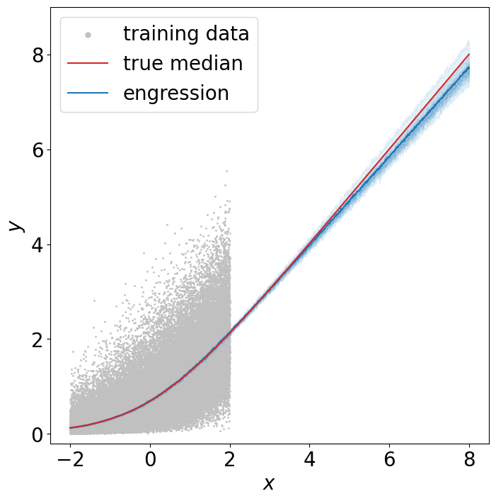
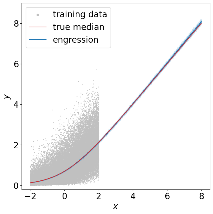
Conditional mean

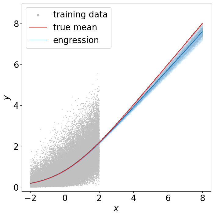
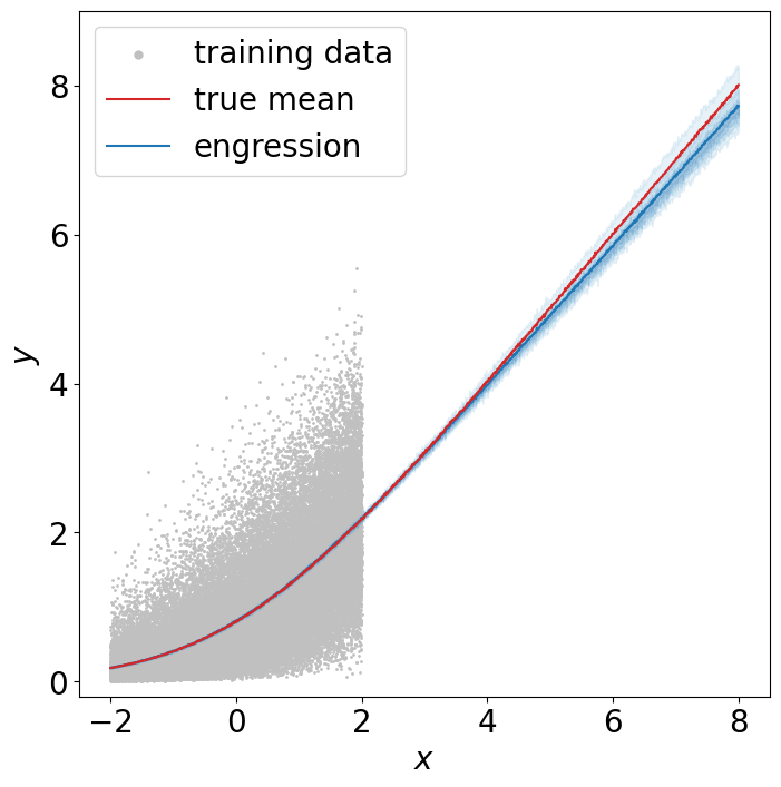
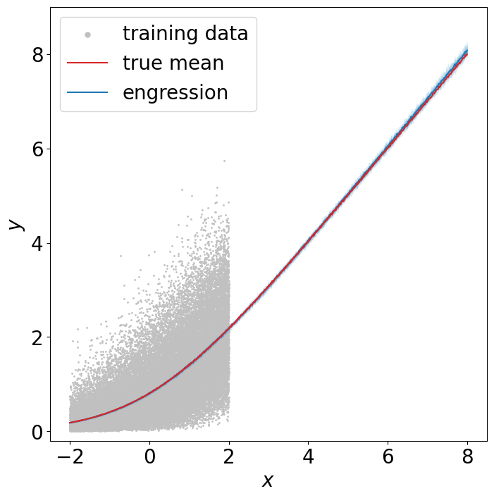
Figure 13: Performance of engression with other loss functions on softplus.

	Gaussian kernel	Laplace kernel	Inverse multiquadric kernel	KL GAN
Conditional median
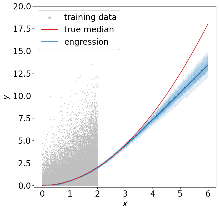
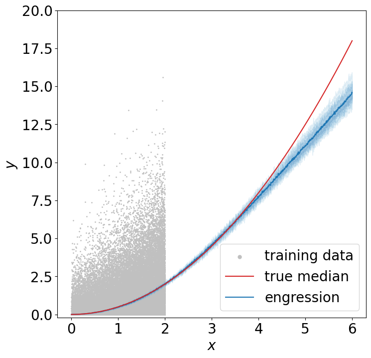
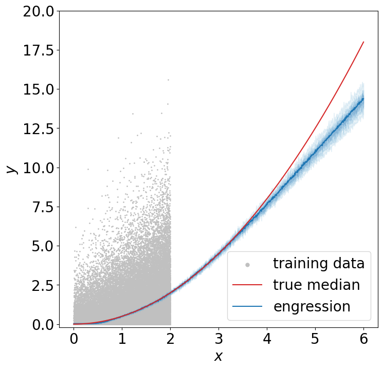
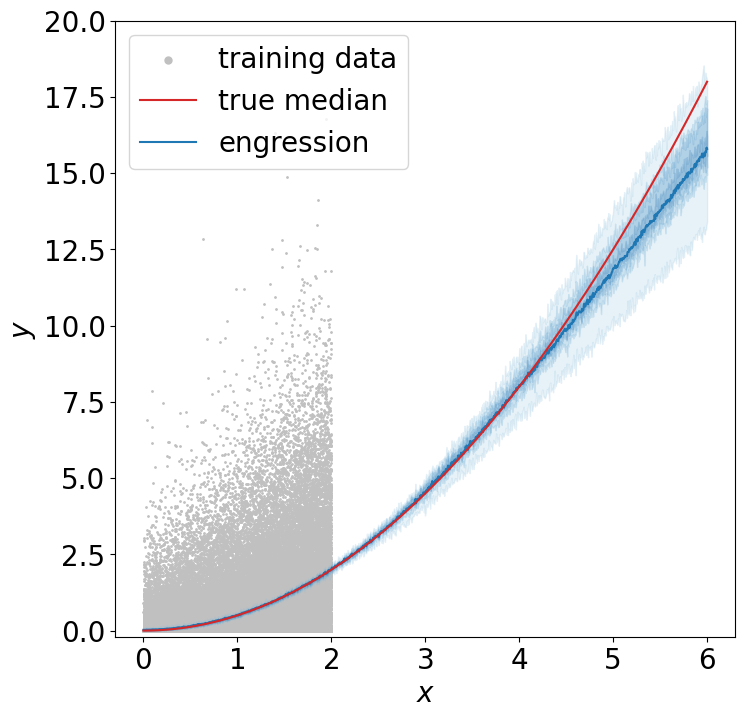
Conditional mean

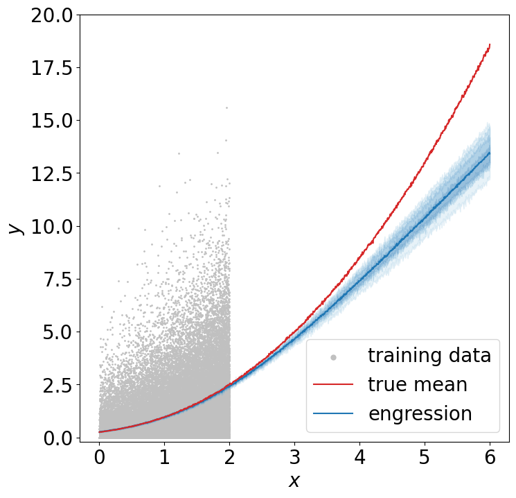
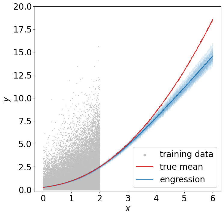
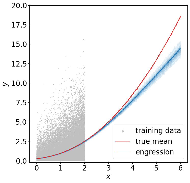
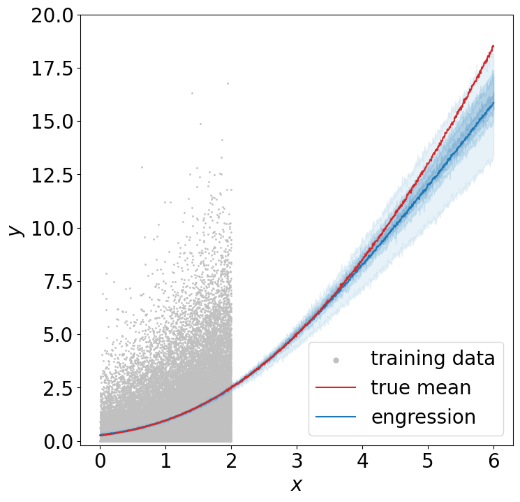
Figure 14: Performance of engression with other loss functions on square.

	Gaussian	Laplace	Inverse multiquadric	KL GAN
Conditional median
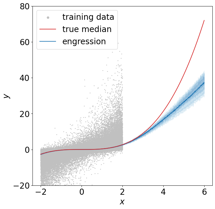
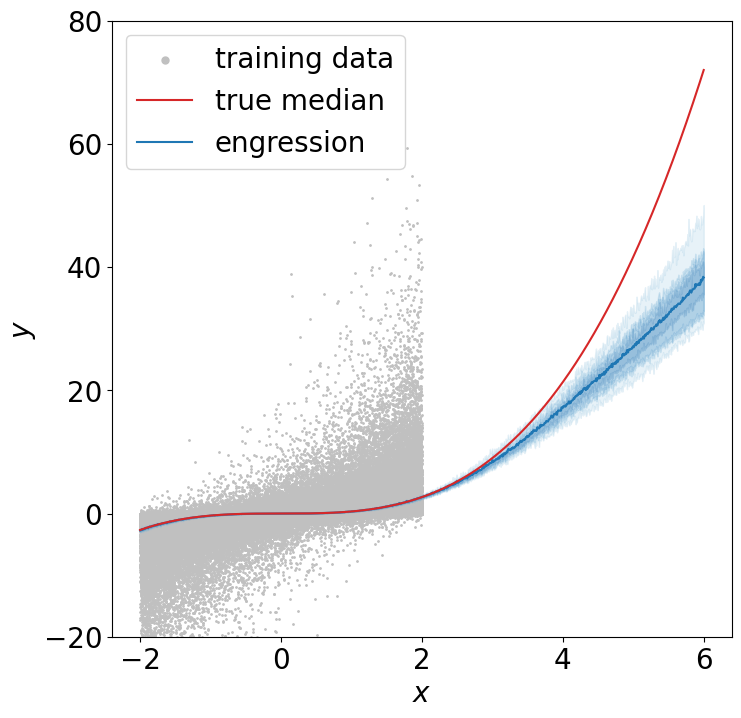
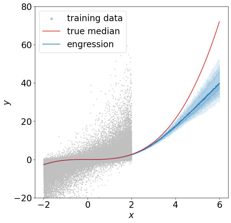
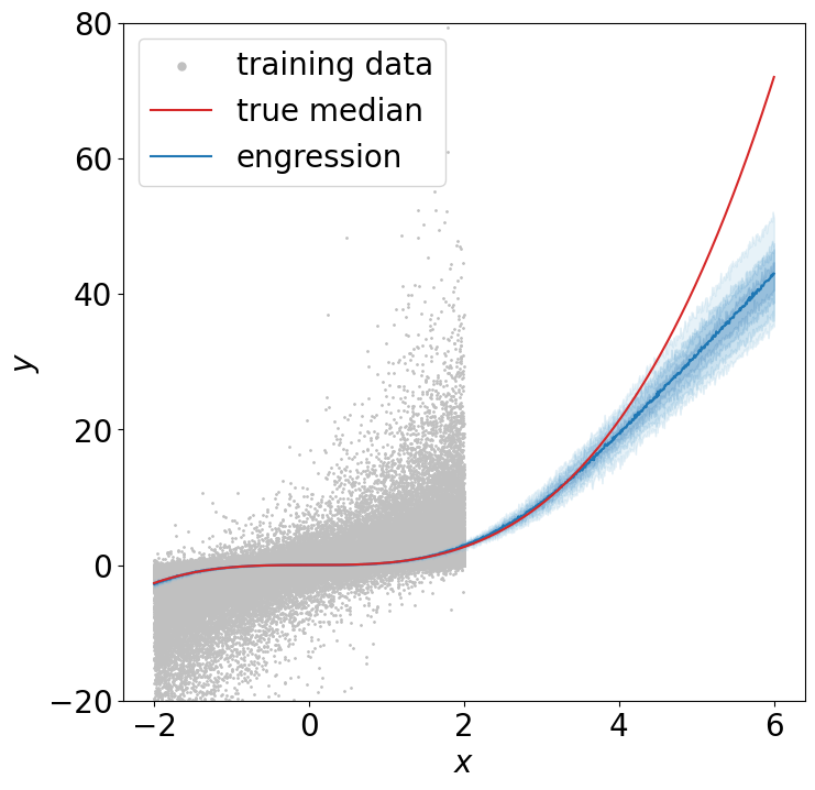
Conditional mean

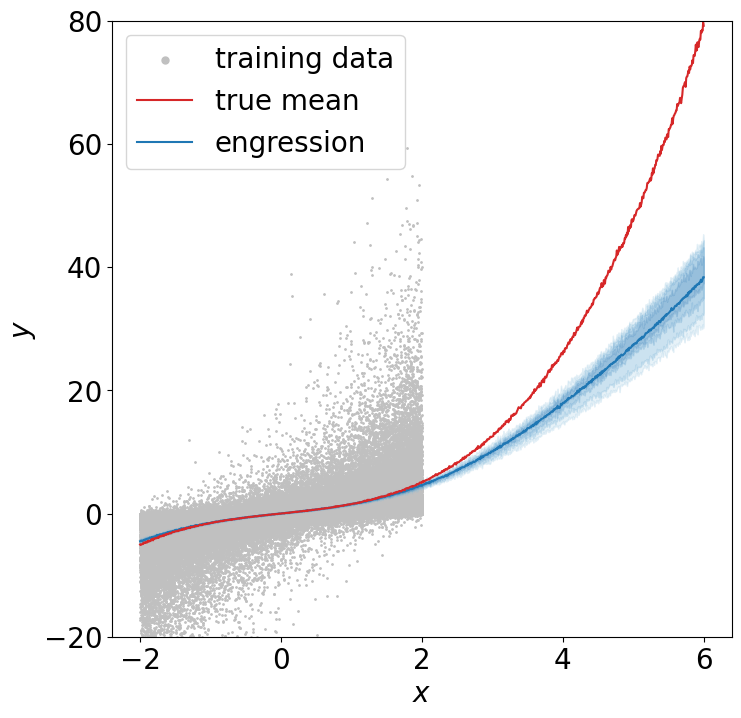
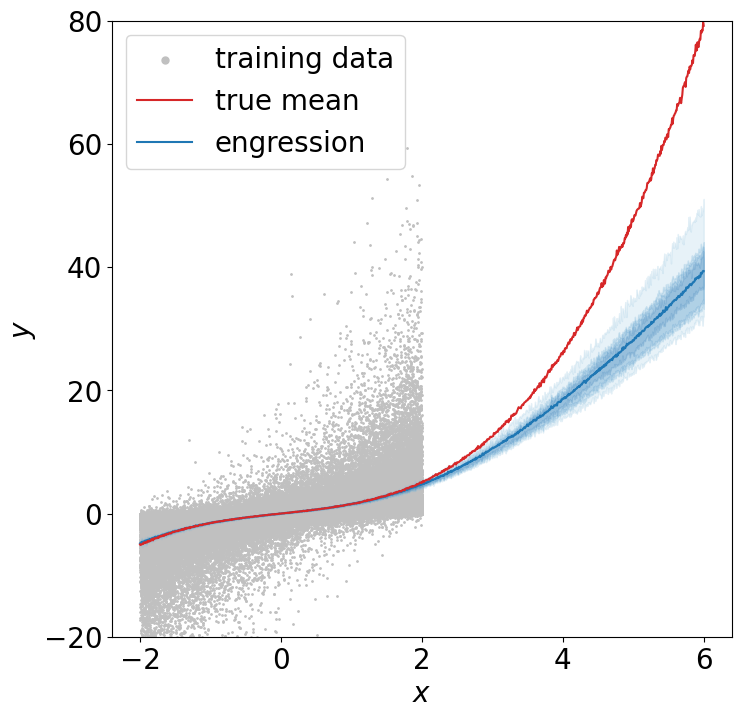
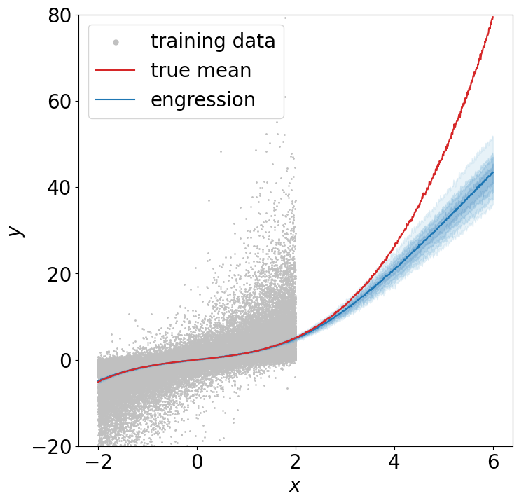
Figure 15: Performance of engression with other loss functions on cubic.

	Gaussian	Laplace	Inverse multiquadric	KL GAN
Conditional median
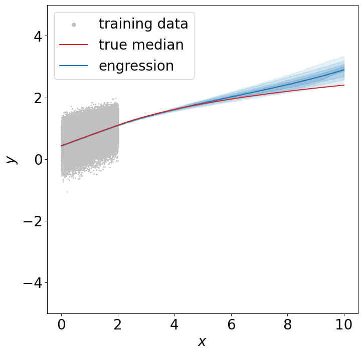
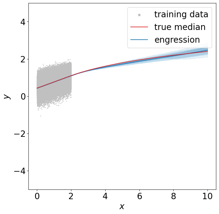
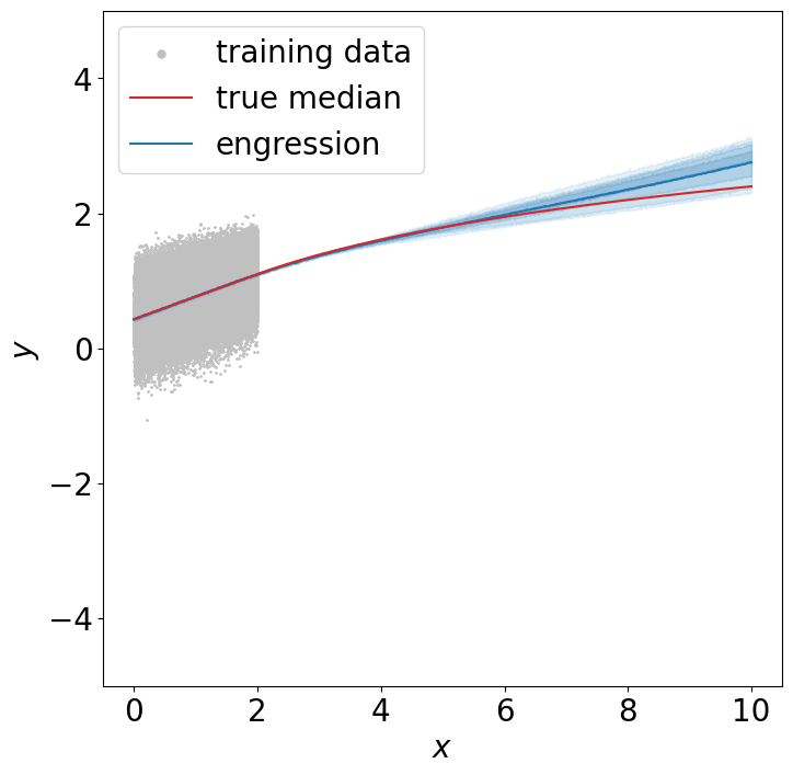
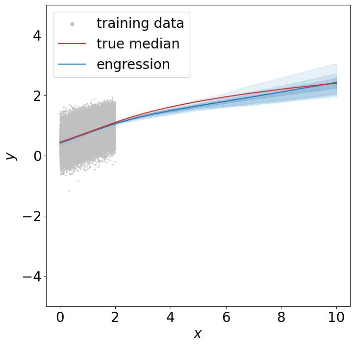
Conditional mean

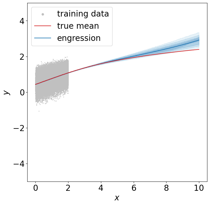
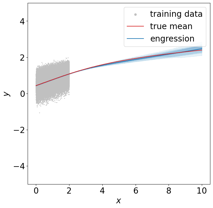
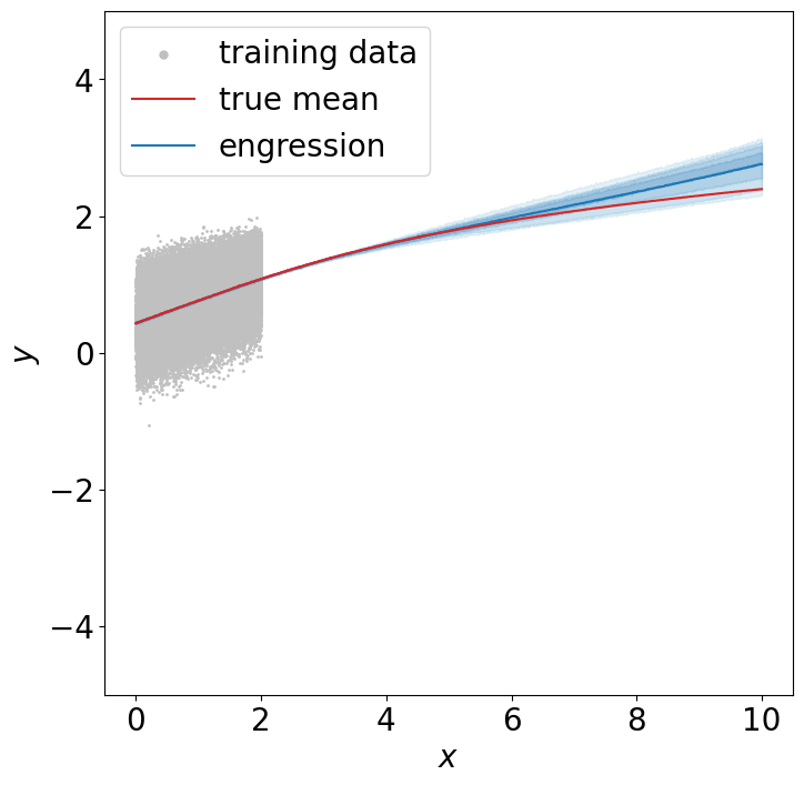
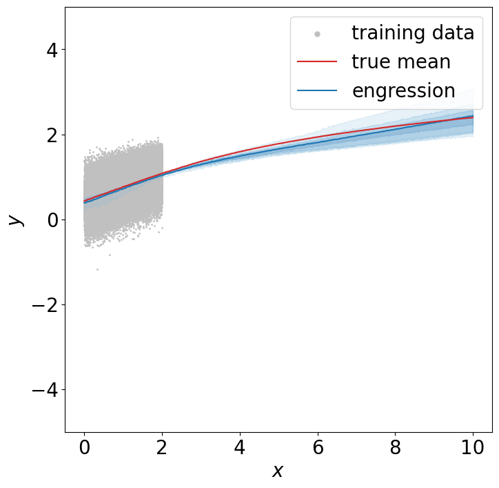
Figure 16: Performance of engression with other loss functions on log.

Appendix E Experimental details

We first describe the setup that we adopt generally across all experiments. For estimating the energy loss, at each gradient descent step, we use two generated samples for each observation of the covariate. We generate new samples of $\varepsilon$ for different steps, leading to a large generated sample size $m$ in total in the empirical loss in (10). Regarding the neural network architecture, we always adopt multilayer perceptrons (MLPs). In Figure 17, we illustrate the structure for one layer that we typically adopt for all input and intermediate layers (if the NN contains more than two layers); the output layer is always a single dense (fully-connected) layer. For $L_{1}$ and $L_{2}$ regression, we use deterministic networks, where each layer follows the same architecture in Figure 17 without concatenating any noise. For optimisation, we adopt the Adam optimiser (Kingma and Ba,, 2015) with default values for the beta parameters on the full batch of data in the experiments reported in this paper, while mini-batch gradient descent is implemented as well in our software. Throughout all experiments, we always keep the same NN architecture and optimisation hyperparameter for engression and regression. For engression, we typically set the noise dimension to $d_{n}=100$ unless stated otherwise.

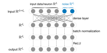
Figure 17: Architecture for one layer with input dimension $d_{i}$, noise dimension $d_{n}$ and output dimension $d_{o}$.

E.1 Simulations

For softplus and square, we simulate 50k training data and use NNs with one layer and 100 hidden neurons (i.e. one input layer as shown in Figure 17 followed by a dense output layer). For cubic and log, we simulate 100k training data and use NNs with 3 layers and 100 hidden neurons each. We adopt the Adam optimiser with a learning rate of $5\times 10^{-2}$ and train all the models for 10k iterations.

For kernel losses, we use exactly the same training setups as with the energy loss. For GAN, for numerical stability, we use a learning rate $1\times 10^{-3}$ for the model (generator) parameter $\theta$; at each gradient step of the pre-ANM, the discriminator is updated for 10 steps using the Adam optimiser with a learning rate of $5\times 10^{-3}$. The discriminator is an MLP with exactly the same architecture as the generator except no noise. All models are trained on the full batch for 10k iterations.

E.2 Real data

E.2.1 Data sets and preprocessing

We adopt 6 real, public data sets from various domains:

• GCM The GCM data set consists of 13,590 observations for three variables: daily global mean temperature (in Kelvin) obtained from the CanESM2 global circulation climate (GCM) model (Kushner et al.,, 2018) that covers the years 1950-2100 and regridded to a regular 2.5 degree-grid, the global annual mean radiation anomaly (in $W/m^{2}$) that summarises the Earth’s energy imbalance (e.g. from changing CO₂ concentrations), and the time stamp (integer). We consider predicting the temperature with either the radiation or time and the reverse direction.

• Abrupt4x The Abrupt4x data set contains temperature data from the CESM2 global circulation climate model (Danabasoglu et al.,, 2020) that spans 999 years. At the beginning, the CO₂ concentration in the atmosphere is multiplied by a factor of 4 compared to a pre-industrial level and then the climate slowly adjusts to a new and warmer equilibrium afterwards. We take the global mean temperature either monthly (using all years) or daily (using the first 209 years due to the huge sample size). We use the time stamp to predict either the monthly or daily temperature and predict the time using the temperatures.

• NHANES National Health and Nutrition Examination Survey (NHANES) is a nationally representative study conducted by the US Centers for Disease Control and Prevention (CDC) to assess the health and nutritional status of the United States population. In total, there were 20,470 study participants who participated in the NHANES 2003-2006 study. The original data set is obtained from the R package rnhanesdata (Leroux et al.,, 2019) and processed following a similar pipeline as described in Cui et al., (2021). For this experiment, we exclude participants who did not wear a physical activity monitor or had high-quality accelerometry data for less than 3 days and with missing BMI and age information. The final data set contains 10,914 participants. We focus on 4 variables: the total activity count (a unit measuring physical activity intensity), sedentary time (in minutes), body mass index, and age (in months). We do pairwise prediction for all pairs of variables in both directions.

• Single-cell The single-cell RNA sequencing data set was published by Replogle et al., (2022) who performed genome-scale Perturb-seq targeting all expressed genes with CRISPR perturbations across human cells. We utilise the data set on the RPE1 cells. After removing missing data and excluding genes with low expression, we select 6 pairs of genes with the highest correlation coefficient, with a sample size of around 11,400 for each pair. We do pairwise predictions in both directions.

• Birth This data set is obtained from the CDC Vital Statistics Data Online Portal (https://www.cdc.gov/nchs/data_access/vitalstatsonline.htm) and contains the information about around 3.8 million births in 2018, from which we remove all missing entries and randomly sample 30,000 individuals for our experiment. We focus on predicting the birth weight (in grams) from the pregnancy duration (in months, discrete).

• Air The air quality data set (Vito,, 2016) is obtained from the UCI machine learning repository. It contains hourly averaged concentrations for five pollutants: CO, Non Metanic HydroCarbons concentration (NMHC), Total Nitrogen Oxides (NOx), Nitrogen Dioxide (NO2), O3, and three meteorological covariates: temperature in degrees Celsius, relative humidity (in percentage) and absolute humidity (AH) for 8991 hours after removing missing values. We do pairwise predictions for all five pollutants, as well as NO2 – temperature, NO2 – AH, and AH – temperature in both directions.

In the large-scale experiments for univariate prediction, as described in Section 5.2.1, for each prediction task (i.e. a specific pair of the response and predictor), we partition the training and test data at the 0.3, 0.4, 0.5, 0.6, and 0.7 quantiles of the predictor and designate the smaller or larger portion as the training set. In Figure 18, we demonstrate one example of data setup on the air quality data. After training/test partitioning, we normalize the full data set based on the sample mean and standard deviation of the training set.

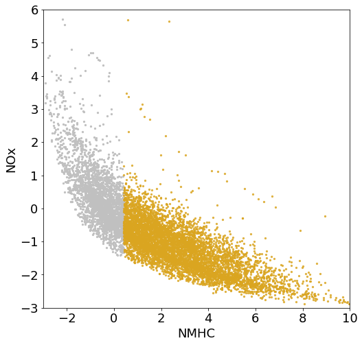
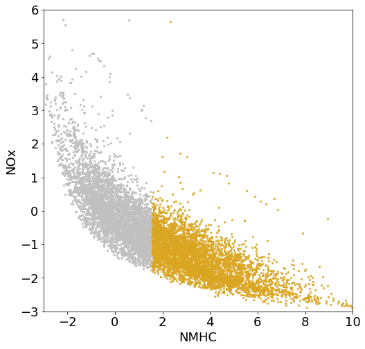
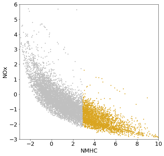
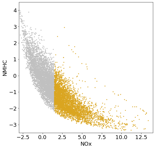
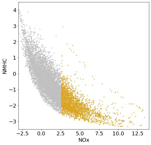
(a) 0.3	(b) 0.5	(c) 0.7	(d) flipped 0.3	(e) flipped 0.5	(f) flipped 0.7

Figure 18: An example of data setup on the air quality data. Partitioning training and test data at different quantiles of the predictor results in different levels of “similarity” between training and test distribution, implying varying difficulty for extrapolation. Comparing (d)-(e) to (a)-(c), flipping the roles of the predictor and response leads to potentially different underlying models.

E.2.2 Hyperparameters

For large-scale experiments on univariate prediction in Section 5.2.1, we consider various combinations of learning rates, numbers of training iterations, layers, and neurons per layer, as listed in Table 3.

For multivariate prediction in Section 5.2.2, we use exactly the same NN architectures and optimisation hyperparameters for both engression and regression and on both the air quality and NHANES data sets with any variables as the response. We use MLPs with 3 layers and 500 neurons per layer; for engression the noise dimension is set to 500 as well. We again use the Adam optimiser with a learning rate of 0.001 and train all models for 3000 iterations. For evaluation, the predictions for the conditional mean by engression are obtained by sampling 128 $\varepsilon$’s for each $x$, which is used for both visualisation and computing the squared prediction error.

For prediction intervals in Section 5.2.3, we again keep all the hyperparameters the same for engression and regression. For GCM data, we predict the global mean temperature from the time whose relationship is relatively simple, so we use an MLP with 2 layers and 100 hidden neurons trained for 500 iterations. For the air quality and NHANES data sets where the dependence is more complex, we use MLPs with 3 layers and 100 neurons per layer trained for 1000 iterations. The noise dimension for engression is 100 as typical. The Adam optimiser is adopted with a learning rate of 0.01.

Table 3: Set of hyperparameters. We experiment with all possible (in total 18) combinations.

(num_layer, hidden_dim)	(2, 100), (3, 10), (3, 100)
learning rate	$1\times 10^{-3}$, $1\times 10^{-2}$
number of training steps	500, 1000, 3000

References

- Arjovsky et al., (2019) Arjovsky, M., Bottou, L., Gulrajani, I., and Lopez-Paz, D. (2019). Invariant risk minimization. arXiv preprint arXiv:1907.02893.
- Arjovsky et al., (2017) Arjovsky, M., Chintala, S., and Bottou, L. (2017). Wasserstein generative adversarial networks. In Precup, D. and Teh, Y. W., editors, Proceedings of the 34th International Conference on Machine Learning, volume 70 of Proceedings of Machine Learning Research, pages 214–223. PMLR.
- Baringhaus and Franz, (2004) Baringhaus, L. and Franz, C. (2004). On a new multivariate two-sample test. Journal of Multivariate Analysis, 88(1):190–206.
- Bellemare et al., (2017) Bellemare, M. G., Danihelka, I., Dabney, W., Mohamed, S., Lakshminarayanan, B., Hoyer, S., and Munos, R. (2017). The cramer distance as a solution to biased wasserstein gradients. arXiv preprint arXiv:1705.10743.
- Ben-David et al., (2006) Ben-David, S., Blitzer, J., Crammer, K., and Pereira, F. (2006). Analysis of representations for domain adaptation. In Advances in Neural Information Processing Systems, volume 19.
- Breiman, (2001) Breiman, L. (2001). Random forests. Machine learning, 45:5–32.
- Brillinger, (2012) Brillinger, D. R. (2012). A generalized linear model with “gaussian” regressor variables. Selected Works of David Brillinger, pages 589–606.
- Bühlmann and Hothorn, (2007) Bühlmann, P. and Hothorn, T. (2007). Boosting Algorithms: Regularization, Prediction and Model Fitting. Statistical Science, 22(4):477 – 505.
- Bühlmann and Yu, (2003) Bühlmann, P. and Yu, B. (2003). Boosting with the l2 loss: regression and classification. Journal of the American Statistical Association, 98(462):324–339.
- Cauchy, (1847) Cauchy, A. (1847). Méthode générale pour la résolution des systemes d’équations simultanées. Comp. Rend. Sci. Paris, 25(1847):536–538.
- Chen and Bühlmann, (2021) Chen, Y. and Bühlmann, P. (2021). Domain adaptation under structural causal models. The Journal of Machine Learning Research, 22(1):11856–11935.
- Christiansen et al., (2021) Christiansen, R., Pfister, N., Jakobsen, M. E., Gnecco, N., and Peters, J. (2021). A causal framework for distribution generalization. IEEE Transactions on Pattern Analysis and Machine Intelligence, 44(10):6614–6630.
- Cui et al., (2021) Cui, E., Crainiceanu, C. M., and Leroux, A. (2021). Additive functional cox model. Journal of Computational and Graphical Statistics, 30(3):780–793.
- Danabasoglu et al., (2020) Danabasoglu, G., Lamarque, J.-F., Bacmeister, J., Bailey, D., DuVivier, A., Edwards, J., Emmons, L., Fasullo, J., Garcia, R., Gettelman, A., et al. (2020). The community earth system model version 2 (cesm2). Journal of Advances in Modeling Earth Systems, 12(2):e2019MS001916.
- Dawid, (2007) Dawid, A. P. (2007). The geometry of proper scoring rules. Annals of the Institute of Statistical Mathematics, 59:77–93.
- Dong and Ma, (2023) Dong, K. and Ma, T. (2023). First steps toward understanding the extrapolation of nonlinear models to unseen domains. In The Eleventh International Conference on Learning Representations.
- Dunson et al., (2007) Dunson, D. B., Pillai, N., and Park, J.-H. (2007). Bayesian density regression. Journal of the Royal Statistical Society Series B: Statistical Methodology, 69(2):163–183.
- Foresi and Peracchi, (1995) Foresi, S. and Peracchi, F. (1995). The conditional distribution of excess returns: An empirical analysis. Journal of the American Statistical Association, 90(430):451–466.
- Friedman, (2001) Friedman, J. H. (2001). Greedy function approximation: a gradient boosting machine. Annals of statistics, pages 1189–1232.
- Ganin and Lempitsky, (2015) Ganin, Y. and Lempitsky, V. (2015). Unsupervised domain adaptation by backpropagation. In Bach, F. and Blei, D., editors, Proceedings of the 32nd International Conference on Machine Learning, volume 37 of Proceedings of Machine Learning Research, pages 1180–1189, Lille, France. PMLR.
- Gneiting and Raftery, (2007) Gneiting, T. and Raftery, A. E. (2007). Strictly proper scoring rules, prediction, and estimation. Journal of the American statistical Association, 102(477):359–378.
- Goodfellow et al., (2014) Goodfellow, I., Pouget-Abadie, J., Mirza, M., Xu, B., Warde-Farley, D., Ozair, S., Courville, A., and Bengio, Y. (2014). Generative adversarial nets. In Ghahramani, Z., Welling, M., Cortes, C., Lawrence, N., and Weinberger, K., editors, Advances in Neural Information Processing Systems, volume 27. Curran Associates, Inc.
- Gretton et al., (2012) Gretton, A., Borgwardt, K. M., Rasch, M. J., Schölkopf, B., and Smola, A. (2012). A kernel two-sample test. The Journal of Machine Learning Research, 13(1):723–773.
- Gretton et al., (2009) Gretton, A., Smola, A., Huang, J., Schmittfull, M., Borgwardt, K., and Schölkopf, B. (2009). Covariate shift by kernel mean matching. Dataset shift in machine learning, 3(4):5.
- Gulrajani et al., (2017) Gulrajani, I., Ahmed, F., Arjovsky, M., Dumoulin, V., and Courville, A. C. (2017). Improved training of wasserstein gans. In Advances in Neural Information Processing Systems, volume 30.
- Hardle et al., (1993) Hardle, W., Hall, P., and Ichimura, H. (1993). Optimal smoothing in single-index models. The annals of Statistics, 21(1):157–178.
- Hothorn et al., (2014) Hothorn, T., Kneib, T., and Bühlmann, P. (2014). Conditional transformation models. Journal of the Royal Statistical Society: Series B: Statistical Methodology, pages 3–27.
- Kingma and Ba, (2015) Kingma, D. P. and Ba, J. (2015). Adam: A method for stochastic optimization. In Proceedings of the 3rd International Conference on Learning Representations (ICLR).
- Kneib et al., (2023) Kneib, T., Silbersdorff, A., and Säfken, B. (2023). Rage Against the Mean – A Review of Distributional Regression Approaches. Econometrics and Statistics, 26(C):99–123.
- Koenker, (2005) Koenker, R. (2005). Quantile regression, volume 38. Cambridge university press.
- Koenker and Bassett, (1978) Koenker, R. and Bassett, G. (1978). Regression quantiles. Econometrica: journal of the Econometric Society, pages 33–50.
- Kushner et al., (2018) Kushner, P. J., Mudryk, L. R., Merryfield, W., Ambadan, J. T., Berg, A., Bichet, A., Brown, R., Derksen, C., Déry, S. J., Dirkson, A., et al. (2018). Canadian snow and sea ice: assessment of snow, sea ice, and related climate processes in canada’s earth system model and climate-prediction system. The Cryosphere, 12(4):1137–1156.
- Legendre, (1806) Legendre, A. M. (1806). Nouvelles méthodes pour la détermination des orbites des comètes; par AM Legendre… chez Firmin Didot, libraire pour lew mathematiques, la marine, l ….
- Lei et al., (2018) Lei, J., G’Sell, M., Rinaldo, A., Tibshirani, R. J., and Wasserman, L. (2018). Distribution-free predictive inference for regression. Journal of the American Statistical Association, 113(523):1094–1111.
- Leroux et al., (2019) Leroux, A., Di, J., Smirnova, E., Mcguffey, E. J., Cao, Q., Bayatmokhtari, E., Tabacu, L., Zipunnikov, V., Urbanek, J. K., and Crainiceanu, C. (2019). Organizing and analyzing the activity data in nhanes. Statistics in biosciences, 11:262–287.
- Massart, (1990) Massart, P. (1990). The tight constant in the dvoretzky-kiefer-wolfowitz inequality. The annals of Probability, pages 1269–1283.
- Matheson and Winkler, (1976) Matheson, J. E. and Winkler, R. L. (1976). Scoring rules for continuous probability distributions. Management science, 22(10):1087–1096.
- McCullagh and Nelder, (1983) McCullagh, P. and Nelder, J. (1983). Generalized Linear Models. Monographs on Statistics and Applied Probability. Springer US.
- Meinshausen, (2006) Meinshausen, N. (2006). Quantile regression forests. Journal of machine learning research, 7(6).
- Mirza and Osindero, (2014) Mirza, M. and Osindero, S. (2014). Conditional generative adversarial nets. arXiv preprint arXiv:1411.1784.
- Nowozin et al., (2016) Nowozin, S., Cseke, B., and Tomioka, R. (2016). f-gan: Training generative neural samplers using variational divergence minimization. In Advances in Neural Information Processing Systems, volume 29.
- Peters et al., (2016) Peters, J., Bühlmann, P., and Meinshausen, N. (2016). Causal inference by using invariant prediction: identification and confidence intervals. Journal of the Royal Statistical Society. Series B (Statistical Methodology), pages 947–1012.
- Replogle et al., (2022) Replogle, J. M., Saunders, R. A., Pogson, A. N., Hussmann, J. A., Lenail, A., Guna, A., Mascibroda, L., Wagner, E. J., Adelman, K., Lithwick-Yanai, G., et al. (2022). Mapping information-rich genotype-phenotype landscapes with genome-scale perturb-seq. Cell, 185(14):2559–2575.
- Robbins and Monro, (1951) Robbins, H. and Monro, S. (1951). A stochastic approximation method. The annals of mathematical statistics, pages 400–407.
- Rothenhäusler et al., (2021) Rothenhäusler, D., Meinshausen, N., Bühlmann, P., and Peters, J. (2021). Anchor regression: Heterogeneous data meet causality. Journal of the Royal Statistical Society Series B: Statistical Methodology, 83(2):215–246.
- Sejdinovic et al., (2013) Sejdinovic, D., Sriperumbudur, B., Gretton, A., and Fukumizu, K. (2013). Equivalence of distance-based and rkhs-based statistics in hypothesis testing. The annals of statistics, pages 2263–2291.
- Shafer and Vovk, (2008) Shafer, G. and Vovk, V. (2008). A tutorial on conformal prediction. Journal of Machine Learning Research, 9(3).
- Shen et al., (2022) Shen, X., Chen, K., and Zhang, T. (2022). Asymptotic statistical analysis of -divergence gan. arXiv preprint arXiv:2209.06853.
- Steinwart and Ziegel, (2021) Steinwart, I. and Ziegel, J. F. (2021). Strictly proper kernel scores and characteristic kernels on compact spaces. Applied and Computational Harmonic Analysis, 51:510–542.
- Sugiyama et al., (2007) Sugiyama, M., Krauledat, M., and Müller, K.-R. (2007). Covariate shift adaptation by importance weighted cross validation. Journal of Machine Learning Research, 8(5).
- Székely, (2003) Székely, G. J. (2003). E-statistics: The energy of statistical samples. Bowling Green State University, Department of Mathematics and Statistics Technical Report, 3(05):1–18.
- Székely and Rizzo, (2023) Székely, G. J. and Rizzo, M. L. (2023). The Energy of Data and Distance Correlation. CRC Press.
- Taleb and Jutten, (1999) Taleb, A. and Jutten, C. (1999). Source separation in post-nonlinear mixtures. IEEE Transactions on signal Processing, 47(10):2807–2820.
- Vito, (2016) Vito, S. (2016). Air Quality. UCI Machine Learning Repository. DOI: https://doi.org/10.24432/C59K5F.
- Zhang and Hyvärinen, (2009) Zhang, K. and Hyvärinen, A. (2009). On the identifiability of the post-nonlinear causal model. In Conference on Uncertainty in Artificial Intelligence.