Anisotropic Fanning Aware Low-Rank Tensor Approximation Based Tractography

Abstract

Low-rank higher-order tensor approximation has been used successfully to extract discrete directions for tractography from continuous fiber orientation density functions (fODFs). However, while it accounts for fiber crossings, it has so far ignored fanning, which has led to incomplete reconstructions. In this work, we integrate an anisotropic model of fanning based on the Bingham distribution into a recently proposed tractography method that performs low-rank approximation with an Unscented Kalman Filter. Our technical contributions include an initialization scheme for the new parameters, which is based on the Hessian of the low-rank approximation, pre-integration of the required convolution integrals to reduce the computational effort, and representation of the required 3D rotations with quaternions. Results on 12 subjects from the Human Connectome Project confirm that, in almost all considered tracts, our extended model significantly increases completeness of the reconstruction, while reducing excess, at acceptable additional computational cost. Its results are also more accurate than those from a simpler, isotropic fanning model that is based on Watson distributions.

1 Introduction

Diffusion MRI tractography [11] permits the in-vivo reconstruction of white matter tracts in surgery planning or scientific studies. Spherical deconvolution is widely used to account for intra-voxel heterogeneity by estimating a continuous fiber orientation density function (fODF) in each voxel [7]. Representing fODFs as higher-order tensors and applying a low-rank approximation to these tensors has been shown to be a robust and efficient approach to estimating discrete tracking directions [20, 1].

However, while low-rank approximation accounts for fiber crossings, it ignores fiber fanning [21]. Consequently, even though recent work [9] has achieved promising results by performing low-rank approximation within the framework of Unscented Kalman Filter (UKF) based tractography [17], some fanning bundles were extracted incompletely when using single-region seeding strategies [9].

We address this limitation by explicitly modeling anisotropic fanning in the low-rank UKF with Bingham distributions [13]. This involves three main technical challenges: Firstly, initializing additional parameters in the UKF state. Section 3.2 solves this by observing that the Hessian matrix at the optimum of the low-rank approximation indicates the amount and direction of fanning. Secondly, the computational effort of convolving rank-one tensors with Bingham distributions. Section 3.3 solves this by pre-computing the corresponding integrals and storing results in lookup tables. Thirdly, maintaining a full 3D rotation per fiber compartment. Section 3.4 solves this with a quaternion-based representation. Results in Section 4 indicate that our extension reconstructs fanning bundles significantly more completely, while reducing excess, at acceptable additional computational cost.

2 Background and Related Work

2.1 Low-rank tensor approximation model

Constrained spherical deconvolution (CSD) computes the fiber orientation distribution function (fODF), a mapping from the sphere to $\mathbb{R}_{+}$ which captures the fraction of fibers in any direction [22]. One widely used strategy for estimating principal fiber orientations is to consider local fODF maxima. Our work builds on a variation of CSD, which represents the fODF as a symmetric higher-order tensor $\mathcal{T}$ and estimates $r$ fiber directions via a rank-$r$ approximation

$$\mathcal{T}^{\left(r\right)}=\sum_{i=1}^{r}\alpha_{i}\mathbf{v}_{i}^{\otimes l},$$ (1)

where the scalar $\alpha_{i}\in\mathbb{R}_{+}$ denotes the volume fraction of the $i$th fiber, $\mathbf{v}_{i}\in\mathbb{S}^{2}$ its direction, and the superscript $\otimes l$ indicates an $l$-fold symmetric outer product, which turns the vector into an order-$l$ tensor. The main benefit of this approach is that it can separate crossing fibers even if they are not distinct local maxima, which permits the use of lower orders and in turn improves numerical conditioning and computational effort [1]. Specifically, the angular resolution of fourth-order tensor approximation for crossing fibers has been shown to exceed order-eight fODFs with peak extraction [1]. To additionally capture information about anisotropic fanning, our current work increases the tensor order to $l=6$, which parameterizes each fODF with 28 degrees of freedom.

2.2 Bingham distribution

The Bingham distribution [3] is the spherical and antipodally symmetric $(f\left(\mathbf{x}\right)=f\left(-\mathbf{x}\right))$ analogue to a two dimensional Gaussian distribution. It is given by the probability density function

$$f\left(\mathbf{x};\mathbf{M},\mathbf{Z}\right)\coloneqq\frac{1}{N\left(\mathbf{Z}\right)}\exp\left(\mathbf{x}^{T}\mathbf{M}\mathbf{Z}\mathbf{M}^{T}\mathbf{x}\right),$$ (2)

where $\mathbf{Z}$ is a diagonal matrix with decreasing entries $z_{1}\geq z_{2}\geq z_{3}$, $\mathbf{M}=\left(\mu_{1},\mu_{2},\mu_{3}\right)$ is an orthogonal matrix and $N\left(\mathbf{Z}\right)$ denotes the hypergeometric function of matrix argument. Without loss of generality, we set $z_{3}=0$ and rename $\kappa=z_{1},\beta=z_{2}$ to rewrite the density function as:

$$f\left(\mathbf{x};\mu_{1},\mu_{2},\kappa,\beta\right)=\frac{1}{N\left(\kappa,\beta\right)}\exp\left(\kappa\langle\mu_{1},\mathbf{x}\rangle^{2}+\beta\langle\mu_{2},\mathbf{x}\rangle^{2}\right).$$ (3)

The Bingham distribution was used previously to model anisotropic fanning: Riffert et al. [18] fitted a mixture of Bingham distributions to the fODF to compute metrics such as peak spread and integral over peak. Kaden et al. [13] used it for Bayesian tractography. Our contribution combines the Bingham distribution with the low-rank model, and estimates the resulting parameters with a computationally efficient Unscented Kalman Filter.

2.3 Unscented Kalman Filter

The Kalman Filter is an algorithm that estimates a set of unknown variables, typically referered to as the state, from a series of noisy observations over time. The Unscented Kalman Filter (UKF) [12] is an extension that permits a non-linear relationship between the unknown variables and the measurements. It has first been used for tractography by Malcolm et al. [16, 17], who treat the diffusion MR signal as consecutive measurements along a fiber, and the parameters of a mixture of diffusion tensors [16] or Watson distributions [17] as the unknown variables. Compared to independent estimation of model parameters at each location, this approach reduces the effects of measurement noise by combining local information with the history of previously encountered values. Consequently, it has been used for scientific studies [4, 6] as well as neurosurgical planning [5].

Recent work has used the UKF to estimate the parameters of the low-rank model [9]. This variant of the UKF treats the fODFs instead of the raw diffusion MR signal as its measurements, which increases tracking accuracy while reducing computational cost, due to the much lower number of fODF parameters compared to diffusion-weighted volumes. A remaining limitation of that approach is that it does not account for fanning.

3 Material and Methods

We extend the previously described low-rank UKF [9] by modeling directional fanning with a Bingham distribution (Section 3.1). Implementing this requires solving problems related to initialization (Section 3.2), efficient evaluation of certain integrals (Section 3.3), and representing rigid body orientations within the UKF (Section 3.4). Section 3.5 describes the resulting tractography algorithm, while Section 3.6 reports the data and measures that we use for evaluation.

3.1 Low-rank model with anisotropic fanning

The higher-order tensor variant of CSD adapts the deconvolution so that it maps the single fiber response to a rank-one tensor [20]. Therefore, fanning can be incorporated by convolving the rank-$1$ kernel $k$ with the Bingham distribution

$$h^{\left(r\right)}=\sum_{i=1}^{r}\alpha_{i}f\left(\cdot;\mu^{\left(i\right)}_{1},\mu^{\left(i\right)}_{2},\kappa^{\left(i\right)},\beta^{\left(i\right)}\right)\star k,$$ (4)

where $\alpha_{i}$ denotes the volume fraction of the $i$th fiber in direction $\mu^{\left(i\right)}_{1}$, $\kappa^{(i)}$ the concentration around it (i.e., the inverse to the amount of fanning). In case of anisotropic fanning, $\beta^{(i)}>0$ indicates the additional amount of fanning in direction $\mu^{\left(i\right)}_{2}$. For $\kappa^{(i)}\rightarrow\infty$ and $\beta^{(i)}=0$, the Bingham distributions converge to delta peaks and the model (4) converges towards the original low-rank model (1) with fiber directions $\mu^{\left(i\right)}_{1}=\mathbf{v}_{i}$.

3.2 Initialization via the low-rank model

Since it is difficult to fit the model in Eq. (4) to data, we initialize the UKF based on the original low-rank approximation in Eq. (1). Firstly, we use the same main fiber directions, $\mu^{\left(i\right)}_{1}=\mathbf{v}_{i}$. Secondly, we initialize the fanning related parameters by observing that the rate at which the approximation error grows when rotating a given fiber direction away from its optimum depends on the amount of fanning: The lower the amount of fanning (the sharper the fODF peak), the more sensitive is the approximation error to the exact direction.

For each fiber, this information is captured in the second derivatives of the cost function with respect to its orientation, i.e., a $2\times 2$ Hessian that can be computed in spherical coordinates; an equation for this is derived in [19]. There is a one-to-one mapping between the eigenvalues of that Hessian and corresponding values of $\kappa$ and $\beta$. The eigenvector corresponding to the lower eigenvalue indicates the dominant fanning direction $\mu_{2}$.

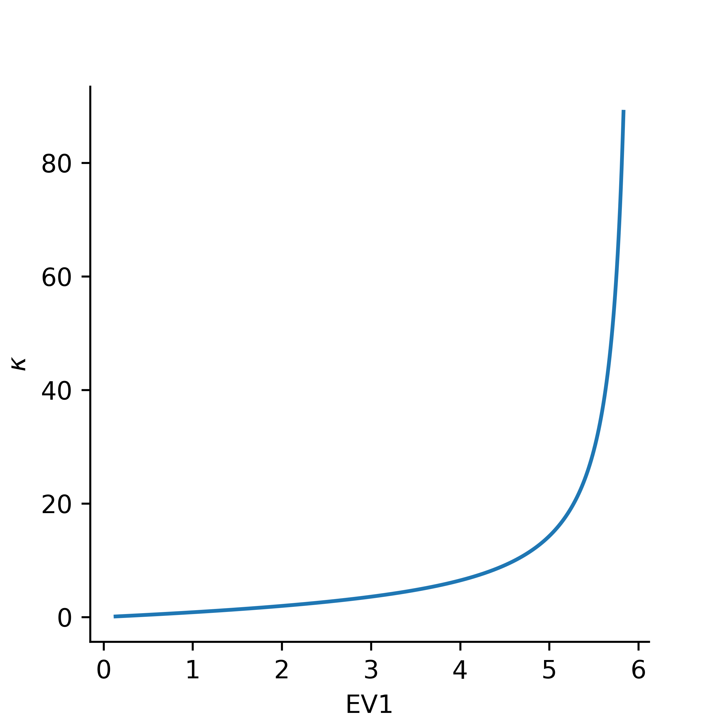
(a) Mapping from larger eigenvalue to $\kappa$

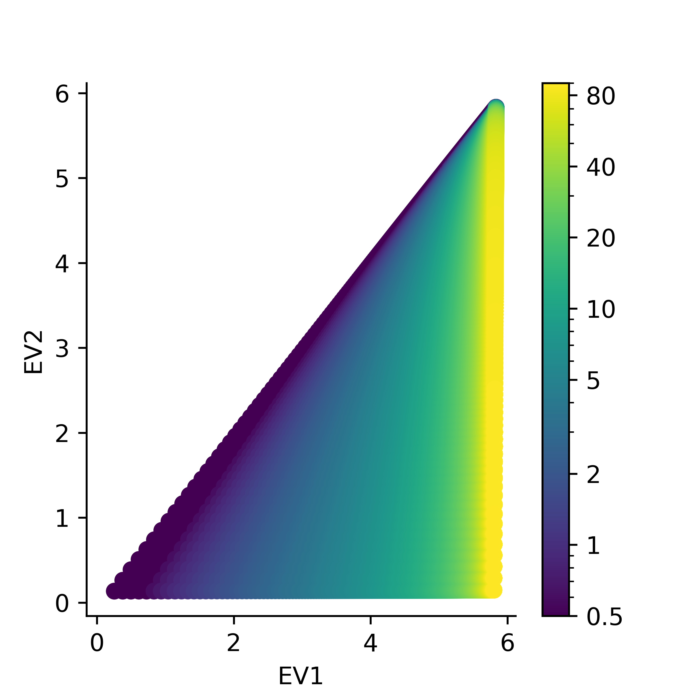
(b) Mapping from eigenvalues to $\beta$

Figure 1: Lookup tables for initializing $\kappa$ and $\beta$ based on Hessian eigenvalues. Left: $\kappa$ is fully determined by the larger eigenvalue. Right: $\beta=0$ if both eigenvalues are the same, but increases as EV2 decreases for a fixed value of EV1.

We pre-compute a lookup table for the values of $\kappa$ and $\beta$, given the Hessian eigenvalues. To this end, we utilize the model (4) to generate single fiber fODFs for various combinations of $\kappa$ and $\beta$ values, and record the resulting eigenvalues. Figure 1 visualizes the mapping from eigenvalues to $\kappa$ and $\beta$. Subfigure 1(a) shows that $\kappa$ increases with the larger eigenvalue, indicating a higher concentration around the main fiber direction. Subfigure 1(b) shows how $\beta$ depends on both eigenvalues. If they are the same, fanning is isotropic ($\beta=0$), while for any given larger eigenvalue (EV1), $\beta$ increases, indicating an increasingly elliptic fanning, as the smaller eigenvalues (EV2) decreases towards zero.

We apply this lookup table to multi-fiber voxels by computing the residual fODF for each fiber (i.e., we subtract out the remaining fibers), and normalizing it such that $\alpha=1$ to eliminate scaling effects. After fixing all fiber directions and fanning parameters, we fit the remaining volume fractions $\alpha_{i}$ in Eq. (4) with a non-negative least squares solver.

3.3 Pre-computing the convolution

Equation (4) involves a convolution between a rank-$1$ kernel and a Bingham distribution. To compute it efficiently, we first split the Bingham distribution into a standard version and a rotation part. We rewrite

$$f\left(\mathbf{x};\mathbf{M},\mathbf{Z}\right)=\left(D\left(\vartheta,\psi,\omega\right)g\right)\left(\mathbf{x};\kappa,\beta\right)=g\left(\mathbf{M}^{-1}\mathbf{x};\kappa,\beta\right),$$ (5)

where $g\left(\mathbf{x},\kappa,\beta\right)\coloneqq\frac{1}{N\left(\mathbf{Z}\right)}\exp\left(\kappa\mathbf{x}_{3}^{2}+\beta\mathbf{x}_{2}^{2}\right)$ is a standard Bingham distribution in the canonical basis oriented towards the north pole and $D$ is the $zyz$ rotation matrix, which is defined as

$$\mathbf{M}=D\left(\vartheta,\psi,\omega\right)\coloneqq R_{z}\left(\vartheta\right)R_{y}\left(\psi\right)R_{z}\left(\omega\right)$$ (6)

with

$$R_{z}\left(\alpha\right)\coloneqq\left(\begin{matrix}\cos\alpha&\sin\alpha&0\\ -\sin\alpha&\cos\alpha&0\\ 0&0&1\\ \end{matrix}\right)\text{ and }R_{y}\left(\alpha\right)\coloneqq\left(\begin{matrix}\cos\alpha&0&\sin\alpha\\ 0&1&0\\ -\sin\alpha&0&\cos\alpha\\ \end{matrix}\right).$$ (7)

This decomposition is a significant simplification, because we can now pre-compute the convolution between the standard Bingham distribution and the kernel, and apply the rotation afterwards.

As it is standard practice in CSD [22], we perform the convolution on the sphere using spherical and rotational harmonics. A rotational harmonics representation of the rank-1 kernel has been computed previously [20]. Unfortunately, no closed form solution is available for the spherical harmonics coefficients of the Bingham distribution. Therefore, we pre-compute them numerically, for the relevant range of $\kappa\in\left\{2.1,2.2,\dots,89\right\}$ and $\beta\in\left\{0,0.1,\dots,\kappa-2\right\}$.

3.4 Representing rotations with quaternions

Unlike previous UKF-based tractography methods, our model requires a full three-dimensional rotation per fiber to account not just for the fiber direction, but also for the direction of its anisotropic spread. Unit quaternions are a popular representation of rotations, since they overcome limitations of Euler angles, such as gimbal lock. However, integrating them into a UKF is non trivial, since their normalization leads to dependencies within the state [14]. We overcome the problem by utilizing a homeomorphism between quaternions and $\mathbb{R}^{3}$. We discuss the relevant steps of that approach, but refer the reader to work by Bernal-Polo et al. [2] for a more detailed discussion of quaternions and this way of integrating them into the UKF. More detailed explanations of UKF-based tractography are also available in the literature [16, 17, 9].

Given a quaternion $q=\left[q_{w},q_{x},q_{y},q_{z}\right]\in\mathbb{H}$, we define a homeomorphism

$$\phi:\mathbb{S}^{3} \rightarrow\left\{\mathbf{e}\in\mathbb{R}^{3}:\|\mathbf{e}\|\leq 4\right\}$$ (8)

$$q \mapsto 4\frac{q_{1:}}{1+q_{0}}$$ (9)

to the so-called Modified Rodrigues Parameters [26] and, vice versa,

$$\phi^{-1}:\left\{\mathbf{e}\in\mathbb{R}^{3}:\|\mathbf{e}\|\leq 4\right\} \rightarrow\mathbb{S}^{3}$$ (10)

$$\mathbf{e} \mapsto\frac{1}{16+\|\mathbf{e}\|^{2}}\left(16-\|\mathbf{e}\|^{2},8\mathbf{e}\right).$$ (11)

In a close neighborhood of the identity quaternion, these charts behave like the identity transformation between the imaginary part of quaternions and $\mathbb{R}^{3}$. For a given mean quaternion $\bar{q}$ of a quaternions set $\left\{q_{i}\right\}_{i}$, we define a mapping which first maps each $q_{i}$ by the conjugated mean quaternion, pushes it to $\mathbb{R}^{3}$,

$$\phi_{\bar{q}}\left(q_{i}\right)\coloneqq\phi\left(\bar{q}^{\star}\star q_{i}\right)=\mathbf{e},$$ (12)

where $\bar{q}^{\star}=\left[\bar{q}_{w},-\bar{q}_{x},-\bar{q}_{y},-\bar{q}_{z}\right]$ denotes the conjugated quaternion, pulls it back and rotates it back via

$$\phi^{-1}_{\bar{q}}\left(\mathbf{e}\right)\coloneqq\bar{q}\star\phi^{-1}\left(\mathbf{e}\right).$$ (13)

Assuming that the quaternions are highly concentrated around the mean quaternion, the embedding resembles the distribution of quaternions closely.

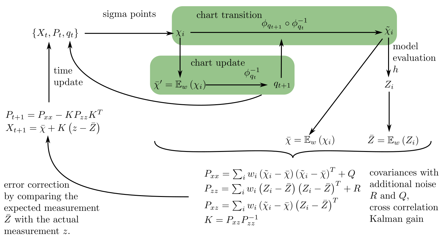
Figure 2: Schematic representation of an UKF update step. Compared to a normal UKF update, we additionally update the charts by first calculating the weighted mean of the sigma points and pulling it back into quaternion space. With the new quaternion, we perform a chart transition. The remaining steps are analogue to the traditional UKF.

With these preliminaries, we set up the UKF as illustrated in Figure 2. We only show it for a single fiber direction. For simplicity, our implementation updates the parameters for each fiber separately. The state at point $t$ is defined by the parameters of a single Bingham distribution in the embedded space

$$X_{t}\coloneqq\left\{\alpha,\kappa,\beta,\mathbf{e}_{1},\mathbf{e}_{2},\mathbf{e}_{3}\right\}.$$ (14)

The embedding is fully determined by the quaternion $q_{t}$ and the covariance is denoted by $P_{t}$.

We create sigma points to capture the distribution of the covariance around the current mean. We use the sigma points to calculate a chart update $q_{t+1}$, by taking a weighted mean with weights $w_{i}$ and pulling the embedded part back into quaternion space. With the new chart we perform a chart transition. Afterwards, we follow the standard UKF update scheme: Firstly, calculate the weighted mean of the sigma points, evaluate our model for all sigma points and take the corresponding weighted mean. Secondly, calculate the covariance $P_{xx}$ of the sigma points, the covariance of the evaluation $P_{zz}$ and the cross correlation $P_{xy}$. This information is then used to calculate the Kalman gain $K$ and correct the current state $X_{t}$ dependent on the difference between the expected measurement $\bar{Z}$ and the fODF $z$ as well as the covariance.

3.5 Probabilistic streamline-based tractography

For a given seed point, we initialize the UKF as discussed in Section 3.2. We perform streamline integration with second-order Runge-Kutta: At the $j$th point of the streamline, we update the UKF, select the Bingham distribution whose main direction is closest by angle to the current tracking direction, and draw a direction from that Bingham distribution via rejection sampling. We use that direction for a tentative half-step, again update the UKF and perform rejection sampling. Finally, we reach point $(j+1)$ by taking a full step from point $j$ in that new direction. This process is iteratively conducted until a stopping criterion is reached. We stop the integration if the white matter density drops below $0.4$ or if we cannot find any valid direction within 60 degrees.

3.6 Data and evaluation

It is the goal of our work to modify the UKF so that it more completely reconstructs fanning bundles from seeds in a single region. We evaluate this on 12 subjects from the Human Connectome Project (HCP) [23] for which reference tractographies have been published as part of TractSeg [25]. They are based on a segmented and manually refined whole-brain tractography. We evaluate reconstructions of these tracts from seed points that we obtain by intersecting the reference bundles with a plane, and picking the initial tracking direction that is closest to the reference fiber’s tangent at the seed point. We estimate fODFs using data from all three $b$ shells that are available in the HCP data [1].

We use a step size of $0.5$ mm and seed 3 times at each seed point. Due to the probabilistic nature of our method, we perform density filtering to remove single outliers. Since diffusion MRI tractography is known to create false positive streamlines [15], we also apply filtering based on inclusion and exclusion regions similar to the ones described by Wakana et al. [24]. We place those regions manually in a single subject, and transfer them to the remaining ones via linear registration. Any streamline that does not intersect with all inclusion regions or intersects with an exclusion region is removed entirely.

To make the comparison against the previously described low-rank UKF [9] more direct, we set its tensor order to $6$. We also evaluate the benefit of modeling anisotropic fanning by implementing a variant of our approach that uses an isotropic Watson distribution, and could be seen as an extension of the previously proposed Watson UKF [17]. For this model and for the Bingham UKF, we conducted a grid search to tune parameters and finalized $Q=\left\{\alpha=0.05,\kappa=0.05,v_{1}=0.02,v_{2}=0.02,v_{3}=0.02\right\}$ and $R=0.02$ for the Watson UKF and $Q=\left\{\alpha=0.01,\kappa=0.1,\beta=0.1,e_{1}=0.005,e_{2}=0.005,e_{3}=0.005\right\}$ and $R=0.02$ for the Bingham UKF. For all models we set the fiber rank to 2.

We judge the completeness and excess of all tractographies based on distances between points on the reference tracts, and the generated ones. Specifically, we employ the $95\%$ quantile $\chi^{95\%}$ of the directed Hausdorff distance

$$h\left(A,B\right)\coloneqq\chi^{95\%}\left\{\min_{\mathbf{b}\in B}\|\mathbf{a}-\mathbf{b}\|:\mathbf{a}\in A\right\},$$ (15)

where $A$ and $B$ denote point sets [10]. Intuitively, if the $95\%$ quantile of $h(A,B)=d$, then $95\%$ of the vertices of $A$ are within distance $d$ from some point of $B$. This measure is not symmetric. Thus, setting $A$ to the reference tractography and $B$ to the reconstruction penalizes false negatives (it scores completeness), while switching the arguments penalizes false positives (it scores the excess).

4 Results

Figure 3 presents a qualitative comparison of the reconstruction of the Cingulum (CG) in an example subject. In comparison to the low-rank UKF, both the Watson UKF and the Bingham UKF result in a more complete reconstruction of the parahippocampal part a). Moreover, compared to the Watson UKF, the Bingham UKF achieves a more complete reconstruction of fibers entering the anterior cingulate cortex b). Similar trends are observed in Figure 4 for the reconstruction of the cortospinal tract (CST). The Bingham UKF successfully reconstructs a majority of the lateral fibers, while both the low-rank UKF and the Watson UKF are missing some parts of the fanning.

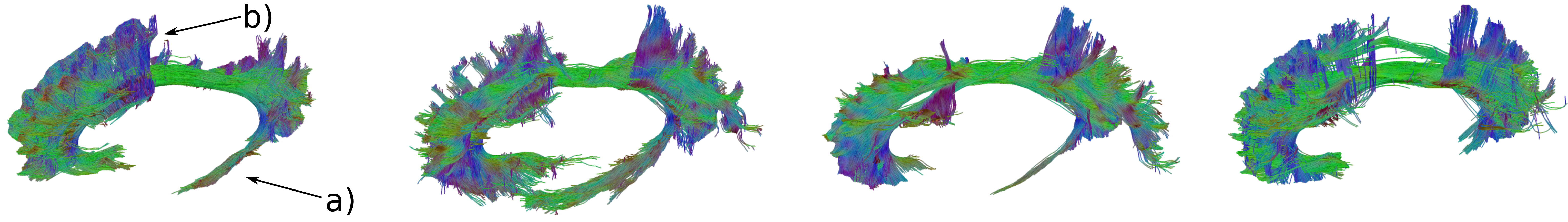
Figure 3: Reconstructions of the left Cingulum. From left to right: Reference, Bingham, Watson, low-rank UKF. The Bingham UKF permits the most complete reconstruction. The low-rank UKF misses the parahippocampal part a), while the Watson UKF misses fibers towards the anterior cingulate cortex b).

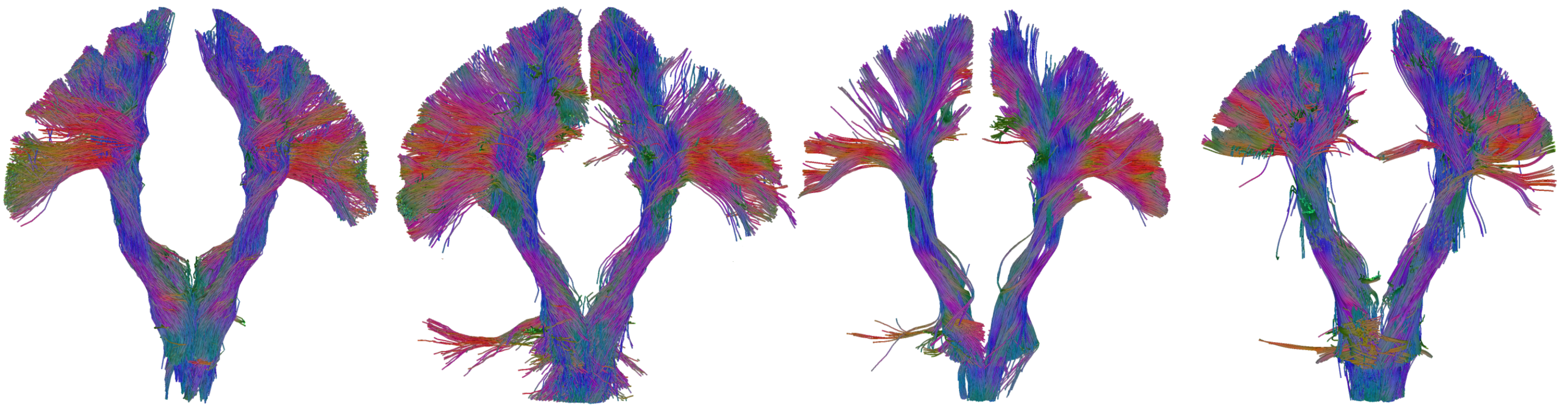
Figure 4: Reconstructions of the corticospinal tract (CST). From left to right: Reference, Bingham, Watson, low-rank UKF. The Bingham UKF leads to the highest streamline density in the lateral fanning.

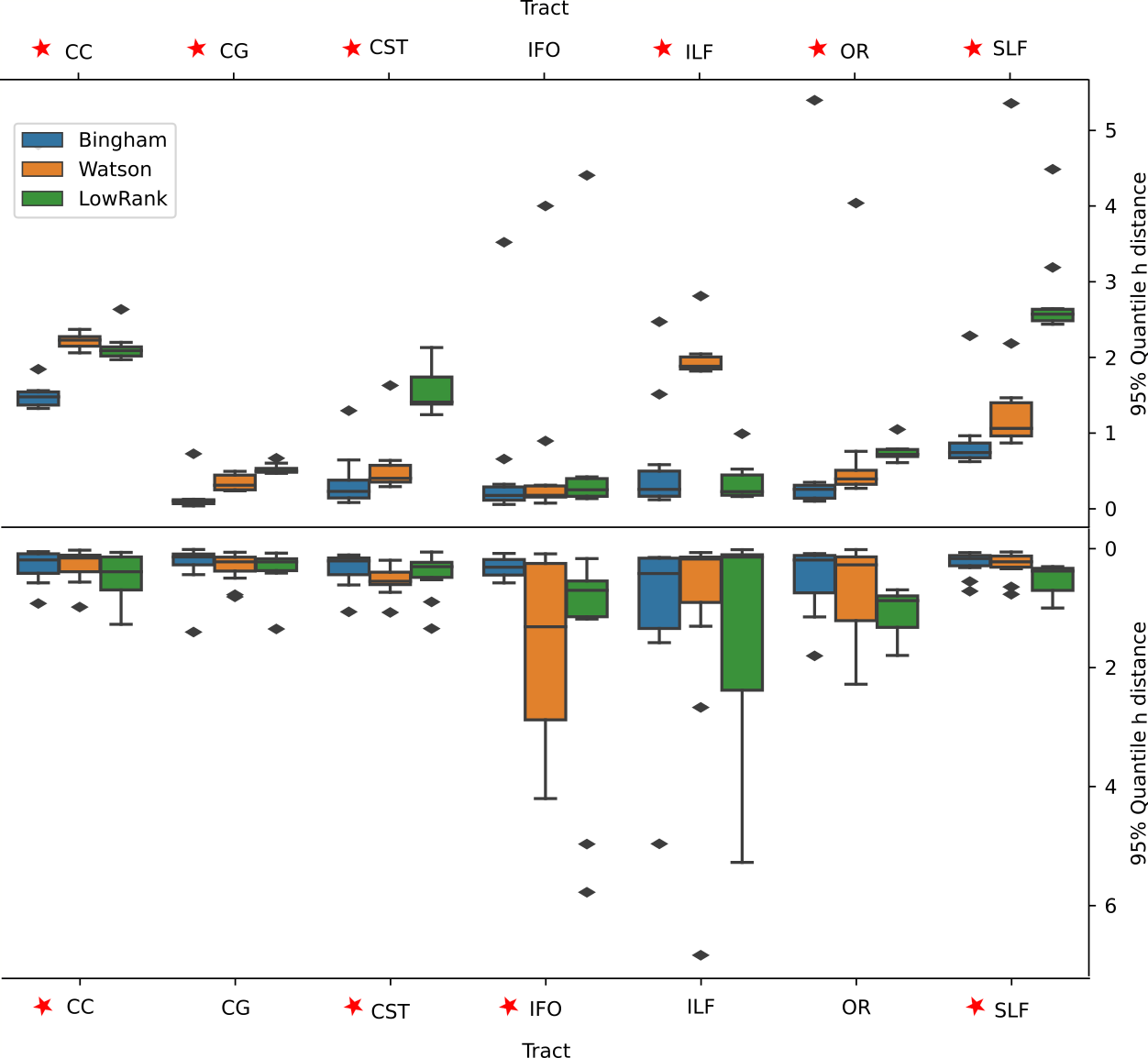
Figure 5: Top: 95% quantile of the directed Hausdorff distance from reference to reconstruction. Median distances are lowest, indicating highest completeness, for Bingham UKF in all tracts except the ILF. In 6 out of 7 tracts, differences are significant (asterisks). Bottom: Directed distance from reconstruction to reference. In most tracts, even these distances decrease when modeling fanning, indicating improved specificity in addition to the higher completeness.

We quantify these results by evaluating directed Hausdorff distances. The upper part of Figure 5 shows distances from the reference to the reconstruction. In 6 out of 7 tracts, the Bingham UKF exhibits the lowest median, indicating the most complete reconstructions. The lower part measures distances from the reconstruction to the reference, so that low values indicate low excess. In 6 out of 7 tracts, the Bingham UKF leads to a lower median than the low-rank UKF, indicating that specificity is improved in addition to the increased sensitivity.

To statistically assess the differences between the proposed methods, we conducted a Friedman test [8] for each tract. An asterisk denotes significant differences at significance level of $p<0.007$, due to Bonferroni correction. In 6 out of 7 tracts, we found significant differences in the completeness of reconstruction. In 4 out of 7 tracts, significant differences were observed for the excess.

Generation of 1000 CST streamlines took 92.5 seconds for the Bingham UKF, 85.2 seconds for the Watson UKF, and 58.1 seconds for the low-rank UKF on a single core of a 3.3 GHz CPU.

5 Conclusion

We developed a new algorithm for probabilistic tractography that incorporates anisotropic fanning into the recently described low-rank UKF. We demonstrated that this results in more complete reconstructions, while also reducing false positives, in almost all bundles. Our proposed technical solutions for initialization, convolution, and representation of rotations contribute to maintaining acceptable computational efficiency. Our code will be made available along with the publication.

References

- [1] Ankele, M., Lim, L.H., Groeschel, S., Schultz, T.: Versatile, robust, and efficient tractography with constrained higher-order tensor fODFs. Int’l J. of Computer Assisted Radiology and Surgery 12(8), 1257–1270 (2017). https://doi.org/10.1007/s11548-017-1593-6
- [2] Bernal-Polo, P., Martínez-Barberá, H.: Kalman filtering for attitude estimation with quaternions and concepts from manifold theory. Sensors 19(1), 149 (Jan 2019). https://doi.org/10.3390/s19010149
- [3] Bingham, C.: An antipodally symmetric distribution on the sphere. The Annals of Statistics 2(6), 1201–1225 (1974). https://doi.org/10.1214/aos/1176342874
- [4] Chen, Z., Tie, Y., Olubiyi, O.I., Zhang, F., Mehrtash, A., Rigolo, L., Kahali, P., Norton, I., Pasternak, O., Rathi, Y., Golby, A.J., O’Donnell, L.J.: Corticospinal tract modeling for neurosurgical planning by tracking through regions of peritumoral edema and crossing fibers using two-tensor unscented kalman filter tractography. Int’l J. of Computer Assisted Radiology and Surgergy 11(8), 1475–1486 (2016). https://doi.org/10.1007/s11548-015-1344-5
- [5] Cheng, G., Salehian, H., Forder, J.R., Vemuri, B.C.: Tractography from HARDI using an intrinsic unscented kalman filter. IEEE Trans. on Medical Imaging 34(1), 298–305 (2015). https://doi.org/10.1109/TMI.2014.2355138
- [6] Dalamagkas, K., Tsintou, M., Rathi, Y., O’Donnell, L., Pasternak, O., Gong, X., Zhu, A., Savadjiev, P., Papadimitriou, G., Kubicki, M., Yeterian, E., Makris, N.: Individual variations of the human corticospinal tract and its hand-related motor fibers using diffusion mri tractography. Brain Imaging and Behavior 14, 696–714 (2020). https://doi.org/10.1007/s11682-018-0006-y
- [7] Dell'Acqua, F., Tournier, J.D.: Modelling white matter with spherical deconvolution: How and why? NMR in Biomedicine 32(4) (2018). https://doi.org/10.1002/nbm.3945
- [8] Friedman, M.: The use of ranks to avoid the assumption of normality implicit in the analysis of variance. Journal of the American Statistical Association 32(200), 675–701 (1937). https://doi.org/10.1080/01621459.1937.10503522
- [9] Grün, J., Gröschel, S., Schultz, T.: Spatially Regularized Low-Rank Tensor Approximation for Accurate and Fast Tractography. NeuroImage 271 (2023). https://doi.org/10.1016/j.neuroimage.2023.120004
- [10] Huttenlocher, D., Klanderman, G., Rucklidge, W.: Comparing images using the hausdorff distance. IEEE Transactions on Pattern Analysis and Machine Intelligence 15(9), 850–863 (1993). https://doi.org/10.1109/34.232073
- [11] Jeurissen, B., Descoteaux, M., Mori, S., Leemans, A.: Diffusion MRI fiber tractography of the brain. NMR in Biomedicine 32(4), e3785 (2019). https://doi.org/10.1002/nbm.3785
- [12] Julier, S., Uhlmann, J.: Unscented filtering and nonlinear estimation. Proceedings of the IEEE 92(3), 401–422 (2004). https://doi.org/10.1109/JPROC.2003.823141
- [13] Kaden, E., Knösche, T.R., Anwander, A.: Parametric spherical deconvolution: Inferring anatomical connectivity using diffusion MR imaging. NeuroImage 37(2), 474–488 (2007). https://doi.org/10.1016/j.neuroimage.2007.05.012
- [14] Kraft, E.: A quaternion-based unscented kalman filter for orientation tracking. In: Sixth International Conference of Information Fusion, 2003. Proceedings of the. vol. 1, pp. 47–54 (2003). https://doi.org/10.1109/ICIF.2003.177425
- [15] Maier-Hein, K., Neher, P., Houde, J.C., Côté, M.A., Garyfallidis, E., Zhong, J., Chamberland, M., Yeh, F.C., Lin, Y.C., Ji, Q., Reddick, W., Glass, J., Chen, D., Yuanjing, F., Gao, C., Wu, Y., Ma, J., Renjie, H., Li, Q., Descoteaux, M.: The challenge of mapping the human connectome based on diffusion tractography. Nature Communications 8, 1349 (11 2017). https://doi.org/10.1038/s41467-017-01285-x
- [16] Malcolm, J., Shenton, M., Rathi, Y.: Filtered multitensor tractography. IEEE Transactions on Medical Imaging 29, 1664–75 (09 2010). https://doi.org/10.1109/TMI.2010.2048121
- [17] Malcolm, J.G., Michailovich, O., Bouix, S., Westin, C.F., Shenton, M.E., Rathi, Y.: A filtered approach to neural tractography using the watson directional function. Medical Image Analysis 14(1), 58–69 (2010). https://doi.org/10.1016/j.media.2009.10.003
- [18] Riffert, T.W., Schreiber, J., Anwander, A., Knösche, T.R.: Beyond fractional anisotropy: Extraction of bundle-specific structural metrics from crossing fiber models. NeuroImage 100, 176–191 (2014). https://doi.org/10.1016/j.neuroimage.2014.06.015
- [19] Schultz, T., Kindlmann, G.: A maximum enhancing higher-order tensor glyph. Computer Graphics Forum 29(3), 1143–1152 (2010). https://doi.org/10.1111/j.1467-8659.2009.01675.x
- [20] Schultz, T., Seidel, H.P.: Estimating crossing fibers: A tensor decomposition approach. IEEE Transactions on Visualization and Computer Graphics 14(6), 1635–1642 (2008). https://doi.org/10.1109/TVCG.2008.128
- [21] Sotiropoulos, S.N., Behrens, T.E., Jbabdi, S.: Ball and rackets: Inferring fiber fanning from diffusion-weighted MRI. NeuroImage 60(2), 1412–1425 (2012). https://doi.org/10.1016/j.neuroimage.2012.01.056
- [22] Tournier, J.D., Calamante, F., Connelly, A.: Robust determination of the fibre orientation distribution in diffusion MRI: Non-negativity constrained super-resolved spherical deconvolution. NeuroImage 35(4), 1459–1472 (2007). https://doi.org/10.1016/j.neuroimage.2007.02.016
- [23] Van Essen, D.C., Smith, S.M., Barch, D.M., Behrens, T.E., Yacoub, E., Ugurbil, K.: The WU-Minn human connectome project: An overview. NeuroImage 80, 62–79 (2013). https://doi.org/10.1016/j.neuroimage.2013.05.041
- [24] Wakana, S., Caprihan, A., Panzenboeck, M.M., Fallon, J.H., Perry, M., Gollub, R.L., Hua, K., Zhang, J., Jiang, H., Dubey, P., Blitz, A., van Zijl, P., Mori, S.: Reproducibility of quantitative tractography methods applied to cerebral white matter. NeuroImage 36, 630–644 (2007). https://doi.org/10.1016/j.neuroimage.2007.02.049
- [25] Wasserthal, J., Neher, P., Maier-Hein, K.H.: Tractseg - fast and accurate white matter tract segmentation. NeuroImage 183, 239–253 (2018). https://doi.org/10.1016/j.neuroimage.2018.07.070
- [26] Wiener, T.F.: Theoretical analysis of gimballess inertial reference equipment using delta-modulated instruments. Ph.D. thesis, Massachusetts Institute of Technology (1962)