Inference for Projection Parameters in Linear Regression:
beyond
Abstract
We consider the problem of inference for projection parameters in linear regression with increasing dimensions. This problem has been studied under a variety of assumptions in the literature. The classical asymptotic normality result for the least squares estimator of the projection parameter only holds when the dimension of the covariates is of a smaller order than , where is the sample size. Traditional sandwich estimator-based Wald intervals are asymptotically valid in this regime. In this work, we propose a bias correction for the least squares estimator and prove the asymptotic normality of the resulting debiased estimator. Precisely, we provide an explicit finite sample Berry Esseen bound on the Normal approximation to the law of the linear contrasts of the proposed estimator normalized by the sandwich standard error estimate. Our bound, under only finite moment conditions on covariates and errors, tends to 0 as long as up to the polylogarithmic factors. Furthermore, we leverage recent methods of statistical inference that do not require an estimator of the variance to perform asymptotically valid statistical inference and that leads to a sharper miscoverage control compared to Wald’s. We provide a discussion of how our techniques can be generalized to increase the allowable range of even further.
1 Introduction
Linear regression is a fundamental statistical tool that has been widely used in various fields of research. The classical literature on linear regression studies the ordinary least square (OLS) estimation has focused primarily on the well-specified case, where the underlying truth postulates the linear relation between the response variable and covariates. As elucidated in works in an assumption-lean framework (Berk et al., 2019; Vansteelandt and Dukes, 2022), although the model assumption sometimes takes account of the pre-knowledge, the usage of model assumptions is dishonest when used because of the mathematical convenience. As real data often possess a highly nonlinear structure, relying on model assumptions and considering them as representing ground truth in inference may be problematic. Compared to the popularity of parametric regression in both practical studies in statistics and econometrics, the theoretically established properties of regression coefficients in an assumption-lean framework have just started to gain attraction. To this effort, some approaches start with a traditional estimator of a parameter indexing a parametric regression model and then characterize what estimand the estimator converges to, without assuming that the model is true (Kuchibhotla et al., 2020; Berk et al., 2019). In particular, we focus on misspecified linear regression models comprised of a -dimensional random vector of covariates and a scalar random variable . If admits the second moment, then the conditional expectation , which is not necessarily linear, is the best approximation to among functions of . It is well known that the best linear approximation to is the linear function is well-defined where the coefficients is given by
Provided that the population Gram matrix is invertible, the solution is unique and given by the vector of projection parameters (Buja et al., 2019a, b),
where . The projection parameter is traditionally estimated using the ordinary least square estimator (OLSE). Suppose that we observe a sample of i.i.d observations from . Then, the OLSE is defined as
Provided that the sample Gram matrix is invertible with probability 1, then the OLSE is well-defined and can be expressed as
where .
1.1 Related Works
Asymptotic Normality and Berry Esseen bound for the Least Square Estimator
In fixed-dimensional settings, the OLSE has been the subject of large sample theory and conventional Berry-Esseen bounds, demonstrated by Van der Vaart (2000) and Pfanzagl (1973), respectively. With increasing dimensions, Bickel and Freedman (1983) established the asymptotic normality of the least squares and the consistency of bootstrap, requiring under a well-specified linear model with fixed covariates and homogeneous errors. Additionally, a series of papers by Portnoy (1984, 1985, 1986, 1988) showcased various consistency and asymptotic normality properties for estimators, including M-estimators and maximum likelihood estimators. Translating these findings into our context mandates to ensure the -consistency of the OLSE within a well-specified model under a set of arguably strong assumptions on the data-generating process. In a more general setting, albeit postulating at least a partially linear model, the asymptotic normality of (non-)studentized OLSE has been investigated with additional regularity conditions on covariates and errors (Donald and Newey, 1994; Cattaneo et al., 2015, 2018a, 2018b). This reference list is far from complete. Some of these works pertain to the regime and occasionally allow the boundary case of .
An initial step toward the misspecified linear model with minimal assumptions on covariates and errors was made in Mammen (1993). They were concerned with linear contrasts of the regression coefficients and asserted the consistency of both the resampling bootstrap and the wild bootstrap in estimating the regression coefficient with increasing dimensions. They claimed that is sufficient for consistent resampling bootstrap and that for the wild bootstrap. While their work provides useful intuition regarding the asymptotic behavior of the OLSE under model misspecification, their findings rely on heuristics and do not explicitly present the convergence rate. Rinaldo et al. (2019) formulated the Berry Esseen bound for general nonlinear statistics under the misspecified setting. Their analysis, specifically applied to projection parameters, established a uniform Berry Esseen bound for entry-wise asymptotic normality of the Ordinary Least Square Estimator (OLSE), converging to under , disregarding polylogarithmic factors (refer to Theorem 2 therein). More recently, Kuchibhotla et al. (2020) derived a novel finite sample bound for the studentized OLSE under finite moment assumptions on covariates and errors. They obtained a uniform Berry Esseen bound for entry-wise asymptotic normality of the OLSE, with their bound scaling as , disregarding polylogarithmic factors and under sufficient moment conditions on covariates and errors; See Theorem 10 of Kuchibhotla et al. (2020). Consequently, they required for the bound to vanish, facilitating the construction of simultaneous confidence intervals for the projection parameter coefficients under such dimension range. Notably, these intervals can exhibit a width of the order . It should be emphasized that the parameters of interest in this article are linear contrasts of the projection parameters which are different from those addressed in Rinaldo et al. (2019) and Kuchibhotla et al. (2020).
De-biasing of the Least Square Estimator
Under misspecified linear models, extensive attention has focused on scenarios where , with limited exploration beyond this scaling despite the OLSE remaining well-defined for . In cases where , the OLSE demonstrates a bias of order (Mammen, 1993; Cattaneo et al., 2019), impeding valid inference on regression parameters without de-biasing. To tackle this, Cattaneo et al. (2019) proposed the bias-corrected -estimator via the Jackknife method, ensuring consistency and asymptotic normality of the two-step point estimate under , presenting bootstrap-based inferential methods as well.
The term “de-biasing” typically refers to a correction applied to the original regularized estimator, often necessary to resist the curse of dimensionality or to enhance prior knowledge about the geometric/intrinsic structure of data. Common examples in linear regression include the LASSO, ridge, and SLOP estimators. It is worth emphasizing that “de-biasing” here aims to address the “bias” mainly induced by model misspecification at the population level rather than a specific regularization technique.
Variance Estimation
In the context of linear regression, the inflating variance of regression coefficient estimates along with increasing dimension has prompted efforts to propose robust covariance estimates capable of accommodating dimensionality and potential heteroscedasticity. The degree-of-freedom-corrected covariance estimator, introduced by MacKinnon and White (1985), has served as a foundation for subsequent modifications within well-specified linear models, known as HC-class variance estimators. For comprehensive reviews of these estimators, we refer our readers to Long and Ervin (2000) and MacKinnon (2012). Recent additions to the HC class include the HCK estimator proposed by Cattaneo et al. (2018b) and the HCA estimator proposed by Jochmans (2022). However, in both cases, consistency of variance estimate requires a dimensionality constraint of in misspecified linear models, albeit under different settings. Under a very similar setting to ours, Kuchibhotla et al. (2020) noted that a dimensionality requirement of appears to be unavoidable for the consistency of the sandwich estimator for the OLSE variance (see Lemma 8 of Kuchibhotla et al. (2020)).
1.2 Contributions
In this paper, we employ an assumption-lean framework to offer a finite-sample distribution approximation for the projection parameter, imposing minimal assumptions. Specifically, our focus centers on estimating and inferring a scalar parameter in a predetermined direction . The main contributions of this study are summarized as follows.
-
•
We propose a bias-corrected least square estimator for the projection parameter. Theorem 3 presents the Berry Esseen bound for the approximation to the adjusted Normal distribution of the unnormalized linear contrast of the proposed estimator, and the bound is sharp and roughly scales like
(1) provided that and , where and represent the finite moments of the covariate and the error , respectively; See also Corollary 1. Consequently, achieving the vanishing bound necessitates the scaling , strictly embracing the traditional requirement of . Our result, to the best of our knowledge, presents the sharpest bound under the (possibly) misspecified linear model while relying on the weakest assumptions regarding the true data distribution.
-
•
While the Berry Esseen bound presented in Theorem 3 involves the unknown parameter for the asymptotic variance of the proposed estimator, Section 4 outlines at least two inference methods for constructing (non-)asymptotically valid confidence intervals. These methods do not necessitate estimating the asymptotic variance, thereby enabling us to utilize the sharp Berry Esseen bound from Theorem 3. Our approach involves inferential techniques based on resampling and sample splitting, including HulC (Kuchibhotla et al., 2021), statistic based inference (Ibragimov and Müller, 2010; Lam, 2022), and wild bootstrap (Wu, 1986; Mammen, 1993). We also illustrate these proposed methods through empirical examples in Section 5.
-
•
Our main result, Theorem 5, establishes a finite-sample Berry-Esseen bound for a studentized linear contrast of the bias-corrected estimator under the assumptions of finite moments for both the covariates and the errors. Our bound, disregarding the polylogarithmic factors, roughly scales as follows:
(2) provided that and ; See also Corollary 2. Our bound immediately leads to the validity of the Wald confidence interval for a linear contrast of the projection parameters as outlined in Corollary 3.
The slower convergence rate outlined in (2) compared to that in (1) is solely due to the additional convergence rate introduced by the sandwich variance estimator. However, it is noteworthy that the consistency of the sandwich variance estimator does not demand any additional dimension scaling beyond . Moreover, as per Theorem 4, the sandwich variance estimator attains consistency if . To the best of our knowledge, our result on the consistency of the sandwich variance estimator allows the broadest range of dimension scaling in assumption lean linear regression literature.
-
•
One of the key quantities in our analysis is , representing the difference between the population and the sample gram matrix in the operator norm. We introduce a new concentration inequality for under finite moment assumptions on covariates (), detailed in Proposition 22. This result is inspired by recent findings on the universal spectral properties of random matrices, relating them to Gaussian random matrices with identical mean and covariance in their entries (Brailovskaya and van Handel, 2023). Our bound for matches the sharpness (up to polylogarithmic factors) of the one provided in Tikhomirov (2018), regarded as the sharpest to date. Notably, our bound avoids the necessity for a ‘large’ to ensure a ‘high’ probability concentration of the sample Gram matrix. Section B.3 outlines the historical context of and offers a comparison of concentration inequalities in this regard.
1.3 Organization
The remainder of this paper is organized as follows: Section 2.1 introduces the problem setup and notations, while Section 2.2 outlines the distributional assumptions on the data generating process. Our primary result on the Berry Esseen bound for the distribution approximation of the law of the studentized linear contrast of the proposed estimator is presented in Section 3. Section 4 details several inferential methods for the projection parameter based on the bootstrap and sample splitting. Numerical results are provided in Section 5. The Appendix includes all proofs, technical lemmas, and additional numerical results.
2 Problem setup and Assumptions
2.1 Projection parameters
Let be an independent sample of observations. The projection parameter is defined as
| (3) |
The minimizer in (3) solves the linear equation that
| (4) |
If the population gram matrix is invertible, the projection parameter is well-defined and can be uniquely expressed as where . In the case where the observations follow the linear model with , the projection parameter corresponds to the model parameter, i.e., . On the contrary, if the underlying truth exhibits a possibly non-linear structure, then the projection parameter gives the best linear approximation to with respect to the joint distribution of . For a detailed discussion on the projection parameter and its interpretation, see Buja et al. (2019a, b).
The projection parameter is estimated using the ordinary least square estimator (OLSE) which follows the traditional definition that
If the sample population matrix is invertible with probability 1, then the OLSE is well defined and can be written as where .
Additional Notations
For two real numbers and , let , and . Let be the identity matrix. We let be the -dimensional vector of ones and be of zeros. For any , we write . In addition with a positive definite matrix , we denote the scaled Euclidean norm as . We let be the operator norm of the matrices. The unit sphere in is . The :th canonical basis of is written as for all . Convergence in distribution is denoted by and convergence in probability by . We write the smallest eigenvalue and the largest eigenvalue of the square matrices as and , respectively. The cumulative distribution function of the standard Normal distribution is denoted as and its :th derivative as for . Finally, we adopt the conventional asymptotic notations. Given two non-negative sequences of reals and , we write if there exists a constant and such that for any , , and if as . We sometimes write for , and for . Furthermore, for a sequence of random variables and a non-zero sequence , we write if as , and if for any , there exists and such that for all .
2.2 Assumptions
Our main results are built upon the following assumptions, primarily emphasizing minimal assumptions on the data generating process. These include moment conditions on both the response and covariates, thereby encompassing a wide range of distributions, such as heavy-tailed distributions and discrete distributions.
Assumption 1.
There exists some and a constant satisfying that
for .
Assumption 1 imposes a moment condition solely on the error, allowing for heteroscedastic errors that may arbitrarily depend on the covariates and even accommodate heavy-tailed errors. This assumption is prevalent in recent literature on heteroskedastic linear regression (Mourtada et al., 2022; Kuchibhotla and Patra, 2022; Han and Wellner, 2019; Mendelson, 2016). Additionally, it is often assumed that the conditional variance of the error is uniformly bounded almost everywhere, described by
| (5) |
where . Here, and are essential infimum and essential supremum, respectively, with respect to the marginal distribution of . Given (5), our results in the following section remain valid even under the relaxed moment assumptions on the covariates.
Assumption 2.a.
There exists some and a constant satisfying that
for and .
Assumption 2.b.
There exists a constant such that
for all and .
Assumption 2.c.
There exists some and a constant satisfying that
for and . Furthermore, , , have independent entries.
Assumption 2.a implies equivalence for one-dimensional marginals of covariates. This is a significant weakening of sub-Gaussianity in Assumption 2.b. It is common to impose when studying the linear regression with increasing dimensions (Oliveira, 2016; Catoni, 2016; Mourtada et al., 2022; Mourtada, 2022; Vaškevičius and Zhivotovskiy, 2023) even though we sometimes require a higher moment condition to analyze a higher order expansion of the least square estimate.
Furthermore, Assumption 2.a implies the bounded-ness of :th moment of the -norm of the random vector . To illustrate, note that for all . By applying Jensen’s inequality, we have:
which holds deterministically as long as . Consequently, it leads to
where the last inequality follows from Assumption 2.a. This also emphasizes that the appropriate scaling of is proportional to as the dimension grows.
Assumption 2.c assumes that -normalized covariates have independent entries, in addition to the moment conditions. Under Assumption 2.c, we can achieve a more precise control over the -norm of covariates (Rio, 2017) and the sample Gram matrix (Srivastava and Vershynin, 2013; Mendelson and Paouris, 2014).
Assumption 3.
Let
There exist constants satisfying that
Assumption 3 ensures that both and scale in a similar order, serving as the only technical assumption in our paper. This condition appears inevitable to prevent the asymptotic variance of the least square estimator from inflating or vanishing. Specifically, noting that the condition (5) is sufficient for Assumption 3 to be held.
3 Methods and Results
3.1 Approximation of the Sample Gram Matrix and Bias Characterization
In this section, we present an approximation of the distribution of for any . To be presented results are mostly invariant to the scaling of . However, we sometimes consider those with , which gives a proper normalization, for some .
Our analysis starts with the least square estimate , particularly by approximating the sample Gram matrix using Taylor series expansion. We note
(See Lemma 33 of Kuchibhotla et al. (2020).) Consequently, we get the following approximation of :
| (7) | |||||
The term (7) is the first-order approximation and is the average of influence function—with respect to the square loss—evaluated at independent data points. Using the conventional large sample approximation for the case when , the variability of can be well-represented only through the term (7), and the second order term (7) or higher order terms are negligible. In particular, (7) is responsible for the asymptotic normality of when . Here, however, the term (7) may create a non-vanishing bias when . To see this, we note that
| (8) | |||||
| (11) | |||||
The quantities in (11) and (11) are resulted from multiplying the individual terms in (8) with the same indices, while the quantity (11) corresponds to the cross-index product. It is noteworthy that (11) can be absorbed into the average of influence functions in (7) as it has an additional scaling factor . The quantity (11) is a mean-zero degenerate -statistic of order up to a scaling factor that converges to 1 as . Therefore, the only quantity that may have a non-zero mean is (11) and we denote this by
| (12) |
Under the control of and using Assumption 2.a and 1, respectively, the quantity scales like due the factor. Consequently, yields a non-degenerate bias when . By manually removing the bias, a linear contrast can be approximated by the sum of the average of influence functions and the degenerate second-order -statistics as
where
| (13) |
It is well known that -statistics of order are asymptotically normally distributed, and there has been a vast literature related to Normal approximations and the rates of convergence for -order -statistics. We refer the readers to Bentkus et al. (2009). In order to state our first theorem, we define
| (14) | |||||
| (15) |
for any . It should be emphasized that the parameter is invariant to the scaling of . That is, for . In addition, recall that is the cumulative distribution function of the standard Normal distribution and is the third order derivative of .
Theorem 1 states a Berry-Essen bound for the Normal approximation of a linear contrast with known bias .
Theorem 1.
Suppose that Assumption 1 holds for and that Assumption 3 holds.
-
(i)
Suppose further that Assumption 2.a holds for and , and assume . Then, there exists a constant such that
-
(ii)
Suppose further that Assumption 2.b holds. Then, there exists a constant such that
-
(iii)
Suppose further that Assumption 2.c holds for and , and assume . Then, there exists a constant such that
Furthermore, if , then there exists a constant such that
Remark 1.
The conventional Berry Esseen type inequality implies the proximity between the distribution of the law of the estimator and the Normal distribution. In contrast, we show a distribution approximation to the “adjusted” Normal distribution, allowing a more precise representation of the approximation. The degree of adjustment is determined by the parameter , which turns out to scale as (see Lemma 16). Hence, we can enhance the Berry-Esseen bound for the Normal approximation by incorporating an additional term of to the existing bounds in Theorem 1, but yielding a slower convergence rate. More importantly, under the well-specified linear model, i.e., , then it follows that from its definition in (15). Consequently, in this case, the presented Berry-Esseen bound in Theorem 1 can be employed for the Normal approximation as well.
Remark 2.
The last part of Theorem 1 says that the OLSE does not necessarily require de-biasing under Assumption 2.c with a sufficiently large finite moment of covariates and errors. To provide an intuition for this, let us consider the bias term in (12), which scales with its expected value . By examining the definition of the projection parameter, we can express as the covariance between two random variables:
An application of Cauchy Schwarz’s inequality yields that
| (16) |
The leading variance term on the right-hand side of (16), under the finite moment assumptions of covariates and errors, is . Meanwhile, the quantity generally scales as , resulting in . However, when an additional assumption of independent entries of covariates, i.e., Assumption 2.c, is satisfied, roughly follows distribution, thereby leading to . This significantly reduces the magnitude of the right-hand side of (16) to . Consequently, the expected bias (when scaled by ) is negligible if .
Remark 3.
Regarding the results under Assumptions 2.a and 2.c, we conjecture that the dependence on logarithmic factors of our bound is suboptimal. The presence of seemingly spurious logarithmic factors mainly stems from the concentration inequality we employ for the sample Gram matrix, described in Proposition 22 in Section B.3. Although Theorem 1.1 of Tikhomirov (2018) partially addresses our query when , its application to our context (see Proposition 23) requires further supposition: as .
Theorem 1 gives the Berry Essen bound for the linear contrast of the properly-debiased projection parameters under three different distributional assumptions on covariates. The first part of Theorem 1 regards the most general case which relies only on finite-moment assumptions. Ignoring the polylogarithmic factors, the Berry-Esseen bound tends to zero as long as
If , this reduces to and meets the dimension requirement for the vanishing Berry Esseen bound under Assumption 2.b of sub-Gaussianity. Moreover, under Assumption 2.c, the bound tends to 0 as for all , disregarding the polylogarithmic factors.
3.2 Bias Estimation
The result given in Theorem 1 is mostly of theoretical importance as the inequality yet involves unknown parameters through bias and asymptotic variance . Therefore, to do inference on , for e.g. building confidence region, it is necessary to incorporate the estimates of bias and variance in the Berry Esseen bound given in Theorem 1. To this effect, we consider a method of moment estimator for defined as
| (17) |
The next result provides the consistency rate for the bias estimate in high dimensions and under mild moment conditions. As elucidated in Remark 2, the OLSE does not necessitate a debiasing procedure under Assumption 2.c with a sufficient number of moments of covariates and errors. Therefore, the following results will consider the cases under Assumption 2.a and 2.b only.
Theorem 2.
Theorem 2 provides the finite sample concentration inequalities for the bias estimate. Inspecting the result under Assumption 2.a, with the choice of
which was intended to minimize the tail probability, the bias estimate is consistent if , ignoring the polylogarithmic factors. If , then the dimension requirement reduces to . If Assumption 2.a is replaced with Assumption 2.b, then the dimension requirement for the consistency becomes again ignoring the polylogarithmic factors.
3.3 Berry Esseen Bound for the Unnormalized Bias-corrected Estimator
Combining the error bound for the bias estimate from Theorem 2 with the Berry-Esseen bound in Theorem 1, we get to the next result, a uniform Berry-Esseen bound for the unnormalized bias-corrected OLS estimator. We denote the bias-corrected estimator for the projection parameters as
Theorem 3.
Theorem 3 presents the Berry Esseen bound for approximating the law of the unnormalized linear contrast of the bias-corrected LSE — with respect to any query vector — to the adjusted Normal distribution. To the best of our knowledge, our bound stands as the sharpest among Berry Esseen bounds applicable to existing estimators in the assumption-lean linear regression framework. Moreover, it accommodates the widest range of dimensions for vanishing bound.
Under the moment condition of Assumption 2.a, our bound converges to zero if , disregarding the polylogarithmic factors. This reduces to when . Furthermore, if the covariates are sub-Gaussian, the Berry Esseen bound tends to zero if , again ignoring the polylogarithmic factors. Comparing the Berry Essen bound of the bias-corrected estimator to the bound given in Theorem 1 when the bias is known, we observe that using the bias estimate does not impose a stricter dimension requirement. This is due to the fact that the dimension requirement for the -consistency of the bias estimate in Theorem 2 is less strict than that given in Theorem 1, as shown by the inequality: for . If , then the quantities on both sides coincide with 2/3, and thus, the bound converges to zero if .
The following corollary presents a simpler Berry Essen bound for the bias-corrected OLS estimator. We use as a shorthand for the inequality , where involves only the constants defined in the assumptions and log-polynomial factors of and .
Corollary 1.
Suppose that the assumptions made in Theorem 3(i) hold. Furthermore, if and , then
| (18) |
In addition, the approximation to the Normal distribution follows:
| (19) |
A slower rate in (19) for the Normal approximation in comparison to that in (18) stems from the incorporation of the adjustment term , which approximately scales at (See Lemma 16), into the bound. As discussed previously in Remark 1, however, if the linear model is correctly specified so that , then the bound provided in (18) can also be utilized for the Normal approximation.
The Berry Esseen bound in Theorem 3, despite its reliance on the unknown distribution parameter , does not hinder our ability to conduct inference on the projection parameter . We leverage recent statistical methodologies based on re-sampling or sample splitting to enable this inference, which remains unaffected by the uncertainty of . In Section 4, a series of distinct methods are introduced, illustrating and exemplifying this approach.
3.4 Consistency of the Sandwich Variance Estimator
Berry Esseen bound for the studentized bias-corrected LSE remains pertinent, notably in the construction of Wald-type confidence intervals. As previously discussed, accomplishing this entails devising an estimator for the asymptotic variance that ideally maintains consistency across a wide range of dimensions argued in Theorem 3. For a specified query vector , the asymptotic variance of can be approximated through , as asserted in Theorem 3. Notably, the matrix is commonly referred to as the ‘sandwich variance’ for OLS in a misspecified linear regression setting (White, 1980; Buja et al., 2019a). A natural estimator for the sandwich variance is its plug-in counterpart , termed the ‘sandwich variance estimator’, where is the sample Gram matrix and is expressed as:
To this end, we define for .
The consistency of the sandwich variance estimator has been studied under various model- and distributional- assumptions and has often been a stand-alone line of research. A recent significant finding in a closely related context is detailed in Lemma 7 of Kuchibhotla et al. (2020). In particular, they prove that under conditions where , up to polylogarithmic factors, provided that . Hence, directly applying their results to our scenario may be challenging, as we are considering situations beyond . Nevertheless, we have found that along a specific query vector , the estimator maintains consistency across a broader range of dimensions, as elucidated in the following theorem.
Theorem 4.
Remark 4.
The proof of Theorem 4 is extensive due to the complex nature of the sandwich variance estimator, encompassed in Section A.7. Theorem 4 primarily focuses on the concentration inequality for , with the pivotal deterministic inequality established in Lemma 7. This lemma argues that the difference between the plug-in sandwich variance estimate and its population counterparts can be deterministically bounded using several factors, including , , and , among others mentioned. Consequently, the proof relies on the concentration inequality of these quantities, which in themselves hold potential as areas of independent interest. The rate presented in Theorem 4 is a result of leveraging these concentration inequalities, aiming to achieve the widest possible scaling of in terms of . However, alternative choices remain viable.
Theorem 4 shows that for a given , the variance estimate is consistent for the asymptotic variance as long as
| (20) |
ignoring the polylogarithmic factors. Under the assumptions that and , it reduces to . This strictly embraces the one obtained in Theorem 3, but it should be emphasized that Theorem 3 relies on the moment conditions and .
3.5 Berry Esseen Bound for the Studentized Bias-corrected Estimator
The error bounds established for the sandwich variance estimator in Theorem 4 and the Berry Esseen bound derived in Theorem 3 help to derive the Berry Esseen bound for the studentized debiased LSE, leading to our main result Theorem 5. For easier comprehension, we present a simpler bound in Corollary 2.
Theorem 5.
Corollary 2.
Suppose that the assumptions made in Theorem 5 hold. Furthermore, if , , and , then
| (21) |
Here, is a shorthand for the inequality up to constants and log-polynomial factors of and .
Remark 5.
The bound provided in (21) consists of three terms, none of which entirely dominates the others. Specifically, when the dimension is relatively ‘small’, that is, if , the dominant factor in the bound becomes . In a moderately dimensional scenario, i.e., when , becomes the leading factor. However, in a ‘large’ dimension scenario where , the prevailing factor in the bound is .
One of the immediate consequences of Theorem 5 is the asymptotic validity of the Wald confidence interval for the linear contrast of the projection parameters. Define a level- Wald confidence interval with respect to a predetermined as
Corollary 3.
Suppose that assumptions made in Theorem 6 hold, and let and be as described therein. Then, the false coverage rate of Wald CI can be controlled as
for some . If , , and , then
4 Confidence Region for the Projection Parameter
In the previous section, we have shown that the bias-corrected least square estimator is asymptotically Normal distributed. In this section, we present three methods that do not require a consistent estimate of the asymptotic variance but still enable us to get valid confidence intervals for the linear contrasts of the projection parameters.
4.1 HulC
The HulC (Kuchibhotla et al., 2021) is a statistical method that computes confidence regions for parameters by constructing convex hulls around a set of estimates. Suppose that we split a sample of i.i.d observations into batches where each batch contains at least observations***Kuchibhotla et al. (2021) noted that the batches need not be equal-sized, but having approximately equal sizes yields good width properties.. Denote the bias-corrected least square estimators obtained from :th batch as for . For any , define the maximum median bias (Kuchibhotla et al., 2021) for as
A key idea of the HulC is that the event
occurs unless either of the following happens: (1) for all or (2) for all . Consequently, we get
Since the bias-corrected OLS estimator is asymptotically Normal as shown in Corollory 1, converges to the asymptotic median, which is . The detailed procedure for constructing confidence interval at level is described in Algorithm 1.
Theorem 6.
Suppose that the assumptions made in Theorem 3(i) hold, and denote the Berry Esseen bound given in Theorem 3(i) as . For any and with , let and assume . Let be the confidence interval returned by Algorithm 1. Then, the false coverage rate of HulC CI can be controlled as
for some constant . If and , then
Remark 6 (Comparison with Wald Confidence Interval).
The Wald CI and HulC CI are both (asymptotically) valid as demonstrated in Corollary 3 and Theorem 6, respectively. A notable distinction between them lies in the fact that the HulC CI does not require an estimate for the asymptotic variance. Furthermore, the HulC CI shows a sharper miscoverage rate due to its reliance on the ‘squared’ Berry Esseen bound in Theorem 3. Despite this, the HulC CI tends to be wider due to its robust nature, which can be empirically demonstrated in Section 5. Importantly, the expected width ratio of the HulC CI to the Wald CI approximately equals (Kuchibhotla et al., 2021), slowly diverging as , and reaching 1.55 for the conventional choice of . A more comprehensive comparison can be found in Section 2.3 of Kuchibhotla et al. (2021).
Require: data , target coverage , and a query vector .
Ensure: A confidence interval for
4.2 -statistic based Inference
As in the previous section, consider partitions of observations. Here, the number of batches does not necessarily depend on the target coverage , and suppose that each batch has at least observations. Denote by the bias-corrected estimator of using observations in batch , . Since estimators are obtained independently, this amounts to the convergence of the joint distribution;
as if the dimension requirement in Theorem 3 are met. Hence, we can form an asymptotically valid confidence region based on the -statistic,
where and . By the continuous mapping theorem (Billingsley, 2013, Theorem 2.7), the given statistic is asymptotically -distributed with -degrees of freedom. By implication, the confidence interval for is given by
where denotes the upper th quantile of -distribution with degrees of freedom.
4.3 Bootstrap Inference
This section presents a method for carrying out post-bias-correction inference in our scenario, based on a bootstrap approach. Specifically, we utilize the wild bootstrap technique (Wu, 1986) to derive a computationally efficient approximation of the distribution of the bias-corrected OLS estimator. The idea is, as the residual bootstrap, to leave the covariates at their sample value, but to resample the response variable based on the residual values. First, we compute from the original dataset that the OLS estimator and the residuals for . For , let be i.i.d. bootstrap weights such that , , and . Then, we generate a bootstrap sample of observations by letting
for . Although Bootstrap weights are often drawn from the standard Normal distribution, we made use of the asymmetric weights in Section 5, which was proposed in Mammen (1993); and . Let estimator be the bias-corrected least square estimator based on bootstrap observations,
where and are bootstrap counterparts of the OLS estimator and estimated bias, respectively;
To construct the confidence interval, let where is the bootstrap bias-corrected estimator in :th simulation. The wild bootstrap level bias-corrected confidence interval for is given by
where is the empirical upper :th quantile of with .
Remark 7.
The validity of the above wild bootstrap inference may require additional dimension requirements. Theorem 1 of Mammen (1993) shows that wild bootstrap provides a consistent estimation of the unconditional distribution of in a well-specified linear regression model, without any bias correction, under the condition that . More recently, Theorem 11 of Kuchibhotla et al. (2020) establishes a finite sample approximation of the conditional bootstrap distribution of the law of OLSE in a similar setting to ours. In particular, the proof utilizes the Gaussian comparison bound (Lopes, 2020) to compare the conditional distribution of the bootstrap estimate with the Normal distribution. However, the estimation of asymptotic variance appears to be inevitable in the process, and this adds an additional dimension requirement of , particularly when and (see Lemma 10 of Kuchibhotla et al. (2020)). Furthermore, although not discussed in a linear regression context, Lemma 4.1 of Zhilova (2020) gives a sequence of random variables that justifies the necessity of the condition for the consistency of the wild bootstrap when estimating sample mean.
5 Numerical Studies
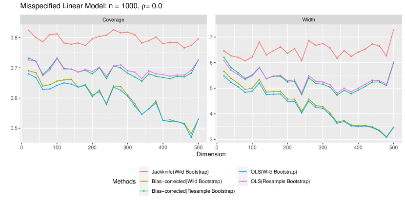
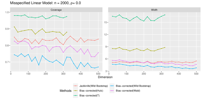
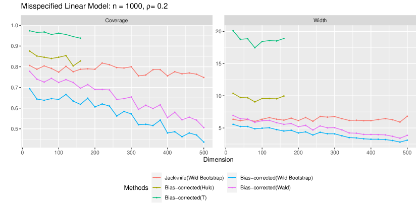
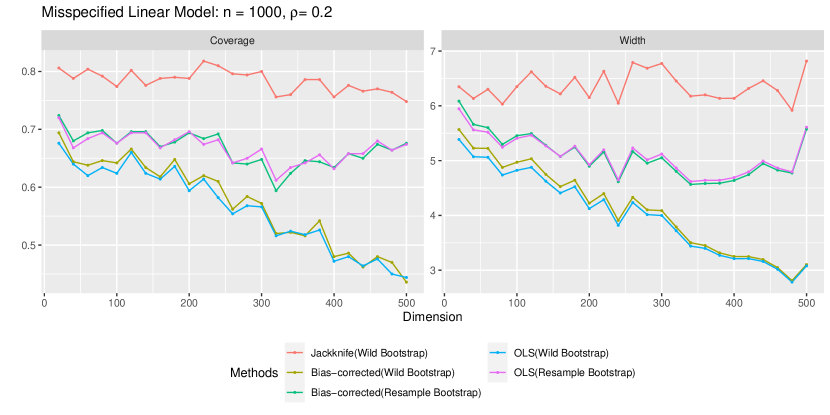
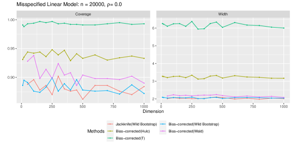
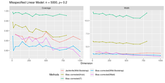
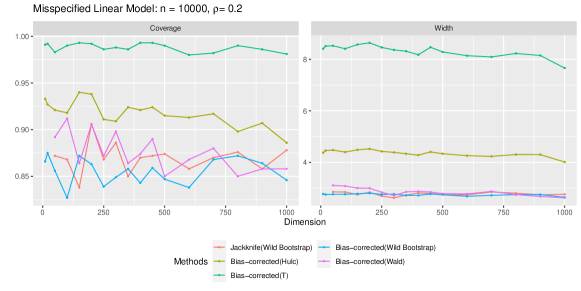
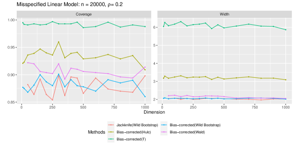
In this section, we compare the empirical coverages and widths of the 95% confidence intervals obtained from three inferential methods discussed in Section 4. Furthermore, we also compare the bootstrap confidence interval based on the jackknife-debiased OLS proposed in Cattaneo et al. (2019). In our specific simulation settings, which will be described shortly, we discovered that when leveraged with the bootstrap inferential methods, the jackknife-based debiased OLSE slightly outperforms the OLSE and the proposed bias-corrected OLSE. A large set of implementations, including both resampling bootstrap- and wild bootstrap-based confidence intervals using the OLS and the proposed debiased OLS, are presented in Appendix D.
5.1 Well-specified Linear Model
This section concerns the well-specified linear model. The simulation setting is as follows: for and , independent observations , , are generated as
where is the first coordinate of , that is, . Thus, the response relies only on the first dimension of and independent error . As the given model is well-specified, the projection parameter is given by .
Figure 1 compares the empirical coverage and the width of the 95% confidence intervals of the first coordinate of , which is 2, obtained from various methods. It is noteworthy that our bias-corrected estimator when incorporated with HULC achieves the target coverage of 0.95. On the contrary, the -statistic-based confidence interval seems to be fairly conservative while the wild bootstrap inference yields a seemingly less conservative confidence interval.

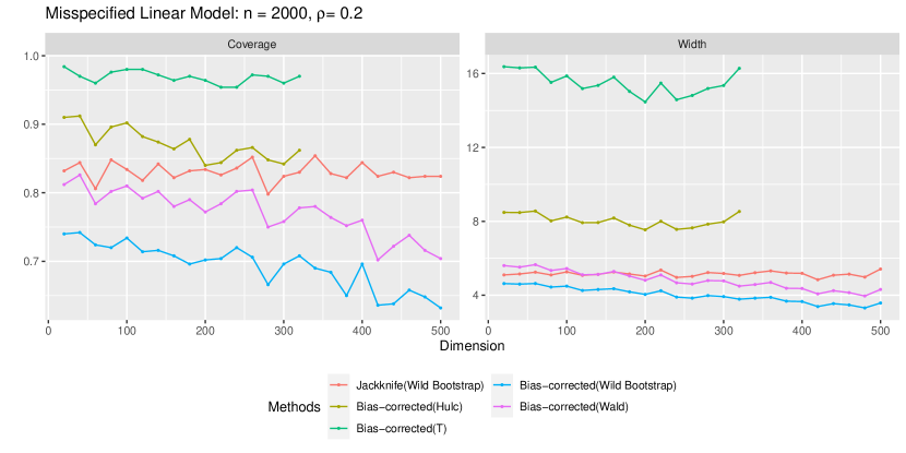
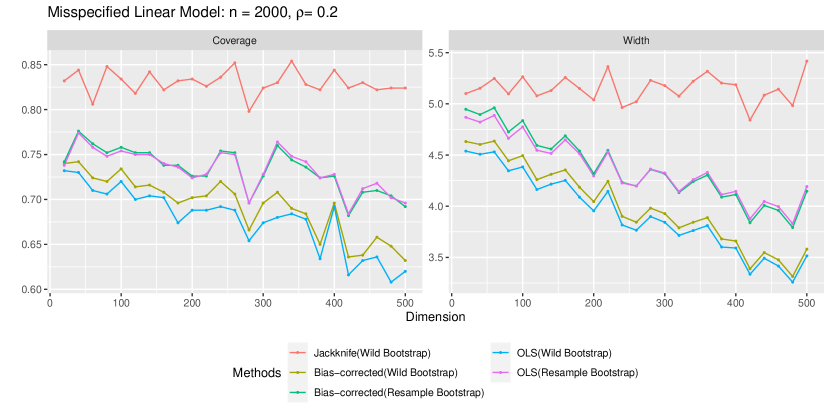
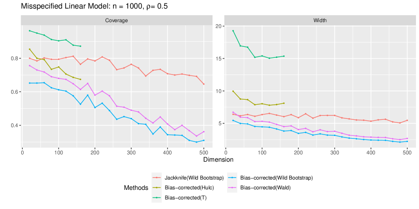
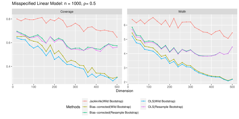
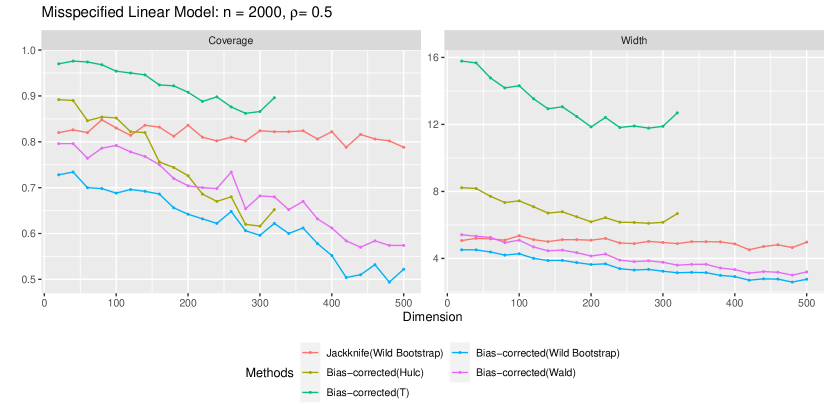
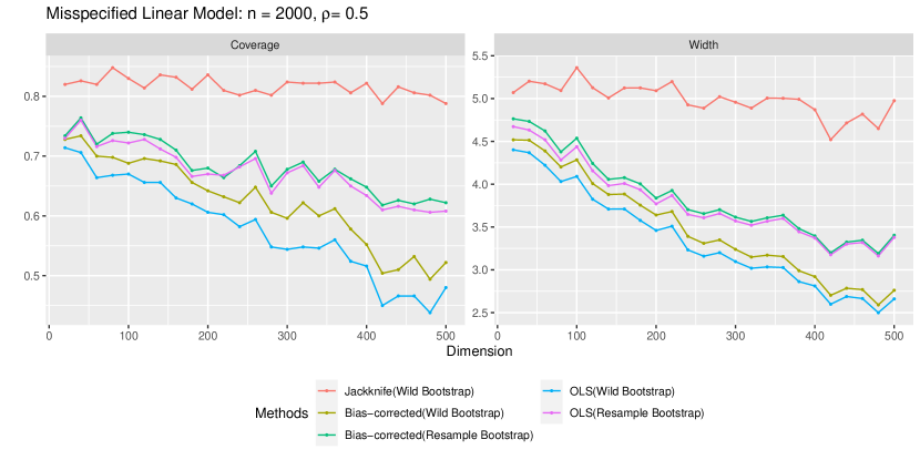
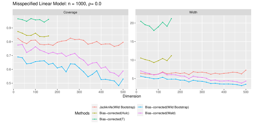
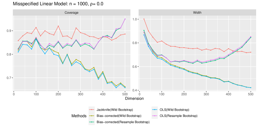
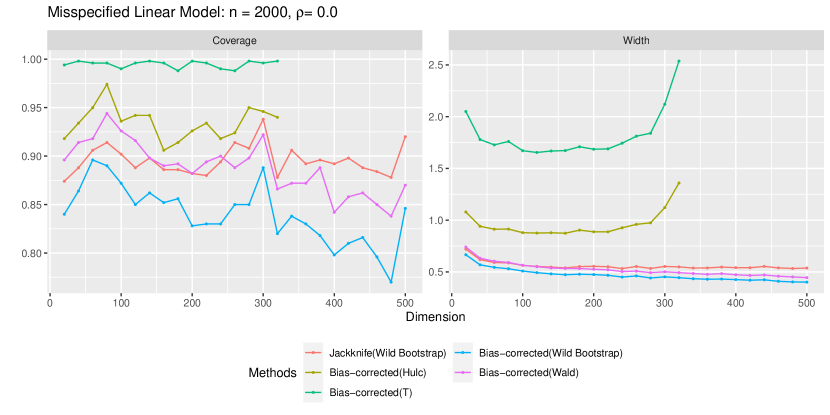
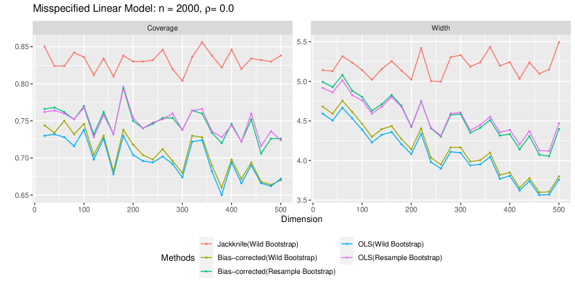
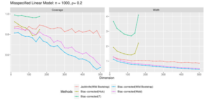
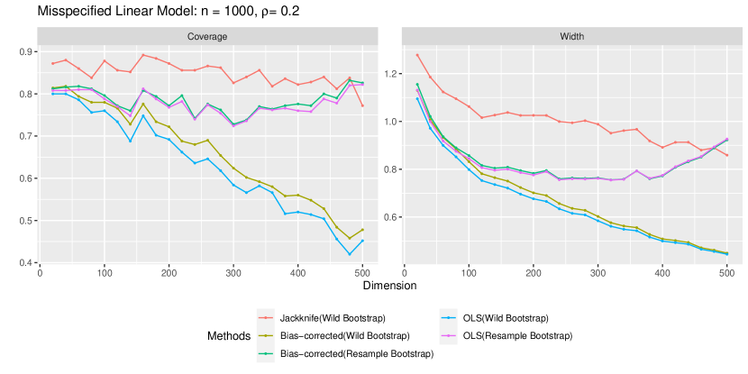
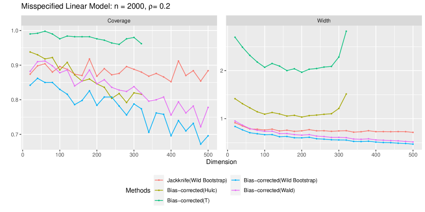
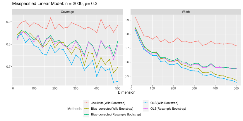
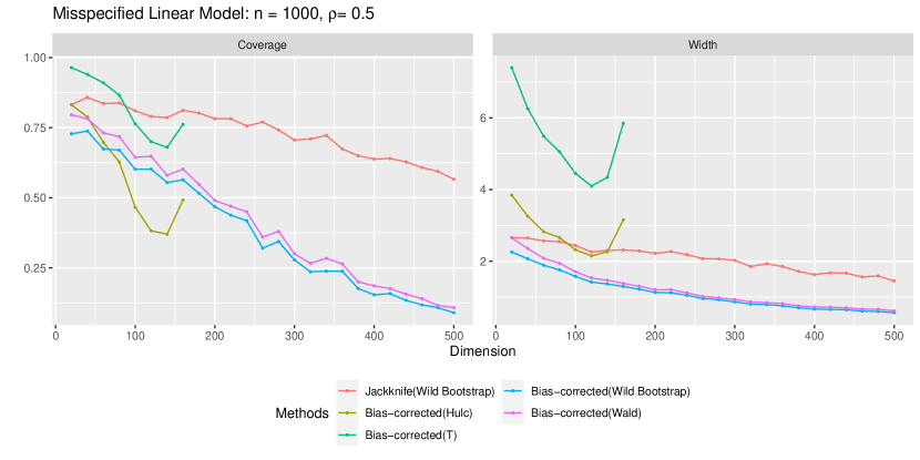
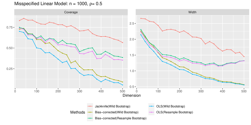
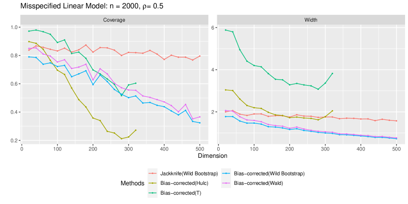
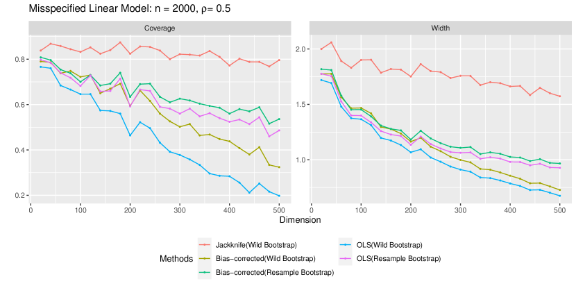
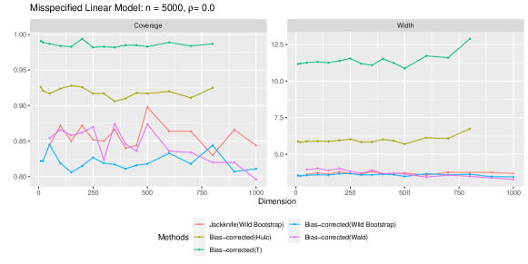
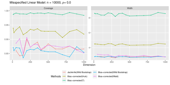
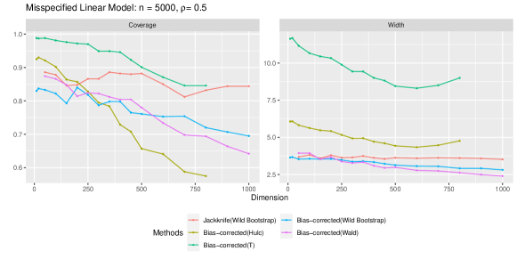
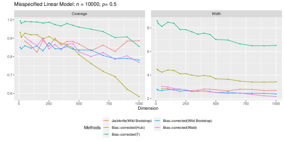
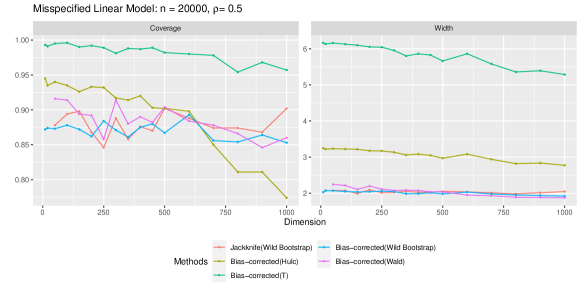
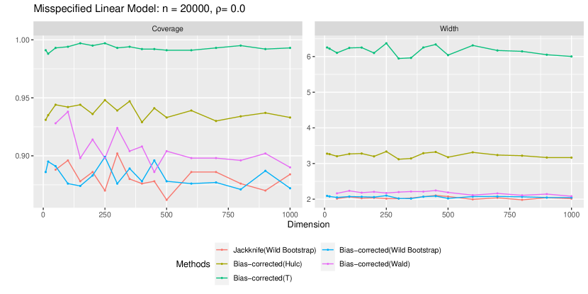
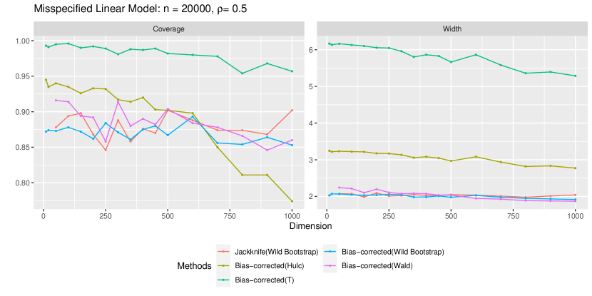
5.2 Misspecified Model
In this section, we concern about a misspecified non-linear model. The data-generating process for individual observation is as follows. We first independently generate two -dimensional Gaussian random vector
Here, the covariance matrix of , , is a compound symmetry where the diagonal entries are all and the off-diagonal elements are all for . That is, . We define the covariate vector as where denotes the entry-wise product. Then, the entries of are uncorrelated, i.e., , but not necessarily independent except the case when . For a -dimensional parameter , we let
| (22) |
where and is independent with and .
Under the aforementioned data-generating process, we conducted comprehensive experiments with the following sample sizes, dimensions, , and ;
Under the model (22), the projection parameter has the closed-form representation and turns out to be determined by and as,
where (see Lemma 28). The linear contrast of interest was set to which becomes the first coordinate of when and becomes the scaled average of coefficients of when . Furthermore, we can show that
Figure 2 compares the coverage and length of the 95% confidence intervals for under the setting where , , and or . Results under different combinations of sample size, dimension, , and are contained in Appendix D.
6 Discussion
We provide an estimator for the bias of the ordinary least squares estimator that is consistent as long as the dimension grows slower than , where is the sample size. The resulting debiased least squares estimator, after proper normalization, is asymptotically Normal at an -rate as long as . We also provide valid inference along any arbitrary direction for the projection parameter without having to estimate the variance. We achieve this inferential goal by leveraging the methods such as HulC. We believe the results of this paper can be extended to further expand the allowed growth rate of dimension. This extension would involve further expansion of the least squares estimator into higher order -statistics and removing the bias.
Acknowledgements.
A. K. Kuchibhotla and A. Rinaldo were partially supported by NSF DMS-2113611.
References
- Abdalla (2023) Pedro Abdalla. Covariance estimation under missing observations and moment equivalence. arXiv preprint arXiv:2305.12981, 2023.
- Adamczak et al. (2010) Radosław Adamczak, Alexander Litvak, Alain Pajor, and Nicole Tomczak-Jaegermann. Quantitative estimates of the convergence of the empirical covariance matrix in log-concave ensembles. Journal of the American Mathematical Society, 23(2):535–561, 2010.
- Bentkus et al. (2009) Vidmantas Bentkus, Bing-Yi Jing, and Wang Zhou. On normal approximations to U-statistics. The Annals of Probability, 37(6):2174 – 2199, 2009.
- Berk et al. (2019) Richard Berk, Andreas Buja, Lawrence Brown, Edward George, Arun Kumar Kuchibhotla, Weijie Su, and Linda Zhao. Assumption lean regression. The American Statistician, 2019.
- Bickel and Freedman (1983) Peter J Bickel and David A Freedman. Bootstrapping regression models with many parameters. Festschrift for Erich L. Lehmann, pages 28–48, 1983.
- Billingsley (2013) Patrick Billingsley. Convergence of probability measures. John Wiley & Sons, 2013.
- Brailovskaya and van Handel (2023) Tatiana Brailovskaya and Ramon van Handel. Universality and sharp matrix concentration inequalities, 2023.
- Buja et al. (2019a) Andreas Buja, Lawrence Brown, Richard Berk, Edward George, Emil Pitkin, Mikhail Traskin, Kai Zhang, and Linda Zhao. Models as approximations I: Consequences illustrated with linear regression. Statistical Science, 34(4):523–544, 2019a.
- Buja et al. (2019b) Andreas Buja, Lawrence Brown, Arun Kumar Kuchibhotla, Richard Berk, Edward George, and Linda Zhao. Models as approximations II: A model-free theory of parametric regression. Statistical Science, 34(4):545–565, 2019b.
- Catoni (2016) Olivier Catoni. Pac-bayesian bounds for the gram matrix and least squares regression with a random design. arXiv preprint arXiv:1603.05229, 2016.
- Cattaneo et al. (2015) Matias D Cattaneo, Michael Jansson, and Whitney K Newey. Treatment effects with many covariates and heteroskedasticity. Technical report, cemmap working paper, 2015.
- Cattaneo et al. (2018a) Matias D Cattaneo, Michael Jansson, and Whitney K Newey. Alternative asymptotics and the partially linear model with many regressors. Econometric Theory, 34(2):277–301, 2018a.
- Cattaneo et al. (2018b) Matias D Cattaneo, Michael Jansson, and Whitney K Newey. Inference in linear regression models with many covariates and heteroscedasticity. Journal of the American Statistical Association, 113(523):1350–1361, 2018b.
- Cattaneo et al. (2019) Matias D Cattaneo, Michael Jansson, and Xinwei Ma. Two-step estimation and inference with possibly many included covariates. The Review of Economic Studies, 86(3):1095–1122, 2019.
- Donald and Newey (1994) S.G. Donald and W.K. Newey. Series estimation of semilinear models. Journal of Multivariate Analysis, 50(1):30–40, 1994. ISSN 0047-259X. doi: https://doi.org/10.1006/jmva.1994.1032. URL https://www.sciencedirect.com/science/article/pii/S0047259X84710323.
- Einmahl and Li (2008) Uwe Einmahl and Deli Li. Characterization of LIL behavior in Banach space. Transactions of the American Mathematical Society, 360(12):6677–6693, 2008.
- Guédon and Rudelson (2007) Olivier Guédon and Mark Rudelson. Lp-moments of random vectors via majorizing measures. Advances in Mathematics, 208(2):798–823, 2007.
- Guédon et al. (2017) Olivier Guédon, Alexander E Litvak, Alain Pajor, and Nicole Tomczak-Jaegermann. On the interval of fluctuation of the singular values of random matrices. Journal of the European Mathematical Society (EMS Publishing), 19(5), 2017.
- Han and Wellner (2019) Qiyang Han and Jon A Wellner. Convergence rates of least squares regression estimators with heavy-tailed errors. The Annals of Statistics, 47(4):2286–2319, 2019.
- Ibragimov and Müller (2010) Rustam Ibragimov and Ulrich K Müller. t-statistic based correlation and heterogeneity robust inference. Journal of Business & Economic Statistics, 28(4):453–468, 2010.
- Jochmans (2022) Koen Jochmans. Heteroscedasticity-robust inference in linear regression models with many covariates. Journal of the American Statistical Association, 117(538):887–896, 2022.
- Koltchinskii and Lounici (2017) Vladimir Koltchinskii and Karim Lounici. Concentration inequalities and moment bounds for sample covariance operators. Bernoulli, 23(1):110–133, 2017.
- Kuchibhotla and Patra (2022) Arun K Kuchibhotla and Rohit K Patra. On least squares estimation under heteroscedastic and heavy-tailed errors. The Annals of Statistics, 50(1):277–302, 2022.
- Kuchibhotla et al. (2020) Arun Kumar Kuchibhotla, Alessandro Rinaldo, and Larry Wasserman. Berry-Esseen bounds for projection parameters and partial correlations with increasing dimension. arXiv preprint arXiv:2007.09751, 2020.
- Kuchibhotla et al. (2021) Arun Kumar Kuchibhotla, Sivaraman Balakrishnan, and Larry Wasserman. The HulC: Confidence regions from convex hulls. arXiv preprint arXiv:2105.14577, 2021.
- Lam (2022) Henry Lam. A cheap bootstrap method for fast inference. arXiv preprint arXiv:2202.00090, 2022.
- Long and Ervin (2000) J Scott Long and Laurie H Ervin. Using heteroscedasticity consistent standard errors in the linear regression model. The American Statistician, 54(3):217–224, 2000.
- Lopes (2020) Miles E Lopes. Central limit theorem and bootstrap approximation in high dimensions with near rates. arXiv preprint arXiv:2009.06004, 2020.
- MacKinnon (2012) James G MacKinnon. Thirty years of heteroskedasticity-robust inference. In Recent advances and future directions in causality, prediction, and specification analysis: Essays in honor of Halbert L. White Jr, pages 437–461. Springer, 2012.
- MacKinnon and White (1985) James G MacKinnon and Halbert White. Some heteroskedasticity-consistent covariance matrix estimators with improved finite sample properties. Journal of econometrics, 29(3):305–325, 1985.
- Mammen (1993) Enno Mammen. Bootstrap and wild bootstrap for high dimensional linear models. The annals of statistics, 21(1):255–285, 1993.
- Mendelson (2016) Shahar Mendelson. Upper bounds on product and multiplier empirical processes. Stochastic Processes and their Applications, 126(12):3652–3680, 2016.
- Mendelson and Paouris (2012) Shahar Mendelson and Grigoris Paouris. On generic chaining and the smallest singular value of random matrices with heavy tails. Journal of Functional Analysis, 262(9):3775–3811, 2012.
- Mendelson and Paouris (2014) Shahar Mendelson and Grigoris Paouris. On the singular values of random matrices. Journal of the European Mathematical Society (EMS Publishing), 16(4), 2014.
- Mourtada (2022) Jaouad Mourtada. Exact minimax risk for linear least squares, and the lower tail of sample covariance matrices. The Annals of Statistics, 50(4):2157–2178, 2022.
- Mourtada et al. (2022) Jaouad Mourtada, Tomas Vaškevičius, and Nikita Zhivotovskiy. Distribution-free robust linear regression. Mathematical Statistics and Learning, 4(3):253–292, 2022.
- Oliveira (2016) Roberto Imbuzeiro Oliveira. The lower tail of random quadratic forms with applications to ordinary least squares. Probability Theory and Related Fields, 166:1175–1194, 2016.
- Pfanzagl (1973) Johann Pfanzagl. The accuracy of the normal approximation for estimates of vector parameters. Zeitschrift für Wahrscheinlichkeitstheorie und verwandte Gebiete, 25(3):171–198, 1973.
- Portnoy (1984) Stephen Portnoy. Asymptotic behavior of -estimators of regression parameters when is large. i. consistency. The Annals of Statistics, 12(4):1298–1309, 1984.
- Portnoy (1985) Stephen Portnoy. Asymptotic behavior of estimators of regression parameters when is large; ii. normal approximation. The Annals of Statistics, 13(4):1403–1417, 1985.
- Portnoy (1986) Stephen Portnoy. Asymptotic behavior of the empiric distribution of m-estimated residuals from a regression model with many parameters. The Annals of Statistics, 14(3):1152–1170, 1986.
- Portnoy (1988) Stephen Portnoy. Asymptotic behavior of likelihood methods for exponential families when the number of parameters tends to infinity. The Annals of Statistics, pages 356–366, 1988.
- Puchkin et al. (2023) Nikita Puchkin, Fedor Noskov, and Vladimir Spokoiny. Sharper dimension-free bounds on the frobenius distance between sample covariance and its expectation. arXiv preprint arXiv:2308.14739, 2023.
- Rinaldo et al. (2019) Alessandro Rinaldo, Larry Wasserman, and Max G’Sell. Bootstrapping and sample splitting for high-dimensional, assumption-lean inference. The Annals of Statistics, 47(6):3438–3469, 2019.
- Rio (2017) Emmanuel Rio. About the constants in the fuk-nagaev inequalities. HAL, 2017, 2017.
- Rudelson (1999) Mark Rudelson. Random vectors in the isotropic position. Journal of Functional Analysis, 164(1):60–72, 1999.
- Srivastava and Vershynin (2013) Nikhil Srivastava and Roman Vershynin. Covariance estimation for distributions with 2+ moments. Annals of probability: An official journal of the Institute of Mathematical Statistics, 41(5):3081–3111, 2013.
- Tikhomirov (2018) Konstantin Tikhomirov. Sample covariance matrices of heavy-tailed distributions. International Mathematics Research Notices, 2018(20):6254–6289, 2018.
- Tropp (2016) Joel A Tropp. The expected norm of a sum of independent random matrices: An elementary approach. In High Dimensional Probability VII: The Cargèse Volume, pages 173–202. Springer, 2016.
- Tropp et al. (2015) Joel A Tropp et al. An introduction to matrix concentration inequalities. Foundations and Trends® in Machine Learning, 8(1-2):1–230, 2015.
- Van der Vaart (2000) Aad W Van der Vaart. Asymptotic statistics, volume 3. Cambridge university press, 2000.
- Vansteelandt and Dukes (2022) Stijn Vansteelandt and Oliver Dukes. Assumption-lean inference for generalised linear model parameters. Journal of the Royal Statistical Society Series B: Statistical Methodology, 84(3):657–685, 2022.
- Vaškevičius and Zhivotovskiy (2023) Tomas Vaškevičius and Nikita Zhivotovskiy. Suboptimality of constrained least squares and improvements via non-linear predictors. Bernoulli, 29(1):473–495, 2023.
- Vershynin (2012) Roman Vershynin. How close is the sample covariance matrix to the actual covariance matrix? Journal of Theoretical Probability, 25(3):655–686, 2012.
- Vershynin (2018) Roman Vershynin. High-dimensional probability: An introduction with applications in data science, volume 47. Cambridge university press, 2018.
- White (1980) Halbert White. A heteroskedasticity-consistent covariance matrix estimator and a direct test for heteroskedasticity. Econometrica: journal of the Econometric Society, pages 817–838, 1980.
- Wu (1986) Chien-Fu Jeff Wu. Jackknife, bootstrap and other resampling methods in regression analysis. the Annals of Statistics, 14(4):1261–1295, 1986.
- Yang and Kuchibhotla (2021) Yachong Yang and Arun Kumar Kuchibhotla. Finite-sample efficient conformal prediction. arXiv preprint arXiv:2104.13871, 2021.
- Zhilova (2020) M Zhilova. Nonclassical Berry–Esseen inequalities and accuracy of the bootstrap. Annals of Statistics, 48(4):1922–1939, 2020.
Appendix A Proofs of Theorems and Corollaries
A.1 Proof of Theorem 1
Recall that the OLS estimator can be expressed as . We write Taylor series expansion (up to the second order) of the sample Gram matrix at as
Plugging the expansion in the OLS expression gives that
| (24) | |||||
As in (14), the low-order approximation (24) of can be decomposed into two components: and . In this decomposition, represents the bias, which is precisely defined in (12), while is a combination of first and second-order -statistics, expressed as:
and and are defined in (13). Finally, we denote the approximation error in (24) as .
The proof involves two steps of approximations; (1) an approximation of the distribution of to that of and (2) an approximation of the distribution of to the adjusted Normal distribution. For any and ,
| (25) | |||||
The first term on the right-hand side can be approximated to the adjusted Normal percentile by Lemma 16 as it says that
| (26) |
where we write (see (14) for the definition of ). In addition, we have
for some absolute constant . Combining (25) and (26) leads to
| (27) | |||||
Instead of (25), we can similarly argue that
for any and . This leads to an analog of (27), and consequently, we have
It follows from the definition of that , and can be further bounded through Lemma 16 essentially leading to
| (28) | |||||
We used for the penultimate inequality, and the last inequality is due to that which follows from Assumption 3. Hence, we have
| (29) |
for in (28). The next and final step involves harnessing the value of on the right-hand side of (29), which will serve as our Berry Esseen bound. It is worth highlighting that Lemma 13—15 establishes the tail bound for the quantity , contingent upon three different moment assumptions on covariates (Assumption 2.a—2.c). In particular, their results have the form of
Hence, each of these scenarios necessitates distinct selections for which were chosen to minimize . We note that the choices we make for are such that is no larger than a polynomial of , so that can be bounded with up to constants.
Under Assumption 2.a
Under Assumption 2.b
The result of Lemma 14 with yields the result.
Under Assumption 2.c
Moreover, in this scenario, we claimed that the bias degenerates with the additional condition that . To see this, we revisit to inequality in (25) and instead write,
This leads to
| (31) | |||||
It is noteworthy that (31) can still be controlled in the aforementioned way. The quantity in (31) can be controlled using Lemma 17. Let be the right-hand side in the probability notation in (58), then
Finally, choosing yields the desired result.
A.2 Proof of Theorem 2
Throughout the proof, we fix a contrast vector such that . To control , we begin by writing,
for . Then, it follows from the definition of in (17) that can be bounded by seven distinct quantities, denoted as for with respect to the presented order.
Before analyzing individual remainder terms, we define
| (32) |
It is noteworthy that the quantity can be stochastically bounded by in terms of . To see this, write the eigenvalue decomposition of as where is a orthogonal matrix and is a diagonal matrix with decreasing diagonal entries. Then, the quantity is determined by two extreme eigenvalues as
Now, we note the deterministic relation that
Define the event . On , we have
Moreover, Proposition 24 states that
| (33) |
for any . Therefore, provided that .
By inspecting the relationship between the remainders, we can reduce the number of remainders that we need to handle. On , we have
Combining all, we have that with probability at least that
| (34) |
Hence, it suffices to shift our attention to the remainder for , and these four remainders have been carefully analyzed in Lemmas 18—21, respectively. We provide a brief summary of the key results for each remainder term: define the events with some proper constants which only depend on and that
Lemma 18—21 prove that under Assumption 2.a the events , occur with high probabilities as,
It follows from (34) and the definitions of the events , that there exists a constant such that on the event , it holds that
| (35) |
Consequently, to manage , it is sufficient to derive upper bounds for and with high probabilities, which are described in Propositions 22 and 27, respectively. We will separately control these quantities based on the assumptions pertaining to the covariates.
Under Assumption 2.a.
Under Assumption 2.b
If the covariates are drawn from a sub-Gaussian distribution, a more robust result regarding the concentration of the sample covariance matrix can be obtained, as demonstrated in Proposition 22. Specifically, we can establish that:
The remaining step of the proof is identical to the one presented under Assumption 2.a, with the only difference being the utilization of instead of as a stochastic bound for .
A.3 Proof of Theorem 3
For a given with , write and . For any and , we have
| (36) |
Define and . Then, it follows from (A.3) that
| (37) | |||||
where is defined in (28). Note that the quantity is bounded in Theorem 1. Moreover, the tail probability of is controlled in Theorem 2.
Under Assumption 2.a
Under Assumption 2.b
Taking , which is defined in Theorem 2(ii), gives the desired result.
A.4 Proof of Corollary 1
We will show that Berry Esseen bound in Theorem 3(i) is dominated by up to polylogarithmic factors. Since and , we observe that
Furthermore, since the exponents of the above terms appeared in Berry Esseen bound is larger than as long as , the proof is completed.
A.5 Proof of Theorem 5
Throughout, we fix with . Theorem 3 proves that
We observe that for a small ,
Consequently,
Similarly, we can obtain
Combining these leads to
| (38) |
To bound the middle term on the right-hand side in (38), we note that for some constant ,
For the last inequality, we use the fact that is uniformly bounded (see Lemma 16). For the rightmost term in (38), define the event
where is defined in Theorem 4 and satisfying that . On , we have
Hence, taking in (38) yields
A.6 Proof of Theorem 6
For , Theorem 3 proves that
for some rate . Hence, the median bias of is bounded as
| (39) | |||||
The last inequality follows from Lemma 17 and the constant is described therein. Note that are independent bias-corrected estimators based on . For any , we note from (39) that
An application of Theorem 2 of Kuchibhotla et al. [2021] results in
This completes the proof.
A.7 Consistency of the Sandwich Variance Estimator
A.7.1 Proof of Theorem 4
In this section, we collect various bounds that are used in the proof of Theorem 4 about the consistency of the sandwich variance estimator with respect to a given query vector . Note that is invariant to the scaling of . Hence, we let be such that , and write the -normalized version as , so that and . Then, the sandwich variance estimate can be expressed as
We commence by introducing an an intermediary quantity , defined as
| (40) |
It is immediate from its definition that . Moreover, we have from Assumption 3 that
Since , the quantity can be controlled via Chebyshev’s inequality as:
Here, is Jensen’s inequality and the inequality, and follows from and Hölder’s inequality. The last inequality is due to Assumption 1 and 2.a. The choice of yields
Our next lemma presents a deterministic bound for , implying that the rate of convergence depends on several quantities, which will be described therein.
Lemma 7.
[Deterministic Bound for the Sandwich Estimator] For a given , define
If holds true, then
proof of Lemma 7.
We begin by writing
From their definitions, the difference can be bounded by the sum of eight quantities, denoted as for in the presented order.
We observe there exists following deterministic inequalities between the quantities. They are merely inequalities of arithmetic and geometric means.
Combining these lead to
| (41) |
Before we analyze each individual quantity, we observe that
The last inequality holds on the event . Furthermore, the following is useful in analyzing :
We now present deterministic inequalities for each quantity, requiring no further explanation.
Combining all in (41) gives the result. ∎
Lemma 7 underscores the intricacies involved in the convergence of the sandwich variance, which hinge upon several quantities: , , , , , and . Each of these elements is individually addressed and examined in Proposition 22, Proposition 27, Lemma 8, Lemma 9, Lemma 10, and Theorem 11.
Lemma 8.
For , define
If Assumption 2.b holds with , then there exists a universal constant such that
Consequently, we have
for some (possibly) different universal constant .
proof of Lemma 8.
Let for . The unit ball is a symmetric and convex body of radius 1, and it has a modulus of convexity†††The definition of the modulus of convexity of geometric objects can be found in Section 2 of Guédon and Rudelson [2007]. of power type 2. Hence, Theorem 3 of Guédon and Rudelson [2007] applies and yields,
| (42) | |||||
where is a universal constant. We note that
| (43) |
Furthermore, Jensen’s inequality yields that
| (44) | |||||
Combining inequalities (43) and (44) in (42) gives the desired result. ∎
Lemma 9.
For , define
If , then there exists a universal constant such that
for all .
proof of Lemma 9.
Let , so that . We use Proposition 22 which proved the concentration of . This implies the concentration of as Assumption 3 indicates that
To ensure the assumptions made in Proposition 22, we observe from Assumption 3 and Hölder’s inequality that
Hence, an application of Proposition 22 yields the desired result. ∎
Lemma 10.
proof of Lemma 10.
To show the first claim, we let for , and observe that
The expectation of can be controlled as
provided that . Meanwhile,
provided that . An application of Chebyshev’s inequality proves the claim.
The second claim follows similarly. Denote , and observe that
The leading term on the right-hand side can be bounded as
provided that . Furthermore, we observe that
provided that . The Chebyshev’s inequality completes the proof. ∎
A.7.2 Maximal Concentration of the Fitted Values
In this section, we aim to prove the following theorem. For the convenience of notation and clarity, we write the weighted harmonic sum of and as for .
Theorem 11.
Remark 8.
In the context of Theorem 11, the concentration inequality we investigate is not a novel concept; one of its earliest demonstrations was provided by Portnoy [1985]. They established that if the covariate vector and errors have independent Gaussian entries, then holds, given that and albeit without explicitly presenting the convergence rate. It is noteworthy that given the infinite number of moments of covariates and errors, our bound tends to 0 as long as .
Remark 9.
A crude bound can be established as . However, the right-hand side approximately scales as (see Proposition 27), leading to a loose upper bound. The primary limitation of this bound stems from its failure to account for the dependency relationship between the two quantities, and . Heuristically, these two quantities should not exhibit high dependence, given that a single observation is expected to contribute a fraction of when forming the estimate . Consequently, we adopt a leave-one-out analysis to more effectively manage the subtle dependency structure.
proof of Theorem 11.
We consider the leave-one-out least square estimate, defined as
| (45) |
for where the denotes the leave-one-out sample Gram matrix correspondingly. It follows from the Sherman-Morrison-Woodbury matrix identity that
Hence, we have
| (46) |
Inspecting the rightmost term in (46), we note that
| (47) |
Hence, we have
Combining Markov’s inequality and Hölder’s inequality yields that for any ,
Equivalently, we have
for any . Meanwhile, Proposition 24 reads
Combining these yields that
holds with probability at least with an absolute constant . Consequently, the union-bound yields
with probability at least for all .
We now analyze . Since it is an inner product of independent quantities, we get from the conditional Markov’s inequality and Assumption 2.b that
| (48) |
for . An application of Proposition 27 yields that
| (49) |
with probability at least . Denote the event in (49) as for . The law of total expectation combined with the conditional Markov’s inequality in (48) gives that
To minimize the right-hand side with respect to , we take , resulting in
The union-bound gives that
for all . We take
This yields that
with probability at least . The right-hand side tends to as long as if . ∎
Appendix B Technical Lemmas and Propositions
B.1 Proof of Auxiliary Results for Theorem 1
Lemma 12.
Let . The following deterministic inequality holds for any .
Proof.
We note from (24) that
The desired result follows from the definition of in (24) and Cauchy Schwarz’s inequality.
∎
Lemma 13.
Lemma 14.
Lemma 15.
Lemma 13—15 share a common structure, differing only in the moment assumption for covariates upon which they rely. As evidenced by Lemma 12, the deterministic upper bound for hinges on the computation of three pivotal quantities, specifically, , , and the average of influence functions. Notably, Proposition 22 offers three distinct concentration inequalities for based on the three different moment assumptions. The quantity is controlled via Theorem 4.1 of Oliveira [2016] as already done in (33). Lastly, the average of influence functions is controlled in Proposition 26.
proof of Lemma 13—15.
Proposition 22 presents the series of tail bounds which has the form of,
| (53) |
Meanwhile, an application of Proposition 26 with , we have
| (54) | |||||
with probability at least . Lastly, an application of Proposition 24 yields that if , then
| (55) |
Inspecting the deterministic inequality in Lemma 12, and by combining probabilistic inequality (53), (54), and (55), we can deduce that
with probability at least . By following the argument in Proposition 22 and substituting with their respective values under the three assumptions, the proof is completed.
∎
Lemma 16.
For , let where is defined in (14). Suppose that Assumption 1,2.a, and 3 hold for some and . Then, the distribution of (scaled) can be approximated with as
for some absolute constant . Moreover, there exists a (possibly different) absolute constant such that
Finally, the parameter is uniformly bounded as
Proof.
For any with , let
where and are defined in (13). Theorem 1 of Bentkus et al. [2009] implies that there exists a universal constant such that
We first control the asymptotic variance . From the definition of , Assumption 3 leads to that
Now, we bound two quantities, and , respectively. First, Jensen’s inequality yields
where . An application of Hölder’s inequality with Assumption 1 and 2.a implies that
On the other hand, the definition of implies that
For any , we note that Jensen’s inequality yields
| (56) | |||||
where the first inequality is Jensen’s inequality, and the second inequality follows from Hölder’s inequality. Combining this with the independence of and yields
Inspecting the right-hand side, we have
To control the quantity , let be the :th canonical basis of for . Then,
Here, the next-to-last inequality is Cauchy Schwarz inequality, and the last inequality is due to Assumption 2.a. Combining all, we have
| (57) | |||||
This concludes the proof of the first part. The last part can be done by applying Theorem 2 of Bentkus et al. [2009], which proves the following: there exists a universal constant such that
Finally, we control . From its definition in (15) and Cauchy Schwarz’s inequality, we have
This completes the proof. ∎
Proof.
Recall that
where for . Chebyshev’s inequality implies that for any
| (59) |
Since is the projection parameter, note that
This leads to
The primary term on the right-hand side can be bounded in a similar manner to the approach outlined in equation (56):
| (60) |
To control , write and where and for are independent. Then, we get
| (61) | |||||
The last inequality is due to Assumption 2.a. Combining (60) and (61), we get for , and this implies that
| (62) |
Now we focus on the variance of the bias . We note that
where two inequalities are Cauchy Schwarz’s inequalities. Let . Combining Jensen’s inequality and Hölder’s inequality implies that
Hence, we get . Combining this with (62) in (59) completes the proof. ∎
B.2 Proof of Auxiliary Results for Theorem 2
Lemma 18.
Proof.
Note that
| (63) | |||||
since . Hence, it suffices to control the rightmost quantity in (63). We note that
The leading term on the right-hand side can be bounded via Assumption 1 and 2.a as
| (64) | |||||
To control the second term, we bound its second moment as
| (65) | |||||
Combining (64) and (65) with Chebyshev inequality yields that for any ,
Taking leads to the intended conclusion. ∎
Lemma 19.
Proof.
The definition of leads to
Hence, it suffices to control the following term on the right-hand side. We note that
The first term on the right-hand side can be bounded as
The second term is bounded using the second moment;
Consequently, the tail bound follows from Chebyshev’s inequality as
for . Taking yields the result. ∎
Proof.
Lemma 21.
Proof.
It follows from the definition of that
| (66) | |||||
Hence, we focus on the last term in (66). We note that
The first part of the right-hand side can be bounded as
To control the second part, we let
An application of Theorem 5.1(2) of Tropp [2016] gives that
| (67) |
where . The leading term on (67) can be bounded as
Meanwhile, the second part is controlled as
Combining these with (67), we get
Consequently, Chebyshev’s inequality yields
Combining all, it follows that
for any . ∎
B.3 Concentration Inequalities for the Sample Gram Matrix
As an independent branch of research, estimating the covariance matrix in multidimensional distributions is a longstanding problem in statistics. Recent developments in this area have focused on various distributional assumptions, including log-concave distributions [Rudelson, 1999, Adamczak et al., 2010], sub-Gaussian distributions Koltchinskii and Lounici [2017], Vershynin [2018], and distributions with finite moments [Vershynin, 2012, Mendelson and Paouris, 2012, Srivastava and Vershynin, 2013, Mendelson and Paouris, 2014].
In our application, we primarily utilize the standard sample covariance matrix with the standard operator norm as a measure. Notably, some papers have explored truncated estimates, as seen in [Abdalla, 2023]. Moreover, alternative studies have considered using the Frobenius norm as a metric [Puchkin et al., 2023].
Proposition 22.
Recall that . The following concentration inequalities for hold under different moment assumptions on covariates.
- 1.
- 2.
- 3.
proof of (68)
proof of (69)
We use Theorem 2.7 of Brailovskaya and van Handel [2023]. To state their results, some matrix parameters deserve to be defined. We put
| (71) |
The existences of , , and are guaranteed as long as .
Define a random matrix with jointly Gaussian entries such that and . More precisely, we define the entry covariance matrix of as
| (72) |
Since jointly Gaussian random variables can be characterized with their first and second moments, and uniquely define the distribution of (See, e.g., Section 2.1 of Brailovskaya and van Handel [2023]). We denote the spectrum of the operator , that is, a collection of eigenvalues, as . Let be a Hausdorff distance between two sets in , which is defined as . We are ready to state Theorem 2.7 of Brailovskaya and van Handel [2023]; there exists a universal constant such that
| (73) |
for all and . This result readily controls the differences between extreme eigenvalues of and . In particular, we observe
Since , the triangle inequality gives
Since has jointly Gaussian entries, its spectral properties are relatively well-known, and will be analyzed in Proposition 25.
Now, we will have a closer look at (73) by analyzing the parameters and . For , we note that
Meanwhile, can be controlled as
To analyze , we note that . This gives that
We let
for , so that . In addition, we observe that
| (74) | |||||
On the other hand, since Young’s inequality yields , we have
Here, we used the fact that . Hence, the inequality (73) reads
Taking and combining this with (74) implies that
Finally, we note that
The tail bound of , which is given in Proposition 25 completes the proof.
Proof of (70)
Under Assumption 2.c, we prove that the random variable and its second moment (both defined in (B.3)) can be better controlled. Recall that . Applying equation (1.9) of Rio [2017] or equation (E.16) of Yang and Kuchibhotla [2021] gives that if , then
for where . Let the right-hand side inside the probability as , so that
holds for some constant . We note that with some possibly different constants,
For the last inequality, the integral needs to be finite, so the condition is required. Consequently, we get
for some constant . To apply (73), we let
for some constant such that . The rest of the proof is analogous to the proof of (68).
Remark 10.
The concentration of the sample Gram matrix requires control of the both upper tail and the lower tail. Under a moment assumption of Assumption 2.a, not only the current bound in Proposition 22 but also the existing bounds in recent literature [Vershynin, 2012, Mendelson and Paouris, 2012, Srivastava and Vershynin, 2013, Mendelson and Paouris, 2014, Guédon et al., 2017, Tikhomirov, 2018] requires an additional term compared to the optimal rate achieved under sub-Gaussian covariates (Assumption 2.b). Interestingly, this discrepancy is responsible for the upper tail behavior of as Oliveira [2016] showed that a lower tail is defacto sub-Gaussian under a simple fourth-moment assumption, which is presented in Proposition 24. The asymmetry between upper and lower tails may be of independent interest.
Comparison to Existing Inequalities
We present Proposition 23, regarded as the sharpest concentration inequalities available for the sample Gram matrix. These inequalities are contingent solely on finite-moment assumptions. This proposition essentially mirrors Lemma 3 of Yang and Kuchibhotla [2021] whose proof predominantly relies on the groundbreaking result of Theorem 1.1 of Tikhomirov [2018].
Proposition 23.
proof of Proposition 23.
Preference might lean towards the results from Proposition 23 over those from Proposition 22, mainly due to at least two reasons: (1) Proposition 23 allowing for , and (2) the suboptimal logarithmic factors in the bounds in Proposition 22. However, our preference for our own bounds in Proposition 22 stems from the intention to avoid dependence on the factor, as evident in Proposition 23. Although employing Proposition 23 might yield sharper rates concerning logarithmic factors in the results in the main article, it necessitates consideration of a ‘large’ regime to ensure such concentration of the sample gram matrix holds with a ‘high’ probability. Nevertheless, for the sake of accommodating diverse combinations of , we opt for Proposition 22 in proving the main theorem, albeit with the inclusion of seemingly spurious logarithmic factors.
B.4 Useful Propositions
Proposition 24.
[The lower tail of the Sample Gram Matrix] Suppose that Assumption 2.a holds for . Then,
If , then the choice of leads .
Proposition 25.
proof of Proposition 25.
Since the jointly Gaussian variables can be expressed as the linear combination of independent standard Gaussian variables, can be expressed as
for some deterministic symmetric matrices , and i.i.d. standard Gaussian variables . Therefore, Theorem 4.1.1 of Tropp et al. [2015] applies and yields
| (77) |
where . Since , the matrix parameter matches the one defined in (B.3). That is, , and is shown to be bounded as
Combining this with (77) yields the desired result. ∎
Proposition 26.
proof of Proposition 26.
This proposition has been demonstrated in Kuchibhotla et al. [2020], but we aim to furnish a self-contained proof for the sake of completeness and clarity. We let
Since is the projection parameter, we have for . An application of Theorem 4 of Einmahl and Li [2008] with yields
| (78) |
for some constant that only depends on . Jensen’s inequality yields
where the last inequality follows from Assumption 3. Now, is controlled as
The last inequality is due to Assumption 1 and 2.a. Taking
in (78) yields the desired result. ∎
Proposition 27.
Appendix C Auxilary Results
Lemma 28.
Under the data generating process described in Section 5.2, the projection parameter is given by .
Proof.
Let , , and , so that for . We note that since
Consequently, the projection parameter is . Write , and the th coordinate of can be written as
where the second equality follows from the independence of and . Unfolding the last expression, we get
Each individual term on the right-hand side can be simply computed using the following moments;
This leads to that
This completes the proof. ∎
Appendix D Additional Numerical Results
In this section, we provide the simulation results in addition to those presented in Section 5. These encompass the implementation under various combinations of sample sizes and model parameters. Furthermore, we also compare the confidence interval obtained by the OLS (without bias correction) based on the resampling bootstrap and the wild bootstrap. Due to the computational limitation, the resampling bootstraps are only implemented for small sample size cases, specifically when .
D.1 Additional Figures for Well-specified Model
Here we adhere to the well-defined linear setting outlined in Section 5.1. Figures 3 and 4 present the empirical coverages and the lengths of confidence intervals for the first coefficient of the projection parameter attained from various inferential methods. These results are based on a sample size of and , respectively.
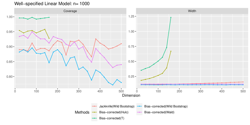
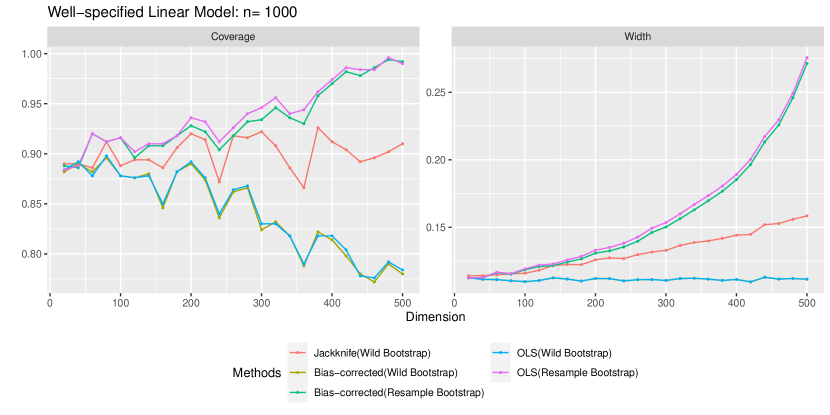
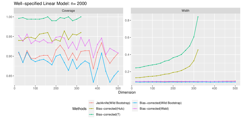
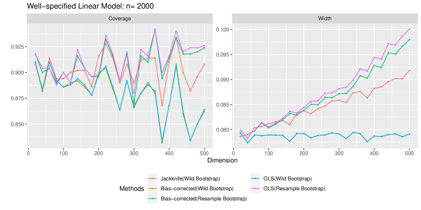
D.2 Additional Figures for Misspecified Model
This section presents the additional numerical results on comparing confidence intervals for the projection parameter under the misspecified model. The simulation settings are summarized in Table 1.
| Figure 5,6 | Figure 7,8 | Figure 9,10 | Figure 11,12 | Figure 13,14 | Figure 15,16 | |
| Figure 17 | Figure 18 | Figure 19 | ||||