Learning Permutation Symmetry
of a Gaussian Vector with gips in R

Adam Chojecki, Paweł Morgen, Bartosz Kołodziejek Learning Permutation Symmetries with gips in R gips: Learning Permutation Symmetries The study of hidden structures in data presents challenges in modern statistics and machine learning. We introduce the gips package in R, which identifies permutation subgroup symmetries in Gaussian vectors. gips serves two main purposes: exploratory analysis in discovering hidden permutation symmetries and estimating the covariance matrix under permutation symmetry. It is competitive to canonical methods in dimensionality reduction while providing a new interpretation of the results. gips implements a novel Bayesian model selection procedure within Gaussian vectors invariant under the permutation subgroup introduced in GIKM, The Annals of Statistics, 50 (3) (2022). Bayesian model selection, permutation symmetry, high-dimensional statistics, dimensionality reduction, parameter sharing, R Bayesian model selection, permutation symmetry, high-dimensional statistics, dimensionality reduction, parameter sharing, R Adam Chojecki, Paweł Morgen, Bartosz Kołodziejek
Warsaw University of Technology
Faculty of Mathematics and Information Science
Koszykowa 75
00-662 Warsaw, Poland
E-mail: , ,

1 Introduction

The study of hidden structures in the data is one of the biggest challenges in modern mathematical statistics and machine learning ElementsOfStatLearn. Extracting meaningful information from high-dimensional datasets, where the number of variables $p$ exceeds the number of observations $n$, poses a significant hurdle due to the curse of dimensionality.

One solution to the problem of an insufficient number of observations relative to the number of variables is to restrict to models with lower dimensionality. Graphical models have been introduced for this purpose L96, where a conditional independence structure (graph Markovian structure) is imposed on the distribution of a random vector. Such structures are conveniently described by graphs and allow for a reduction in the dimensionality of the problem. However, if the graph is not sparse enough, then such a procedure does not allow for a reliable estimation of the covariance matrix. We note that the study of the covariance matrix is the basic way to describe the dependency structure of a random vector and provides a convenient way to quantify the dependencies between variables.

If the data is insufficient and some inference must be performed, one has to propose additional assumptions or restrictions. In such a situation, colored graphical models could be considered, where, in addition to conditional independence, certain equality conditions on the covariance matrix are imposed. Incorporating such equality conditions in colored graphical models is an example of parameter sharing. This concept allows for a reduction of dimensionality and can effectively incorporate domain knowledge into the model architecture. A notable example of parameter sharing, which possesses these advantages, is the convolution technique ElementsOfStatLearn used in image and video processing, enabling efficient feature extraction and pattern recognition.

A rich family of such symmetry conditions can be expressed using the language of permutations. This idea was introduced in AnderssonInvariant; AndersonPermSymmetry and HL08. In the latter paper, three types of such models (RCOP among them) were introduced to describe situations where some entries of concentration or partial correlation matrices are approximately equal. These equalities can be represented by a colored graph. The RCOP model, apart from the graph Markovian structure, permits additional invariance of the distribution with respect to some permutation subgroup. We say that the distribution of a $p$-dimensional random vector $Z$ is invariant under permutation subgroup $\Gamma$ on $V=\{1,\ldots,p\}$ if $Z=(Z_{i})_{i\in V}$ has the same distribution as $(Z_{\sigma(i)})_{i\in V}$ for any permutation $\sigma\in\Gamma$, AnderssonInvariant. This property is called the permutation symmetry of the distribution of $Z$ and imposes significant symmetry conditions on the model.

The case when the conditional dependency graph is unknown or known to be the complete graph was studied in GIKM. In that paper, the authors introduced a Bayesian model selection procedure for the case when $Z$ is a Gaussian vector. In other words, by assuming a prior distribution on the parameters, they derived the posterior probability of a specific model. This allows one to find the permutation group under which (most likely) the data is invariant. Not only does this result in dimensionality reduction but also provides a simple and natural interpretability of the results. For example, if the distribution of $Z$ is invariant under swapping its $i$th and $j$th entries, then one can say that both $Z_{i}$ and $Z_{j}$ play a symmetrical role in the model.

The concept of group invariance finds application in various domains and often leads to improved estimation properties. If the group under which the model is invariant is known, precise convergence rates for the regularized covariance matrix were derived in Shah12, demonstrating significant statistical advantages in terms of sample complexity. Another noteworthy paper, Solo16, explores group symmetries for estimating complex covariance matrices in non-Gaussian models, which are invariant under a known permutation subgroup. However, neither of these articles provides guidance on identifying the permutation subgroup when it is unknown, which is typically the case in practical applications.

Identifying the permutation subgroup symmetry can be interpreted as an automated way of extracting expert knowledge from the data. Discovering the underlying symmetries allows for a deeper understanding of the relationships and dependencies between variables, offering insights that may not be apparent through traditional analysis alone. The automated approach reduces the reliance on manual exploration and expert intervention.

In the present paper, we introduce an R package called gips (acronym derived from ’Gaussian model invariant by permutation symmetry’), gips, which implements the model selection procedure described in GIKM. The gips package, presented in this paper, serves two purposes:

1. Discovering hidden permutation symmetries among variables (exploratory analysis).

2. Estimating covariance matrix under the assumption of known permutation symmetry.

Both points are limited to the Gaussian setting. To the best of our knowledge, there are currently no other software packages available (in R or any other programming language) that address the topic of finding permutation symmetry. Our approach focuses on zero-mean Gaussian vectors, although the method can be applied to centered data and, if the sample size $n$ is reasonably large, to standardized data as well, see Section LABEL:sec:standardizing.

Let $Z$ be a Gaussian vector with a known mean. If we assume full symmetry of the model, see Section 2.2, meaning that the distribution of $Z$ is invariant under any permutation, then the maximum likelihood estimator (MLE) of the covariance matrix requires only a single sample ($n_{0}=1$) to exist. Somewhat surprisingly, the same phenomenon applies when the normal sample is invariant under a cyclic subgroup generated by a cycle of length $p$. While it is natural to consider permutation symmetries alongside conditional independence structures, we follow GIKM and assume no conditional independencies among the variables. Such an approach already enables a substantial reduction in dimensionality, accompanied by a readily interpretable outcome. The development of the method to incorporate non-trivial graph Markovian structures is a topic for future research, and we will consider expanding the package if a new theory emerges. The first step towards generalizing the theory to homogeneous graphs has already been taken in GKI22. Additionally, a simple heuristic can be employed to identify non-trivial Markovian structures using our model - see (GIKM, Section 1.2), (GIKM_SM, Section 4.1), and Section LABEL:sec:brease_cancer in this paper.

Although there are no other software packages available for finding permutation symmetries in data, we have made the decision to compare the results of our model with canonical methods commonly used to tackle high-dimensional problems, namely Ridge and Graphical LASSO (GLASSO) estimation and model selection (implemented, for instance, in R packages: huge huge and rags2ridges rags2ridges; rags2ridges_paper). These methods correspond to estimation with constraints or, conversely, to Bayesian estimation with Gaussian or Laplace priors, respectively (ISL, Sec. 6.2.2). We demonstrate that gips is competitive with these widely used approaches in terms of dimensionality reduction properties, and moreover, it offers interpretability of the results in terms to permutation symmetries.

Furthermore, it is worth noting that due to the discrete nature of the problem, we believe that finding permutation symmetry cannot be adequately addressed by penalized likelihood methods, which are generally much faster than Bayesian methods. Although other methods (which do not have available implementations to our best knowledge) allow for model selection within colored graphical Gaussian models, none of them are applicable to permutation invariant models (RCOP models). Compared to other models (such as RCON, RCOR in HL08, which correspond to different type of restrictions/symmetries), RCOP models possess a more elegant algebraic description and offer a natural interpretation Ge11; GM15; MassamBayesian; Hel20; QXNX21; RRL21.

The “Replication code” is available at https://github.com/PrzeChoj/gips_replication_code.

1.1 Overview of the paper

The paper is organized as follows. The Introduction consists of four subsections. In the next subsection, we present two low-dimensional toy examples that illustrate the use of gips. In the subsequent subsection, we discuss the potential for successfully exploiting group symmetry in many natural real-life problems. In the final subsection of the Introduction, we argue that it is both necessary and sufficient to focus on cyclic symmetries, which are more tractable.

Section 2 provides the necessary methodological background on permutation symmetries and defines the Bayesian model proposed in GIKM, specialized to cyclic subgroups. We also introduce an Markov chain Monte Carlo (MCMC) algorithm that allows the estimation of the maximum a posteriori (MAP) within our Bayesian model, and we discuss the issue of centering and standardizing input data.

Section LABEL:sec:illustrations is dedicated to numerical simulations. We present a high-dimensional example using breast cancer data from Miller. Additionally, we use a heuristic approach from GIKM for identifying the graphical model invariant under permutation symmetries (RCOP model from HL08) and apply this procedure to the real-life example. In the subsequent subsections, we examine the impact of hyperparameters on model selection and compare gips with competing packages that facilitate dimensionality reduction.

Finally, in Section LABEL:sec:summary we draw some conclusions.

An example to Section 1.4 is presented in Appendix LABEL:app:general. Mathematical details behind the Bayesian model are relegated to the Appendix LABEL:app:technical.

1.2 Toy examples

We illustrate the concept of permutation symmetry using the gips package in two simple use cases. These examples demonstrate how permutational symmetry can enhance the data mining process. A similar procedure was successfully applied to the Frets’ heads dataset (GIKM, Section 4.2) and the mathematical marks dataset (GKI22, Section 4).

In the first example, we use aspirin dataset from the HSAUR2 package. By examining the covariance matrix, we manually choose a reasonable permutation symmetry. Additionally, we employ the gips package to demonstrate that our algorithm generates reasonable estimates.

For the second example, we utilize the oddbooks dataset from the DAAG package. We showcase how one can incorporate expert field knowledge in the analysis. We use the gips to find the permutation symmetry and interpret the result.

A standard personal computer (PC) can execute the entire code in this section within $10$ seconds.

1.2.1 Aspirin dataset

This dataset consists of information about a meta-analysis of the efficacy of Aspirin (versus placebo) in preventing death after a myocardial infarct.

We renumber the columns for better readability: R> data("aspirin", package = "HSAUR2") R> Z <- aspirin R> Z[, c(2, 3)] <- Z[, c(3, 2)] R> names(Z) <- names(Z)[c(1, 3, 2, 4)] R> head(Z, 4) dp da tp ta 1 67 49 624 615 2 64 44 771 758 3 126 102 850 832 4 38 32 309 317

Each of the $n=7$ rows in Z corresponds to a different study, and the $p=4$ columns represent the following: dp: number of deaths after placebo, da: number of deaths after Aspirin, tp: total number subjects treated with placebo, ta: total number of subjects treated with Aspirin.

Initially, we calculate the empirical covariance matrix S:

R> n <- nrow(Z) R> p <- ncol(Z) R> S <- cov(Z)

Note that since $n=7$ is greater than $p=4$, S is the standard MLE of $\Sigma$ in the (unrestricted) Gaussian model. The heatmap of the S matrix is shown in Figure 1.

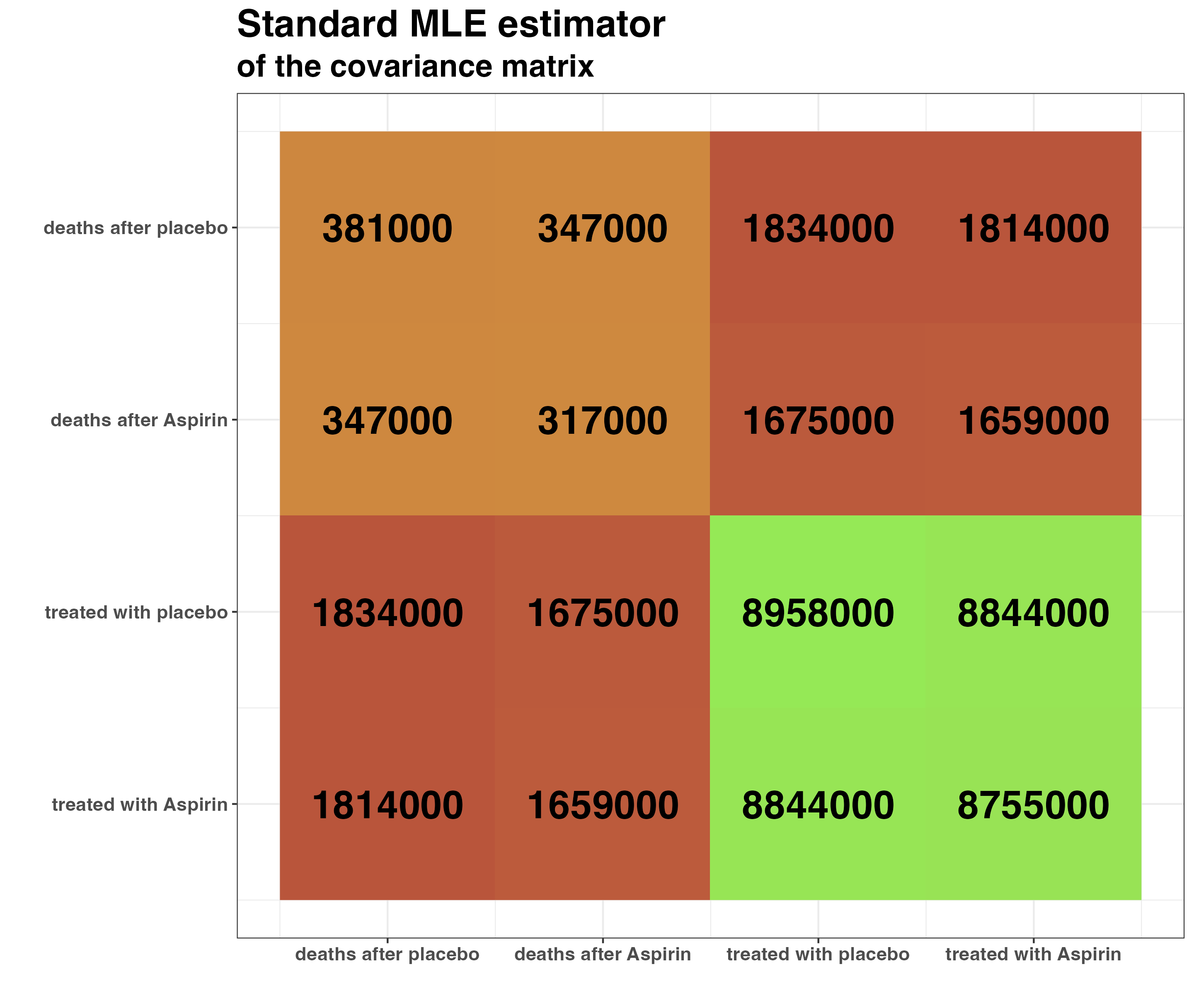
Figure 1: Standard MLE of the covariance matrix of the aspirin dataset. We can see that some entries of S have similar colors, which suggests a lower dimensional model with equality constraints.

We observe significant similarities between the empirical covariances of variables tp (column $3$) and ta (column $4$). They exhibit comparable variances (S[3,3] $\approx$ S[4,4]), and their covariances with the other variables also show resemblance (S[1,3] $\approx$ S[1,4] and S[2,3] $\approx$ S[2,4]).

By definition, the distribution of a random vector $Z=(Z_{1},Z_{2},Z_{3},,Z_{4})^{\top}$ is invariant under the permutation $(3,4)$ if the distributions of $(Z_{1},Z_{2},Z_{3},Z_{4})^{\top}$ and $(Z_{1},Z_{2},Z_{4},Z_{3})^{\top}$ coincide. When $Z$ follows a centered Gaussian distribution, this property can be expressed purely in terms of its covariance matrix, leading to the following conditions: $\VAR[Z_{3}]=\VAR[Z_{4}]$, $\COV[Z_{1},Z_{3}]=\COV[Z_{1},Z_{4}]$, and $\COV[Z_{2},Z_{3}]=\COV[Z_{2},Z_{4}]$. We observe that the structure of S closely corresponds to that of the covariance matrix of a random vector invariant under the permutation $(3,4)$. By observing that S[1,1] $\approx$ S[2,2], S[1,3] $\approx$ S[2,3], and S[1,4] $\approx$ S[2,4], we can also argue that the data is invariant under the permutation $(1,2)$ or even $(1,2)(3,4)$.

We want to emphasize that such manual exploration becomes infeasible for larger values of $p$ due to the massive number and complexity of possible relationships. A priori, it is unclear which scenario is preferable (one can compare Bayesian information criterion (BIC), but the MLE does not always exist). The gips package uses the Bayesian paradigm (described in detail in Section LABEL:sec:BM) to precisely quantify posterior probabilities of considered permutation groups. The workflow in gips is as follows: first, use the gips() function to define an object of the class ‘gips‘ that contains all the necessary information for the model. Next, use the find_MAP() function with an optimizer of your choice to find the permutation that provides the maximum a posteriori estimate. Finally, we use the project_matrix() function to obtain the MLE of the covariance matrix in the invariant model, which will serve as a more stable covariance estimator. The process can be summarized as follows: R> g <- gips(S, n) R> g_MAP <- find_MAP(g, optimizer = "BF", + save_all_perms = TRUE, return_probabilities = TRUE + ) R> g_MAP The permutation (1,2)(3,4): - was found after 17 posteriori calculations; - is 3.374 times more likely than the () permutation. According to the output of find_MAP(), the permutation $(1,2)(3,4)$ best reflects the symmetries of the models and is over $3$ times more probable (under our Bayesian setting) than the identity permutation (), which corresponds to no symmetry. The invariance with respect to the permutation $(3,4)$ arises from the fact that the samples of patients treated with aspirin and placebo had similar sizes. On the other hand, the invariance with respect to the permutation $(1,2)$ signifies the lack of aspirin treatment effect. The permutation $(1,2)(3,4)$ corresponds to both of these effects. We emphasize that this study is an exploratory analysis rather than a statistical test.

We can easily calculate probabilities of all symmetries using a built-in function: R> get_probabilities_from_gips(g_MAP) (1,2)(3,4) (3,4) (1,2) () (1,4) (1,3) 5.107108e-01 1.695605e-01 1.663982e-01 1.513854e-01 4.341644e-04 4.047690e-04 (2,4) (2,3) (1,3,2,4) (1,3)(2,4) (1,4)(2,3) (1,3,4) 3.797581e-04 3.607292e-04 1.240381e-04 7.410652e-05 7.406484e-05 2.197791e-05 (1,2,4) (1,2,3) (2,3,4) (1,2,4,3) (1,2,3,4) 2.026609e-05 1.813565e-05 1.782315e-05 7.676231e-06 7.528912e-06 or compare two permutations of interest: R> compare_posteriories_of_perms(g_MAP, "(34)") The permutation (1,2)(3,4) is 3.012 times more likely than the (3,4) permutation. R> compare_posteriories_of_perms(g_MAP, "(12)") The permutation (1,2)(3,4) is 3.069 times more likely than the (1,2) permutation. R> compare_posteriories_of_perms(g_MAP, "()") The permutation (1,2)(3,4) is 3.374 times more likely than the () permutation.

Note that for $p=4$, there are $p!=24$ different permutations, but only $17$ distinct symmetries are reported above. This is because some permutations correspond to the same symmetry. More precisely, it is the group generated by a permutation $\sigma$ and not $\sigma$ itself that identifies the symmetry. For example $\sigma_{1}=(1,2,3)$ and $\sigma_{2}=(1,3,2)$ generate the same group.

We also note that given the small number of variables ($p=4$), the space of possible permutation symmetries is also small. Consequently, we were able to compute the exact posterior probabilities of our Bayesian model for every single permutation symmetry. The number of permutation symmetries grows superexponentially with $p$, e.g., for $p=10$ its cardinality is approximately $1$ million (see OEIS sequence A051625). Thus, for larger $p$ we recommend using the implemented Metropolis-Hastings algorithm to approximate these probabilities, see Section LABEL:sec:search.

Assuming that the data actually come from a distribution invariant under the permutation $(1,2)(3,4)$, we can provide a new estimate for the covariance matrix. Formally, we project the matrix S onto the space of positive definite matrices that are invariant under the permutation $(1,2)(3,4)$ (for further details, refer to Section 2.3). In practice, we enforce the desired equalities by averaging. R> S_projected <- project_matrix(S, g_MAP) One can easily plot the found covariance estimator with a line: R> plot(g_MAP, type = "heatmap") It is shown in Figure 2 (we made cosmetic modifications to this plot; the exact code is provided in the attached “Replication code”).

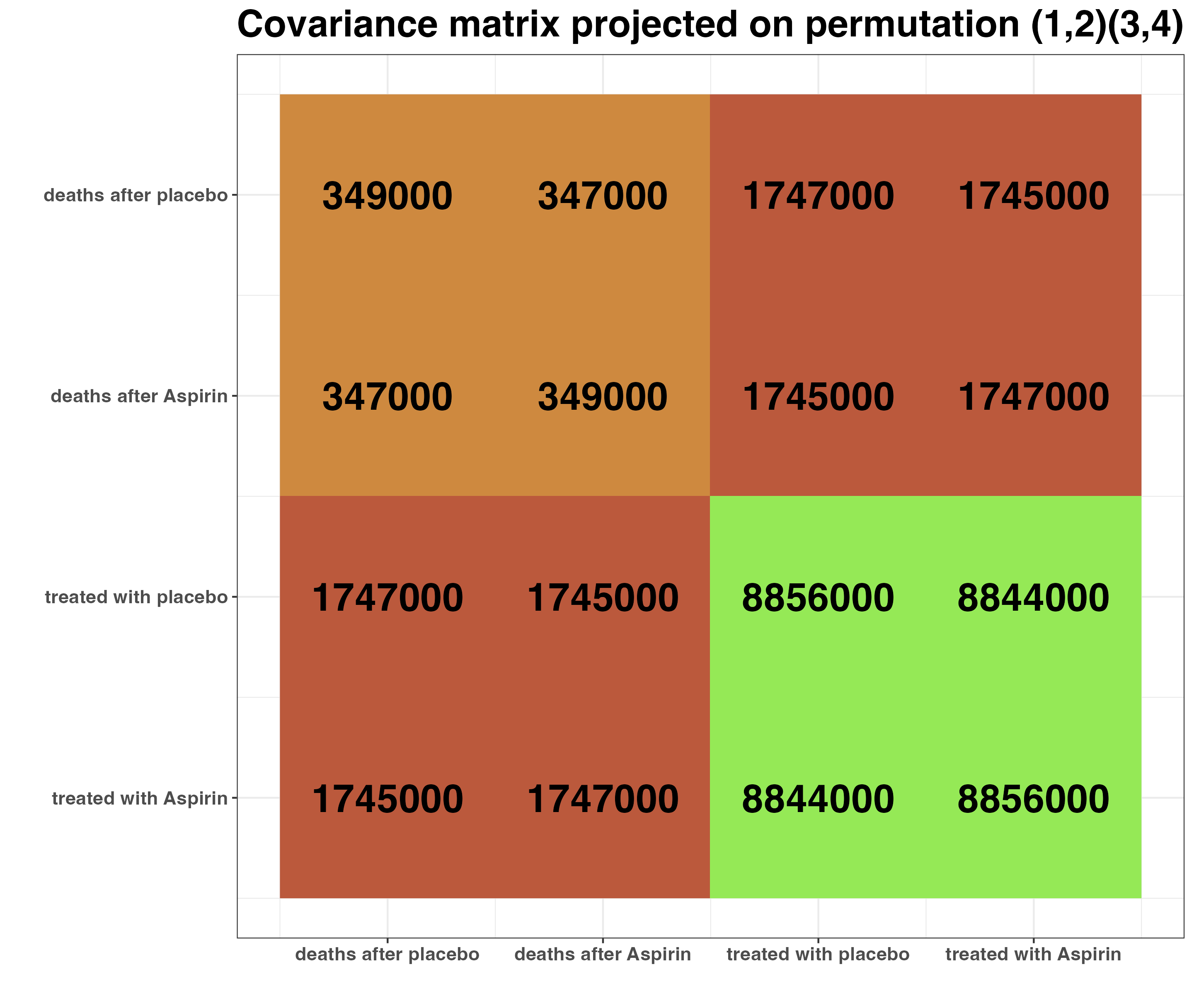
Figure 2: The MLE of the covariance matrix of the oddbooks dataset in the model invariant under the permutation $(1,2)(3,4)$. We can see that the entries corresponding to similar colors in Figure 1 are exactly equal.

The S_projected matrix can now be interpreted as a more stable covariance matrix estimator, see e.g., Shah12; Solo16.

1.2.2 Books dataset

This dataset consists of information about thickness (mm), height (cm), width (cm), and weight (g) of $12$ books.

R> data("oddbooks", package = "DAAG") R> head(oddbooks, 4) thick height breadth weight 1 14 30.5 23.0 1075 2 15 29.1 20.5 940 3 18 27.5 18.5 625 4 23 23.2 15.2 400

We will only consider relationships between the thickness, height, and width. R> Z <- oddbooks[, c(1, 2, 3)]

One can suspect that books from this dataset were printed with a $\sqrt{2}$ aspect ratio, as in the popular A-series paper size. Therefore, we can utilize this domain knowledge in the analysis and unify the data for height and width: R> Z$height<-Z$height / sqrt(2)

Let us see the standard MLE of the covariance matrix: R> S <- cov(Z) We can plot this covariance matrix to see if we would notice any connection between variables. Figure 3 was obtained with the code below (we made cosmetic modifications to this plot; the exact code is provided in the attached “Replication code”):

R> g <- gips(S, number_of_observations) R> plot(g, type = "heatmap")

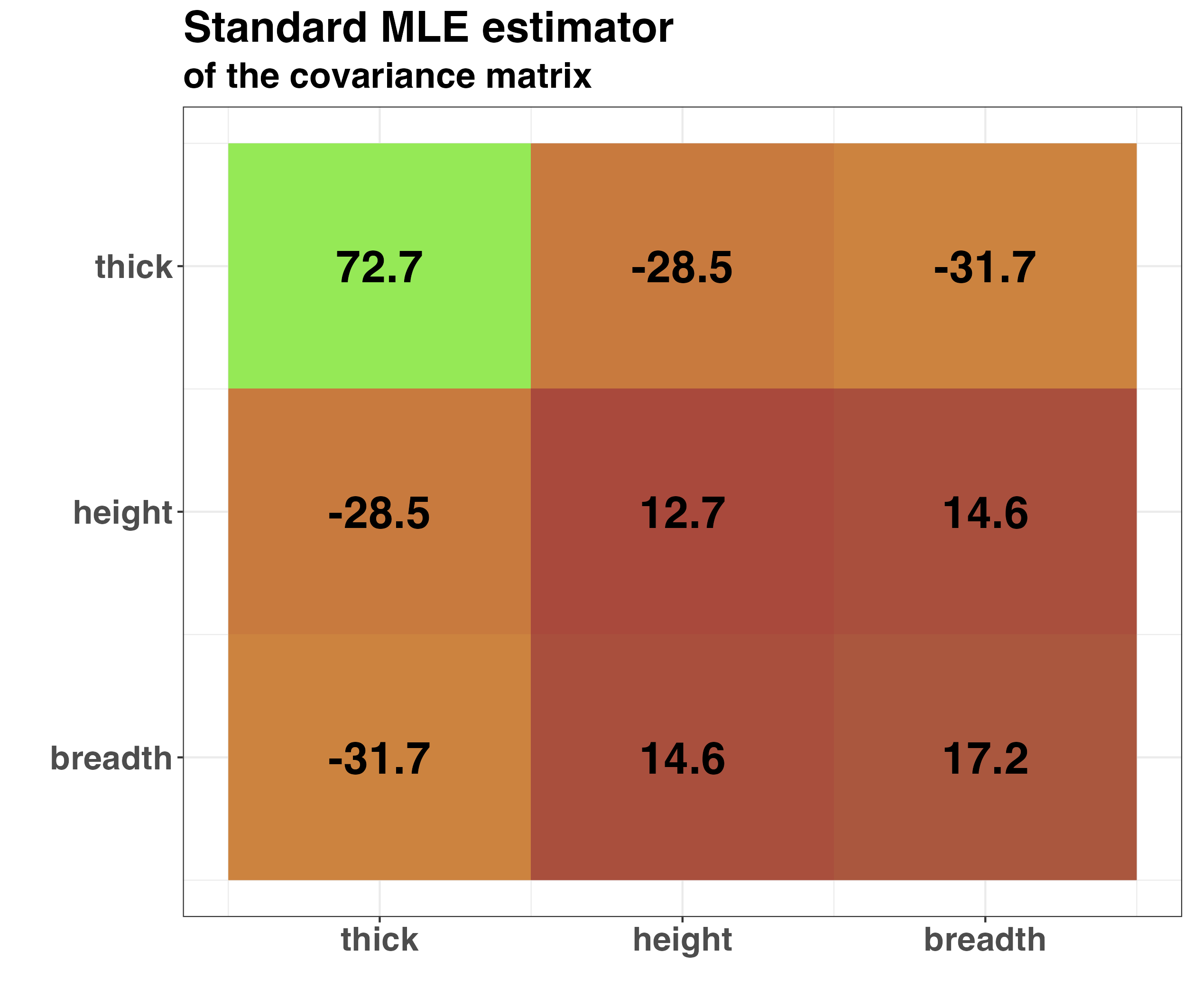
Figure 3: Standard MLE of the covariance matrix of the oddbooks dataset. We can see that some entries of S have similar colors, which suggests a lower dimensional model with equality constraints.

We can see that some entries of S have similar colors, which suggests a lower dimensional model with equality constraints. In particular, the covariance between thick and height is very similar to the covariance between thick and breadth, and the variance of height is similar to the variance of breadth. Those are not surprising, given the data interpretation (after the height rescaling that we did).

Let us examine the posterior probabilities returned by gips: R> g_MAP <- find_MAP(g, optimizer = "BF", + return_probabilities = TRUE, save_all_perms = TRUE + ) R> get_probabilities_from_gips(g_MAP) (2,3) () (1,3) (1,2,3) (1,2) 5.660781e-01 4.339087e-01 6.728772e-06 4.683290e-06 1.862353e-06

We see that the a posteriori distribution is maximized by a permutation (2,3). The MLE of the covariance matrix in the model invariant under the permutation (2,3) is presented in Figure 4.

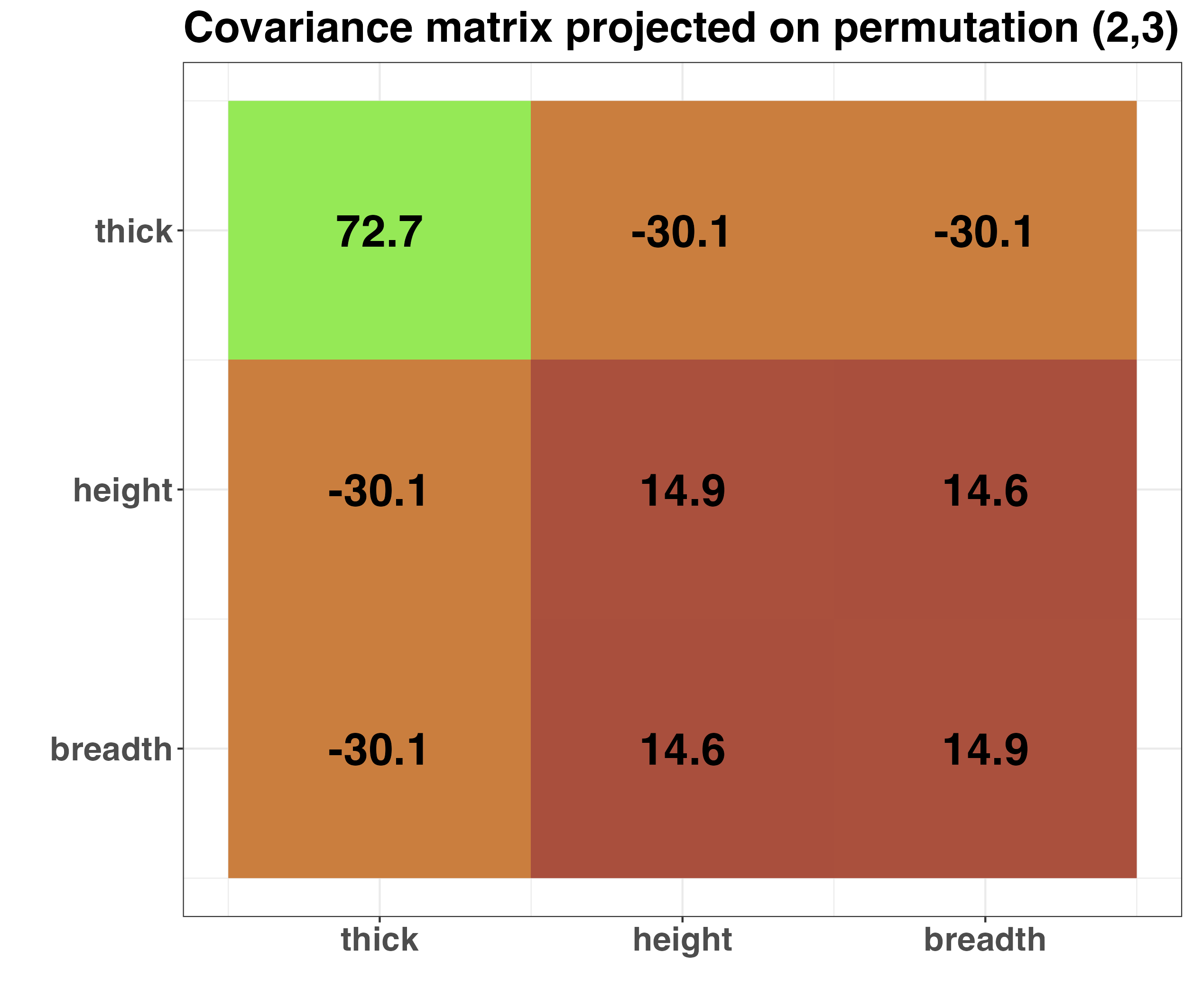
Figure 4: Estimator of the covariance matrix of the oddbooks dataset after the projection on the permutational symmetry group (2,3). We can see that now similar colors from Figure 3 are exactly equal.

1.3 Motivation behind permutation symmetries

We argue that it is natural to expect certain symmetries in various applications, which strengthens the need for tools to investigate permutation symmetry within the data.

For example, there are natural symmetries in the data from gene expression. Specifically, the expression of a given gene is triggered by the binding of transcription factors to gene transcription factor binding sites. Transcription factors are proteins produced by other genes, often referred to as regulatory genes. Within the gene network, it is common for multiple genes to be triggered by the same regulatory genes, suggesting that their relative expressions depend on the abundance of the regulatory proteins (i.e., gene expressions) in a similar manner GIKM. Extracting permutation symmetries can be utilized to identify genes with similar functions or groups of genes with similar interactions or regulatory mechanisms. This approach is particularly useful in unraveling the structures of gene regulatory networks KE20.

Furthermore, in examples of social networks, such as those influenced by geographical or social group clusters, additional symmetries must be taken into account, as mentioned in GM15. In the study of the human brain’s dynamics, it is believed that the left and right hemispheres possess a natural symmetric structure RRL21.

The discovery of hidden symmetries can greatly contribute to understanding complex mechanisms. Extracting patterns from gene expression profiles can offer valuable insights into gene function and regulatory systems TH02. Clustering genes based on their expression profiles can aid in predicting the functions of gene products with unknown purposes and identifying sets of genes regulated by the same mechanism.

1.4 Arbitrary permutation symmetries vs cyclic permutation symmetries

As observed in GIKM, performing model selection within an arbitrary permutation subgroup is a highly challenging task. This difficulty arises not only due to theoretical reasons but also because of computational complexity issues arising when $p$ is large. Informally speaking, finding the parameters of an arbitrary permutation group becomes virtually impossible for large values of $p$. In GIKM, a general model was developed; however, it was specifically applied to cyclic subgroups. Such subgroups are generated by a single permutation, and by restricting the analysis to them, efficient methods can be devised to conduct the model selection procedure. All the technical details regarding these methods will be presented in the subsequent sections.

Furthermore, we argue that cyclic subgroups form a sufficiently rich family, as mentioned in (GIKM, Section 4.1). Since these subgroups correspond to simpler symmetries, they are also more easily interpretable. Although our procedure exclusively explores cyclic subgroups, it can still provide valuable information even when the true subgroup is not cyclic, as discussed in (GIKM_SM, Section 3.3). In fact, if the posterior probabilities (which are calculated with gips) are high for multiple groups, it is reasonable to expect that the data will exhibit invariance under the group containing those subgroups. We present a simple example in the Appendix LABEL:app:general.

2 Methodological background

After providing an informal introduction, let us proceed to define the key concepts and present the theory behind the gips package in a formal manner. Definitions in this section are accompanied with code in gips package. The running example is for $p=5$ and $n=10$. A standard PC can execute all the code in this section within $20$ seconds (except for the final chunk of code in Section LABEL:sec:search which runs for $2$ minutes).

R> p <- 5; n <- 10

2.1 Permutations

Fix $p\in\{1,2,\ldots\}$. Let $\mathfrak{S}_{p}$ denote the symmetric group, the set of all permutations on the set $V=\{1,\ldots,p\}$, with function composition as the group operation.

Each permutation $\sigma\in\mathfrak{S}_{p}$ can be represented in a cyclic form. For example, if $\sigma$ maps $1$ to $2$, $2$ to $1$, and leaves $3$ unchanged, then we can express $\sigma$ as $(1,2)(3)$. It is sometimes convenient to exclude cycles of length $1$ from this representation. The identity permutation is denoted as $\mathrm{id}$ or $()$. The number of cycles denoted as $C_{\sigma}$, remains the same across different cyclic representations of $\sigma$. It is important to note that cycles of length $1$ are included when calculating $C_{\sigma}$.

We say that a permutation subgroup $\Gamma\subset\mathfrak{S}_{p}$ is cyclic if $\Gamma=\{\sigma,\sigma^{2},\ldots,\sigma^{N}\}=:\left<\sigma\right>$ for some $\sigma\in\mathfrak{S}_{p}$, where $N$ is the smallest positive integer such that $\sigma^{N}=\mathrm{id}$. Then, $N$ is the order of the subgroup $\Gamma$. If $p_{i}$ denotes the length of the $i$th cycle in a cyclic decomposition of $\sigma\in\mathfrak{S}_{p}$, then $N$ is equal to the least common multiple of $p_{1},p_{2},\ldots,p_{C_{\sigma}}$.

If $\Gamma=\left<\sigma\right>$, then we say that $\sigma$ is a generator of $\Gamma$. It is worth noting that a cyclic subgroup may have several generators. Specifically, $\left<\sigma\right>=\langle\sigma^{k}\rangle$ for all $k=1,\ldots,N-1$, where $k$ is coprime with $N$. We identify each cyclic permutation subgroup by its generator, which is the smallest permutation according to lexicographic order. For further topics on permutation groups, readers may refer to Alg.

2.2 Permutation symmetry

Let $\Gamma$ be an arbitrary subgroup of $\mathfrak{S}_{p}$. We say that the distribution of $Z=(Z_{i})_{i\in V}$ is invariant under a subgroup $\Gamma$ if $Z$ has the same distribution as $(Z_{\sigma(i)})_{i\in V}$ for all $\sigma\in\Gamma$. If $Z$ is a multivariate random variable following a centered Gaussian distribution $\mathrm{N}_{p}(0,\Sigma)$, then this invariance property can be expressed as a condition on the covariance matrix. Specifically, the distribution of $Z$ is invariant under $\Gamma$ if and only if for all $i,j\in V$:

$$\Sigma_{ij}=\Sigma_{\sigma(i)\sigma(j)}\quad\text{for all}\quad\sigma\in\Gamma.$$ (1)

When $\Gamma=\mathfrak{S}_{p}$, the above conditions imply that all diagonal entries of $\Sigma$ are the same, and similarly, the off-diagonal entries are the same (see the top left panel of Figure 5). On the other hand, if $\Gamma$ is the trivial subgroup, i.e., $\Gamma=\{\mathrm{id}\}$, then (1) does not impose any restrictions on the entries of $\Sigma$. If $\Gamma$ is non-trivial, the sample size $n$ required for the MLE to exist is lower than $p$, as discussed in Section 2.3.

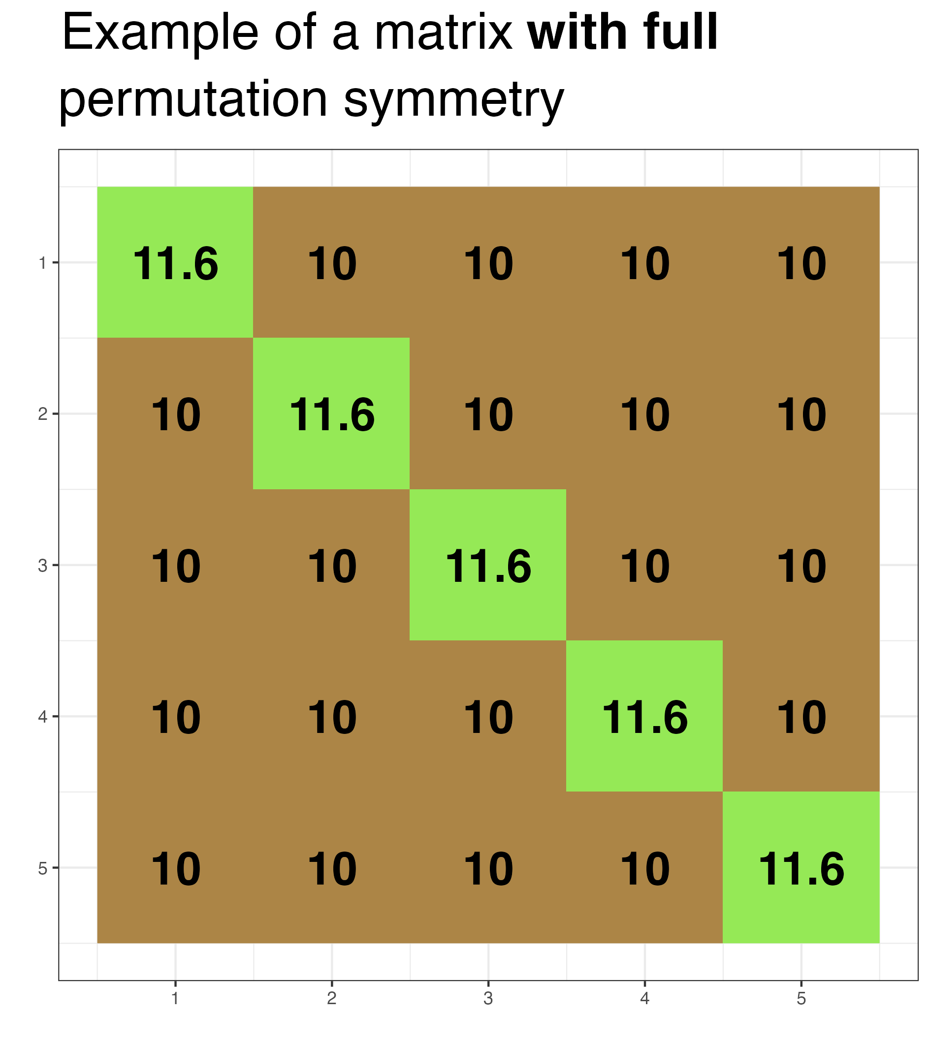
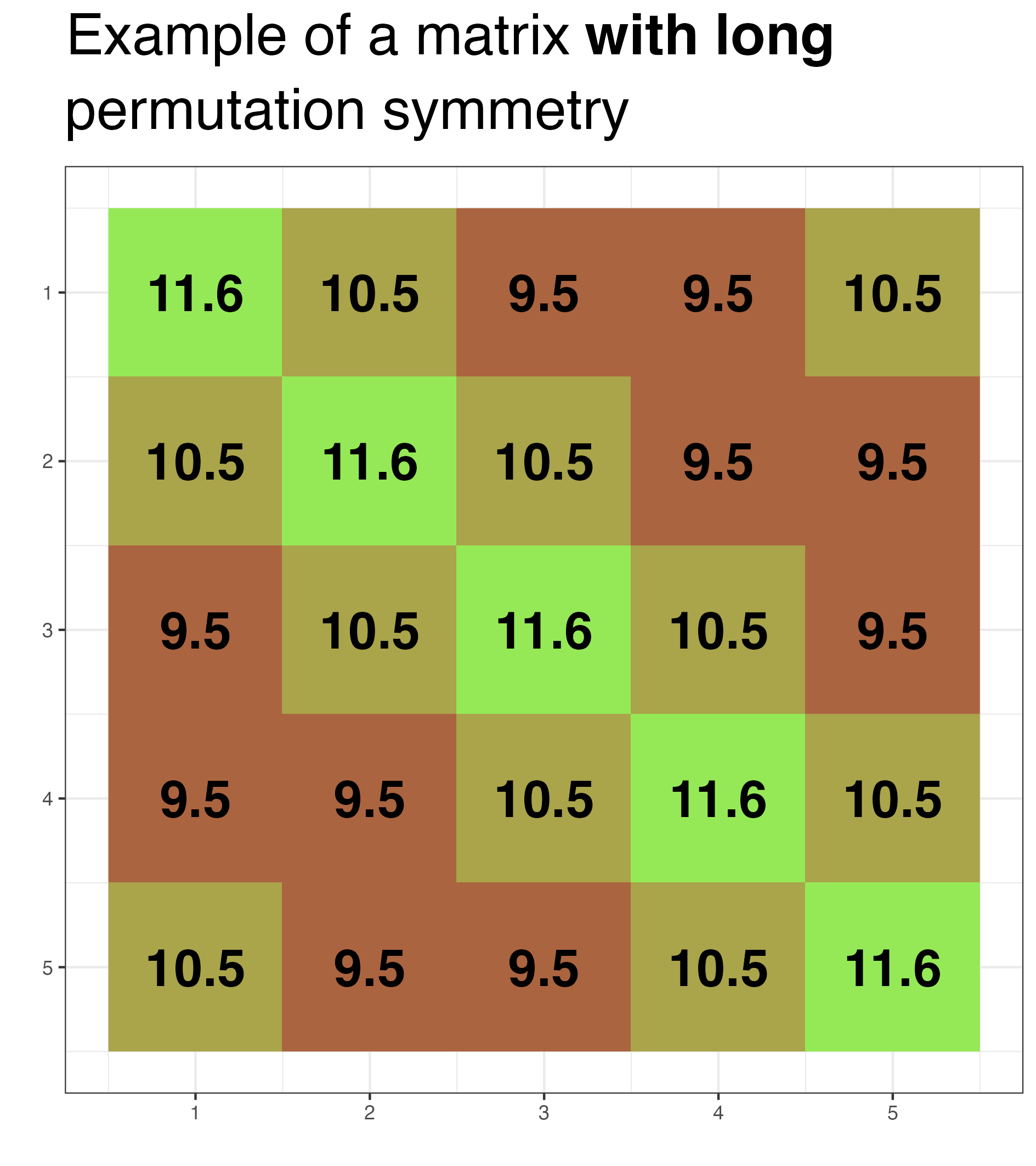
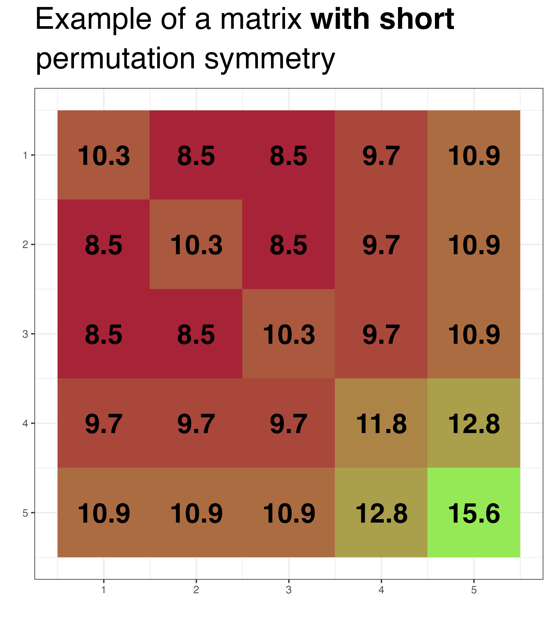
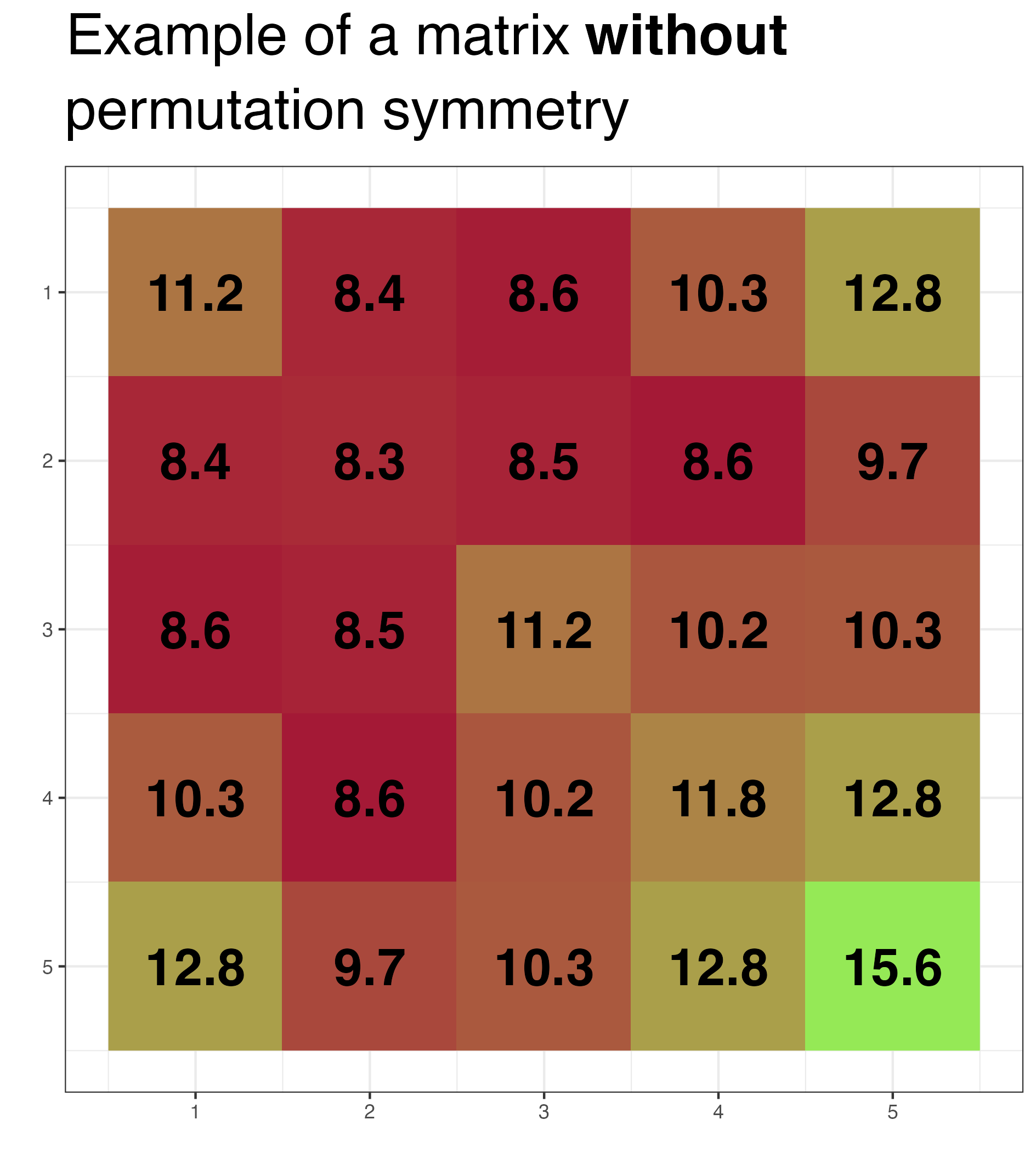
Figure 5: Examples of covariance matrices with symmetries: full $\Gamma=\mathfrak{S}_{p}$ permutation symmetry (top left), long permutation symmetry $\Gamma=\left<(12345)\right>$ (top right), short permutation symmetry $\Gamma=\left<(123)\right>$ (bottom left), no permutation symmetry (bottom right). They all are projections of the same matrix on corresponding colored spaces.

Let $\mathrm{Sym}(p;\mathbb{R})$ and $\mathrm{Sym}^{+}(p;\mathbb{R})$ denote the space of $p\times p$ symmetric matrices and the corresponding cone of positive definite matrices, respectively. For a subgroup $\Gamma\subset\mathfrak{S}_{p}$, we define the colored space as the space of symmetric matrices invariant under $\Gamma$:

$$\mathcal{Z}_{\Gamma}:=\{S\in\mathrm{Sym}(p;\mathbb{R})\colon S_{ij}=S_{\sigma(i)\sigma(j)}\mbox{ for all }\sigma\in\Gamma\},$$

We also define the colored cone of positive definite matrices valued in $\mathcal{Z}_{\Gamma}$ as:

$$\mathcal{P}_{\Gamma}:=\mathcal{Z}_{\Gamma}\cap\mathrm{Sym}^{+}(p;\mathbb{R}).$$

The set $\mathcal{P}_{\Gamma}$ contains all possible covariance matrices of Gaussian vectors invariant under subgroup $\Gamma$. The dimension of the space $\mathcal{Z}_{\Gamma}$ corresponds to the number of free parameters in the covariance matrix. The dependence structure of a Gaussian vector is fully described by the covariance matrix $\Sigma$. When certain entries of $\Sigma$ are identical, we refer to them as having the same color. There are colors that correspond to equalities among the diagonal elements of $\Sigma$, and there are independent colors that correspond to equalities among the off-diagonal elements of $\Sigma$. Thus, in the context of colored models, $\dim(\mathcal{Z}_{\Gamma})$ can be interpreted as the number of distinct colors.

In gips, we can easily find the number of free parameters in the model invariant under a cyclic subgroup as follows (S is a matrix from the bottom right of Figure 5): R> g <- gips(S, n, perm = "(12345)", was_mean_estimated = FALSE) R> summary(g)$n_{p}arameters\CodeOutput 3\par Noticetherewereexactly$3$differentnumbersinthematrixfromthetoprightofFigure~{}\ref{fig:example_symmetries}.\par Itisimportanttonotethatthemapping$Γ↦Z_Γ$isnotone-to-one.Inparticular,for$p=3$,wehave$Z_⟨(1,2,3)⟩=Z_S_3$.Anotablepropertyofcyclicsubgroupsisthattheycorrespondtodifferentcoloredspaces.Moreprecisely,if$Z_⟨σ⟩=Z_⟨σ’⟩$forsome$σ,σ’∈S_p$,then$⟨σ⟩=⟨σ’⟩$\cite[cite]{(\@@bibref{AuthorsPhrase1Year}{GIKM}{\@@citephrase{, }}{}, Lemma 15)}.\par\par$

2.3 The MLE in the Gaussian model invariant under permutation symmetry

Let $Z^{(1)},\ldots,Z^{(n)}$ be an independent and identically distributed (i.i.d.) sample from $\mathrm{N}_{p}(0,\Sigma)$. The presence of equality restrictions in (1) reduces the number of parameters to estimate in permutation invariant models. Consequently, the sample size required for the MLE of $\Sigma$ to exist is lower than $p$ for non-trivial subgroup $\Gamma\subset\mathfrak{S}_{p}$. Assuming $\Sigma\in\mathcal{P}_{\Gamma}$, where $\Gamma=\left<\sigma\right>$ is a cyclic subgroup, (GIKM, Corollary 12) establishes that the MLE of $\Sigma$ exists if and only if

$$n\geq n_{0}:=C_{\sigma}.$$ (2)

In particular, when $\sigma=\mathrm{id}$, no restrictions are imposed on $\Sigma$, and we recover the well-known condition that the sample size $n$ must be greater than or equal to the number of variables $p=C_{\mathrm{id}}$. However, if $\sigma$ consists of a single cycle, i.e., $C_{\sigma}=1$, the MLE always exists. This remarkable observation is crucial in high-dimensional settings.

In gips, we can compute $n_{0}$ as follows: R> g <- gips(S, n, perm = "(12345)", was_mean_estimated = FALSE) R> summary(g)$n0\CodeOutput 1\CodeInput R>g<-gips(S,n,perm="()",was_{m}ean_{e}stimated=FALSE)R>summary(g)$n0\CodeOutput 5\par If(\ref{eq:n0})issatisfied,theMLEof$Σ$isgivenby$$\hat{\Sigma}=\pi_{\Gamma}\left(\frac{1}{n}\sum_{i=1}^{n}Z^{(i)}\cdot(Z^{(i)})^{\top}\right),$$where$π_Γ$denotestheorthogonalprojectionontothecoloredspace$Z_Γ$.Itisisdefinedas\begin{aligned} \pi_{\Gamma}(X)=\frac{1}{\#\Gamma}\sum_{\sigma\in\Gamma}\sigma\cdot X\cdot\sigma^{\top},\end{aligned}whereeachpermutation$σ$isidentifiedwithitscorrespondingpermutationmatrix.Theresultingmatrix$π_Γ(X)$isoftenreferredtoastheregularizedmatrixsincethemappingaveragestheentriesof$X$thatcorrespondtothesameorbitsof$Γ$:for${i,j}⊂V$defineits$Γ$-orbitby$O_ij^Γ={ {σ(i),σ(j)}:σ∈Γ}$.Then,forany${u,v}∈O_ij^Γ$onehas\begin{aligned} \pi_{\Gamma}(X)_{uv}=\frac{1}{\#O_{ij}^{\Gamma}}\sum_{\{k,l\}\in O_{ij}^{\Gamma}}X_{kl}.\end{aligned}\par In\pkg{gips},theprojection$π