A Monte Carlo Policy Gradient Method with Local Search for Binary Optimization

Abstract

Binary optimization has a wide range of applications in combinatorial optimization problems such as MaxCut, MIMO detection, and MaxSAT. However, these problems are typically NP-hard due to the binary constraints. We develop a novel probabilistic model to sample the binary solution according to a parameterized policy distribution. Specifically, minimizing the KL divergence between the parameterized policy distribution and the Gibbs distributions of the function value leads to a stochastic optimization problem whose policy gradient can be derived explicitly similar to reinforcement learning. For coherent exploration in discrete spaces, parallel Markov Chain Monte Carlo (MCMC) methods are employed to sample from the policy distribution with diversity and approximate the gradient efficiently. We further develop a filter scheme to replace the original objective function by the one with the local search technique to broaden the horizon of the function landscape. Convergence to stationary points in expectation of the policy gradient method is established based on the concentration inequality for MCMC. Numerical results show that this framework is very promising to provide near-optimal solutions for quite a few binary optimization problems.

1 Introduction

In this paper, we consider the following binary optimization problem:

$$\min_{x}\quad f(x),\quad\text{s.t. }\quad x\in\mathcal{B}_{n},$$ (1)

where $\mathcal{B}_{n}=\{-1,1\}^{n}$ represents the binary set of dimension $n$ and $f$ can be any function defined on $\mathcal{B}_{n}$. Binary optimization (1) is a classical form of optimization with a wide range of practical applications, including the MaxCut problem, the quadratic 0-1 programming problem, the Cheeger cut problem, the MaxSAT problem, and the multiple-input multiple-output (MIMO) detection problem. Obtaining the optimal solution for these problems is typically NP-hard due to the nature of binary constraints. Therefore, exact methods, such as branch-and-bound land1960automatic and cutting plane gilmore1961linear designed for linear integer programming, hardly work for general large-scale binary problems. Moreover, the objective function $f$ in (1) may be quite complicated, adding difficulties in finding the global optimum.

Approximate algorithms based on relaxation sacrifice optimality to find high-quality solutions. For binary quadratic problems, semidefinite programming (SDP) provides a relaxation of the primal problem and achieves near optimal solutions with the particular rounding schemewai2011cheap ; burer2001projected . This becomes a paradigm to solve the binary optimization problem with quadratic objective function. MADAM solves MaxCut based on SDP and ADMM hrga2021madam . EMADM provides an entropy regularized splitting model for the SDP relaxation on the Riemannian manifold liu2022entropy . BiqCrunch incorporates an efficient SDP-based bounding procedure into the branch-and-bound methodkrislock2017biqcrunch . Solving the dual problem of SDP relaxation is also utilized for the MaxCut problem rendl2010solving ; krislock2014improved , which can be further efficiently solved by a customized coordinate ascent algorithm buchheim2019sdp .

Heuristic methods is the another way to provide a good solution for the problem within a reasonable time frame, but do not have a reliable theoretical guarantees in most cases. One of the classical heuristic methods is simulated annealing, which is developed to find a good solution by iteratively swapping variables between feasible and infeasible points with a probability that depends on the measurement called “temperature” eglese1990simulated ; kirkpatrick1983optimization ; aarts1989simulated . Greedy algorithm is the another type of heuristic methods that makes the locally optimal choice at each step and is applied on the traveling salesman problem gutin2006traveling , the minimum spanning tree problem prim1957shortest and etc. A typical greedy method is local search, which explores the search space in the neighborhood of the current solution and selects the best neighboring solution baum1987towards ; martin1991large ; mladenovic1997variable ; johnson1997traveling .

In recent years, there has been a growing interest in applying machine learning methods to solve combinatorial optimization problems. The early work was based on pointer networksvinyals2015pointer , which leverage sequence-to-sequence models to produce permutations over inputs of variable size, as is relevant for the canonical travelling salesman problem (TSP). Since then, numerous studies have fused GNNs with various heuristics and searching procedures to solve specific combinatorial optimization problems, such as graph matchingbai2019simgnn , graph colouringlemos2019graph and the TSPli2018combinatorial . Recent works aim to train neural networks in an unsupervised, end-to-end fashion, without the need for labelled training sets. Specifically, RUN-CSPtoenshoff2019run solves optimization problems that can be framed as maximum constraint satisfaction problems. In yao2019experimental ; karalias2020erdos , a GNN is trained to specifically solve the MaxCut problem on relatively small graph sizes with up to 500 nodes.

1.1 Our contributions

In this work, we propose an efficient and stable framework, called Monte Carlo policy gradient (MCPG), to solve binary optimization problems by stochastic sampling. Our main contributions are summarized as follows.

• A novel probabilistic approach. We first construct a probabilistic model to sample binary solutions from a parameterized policy distribution. While the Gibbs distribution can locate optimal binary solutions, it suffers from high computational complexity of sampling for a complicated function. Therefore, we introduce a parameterized policy distribution with improved sampling efficiency and a stochastic optimization problem is obtained by minimizing the KL divergence between the parameterized policy distribution and the Gibbs distributions. Due to the parameterization on the distribution, an explicit formulation of the gradient can be derived similarly to the policy gradient in reinforcement learning. Consequently, a policy gradient method with stochastic sampling is applied to find the parameters of the policy distribution and the parameterized policy distribution can guide us to search for high-quality binary solutions.

• An efficient parallel sampling scheme. Instead of direct sampling, we employ a parallel MCMC method to sample from the policy distribution and compute the policy gradient with MCMC samples. The parallel MCMC method takes advantage of both high-quality initialization and massive parallelism. The Markov property of samples maintains consistency of the sampling process and the parallelization enables a wide range of exploration for binary solutions. A filter function is further developed in sampling to flatten the original binary optimization problem within a neighborhood. Based on local search methods, the filter technique improves the quality of binary solutions and reduces the potential difficulty to deal with the functions in discrete spaces.

• Theoretical guarantees for near-optimal solutions. First, the probabilistic model with a smaller expectation of the function value is shown to have a higher probability for sampling optimal points. Then, we demonstrate that the filter function may lead to smaller function values with high probability. Using the concentration inequality of Markov chains, it is proven that the policy gradient method converges to stationary points in expectation. These results partly explain why our method can provide near-optimal solutions with efficiency and stability.

• A simple yet practical implementation. Our algorithm can outperform other state-of-the-art algorithms in terms of solution quality and efficiency on quite a few problems such as MaxCut, MIMO detection, and MaxSAT. Specifically, for the MaxCut problem, MCPG achieves better solutions than all previously reported results on two instances of the public dataset Gset, indicating that MCPG can find optimal solutions.

Additionally, our approach can also be extended to solve the general constrained binary optimization problem:

$$\min_{x}\quad f(x),\;\text{s.t. }\;c(x)=0,\;x\in\mathcal{B}_{n},$$ (2)

where $c(x)=(c_{1}(x),\ldots,c_{m}(x))^{\top}\in\mathbb{R}^{m}$.

1.2 Comparison with Other Probabilistic Methods

Sampling the binary solution from well-designed distribution is not rare in solving binary optimization problems. For example, the Goemans-Williamson (GW) algorithm goemans1995improved uses the randomized rounding technique in solving binary quadratic problems based on semidefinite relaxation. Since the SDP solution can be decomposed as $X=V^{T}V$ where $V=[v_{1},\dots,v_{n}]$ with $v_{i}$ on the unit sphere, the $i$-th component of the binary solution is obtained by taking the sign of the inner product between $v_{i}$ and a random vector $r$ uniformly on the sphere. It has been proven that the GW algorithm has a $0.878$ approximate rate on the MaxCut and Max2SAT problems goemans1995improved ; goemans1994879 . From then on, variants of the GW algorithm have been proposed for MIMO detection problems mobasher2007near ; jiang2021tightness and MaxCut problems krislock2014improved ; rendl2010solving . While the sampling distribution is fixed in the GW algorithm for randomized rounding, our parameterized distribution is refined iteratively in the policy gradient procedure.

Many learning methods for combinatorial optimization also appears with probabilistic methods. Erdos karalias2020erdos is one of the typical learning methods, which proposes an unsupervised learning approach for combinatorial optimization problems on graphs. It utilizes the distribution over nodes parameterized by a graph neural network and performs mini-batch gradient descent to a probabilistic penalty loss function. Many of the unsupervised learning algorithms have similar framework as Erdos. PI-GNN schuetz2022combinatorial applys a differentiable loss function based on the relaxation strategy to the problem Hamiltonian, where the probability over nodes is also represented by a graph neural network. They sample directly from the distribution over nodes and generate binary solutions with an extra decoding step. Distinguished from these methods, we establish an entropy-regularized probabilistic model with a parameterized sampling policy and employ a MCMC sampling algorithm to keep the consistency among the binary solutions.

1.3 Organization

The rest of this paper is organized as follows. In Section 2, we propose a probabilistic model and adopt a policy gradient method. Then, a universal prototype algorithm is given. In Section 3, we modify our MCPG framework with a filter function. In Section 4, we investigate theoretical results on the local search technique and the convergence of MCPG. Numerical experiments on various problems are reported in Section 5. Finally, we conclude the paper in Section 6.

2 Probabilistic model for binary optimization

In this section, we will build the probabilistic model for solving binary optimization problems. A discussion that optimal points can be found by Gibbs distributions is first presented. It motivates us to introduce an extra parameterized policy distribution as an approximation of Gibbs distributions. We construct the objective function by minimizing the KL divergence between these two distributions. The mean field (MF) approximation is used to reduce the complexity of our model. Finally, we describe a policy gradient method to find the optimal sampling policy.

2.1 Parameterized probabilistic model

Since binary optimization problem (1) is typically NP-hard, finding a point $x$ of high quality poses a significant challenge. The goal is to search for the set of optimal points $\mathcal{X}^{*}$ in the discrete space $\mathcal{B}_{n}$, where continuous optimization algorithms cannot operate directly. A probabilistic approach is to consider an indicator distribution, i.e.,

$$q^{*}(x)=\frac{1}{|\mathcal{X}^{*}|}\mathbbm{1}_{\mathcal{X}^{*}}(x)=\begin{cases}\frac{1}{|\mathcal{X}^{*}|},&\quad x\in\mathcal{X}^{*},\\ 0,&\quad x\not\in\mathcal{X}^{*}.\end{cases}$$

The distribution $q^{*}$ is the ideal distribution where only the optimal points have the uniform probability. However, the optimal points set $\mathcal{X}^{*}$ is unknown. To approach $q^{*}$, we introduce the following family of Gibbs distributions:

$$q_{\lambda}(x)=\frac{1}{Z_{\lambda}}\exp\left(-\frac{f(x)}{\lambda}\right),\quad x\in\mathcal{B}_{n},$$ (3)

where $Z_{\lambda}=\sum_{x\in\mathcal{B}_{n}}\exp\left(-\frac{f(x)}{\lambda}\right)$ is the normalization factor. Given the optimal value $f^{*}$ of the objective function, for any $x\in\mathcal{B}_{n}$, we notice that

$$q_{\lambda}(x) =\frac{\exp\left(\frac{f^{*}-f(x)}{\lambda}\right)}{\sum_{x\in\mathcal{B}_{n}}\exp\left(\frac{f^{*}-f(x)}{\lambda}\right)}=\frac{\exp\left(\frac{f^{*}-f(x)}{\lambda}\right)}{|\mathcal{X}^{*}|+\sum_{x\in\mathcal{B}_{n}/\mathcal{X}^{*}}\exp\left(\frac{f^{*}-f(x)}{\lambda}\right)}$$ (4)

$$\to\frac{1}{|\mathcal{X}^{*}|}\mathbbm{1}_{\mathcal{X}^{*}}(x),\quad\text{as }\lambda\to 0.$$

Although $q^{*}$ is not computable in practice, the Gibbs distribution $q_{\lambda}$, which converges to $q^{*}$ pointwisely, provides a feasible alternative for searching optimal solutions.

Motivated by this observation, one can devise an algorithm to randomly sample from the Gibbs distribution and control the parameter $\lambda$ to approximate the global optimum. However, since $q_{\lambda}(x)$ needs to compute the summation of $2^{n}$ terms in the denominator $Z_{\lambda}$, the complexity of direct sampling grows exponentially. Meanwhile, $q_{\lambda}$ is hard to sample when $f$ owns a rough landscape. Instead of direct sampling from the Gibbs distribution, we approximate it using a parameterized policy that can be sampled efficiently. The parameterized distribution $p_{\theta}(x|\mathcal{P})$ is designed to have a similar but regular landscape to that of $q_{\lambda}$ to enable efficient sampling. For notational convenience, we write $p_{\theta}(x)=p_{\theta}(x|\mathcal{P})$.

To measure the distance between $p_{\theta}$ and $q_{\lambda}$, we introduce the KL divergence defined as follows:

$$\mathrm{KL}\left({{p_{\theta}}\,\|\,{q_{\lambda}}}\right)=\sum_{x\in\mathcal{B}_{n}}p_{\theta}(x)\log\frac{p_{\theta}(x)}{q_{\lambda}(x)}.$$

In order to reduce the discrepancy between the policy distribution $p_{\theta}$ and the Gibbs distribution $q_{\lambda}$, we minimize this KL divergence. We notice that

$$\min_{\theta}\quad\mathrm{KL}\left({{p_{\theta}}\,\|\,{q_{\lambda}}}\right) =\frac{1}{\lambda}\sum_{x\in\mathcal{B}_{n}}p_{\theta}(x)f(x)+\sum_{x\in\mathcal{B}_{n}}p_{\theta}(x)\log p_{\theta}(x)+\log Z_{\lambda}$$

$$=\frac{1}{\lambda}\left({\mathbb{E}_{p_{\theta}}\left[f(x)\right]+\lambda\mathbb{E}_{p_{\theta}}\left[\log p_{\theta}(x)\right]}\right)+\log Z_{\lambda}.$$ (5)

Since $Z_{\lambda}$ is a constant, (2.1) is equivalent to the following problem:

$$\min_{\theta}\quad L_{\lambda}(\theta)=\underbrace{\mathbb{E}_{p_{\theta}}\left[f(x)\right]}_{L(\theta)}+\lambda\underbrace{\mathbb{E}_{p_{\theta}}\left[\log p_{\theta}(x)\right]}_{H(\theta)}.$$ (6)

While minimizing (6) is to find an approximation of Gibbs distribution $q_{\lambda}$, one can explain (6) from the perspective of optimization. In (6), the first term is the expected loss of $f(x)$ with $x\sim p_{\theta}$ and the second term $\mathbb{E}_{p_{\theta}}\left[\log p_{\theta}(x)\right]$ is the entropy regularization of $p_{\theta}$. Minimizing the first term $L(\theta)$ yields the optimal value $f^{*}$ when $p_{\theta}(x\in\mathcal{X}^{*})=1$. However, it leads to hardship on sampling as $p_{\theta}$ is rough. By adding the entropy regularization, we encourage exploration and promote the diversity of samples. On the other hand, the regularization parameter $\lambda$, which is also called annealing temperature, progressively decreases from an initial positive value to zero as in the classical simulated annealing, and the global optimum are finally obtained after a sufficiently long time.

2.2 Parameterization of sampling policy

As we discuss above, we can use probabilistic methods to solve binary optimization problems. The sampling policy can be parameterized by a neural network with $\mathcal{P}$ containing features of the problem, that is,

$$p_{\theta}(x|\mathcal{P})\propto e^{\phi_{\theta}(x,\mathcal{P})},$$ (7)

where $\phi$ represents a neural network with input $x$ and problem instance $\mathcal{P}$. It is unrealistic to generate a normalized distribution over $2^{n}$ points in $\mathcal{B}_{n}$. The unnormalized policy (7) can be sampled through the Metropolis algorithm. The neural network can be designed to reduce the computational complexity in the sampling process.

One natural idea is to consider the distribution on each single variable and assume independence, which is called the mean field (MF) approximation in statistical physics. The MF methods provide tractable approximations for the high dimensional computation in probabilistic models. By neglecting certain dependencies between random variables, we simplify the parameterized distribution $p_{\theta}$ with the independent assumption for each component of $x$. As for binary optimization problems $\mathcal{P}$, the parameterized probability follows the multivariate Bernoulli distribution:

$$p_{\theta}(x)=\prod_{i=1}^{n}\mu_{i}^{(1+x_{i})/2}(1-\mu_{i})^{(1-x_{i})/2},~{}\mu_{i}=\frac{1}{1+e^{-\theta_{i}}},$$ (8)

where $\theta_{i},~{}i=1,\dots,n$ are parameters. Under the mean field approximation, $x_{1},x_{2},\dots,x_{n}$ are viewed independent and $\mu_{i}$ is the probability that the $i$-th variable takes value $1$. The MF approximation provides an efficient way to encode binary optimization problems and greatly reduces the complexity of the model from $2^{n}$ to $n$. Besides, the distribution under MF approximation is beneficial for the Markov chain Monte Carlo sampling.

2.3 Prototype Algorithm

In the above discussion, we have already constructed the loss function $L_{\lambda}(\theta)$ and a mean field sampling policy $p_{\theta}(x)$. To train the policy, the gradient formulation is derived explicitly. Then, we purpose the brief algorithm framework. The sampled solutions help to compute the policy gradient and improve the sampling policy. The policy is optimized by the stochastic policy gradient, which guides us to sample those points with lower function values. Thus, the binary optimization problems are solved by stochastic sampling based on a neural network policy.

Lemma 1

Suppose for any $x\in\mathcal{B}_{n}$, $p_{\theta}(x)$ is differentiable with respect to $\theta$. For any constant $c\in\mathbb{R}$, the gradient of the loss function (6) is given by

$$\nabla_{\theta}L_{\lambda}(\theta)=\mathbb{E}_{p_{\theta}}\left[(f(x)+\lambda\log p_{\theta}(x)-c)\nabla_{\theta}\log p_{\theta}(x)\right].$$ (9)

Proof

By exchanging the order of differentiation and summation, we note that

$$\mathbb{E}_{p_{\theta}}\left[\nabla_{\theta}\log p_{\theta}(x)\right]=\sum_{x\in\mathcal{B}_{n}}\nabla_{\theta}p_{\theta}(x)=\nabla_{\theta}\sum_{x\in\mathcal{B}_{n}}p_{\theta}(x)=\nabla_{\theta}1=0,$$ (10)

as $\sum_{x\in\mathcal{B}_{n}}p_{\theta}(x)=1$ is a constant. The gradient of the loss function (6) is derived by

$$\nabla_{\theta}L_{\lambda}(\theta) =\nabla_{\theta}\sum_{x\in\mathcal{B}_{n}}p_{\theta}(x)\left({f(x)+\lambda\log p_{\theta}(x)}\right)$$

$$=\lambda\sum_{x\in\mathcal{B}_{n}}p_{\theta}(x)\nabla_{\theta}\log p_{\theta}(x)+\sum_{x\in\mathcal{B}_{n}}\left({f(x)+\lambda\log p_{\theta}(x)}\right)\nabla p_{\theta}(x)$$

$$\overset{(i)}{=}\lambda\sum_{x\in\mathcal{B}_{n}}\nabla_{\theta}p_{\theta}(x)+\sum_{x\in\mathcal{B}}\left({f(x)+\lambda\log p_{\theta}(x)}\right)p_{\theta}(x)\nabla_{\theta}\log p_{\theta}(x)$$

$$\overset{(ii)}{=}\sum_{x\in\mathcal{B}}\left({f(x)+\lambda\log p_{\theta}(x)}\right)p_{\theta}(x)\nabla_{\theta}\log p_{\theta}(x)$$

$$=\mathbb{E}_{p_{\theta}}\left[\left({f(x)+\lambda\log p_{\theta}(x)}\right)\nabla_{\theta}\log p_{\theta}(x)\right],$$

where $(i)$ uses the substitution $\nabla_{\theta}p_{\theta}(x)=p_{\theta}(x)\nabla_{\theta}\log p_{\theta}(x)$ and $(ii)$ is due to (10). For any given $c$ irrelevant to $x$, (10) yields that $\mathbb{E}_{p_{\theta}}\left[c\nabla_{\theta}\log p_{\theta}(x)\right]=0$. This completes the proof.

Especially, we take $c=\mathbb{E}_{p_{\theta}}\left[f(x)\right]$ and denote $A_{\lambda}(x;\theta)=f(x)+\lambda\log p_{\theta}(x)-\mathbb{E}_{p_{\theta}}\left[f(x)\right]$. We call the function $A_{\lambda}(x;\theta)$ as the “advantage function” analogous to the one in reinforcement learning williams1992simple . It has been shown that such technique can reduce the variance in our training and make it easier to sample points with lower cost. Hence, the stochastic gradient is computed by

$$A_{\lambda}(x;\theta,S) =f(x)+\lambda\log p_{\theta}(x)-\sum_{x\in S}f(x),$$

$$\bar{g}(\theta,S) =\sum_{x\in S}A_{\lambda}(x;\theta,S)\nabla_{\theta}\log p_{\theta}(x),$$

where $S$ is a sample set from the distribution $p_{\theta}(x)$.

Using the probabilistic model, we propose a prototype algorithm for solving binary optimization problems as follows:

1. At the beginning of each iteration, the probabilistic model provides a distribution $p_{\theta}(\cdot|\mathcal{P})$, indicating where the good solution potentially lies.

2. A set of points $S$ are sampled from $p_{\theta}(\cdot|\mathcal{P})$.

3. The policy gradient is computed in order to update the probabilistic model, providing an improved distribution for the next iteration.

4. The parameter $\theta$ in the probabilistic model is updated as follows

   $$\theta^{t+1}=\theta^{t}-\eta^{t}\bar{g}(\theta^{t},S^{t}),$$

   where $\eta^{t}$ and $S^{t}$ are the step size and the sample set at the $t$-th iteration.

Algorithm 1 gives the pseudo-code of the prototype algorithm. The prototype algorithm is efficient in obtaining better solutions compared to most naive heuristic methods, since similar frameworks are commonly used in machine learning. However, it also faces several critical challenges. It is difficult to determine whether a good solution has been achieved. Moreover, keeping the diversity of samples remains challenges at the later iterations. On the other hand, due to the NP-hard nature of the problem (1), there are many local minimum in solving problem (6), making it challenging for policy gradient methods to find global minima. This difficulty is prevalent in most reinforcement learning scenarios.

Input: problem instance $\mathcal{P}$, probabilistic model $p_{\theta}(\cdot|\mathcal{P})$, number of epochs $\tau$

1 for $t=1$ to $\tau$ do

2       Obtain $p_{\theta}(\cdot|\mathcal{P})$ from the probabilistic model;

3       Obtain set $S^{t}$ sampling from $p_{\theta}(\cdot|\mathcal{P})$;

4       Compute the advantage and the gradient using $S^{t}$;

5       Update $\theta$ using policy gradient on $S^{t}$;

6      

7return the best found solution in samples;

Algorithm 1 Prototype algorithm based on the probabilistic model

3 A Monte Carlo policy gradient method

The probabilistic model successfully transforms binary optimization problems into training the policy for sampling. Since neural networks help us sample the lower function value from discrete spaces, there are technical details to make the problem-solving process more efficient. In this section, we introduce our MCPG method for solving binary optimization problems (1) using the probabilistic model (6). It consists of the following main components:

1. a filter function $T(x)$ that enhances the objective function, reducing the probability of the algorithm from falling into local minima;

2. a sampling procedure with filter function, which starts from the best solution found in previous steps and tries to keep diversity;

3. a modified policy gradient algorithm to update the probabilistic model;

4. a probabilistic model that outputs a distribution $p_{\theta}(\cdot|\mathcal{P})$, guiding the sampling procedure towards potentially good solutions.

The pipeline of MCPG is demonstrated in Fig. 1. In each iteration, MCPG starts from the best samples of the previous iteration and performs MCMC sampling in parallel. The algorithm strives to obtain the best solutions with the aid of the powerful probabilistic model. To improve the efficiency, a filter function is applied to compute a modified objective function. At the end of the iteration, the probabilistic model is updated using policy gradient, ensuring to push the boundaries of what is possible in the quest for optimal solutions.

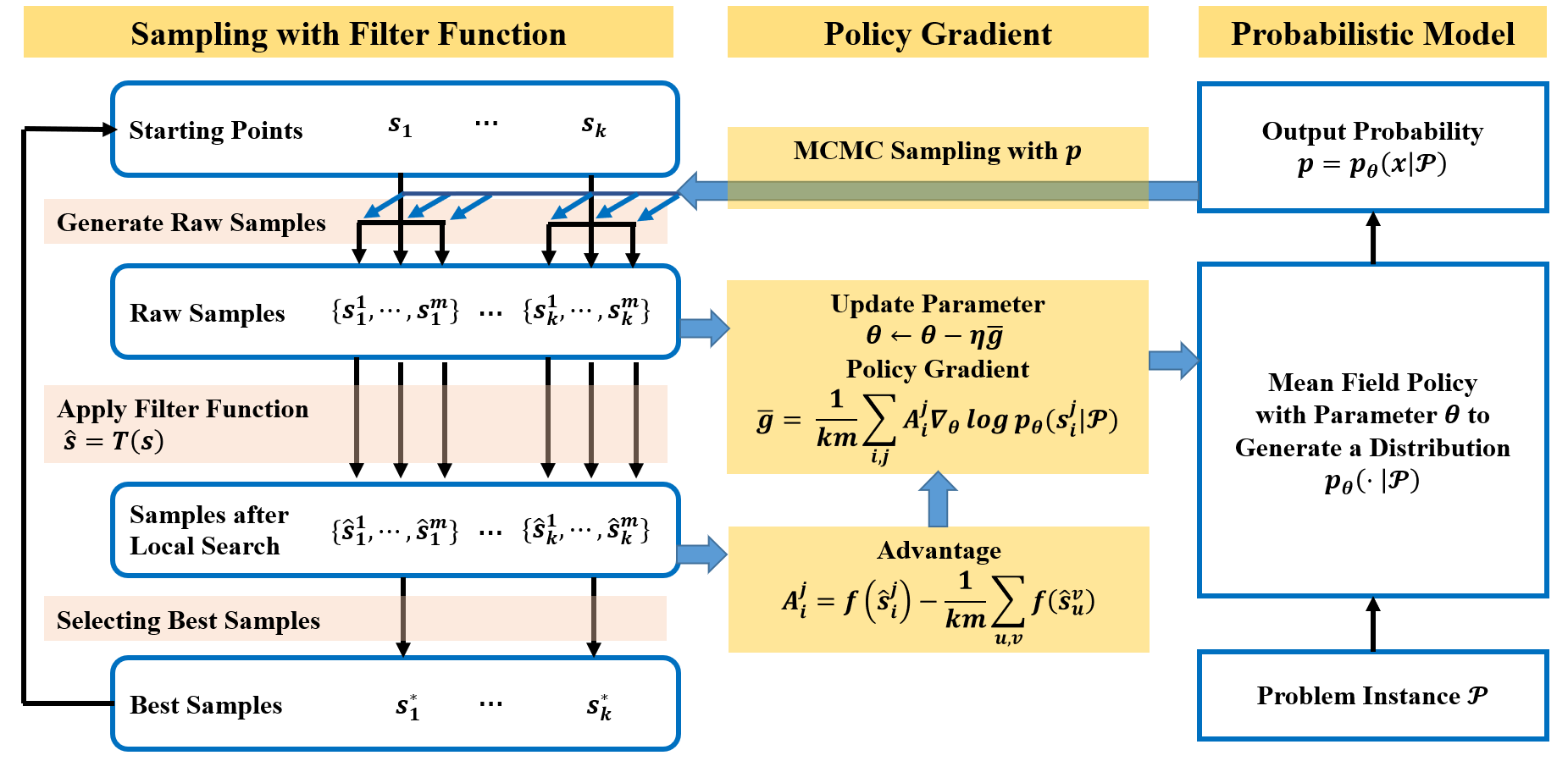
Figure 1: The pipeline of MCPG.

In the next few subsections, we first discuss the filter function. Then we present the sampling method and the update scheme in detail.

3.1 The Filter Function

The filter function $T(x)$ is a critical component of MCPG, which in essense maps an input $x$ to a better point $\hat{x}$. Since the specific details of the function $T$ depend on the structure of the problem, we next give a general definition.

Definition 1 (Filter Function)

For each $x\in\mathcal{B}_{n}$, let $\mathcal{N}(x)\subset\mathcal{B}_{n}$ be a neighborhood of $x$ such that $x\in\mathcal{N}(x)$, $|\mathcal{N}(x)|\geq 2$ and any point in $\mathcal{N}(x)$ can be reached by applying a series of “simple” operations to $x$. Then we define a filter function $T(x)$ induced by the neighborhood $\mathcal{N}(x)$ as

$$T(x)\in\mathop{\arg\min}\limits_{\hat{x}\in\mathcal{N}(x)}f(\hat{x}),$$

where $T(x)$ is arbitrarily chosen if there exists multiple solutions.

With the filter function $T$, the original binary optimization problem is converted to

$$\begin{array}[]{cc}\min&f(T(x)),\quad\text{s.t. }\quad x\in\mathcal{B}_{n}.\end{array}$$ (11)

For an optimal point $x^{*}$ of (1), it holds that $x^{*}=T(x^{*})$ and $f(x^{*})=f(T(x^{*}))$. We further have $f(T(x))\geq f(x^{*})$ because $T(x)\in\mathcal{B}_{n}$, which implies that $x^{*}$ is also the optimal point of $f(T(x))$. Therefore, the problem (11) has the same minimum value as (1). The filter function maintains the global optimal solution of $f(x)$. At the same time, it smoothens $f(x)$ and mitigates the common problem that the probabilistic model falls into a local minima during the iteration. We will demonstrate the effect of filter function at the end of this subsection.

There are many ways to choose the neighborhood $\mathcal{N}(x)$ and the filter $T$. For example, $T$ can be the projection from $x$ to the best point among its neighbors where at most $k$ variables differ from $x$, i.e.,

$$T_{k}(x)\in\mathop{\arg\min}\limits_{\|\hat{x}-x\|_{1}\leq 2k}f(\hat{x}).$$ (12)

The above procedure can be performed efficiently in parallel for all samples. Moreover, an algorithm designed to improve an input point $x$ can also serve as a filter function, even if the neighborhood set $\mathcal{N}(x)$ cannot be formulated explicitly. For example, we can introduce a greedy algorithm called Local Search (LS):

$$T_{LS}(x)=\mathtt{LocalSearch}_{f}(x).$$ (13)

LS starts with a feasible point $x^{(0)}$ and then repeatedly explores the nearby points by making small modifications to the current point. It will move to a better nearby point until a locally optimal solution is found. The pseudo-code of LS is demonstrated in Algorithm 2. Although the neighborhood $\mathcal{N}(x)$ can not be explicitly expressed in LS, it constructs a search tree during iterations. The search tree covers a wide range of points that is nearby to the input $x$.

Input: Feasible point $x$, permutation of the variable indices $I=\{i_{1},i_{2},\cdots,i_{n}\}$

1 for $t=1$ to $n$ do

2       Choose a single variable from the current point $x$ based on permutation $I$;

3       Consider the nearby set of $x$ on the index $i_{t}$

$$\mathcal{N}(x,i_{t})=\left\{x^{\prime}~{}|~{}x^{\prime}_{i_{t}}\in\{-1,1\},x^{\prime}_{j}=x_{j},\forall j\in\{1,2,\cdots,n\}\backslash\{i_{t}\}\right\};$$

4       Determine if the flipping operation is an improvement. We find the best point within $\mathcal{N}(x^{(t-1)},i_{t})$, i.e.,

$$x^{(t)}=\mathop{\arg\min}\limits_{x\in\mathcal{N}(x^{(t-1)},i_{t})}f(x);$$

5return $T_{LS}(x)=x^{(n)}$;

Algorithm 2 Local Search

We demonstrate the effect of the filter functions $T_{k}$ and $T_{LS}$ on the MaxCut problem. The MaxCut problem on the graph $G=(V,E)$ can be expressed as the following format:

$$\max\quad\sum_{(i,j)\in E}w_{ij}(1-x_{i}x_{j}),\quad\text{s.t. }\quad x\in\{-1,1\}^{n}.$$

The effect of the filter functions $T_{k}(\cdot)$ and $T_{LS}(\cdot)$ is shown in Fig. 2. The experiments are carried out on the Gset instance G22, which has 2000 nodes and 19990 edges. We first show the expectation of the objective function before and after applying the filter function. The expectation is approximated by uniform sampling. As illustrated in Section 4.1, the probabilistic model gains better performance as the expectation gets closer to the optimum. From Fig. 2(a), we find out that the expectation grows rapidly with such a simple filter function.

To illustrate the influence of the filter function, we select 20 solutions $\{x_{1},\cdots,x_{20}\}$ and depict the change of the objective function in Fig. 2(b). Each solution has only one variable differing from the preceding one, i.e., $\|x_{i+1}-x_{i}\|_{1}=2$. These points construct a “cross section” of the MaxCut problem. After applying the filter function, the function becomes smoother, leading to a reduction in the number of local maxima.

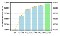
(a) The expectation of the objective function.

(b) A selected sequence of solutions.

Figure 2: The effect of the filter function for MaxCut problem on the Gset instance G22.

3.2 Parallel sampling methods with filter function

In this section we introduce our sampling method. To facilitate the application of the policy gradient, a substantial number of samples are required. Although binary solutions are relatively straightforward to obtain, direct sampling based on the Bernoulli distribution at each iteration precludes the use of previously obtained samples. Nevertheless, “old” samples are valuable in aiding the algorithmic process.

To utilize old samples, we combine the filter function with MCMC sampling techniques to enhance the quality of our samples. Algorithm 3 shows our sampling procedure for a single starting point, which is based on the Metropolis-Hastings (MH) algorithm to establish a Markov chain with the stationary distribution $p_{\theta}(\cdot)$ and is integrated with the filter function.

Input: The starting state $x_{0}$, transition number $t$, number of chain $m$, proposal distribution $Q(x^{\prime}|x)$.

1 Function sampling($x_{0}$, $t$, $m$):

2       for $j=1$ to $m$ do in parallel

3             Copy the starting state $x_{0}^{j}=x_{0}$ for this chain;

4             for $v=0$ to $t-1$ do in parallel

5                   Propose a new state $x^{\prime}$ by sampling from a proposal distribution $Q(x^{\prime}|x_{v}^{j})$;

6                   Compute the acceptance probability $\alpha(x^{\prime}|x_{v}^{j})=\min\left(1,\frac{p_{\theta}(x_{v}^{j})Q(x_{v}^{j}|x^{\prime})}{p_{\theta}(x^{\prime})Q(x^{\prime}|x_{v}^{j})}\right)$;

7                   Generate a random number $u\sim\text{Uniform}(0,1)$;

8                   if $u<\alpha(x^{\prime}|x_{v}^{j})$ then

9                        Set $x_{v+1}^{j}=x^{\prime}$;

10                        

11                  else

12                        Set $x_{v+1}^{j}=x_{v}^{j}$;

13            Obtain $s^{j}=x_{t}^{j}$;

14             Apply filter function and obtain $\hat{s}^{j}=T(s^{j})$;

15            

16      return the sample set $S=\{s^{1},s^{2},\cdots,s^{m}\}$ and $\hat{S}=\{\hat{s}^{1},\hat{s}^{2},\cdots,\hat{s}^{m}\}$;

17      

Algorithm 3 A Parallel MH algorithm with filter function

In MCPG, we choose $k$ starting points, which is selected from the best samples in the last iteration or randomly generated for the first iteration, and construct $m$ Markov chains for each of them. The computation of the $km$ chains can be carried out in parallel on the modern computational device, i.e., the outer loop is actually executed in parallel in Algorithm 3.

With the distribution $p_{\theta^{t}}(\cdot)$, the transition procedure is the same as the ordinary MH algorithm. For all the chains, we only select the last states of a chain, and obtain a sample batch $S_{i}=\{s_{i}^{1},s_{i}^{2},...,s_{i}^{m}\}$ for each of the starting point $s_{i}$. Hence, we get $k$ batches and obtain $km$ raw samples $s_{i}^{j}$ for $1\leq i\leq k,1\leq j\leq m$.

As shown in Fig. 1, the filter function is used to enhance the objective function. To fit this modification, we apply the filter function on $s_{i}^{j}$ to obtain $\hat{s}_{i}^{j}=T(s_{i}^{j})$, and these points are denoted as $\hat{S}$. This procedure can be performed efficiently in parallel for each Markov chain. Next, we compute $f(\hat{s}_{i}^{j})$ and the advantage function for the policy gradient, which will be introduced in Section 3.3.

In contrast to the standard Metropolis-Hastings algorithm, the sampling procedure in MCPG begins at multiple initial points and only retains the final states from a set of short Markov chains. The reason for this is that, parallel execution of the chains increases the diversity of the generated samples. At the same time, it saves computational time when compared to collecting states from a single but long Markov chain.

The samples in $\hat{S}$ serve an additional purpose beyond their use in the policy gradient. In practice, the samples in $\hat{S}$ are informative in identifying areas where high-quality points are likely to be found. As a result, these points are selected as initial starting points in the next iteration. To ensure the efficacy of these starting points, the maximum transition time for a single chain, represented by $t$, is set to a relatively small value. The reason is that, the samples that pass through the filter function are typically of high quality, and the adoption of a small $t$ value strikes a balance between simulating the distribution $p_{\theta}(x)$ and preserving similarity between starting points and samples.

3.3 Algorithm framework

Given a problem instance $\mathcal{P}$, our algorithmic idea is to sample the solution based on the distribution $p_{\theta^{t}}(\cdot)$ given by the probabilistic model, and use the samples to improve the probabilistic model in turn. With the filter function, MCPG focuses on the modified binary integer programming problem (11).

In fact, we can treat $f(T(\cdot))$ as a whole and denote it by $\hat{f}(\cdot)$. When replacing $f$ by $\hat{f}$, the derivation in Section 2 is still valid. Following this observation, we illustrate in detail how to update the parameters in the probabilistic model. The probabilistic model is rewritten as:

$$\min_{\theta}\quad L_{\lambda}(\theta)={\mathbb{E}_{p_{\theta}}\left[f(T(x))\right]}+\lambda{\mathbb{E}_{p_{\theta}}\left[\log p_{\theta}(x)\right]}.$$ (14)

According to the policy gradient derived in Lemma 1 in Section 2.3, we have

$$\nabla_{\theta}L_{\lambda}(\theta)=\mathbb{E}_{p_{\theta}}\left[A_{\lambda}(x;\theta)\nabla_{\theta}\log p_{\theta}(x)\right],$$ (15)

where $A(x;\theta)=f(T(x))+\lambda\log p_{\theta}(x)-\mathbb{E}_{p_{\theta}}\left[f(T(x))\right]$.

We next present a detailed description of the MCPG algorithm framework. MCPG starts from a set of randomly initialized points. For each iteration, a sample set $S=\{s_{i}^{j}|1\leq i\leq k,1\leq j\leq m\}$ is obtained from the sampling procedure introduced in Section 3.2. The filter function $T_{LS}$ is then applied to each of the solutions in the sample set $S$ to obtain $\hat{S}$. We first compute the advantage function

$$A_{\lambda}(s_{i}^{j};\theta^{t},S)=f(\hat{s}_{i}^{j})+\lambda\log p_{\theta^{t}}(s_{i}^{j})-\frac{1}{km}\sum_{u=1}^{k}\sum_{v=1}^{m}f(\hat{s}_{u}^{v}),$$ (16)

and then the policy gradient on sample set $S$ is given by

$$\bar{g}_{\lambda}(\theta^{t},S)=\frac{1}{km}\sum_{i,j}A_{\lambda}(s_{i}^{j};\theta^{t},S)\nabla_{\theta}\log p_{\theta^{t}}(s_{i}^{j}).$$ (17)

At the $t$th iteration, the parameter $\theta^{t}$ is then updated after the sampling procedure and obtaining the policy gradient by

$$\theta^{t+1}=\theta^{t}-\eta^{t}\bar{g}_{\lambda}(\theta^{t},S).$$ (18)

We can also use other stochastic gradient methods to update the parameters. Our MCPG framework is outlined in Algorithm 4. Note that the two inner loops in Algorithm 4 can be executed in parallel.

Input: number of starting points $k$, filter function $T$, number of epochs $\tau$.

1 Initialize the probabilistic model with parameters $\theta$;

2 Initialize points $s_{1},...,s_{k}$;

3 for epoch $=1$ to $\tau$ do

4       Obtain distribution $p_{\theta^{t}}(\cdot)$ from probabilistic model.;

5       for $i=1$ to $k$ do in parallel

6             $S_{i},~{}\hat{S}_{i}=\mathtt{sampling}(s_{i},t,m)$;

7            

8      Compute advantage function $A_{\lambda}(\cdot)$ on all samples in $\hat{S}_{1},\cdots,\hat{S}_{k}$ via (16);

9       Update $\theta$ using $S_{1},\cdots,S_{k}$ and $A_{\lambda}(\cdot)$ via (18) and (17);

10       Set starting point $s_{i}$ to be the best of samples in $\hat{S}_{i}$ for $i=1,\ldots,k$.;

11      

return the best solution.

Algorithm 4 MCPG

The influence of the filter function deserves to be emphasized. Maintaining sample diversity is crucial when using policy gradients. Without applying the filter function, $p_{\theta}(\cdot)$ quickly converges to local optima corresponding a few binary points, making subsequent sampling very challenging. Traditional reinforcement learning methods introduce highly technical regularization methods to avoid this problem. In contrast, the filter function in MCPG deterministically maps a large number of samples to the same local optima, thereby ensuring that $p_{\theta}(\cdot)$ does not quickly converge to a local minima. This approach guarantees diversity in subsequent sampling and facilitates continuous improvement of the model.

In the context of our well-designed sampling procedure, updating the probabilistic model involves some differences from the ordinary case. There exists bias between the distribution $p_{\theta}(\cdot)$ and the empirical distribution that are involved in the policy gradient. This bias come from the idea that the sampling procedure is designed to tend to obtain the samples of high quality, i.e., with the better objective function values, to enhance the policy gradient method. This idea is not rare in reinforcement learning. For example, assigning different priorities to samples in the replay buffer is a commonly used technique to improve performance of the policy gradient methods. In MCPG, we start the sampling procedure from the high-quality points obtained in the previous iteration to avoid worthless samples as much as possible.

3.4 Extension to problems with constraints

We now consider the constrained binary optimization problem (2) by penalizing constraint violations to force the minimum of the penalty function to lie in the feasible region of (2). The $\ell_{1}$ penalty function is introduced as

$$f_{\sigma}(x):=f(x)+\sigma\|c(x)\|_{1},$$ (19)

where $\sigma>0$ is the penalty parameter. Then, our penalty problem is:

$$x^{*}_{\sigma}=\arg\min_{x\in\mathcal{B}_{n}}f_{\sigma}(x).$$ (20)

Consequently, the unconstrained problem (20) is solved by MCPG stated in Algorithm 4. The optimal solution of (20) will be feasible to (2) if a sufficiently large penalty parameter $\sigma$ is taken. In fact, due to the limited variable space, the penalty framework (20) is exact and it has the same minimum as (20).

Proposition 1

There exists a sufficiently large value $\bar{\sigma}$ such that for all $\sigma>\bar{\sigma}$, problems (2) and (20) have the same global minimum.

Proof

Suppose that $x^{*}$ and $x^{*}_{\sigma}$ are global minimum of problems (2) and (20), respectively. Let $\varpi:=\min_{x\in\mathcal{B}_{n}}\{\|c(x)\|_{1}\mid\|c(x)\|_{1}\neq 0\}$. If there is no $x\in\mathcal{B}_{n}$ such that $\|c(x)\|_{1}\neq 0$, then all constraints $c_{i}(x)=0$ can be safely removed and (2) is reduced to the standard problem (1). Hence, we can assume that $\varpi>0$, i.e., the smallest value of $\left|{c_{i}(x)}\right|$ among all infeasible point $x$ is positive. Let $\bar{f}^{*}=\min_{x\in\mathcal{B}_{n}}f(x)$. Since $c(x^{*})=0$, we have $f(x^{*})=f_{\sigma}(x^{*})$. Hence, we can define the positive threshold value:

$$\bar{\sigma}=(f(x^{*})-\bar{f}^{*})/\varpi\geq 0.$$

We first show $x^{*}$ is a global minima of (20). For any feasible point $x$ of (2), we have

$$f_{\sigma}(x)=f(x)\geq f(x^{*})=f_{\sigma}(x^{*}).$$ (21)

On the other hand, for a point $x\in\mathcal{B}_{n}$ but $\|c(x)\|_{1}\neq 0$, it holds for $\sigma>\bar{\sigma}$ that

$$f_{\sigma}(x)=f(x)+\sigma\|c(x)\|_{1}\geq\bar{f}^{*}+\sigma\varpi>\bar{f}^{*}+(f_{\sigma}(x^{*})-\bar{f}^{*})=f_{\sigma}(x^{*}),$$ (22)

where the inequalities are due to the definitions of $\bar{f}^{*}$ and $\varpi$. Therefore, $x^{*}$ is a global optimal solution of (20).

Then, we can also prove that $x^{*}_{\sigma}$ is a global minima of (2) for any $\sigma>\bar{\sigma}$. If $\left\|{c(x^{*}_{\sigma})}\right\|_{1}\not=0$, (22) implies $f_{\sigma}(x^{*}_{\sigma})>f_{\sigma}(x^{*})$, which conflicts with the definition of $x^{*}_{\sigma}$. It shows that $x^{*}_{\sigma}$ is feasible for (2). Then for any feasible $x\in\mathcal{B}_{n}$, we have $f(x^{*}_{\sigma})=f_{\sigma}(x^{*}_{\sigma})\leq f_{\sigma}(x)=f(x)$ by the definition of $x^{*}_{\sigma}$. Therefore, $x^{*}_{\sigma}$ is a global minima of (2).

4 Theoretical analysis

Although MCPG has good practical performance, we are still concerned about its theoretical properties. In this section, we establish the relation between our proposed probabilistic solution and the optimal solution $\mathcal{X}^{*}$ in (1). It shows that minimize the expectation of $f(x)$ will increase the probability of sampling optimal solutions. Hence, the filter function is proven to improve the probabilistic model by the local search. Moreover, we illustrate the policy will be stationary and give convergence analysis of Algorithm 4 from the perspective of optimization.

4.1 Relationship between binary optimization and probabilistic model

In order to link the discrete and continuous model, we begin with the following definition to describe the properties of $f$.

Definition 2

For an arbitrary function $f$ on $\mathcal{B}_{n}$, we define the optimal gap $\mathcal{G}$ as

$$\mathcal{G}(f)=\min_{x\in\mathcal{B}_{n}\backslash\mathcal{X}^{*}}f(x)-f^{*}.$$ (23)

The bound of a function $f$ is denoted by

$$B(f)=\max_{x\in\mathcal{B}_{n}}|f(x)|.$$ (24)

A direct property of the definition is given as follows. It shows that when the probabilistic model is minimized enough, the obtained probability from the optimal solutions is linearly dependent on the gap between the expectation and the minimum of $f$.

Proposition 2

For any $0<\delta<1$, suppose $L_{\lambda}(\theta)-f^{*}<(1-\delta)\mathcal{G}(f)$, then

$$\mathbb{P}(x\in\mathcal{X}^{*})>\delta.$$

Therefore, for $x^{1},\dots,x^{m}$ independently sampled from $p_{\theta}$, $\min_{k}f(x^{k})=f^{*}$ with probability at least $1-(1-\delta)^{m}$.

Proof

Note that

$$L_{\lambda}(\theta)= \mathbb{E}_{p_{\theta}(x)}\left[f(x)\right]$$

$$= \sum_{x\in\mathcal{B}_{n}\backslash\mathcal{X}^{*}}f(x)p_{\theta}(x)+\sum_{x\in\mathcal{X}^{*}}f(x)p_{\theta}(x)$$

$$\geq \sum_{x\in\mathcal{B}_{n}\backslash\mathcal{X}^{*}}(f^{*}+\mathcal{G}(f))p_{\theta}(x)+\sum_{x\in\mathcal{X}^{*}}p_{\theta}(x)f^{*}$$

$$= f^{*}+(1-\mathbb{P}(x\in\mathcal{X}^{*}))\mathcal{G}(f).$$

Combining the above inequalities and the condition gives the conclusion.

4.2 Properties of the Filter Function

We now analyze the effect of the filter function $T$. Similar to the Gibbs distributions $q_{\lambda}(x)$ defined by (3), we also consider the Gibbs distributions $\hat{q}_{\lambda}(x)$ for filter functions as

$$\hat{q}_{\lambda}(x)=\frac{1}{\hat{Z}_{\lambda}}\exp\left(-\frac{f(T(x))}{\lambda}\right),\quad x\in\mathcal{B}_{n},$$

where $\hat{Z}_{\lambda}=\sum_{x\in\mathcal{B}_{n}}\exp\left(-\frac{f(T(x))}{\lambda}\right)$ is the normalization. In order to compare the parameterized distribution $q_{\lambda}$ and the modified distribution $\hat{q}_{\lambda}$, we utilize the KL divergence between these distributions and the parameterized distribution $p_{\theta}$. Specifically, we consider the KL divergence defined in Equation (2.1).

When $T(x)=x$, it means that $x$ is a local minimum point of $f$ in certain neighborhoods. Since $f$ is monotonically non-increasing under the filter function $T$, for any given $x\in\mathcal{B}_{n}$, there exists a corresponding local minimum point by applying the filter function $T$ to $x$ for many times. It indicates any point $x\in\mathcal{B}_{n}$ can be classified by a certain local minimum point after repetitively applying the filter function. Consequently, we can divide the set $\mathcal{B}_{n}$ into subsets with respect to the classification of local minima. Let $X_{1},X_{2},...,X_{r}$ be a partition of $\mathcal{B}_{n}$ such that for any $j\in\{1,\ldots,r\}$, every $x\in X_{j}$ has the same corresponding local minimum point. The following proposition provides a comparison between $q_{\lambda}$ and $\hat{q}_{\lambda}$.

Proposition 3

If there exists some $x\in\mathcal{B}_{n}$ such that $p_{\theta}(x)>0$ and $f(x)>f(T(x))$, then for any sufficiently small $\lambda>0$ satisfying

$$\mathbb{E}_{p_{\theta}}[f(x)-f(T(x))]\geq\lambda\log(\max_{1\leq i\leq r}|X_{i}|),$$ (25)

it holds that

$$\mathrm{KL}\left({{p_{\theta}}\,\|\,{\hat{q}_{\lambda}}}\right)\leq\mathrm{KL}\left({{p_{\theta}}\,\|\,{q_{\lambda}}}\right).$$

Proof

Let $x_{i}=\operatorname{arg~{}min}_{x^{\prime}\in X_{i}}f(x^{\prime})$ for $1\leq i\leq r$. Because of (2.1), we only need to prove that

$$\frac{1}{\lambda}\mathbb{E}_{p_{\theta}}[f(T(x))]+\log\hat{Z}_{\lambda}\leq\frac{1}{\lambda}\mathbb{E}_{p_{\theta}}[f(x)]+\log Z_{\lambda}.$$

Using (25), it suffices to prove that

$$\log\hat{Z}_{\lambda}\leq\log(\max_{1\leq i\leq r}|X_{i}|)+\log Z_{\lambda}.$$

Thus, we only need to show that

$$\sum_{x\in\mathcal{B}_{n}}\exp\left(-\frac{f(T(x))}{\lambda}\right)\leq(\max_{1\leq i\leq r}|X_{i}|)\sum_{x\in\mathcal{B}_{n}}\exp\left(-\frac{f(x)}{\lambda}\right).$$

It is true because for all $1\leq j\leq r$, we have

$$\begin{split}\sum_{x\in X_{j}}\exp\left(-\frac{f(T(x))}{\lambda}\right)&\leq|X_{j}|\exp\left(-\frac{f(x_{j})}{\lambda}\right)\\ &\leq(\max_{1\leq i\leq r}|X_{i}|)\sum_{x\in X_{j}}\exp\left(-\frac{f(x)}{\lambda}\right).\end{split}$$

This completes the proof.

The filter function $T(x)$ is induced by a given neighborhoods $\mathcal{N}(x)$ under Definition 1. Since it is hard to analyze the general case, we study a randomly chosen neighborhood and show how it improves the quality of the solutions. Note that the local search function $T_{LS}$ described in Section 3.1 is carefully designed. Therefore, it is reasonable to believe that $T_{LS}$ can also largely improve the performance of the algorithm. For convenience, we denote $N=2^{n}$ and sort all possible points in $\mathcal{B}_{n}=\{s_{1},\dots,s_{N}\}$ such that $f(s_{1})\leq f(s_{2})\leq\cdots\leq f(s_{N})$. We next show that the bounds of $f(T(x))$ and $\mathbb{E}_{p_{\theta}}[f(T(x))]$, for a large probability, are not related to samples $s_{M+1},s_{M+2},...,s_{N}$ for an integer $M$. When the neighborhood is large, then we do not need to consider most of bad samples.

Lemma 2

Suppose that the cardinality of each neighborhood $\mathcal{N}(s_{i})$ is fixed to be $|\mathcal{N}(s_{i})|\geq X\geq n+1$ and all elements in $\mathcal{N}(s_{i})$ except $s_{i}$ are chosen uniformly at random from $\mathcal{B}_{n}\backslash\{s_{i}\}$. For $\delta\in(0,1)$, let $M=\left\lceil\frac{\log(N/\delta)}{X-1}N\right\rceil+1$. Then, with probability at least $1-\delta$ over the choice of $T(x)$, it holds:

1. $f(T(x))\in[f(s_{1}),f(s_{M})],~{}\forall x\in\mathcal{B}_{n}$;

2. $\mathbb{E}_{p_{\theta}}[f(T(x))]\leq\sum_{i=1}^{M-1}p_{\theta}(s_{i})f(s_{i})+(1-\sum_{i=1}^{M-1}p_{\theta}(s_{i}))f(s_{M})\leq f(s_{M}).$

Proof

1) For all $1\leq i\leq N$, we have

$$\mathbb{P}(f(T(s_{i}))>f(s_{M}))\leq \mathbb{P}(\forall s\in\mathcal{N}(s_{i})\backslash\{s_{i}\},f(s)>f(s_{M}))$$

$$\leq \left(\frac{N-M}{N-1}\right)^{|\mathcal{N}(s_{i})|-1}\leq\left(1-\frac{M-1}{N-1}\right)^{X-1}$$

$$\leq \exp\left(-\frac{M-1}{N-1}(X-1)\right)\leq\frac{\delta}{N},$$

where the second inequality is due to $\mathbb{P}(\cup_{s}\{f(s)>f(s_{M})\})\leq\prod_{s}\mathbb{P}(f(s)>f(s_{M}))$ and $\mathbb{P}(f(s)>f(s_{M}))=(N-M)/(N-1)$ by the random choice of $s$, the third inequality uses $|\mathcal{N}(s_{i})|\geq X$, the fourth inequality uses the fact $1-x\leq e^{-x}$ and the final relies on the choice of $M$. Then, it follows that

$$\mathbb{P}(\forall x\in\mathcal{B}_{n},f(T(x))\leq f(s_{M}))\geq 1-\sum_{i=1}^{N}\mathbb{P}(f(T(s_{i}))>f(s_{M}))\geq 1-\delta.$$

2) For all $M\leq i\leq N$, we have

$$\mathbb{P}(f(T(s_{i}))>f(s_{M}))\leq\frac{\delta}{N}.$$

Hence, with probability no less than $1-\delta$ over the choice of $T$, we have

$$f(T(s_{i}))\leq f(s_{M}),\quad\forall M\leq i\leq N.$$

Therefore,

$$\mathbb{E}_{p_{\theta}}[f(T(x))]= \sum_{i=1}^{N}p_{\theta}(s_{i})f(T(s_{i}))$$

$$\leq \sum_{i=1}^{M-1}p_{\theta}(s_{i})f(s_{i})+(1-\sum_{i=1}^{M-1}p_{\theta}(s_{i}))f(s_{M}).$$

This completes the proof.

4.3 Convergence analysis of SGD

In this subsection, we will show that our algorithm converges to stationary points in expectation. It means that SGD with MCMC samples updates the policy effectively. We first make the following assumption on $p_{\theta}(x)$. For notational convenience, we write $\phi(x;\theta)=\log p_{\theta}(x)$ for any $x\in\mathcal{B}_{n}$. Without specifically mentioned, the norm used in the context will be $\ell_{2}$ norm in Euclidean space.

Assumption 1

For any $x\in\mathcal{B}_{n}$, $\phi(x;\theta)$ is differentiable with respect to $\theta$. Moreover, there exists constants $M_{1},M_{2},M_{3}>0$ such that, for any $x\in\mathcal{B}_{n}$,

1. $\sup_{\theta\in\mathbb{R}^{n}}|\phi(x;\theta)|\leq M_{1}$,

2. $\sup_{\theta\in\mathbb{R}^{n}}\left\|{\nabla_{\theta}\phi(x;\theta)}\right\|\leq M_{2}$,

3. $\left\|{\nabla_{\theta}\phi(x;\theta^{1})-\nabla_{\theta}\phi(x;\theta^{2})}\right\|\leq M_{3}\left\|{\theta^{1}-\theta^{2}}\right\|,~{}\forall\theta^{1},\theta^{2}\in\mathbb{R}^{n}$.

The above standard assumptions on the smoothness of the policy $p_{\theta}$ are adopted in several literatures on the convergence analysis of policy gradient algorithms. These can be satisfied in practice by our mean field sampling policy and neural network.

Moreover, we estimate the stochastic gradient with MCMC samples but not direct sampling. The difference is that MCMC sampling is not independent or unbiased. To explain the effectivity of MCMC, we introduce the following definitions on the finite-state time-homogenous Markov chain.

Definition 3 (spectral gap)

Let $P$ be the transition matrix of a finite-state time homogenous Markov chain. Then, the spectral gap of $P$ is defined as

$$\gamma(P):=\frac{1-\max\{|\lambda_{2}(P)|,|\lambda_{2^{n}}(P)|\}}{2}\in(0,1],$$

where $\lambda_{i}(P)$ is the $i$-th largest eigenvalue of the matrix $P$.

The spectral gap of a Markov transition matrix determines the ergodicity of the corresponding Markov chain. A positive spectral gap guarantees that the samples generated by the MCMC algorithm can approximate the desired distribution. For any non-stationary Markov chain, it will take a long time to mix until the distribution of its current state becomes sufficiently close to its stationary distribution. It leads to bias in gradient estimation. However, we can use the spectral gap to bound the bias and variance. We warm up the Markov chain and discard the beginning $m_{0}$ samples, leaving $m$ samples for estimating the stochastic gradient. The follow lemma gives error bounds of the stochastic gradient with MCMC samples.

Lemma 3

Let Assumption 1 hold and $S=\{s_{i}^{j}\}_{1\leq i\leq k,~{}1\leq j\leq m}$ be the samples generated from the MH algorithm. Suppose that the Markov chains have the stationary distribution $p_{\theta}$ and the initial distribution $\nu$. Let $\gamma=\inf_{\theta\in\mathbb{R}}\gamma(P_{\theta})\in(0,1]$ be the infimum of spectral gaps of all Markov transition matrices $P_{\theta}$. Then, the sampling error of the stochastic gradient $\bar{g}_{\lambda}(\theta,S)$ is given by

$$\left\|{\mathbb{E}_{\nu}\left[\bar{g}_{\lambda}(\theta,S)\right]-\nabla_{\theta}L_{\lambda}(\theta)}\right\| \leq\frac{\chi M_{2}(B(f\circ T)+\lambda M_{1})}{m\gamma}=:B(m),$$

$$\mathbb{E}_{\nu}\left[\left\|{\bar{g}_{\lambda}(\theta,S)-\nabla_{\theta}L_{\lambda}(\theta)}\right\|^{2}\right] \leq\frac{8nC(k)M_{2}^{2}(B(f\circ T)+\lambda M_{1})^{2}}{mk\gamma}=:V(m,k),$$

where $\chi=\chi(\nu,p_{\theta}):=\mathbb{E}_{p_{\theta}}\left[\left(\frac{d\nu}{dp_{\theta}}-1\right)^{2}\right]^{1/2}$ is the square-chi divergence between $\nu$ and $p_{\theta}$ and $C(k)=1+k\log(1+\chi)$.

Proof

We first prove that the gradient $\nabla_{\theta}L_{\lambda}(\theta)$ defined by (15) is bounded. As Assumption 1 holds, $f(T(x)),\log p_{\theta}(x),\left\|{\nabla_{\theta}\log p_{\theta}(x)}\right\|$ are bounded by $B(f\circ T),M_{1},M_{2}$ respectively. Hence, it is easily derived that $\left\|{A_{\lambda}(x;\theta)\nabla_{\theta}\log p_{\theta}(x)}\right\|$ is bounded by $(B(f\circ T)+\lambda M_{1})M_{2}$.

We now estimate the error of MCMC for an arbitrary function $h$ bounded by $M$. The empirical distribution of $s_{i}^{j}$ can be denoted by $\nu_{j}=\nu P_{\theta}^{j-1}$ for any batch $i$. Then, it follows from the Cauchy-Schwarz inequality that

$$\left|{\mathbb{E}_{\nu_{j}}[h]-\mathbb{E}_{p_{\theta}}[h]}\right|\leq\mathbb{E}_{p_{\theta}}\left[\left(\frac{d\nu_{i}}{dp_{\theta}}-1\right)^{2}\right]^{1/2}\mathbb{E}_{p_{\theta}}\left[h(x)^{2}\right]^{1/2}\leq M\chi(\nu_{j},p_{\theta}).$$ (26)

Since $\nu_{j}=\nu_{j-1}P_{\theta}$, it also holds that

$$\chi(\nu_{j},p_{\theta}) =\mathbb{E}_{p_{\theta}}\left[\left(\frac{d\nu_{j}}{dp_{\theta}}-1\right)^{2}\right]^{1/2}=\mathbb{E}_{p_{\theta}}\left[\left(\frac{d(\nu_{j-1}P_{\theta})}{dp_{\theta}}-1\right)^{2}\right]^{k/2}$$ (27)

$$\leq(1-\gamma)\chi(\nu_{j-1},p_{\theta})\leq(1-\gamma)^{j-1}\chi.$$

Hence, we denote $e_{k,m}(h)=\frac{1}{mk}\sum_{1\leq i\leq k,1\leq j\leq m}h(s^{j}_{i})$ and obtain

$$\left|{\mathbb{E}_{\nu}\left[e_{k,m}(h)\right]-\mathbb{E}_{p_{\theta}}[h]}\right| \leq\frac{1}{k}\sum_{i=1}^{k}\left|{\mathbb{E}_{\nu}\left[\frac{1}{mk}\sum_{1\leq i\leq k,1\leq j\leq m}h(s^{j}_{i})\right]-\mathbb{E}_{p_{\theta}}[h]}\right|$$

$$\leq\frac{1}{mk}\sum_{1\leq i\leq k,1\leq j\leq m}M\chi(\nu_{j},p_{\theta})$$

$$\leq\frac{1}{mk}\sum_{1\leq i\leq k,1\leq j\leq m}(1-\gamma)^{j-1}M\chi\leq\frac{M\chi}{m\gamma},$$

where the first inequality holds from (26) and the second is due to (27).

Using the following concentration inequality from Fan et al. fan2021hoeffding for the general MCMC gives

$$\mathbb{P}_{\nu}\left(e_{m,k}(h)-\mathbb{E}_{p_{\theta}}[h]>\epsilon\right)\leq(1+\chi)^{k}\exp\left(-\frac{mk\gamma\epsilon^{2}}{4M^{2}}\right).$$

Then, we can obtain the variance bound

$$\mathbb{E}_{\nu}\left[\left|{e_{k,m}(h)-\mathbb{E}_{p_{\theta}}[h]}\right|^{2}\right]= \int_{0}^{+\infty}2s\mathbb{P}_{\nu}\left(\left|{e_{m,k}(h)-\mathbb{E}_{p_{\theta}}[h]}\right|>s\right)ds$$ (28)

$$\leq \frac{8\left(1+k\log(1+\chi)\right)M^{2}}{mk\gamma}.$$

For any vector $v\in\mathbb{R}^{n}$, taking $h=v^{T}(A_{\lambda}\nabla_{\theta}\log p_{\theta})$ yields

$$\left\|{\mathbb{E}_{\nu}\left[\bar{g}_{\lambda}(\theta)\right]-\nabla_{\theta}L_{\lambda}(\theta)}\right\| =\max_{\left\|{v}\right\|=1}\left|{v^{T}\left(\mathbb{E}_{\nu}\left[\bar{g}_{\lambda}(\theta)\right]-\nabla_{\theta}L_{\lambda}(\theta)\right)}\right|$$ (29)

$$\leq\frac{\chi M_{2}(B(f\circ T)+\lambda M_{1})}{m\gamma},$$

where we use the fact that $\left|{v^{T}\nabla_{\theta}L_{\lambda}(\theta)}\right|\leq\left\|{v}\right\|\left\|{\nabla_{\theta}L_{\lambda}(\theta)}\right\|\leq(B(f\circ T)+\lambda M_{1})M_{2}$ discussed in the first paragraph of this proof. For the variance, it follows from (28) that

$$\mathbb{E}_{\nu}\left[\left\|{\bar{g}_{\lambda}(\theta,S)-\nabla_{\theta}L_{\lambda}(\theta)}\right\|^{2}\right] \leq n\max_{\left\|{v}\right\|=1}\mathbb{E}_{\nu}\left[\left|{v^{T}\bar{g}_{\lambda}(\theta,S)-v^{T}\nabla_{\theta}L_{\lambda}(\theta)}\right|^{2}\right]$$ (30)

$$\leq\frac{8n\left(1+k\log(1+\chi)\right)M_{2}^{2}(B(f\circ T)+\lambda M_{1})^{2}}{mk\gamma}.$$

This completes the proof.

The bias $B(m)$ has an order of $O\left(\frac{1}{m}\right)$ and the variance $V(m,k)$ is of $O\left(\frac{1}{mk}\right)$. The MH algorithms ensures enough locality and randomness in exploring $\mathcal{B}_{n}$. These error bounds show how hyper-parameters influence the stochastic gradient.

Under Assumption 1, we can prove the $l$-smoothness of the cost function $L_{\lambda}(\theta)$ and perform a standardized analysis in stochastic optimization. The $l$-smoothness of the loss function is shown in the following lemma.

Lemma 4

Let Assumption 1 hold. There exists a constant $l>0$ such that $L_{\lambda}(\theta)$ is $l$-smooth, that is

$$\left\|{\nabla_{\theta}L_{\lambda}(\theta^{1})-\nabla_{\theta}L_{\lambda}(\theta^{2})}\right\|\leq l\left\|{\theta^{1}-\theta^{2}}\right\|,~{}\forall\theta^{1},\theta^{2}\in\mathbb{R}^{d}.$$ (31)

Proof

For convenience, we denote that $\phi_{i}(x)=\phi(x;\theta^{i})$ and $\nabla\phi_{i}(x)=\nabla_{\theta}\phi(x;\theta^{i})$ for $i=1,2$. Under Assumption 1, it holds that for any $x\in\mathcal{B}_{n}$,

$$\left|{\phi_{i}(x)}\right|\leq M_{1}, \quad\left\|{\nabla\phi_{i}(x)}\right\|\leq M_{2},\quad\mathrm{for}~{}i=1,2,$$

$$\left|{\phi_{1}(x)-\phi_{2}(x)}\right|\leq M_{2}\left\|{\theta^{1}-\theta^{2}}\right\|, \quad\left\|{\nabla\phi_{1}(x)-\nabla\phi_{2}(x)}\right\|\leq M_{3}\left\|{\theta^{1}-\theta^{2}}\right\|.$$

Furthermore, using the Cauchy mean value theorem, we have that there exists $\lambda\in(0,1)$ such that $e^{x_{1}}-e^{x_{2}}=e^{\lambda x_{1}+(1-\lambda)x_{2}}(x_{1}-x_{2})$ for arbitrary $x_{1},x_{2}$. This fact leads to

$$\left|{e^{\phi_{1}(x)}-e^{\phi_{2}(x)}}\right| =\left|{e^{\lambda\phi_{1}(x)+(1-\lambda)\phi_{2}(x)}}\right|\left|{\phi_{1}(x)-\phi_{2}(x)}\right|$$

$$\leq\left(e^{\phi_{1}(x)}+e^{\phi_{2}(x)}\right)M_{2}\left\|{\theta^{1}-\theta^{2}}\right\|.$$

Because $p_{\theta}(x)=e^{\phi(x;\theta)}$, we can derive that

$$\nabla_{\theta}L_{\lambda}(\theta^{1})-\nabla_{\theta}L_{\lambda}(\theta^{2})$$

$$= \sum_{x\in\mathcal{B}_{n}}\left(e^{\phi_{1}(x)}(f(T(x))+\lambda\phi_{1}(x))\nabla\phi_{1}(x)-e^{\phi_{2}(x)}(f(T(x))+\lambda\phi_{2}(x))\nabla\phi_{2}(x)\right)$$

$$= \sum_{x\in\mathcal{B}_{n}}\left(e^{\phi_{1}(x)}-e^{\phi_{2}(x)}\right)(f(T(x))+\lambda\phi_{1}(x))\nabla\phi_{1}(x)$$

$$+\sum_{x\in\mathcal{B}_{n}}e^{\phi_{2}(x)}(f(T(x))+\lambda\phi_{1}(x))\left(\nabla\phi_{1}(x)-\nabla\phi_{2}(x)\right)$$

$$+\lambda\sum_{x\in\mathcal{B}_{n}}e^{\phi_{2}(x)}(\phi_{1}(x)-\phi_{2}(x))\nabla\phi_{2}(x).$$

Hence, it follows that

$$\left\|{\nabla_{\theta}L_{\lambda}(\theta^{1})-\nabla_{\theta}L_{\lambda}(\theta^{2})}\right\|$$

$$\leq \sum_{x\in\mathcal{B}_{n}}\left(e^{\phi_{1}(x)}+e^{\phi_{2}(x)}\right)M_{2}\left\|{\theta^{1}-\theta^{2}}\right\|(B(f\circ T)+\lambda M_{1})M_{2}$$

$$+\sum_{x\in\mathcal{B}_{n}}e^{\phi_{2}(x)}(B(f\circ T)+\lambda M_{1})M_{3}\left\|{\theta^{1}-\theta^{2}}\right\|+\lambda\sum_{x\in\mathcal{B}_{n}}e^{\phi_{2}(x)}M_{2}^{2}\left\|{\theta^{1}-\theta^{2}}\right\|$$

$$= \left(2M_{2}^{2}(B(f\circ T)+\lambda M_{1})+\lambda M_{2}^{2}+M_{3}(B(f\circ T)+\lambda M_{1})\right)\left\|{\theta^{1}-\theta^{2}}\right\|.$$

Let $l=2M_{2}^{2}(B(f\circ T)+\lambda M_{1})+\lambda M_{2}^{2}+M_{3}(B(f\circ T)+\lambda M_{1})$ and then (31) holds.

It follows from (31) that

$$L_{\lambda}(\theta^{2})\leq L_{\lambda}(\theta^{1})+\left\langle\nabla_{\theta}L_{\lambda}(\theta^{1}),\theta^{2}-\theta^{1}\right\rangle+\frac{l}{2}\left\|{\theta^{2}-\theta^{1}}\right\|^{2}.$$ (32)

Under our discussion, Algorithm 4 updates the policy with the stochastic gradient $\bar{g}(\theta)$. We have known the error bound of $\bar{g}(\theta)$ and $l$-smoothness of the cost function. By discussing the expected descent within each iteration, we can establish the first-order convergence and give the convergence rate as follows.

Theorem 4.1

Let Assumption 1 hold and $\{\theta^{t}\}$ be generated by MCPG. If the stepsize satisfies $\eta^{t}\leq\frac{1}{2L}$, then for any $\tau$, we have

$$\min_{1\leq t\leq\tau}\mathbb{E}\left[\left\|{\nabla_{\theta}L_{\lambda}(\theta^{t})}\right\|^{2}\right]\leq O\left(\frac{1}{\sum_{t=1}^{\tau}\eta^{t}}+\frac{\sum_{t=1}^{\tau}(\eta^{t})^{2}}{mk\sum_{t=1}^{\tau}\eta^{t}}+\frac{1}{m^{2}}\right).$$ (33)

In particular, if the stepsize is chosen as $\eta^{t}=\frac{c\sqrt{mk}}{\sqrt{t}}$ with $c\leq\frac{1}{2l}$, then we have

$$\min_{1\leq t\leq\tau}\mathbb{E}\left[\left\|{\nabla_{\theta}L_{\lambda}(\theta^{t})}\right\|^{2}\right]\leq O\left(\frac{\log\tau}{\sqrt{mk\tau}}+\frac{1}{m^{2}}\right).$$ (34)

Proof

The MCPG updates with the stochastic gradient as $\theta^{t+1}=\theta^{t}-\eta^{t}\bar{g}_{\lambda}(\theta^{t})$. For convenience, we denote that $L^{t}=L_{\lambda}(\theta^{t})$, $g^{t}=\nabla_{\theta}L_{\lambda}(\theta^{t})$ and $\hat{g}^{t}=\bar{g}_{\lambda}(\theta^{t})$ for any $t\geq 1$.Using the Lipschitz condition of $L_{\lambda}$, it follows from (32) that

$$L^{t+1} \leq L^{t}+\left\langle g^{t},\theta^{t+1}-\theta^{t}\right\rangle+\frac{l}{2}\left\|{\theta^{t+1}-\theta^{t}}\right\|^{2}$$ (35)

$$=L^{t}-\eta^{t}\left\langle g^{t},\hat{g}^{t}\right\rangle+\frac{\eta^{t2}l}{2}\left\|{\hat{g}^{t}}\right\|^{2}$$

$$=L^{t}-(\eta^{t}-\eta^{t2}l)\left\langle g^{t},\hat{g}^{t}-g^{t}\right\rangle-\left(\eta^{t}-\frac{\eta^{t2}l}{2}\right)\left\|{g^{t}}\right\|^{2}+\frac{\eta^{t2}l}{2}\left\|{\hat{g}^{t}-g^{t}}\right\|^{2}.$$

Taking the condition expectation of (35) over $\theta^{t}$, we obtain that

$$\mathbb{E}\left[L^{t+1}|\theta^{t}\right]\leq \mathbb{E}\left[L^{t}|\theta^{t}\right]-(\eta^{t}-\eta^{t2}l)\left\langle g^{t},\mathbb{E}\left[\hat{g}^{t}|\theta^{t}\right]-g^{t}\right\rangle$$ (36)

$$-\left(\eta^{t}-\frac{\eta^{t3}l}{2}\right)\left\|{g^{t}}\right\|^{2}+\frac{\eta^{t2}l}{2}\mathbb{E}\left[\left\|{\hat{g}^{t}-g^{t}}\right\|^{2}|\theta^{t}\right].$$

Using the fact $\left|{\left\langle x,y\right\rangle}\right|\leq(\left\|{x}\right\|^{2}+\left\|{y}\right\|^{2})/2$, we have

$$-(\eta^{t}-\eta^{t2}l)\left\langle g^{t},\mathbb{E}\left[\hat{g}^{t}|\theta^{t}\right]-g^{t}\right\rangle\leq\frac{\eta^{t}-\eta^{t2}l}{2}\left\|{g^{t}}\right\|^{2}+\frac{\eta^{t}}{2}\left\|{\mathbb{E}\left[\hat{g}^{t}|\theta^{t}\right]-g^{t}}\right\|^{2}.$$ (37)

Therefore, we plug in (37) to (36) and then get

$$2(\mathbb{E}\left[L^{t}|\theta^{t}\right]-\mathbb{E}\left[L^{t+1}|\theta^{t}\right])$$ (38)

$$\geq \eta^{t}\left\|{g^{t}}\right\|^{2}-\eta^{t}\cdot\left\|{\mathbb{E}\left[\hat{g}^{t}|\theta^{t}\right]-g^{t}}\right\|^{2}-\eta^{t2}l\cdot\mathbb{E}\left[\left\|{\hat{g}^{t}-g^{t}}\right\|^{2}|\theta^{t}\right]$$

$$\geq \eta^{t}\left\|{g^{t}}\right\|^{2}-\eta^{t}\cdot B^{2}(m)-\eta^{t2}l\cdot V(m,k),$$

where the second inequality is due to Lemma 3. Since $\mathbb{E}\left[L^{t}|\theta^{t}\right]=\mathbb{E}\left[L^{t}|\theta^{t-1}\right]$, summing (38) over $t=1,\dots,\tau$ and taking the total expectation yields

$$\left(\sum_{t=1}^{\tau}\eta^{t}\right)\min_{1\leq t\leq\tau}\mathbb{E}\left[\left\|{g^{t}}\right\|^{2}\right]\leq\sum_{t=1}^{\tau}\eta^{t}\cdot\mathbb{E}\left[\left\|{g^{t}}\right\|^{2}\right]$$ (39)

$$\leq 2(L^{1}-\mathbb{E}\left[L^{\tau+1}|\theta^{\tau}\right])+\sum_{t=1}^{\tau}\eta^{t2}\cdot lV(m,k)+\sum_{t=1}^{\tau}\eta^{t}\cdot B^{2}(m)$$

$$\leq O\left(1\right)+\sum_{t=1}^{\tau}\eta^{t2}\cdot O\left(\frac{1}{mk}\right)+\sum_{t=1}^{\tau}\eta^{t}\cdot O\left(\frac{1}{m^{2}}\right).$$

Dividing both sides by $\sum_{t=1}^{\tau}\eta^{t}$ gives the inequality (33).

5 Numerical results

In this section, we demonstrate the effectiveness of our algorithms on a wide variety of test problems, including MaxCut, cheeger cut, binary quadratic programming, MIMO detection problem and MaxSAT.

5.1 Experimental settings

We apply mean field approximation and express the distribution $p_{\theta}(x)$ by (8). For each variable $x_{i}$, there is a parameter $\theta_{i}$ in the probabilistic model. A sigmoid function is then applied to convert the output to the probability within $(0,1)$. In order to promote the sampling diversity, the probability is scaled to the range $(\alpha,1-\alpha)$ for a given constant $0<\alpha<0.5$. Altogether, the parameter $\mu_{i}$ in (8) is given as

$$\mu_{i}=\phi_{i}(\theta_{i})=\frac{1-2\alpha}{1+\exp(-\theta_{i})}+\alpha,\quad 1\leq i\leq n.$$ (40)

In practice, we take $\alpha=0.2$. Since a large number of samples are required in Algorithm 4, the simple scheme (8) with (40) is very fast on GPU and its performance is quite competitive to parameterization based on a few typical graph neural network in our experiments.

We compare MCPG against various methods, including state-of-the-art solvers, across all test problems. Note that MCPG utilizes the same computational device as the comparative algorithms, but additionally takes advantage of GPU acceleration. Despite MCPG described in Algorithm 4, we consider the following two variants of our algorithm:

• MCPG-U: In Algorithm 4, the sampling set $S$ is generated from the parameterized policy distribution $p_{\theta}(x)$. On the contrast, MCPG-U uses the fixed vertice-wise distribution $\mu_{i}=0.5$. Therefore, the distribution of MCPG-U is equivalent to the case when the regular factor $\lambda$ tends to infinity. The comparison between MCPG-U and Algorithm 4 illustrates the effectiveness of the parameterized policy distribution.

• MCPG-P: Existing unsupervised learning methodskaralias2020erdos use the expectation of the cost function $\mathbb{E}[f(x)]$ as the loss function to train a learning model. We notice that our sampling methods along with the filter scheme can be used as a powerful post-processing procedure. Therefore, in MCPG-P, we follow these existing learning methods to optimize the policy distribution at the beginning by minimizing $\mathbb{E}[f(x)]$, and then use this distribution instead of $p_{\theta}(x)$ to generate samples.

Our code is available at https://github.com/optsuite/MCPG.

5.2 MaxCut

The MaxCut problem aims to divide a given weighted graph $G=(V,E)$ into two parts and maximize the total weight of the edges connecting two parts. This problem can be expressed as a binary programming problem:

$$\max\quad\sum_{(i,j)\in E}w_{ij}(1-x_{i}x_{j}),\quad\text{s.t. }\quad x\in\{-1,1\}^{n}.$$ (41)

In this subsection, we show the effectiveness of our proposed algorithms on the MaxCut problems on both the Gset dataset and randomly generated graphs.

5.2.1 Numerical comparison on Gset instances

We performs experiments on standard MaxCut benchmark instances based on the publicly available Gset dataset commonly used for testing MaxCut algorithms. We select 7 graphs from Gset instances including two Erdos-Renyi graphs with uniform edge probability, two graphs where the connectivity gradually decays from node $1$ to $n$, two $4$-regular toroidal graphs, and one of the largest Gset instances.

The algorithms listed in the comparison include Breakout Local Search (BLS)benlic2013breakout , Extremal Optimization (EO)boettcher2001extremal , DSDPchoi2000solving , EMADMliu2022entropy , RUN-CSPtoenshoff2019run and PI-GNNschuetz2022combinatorial . BLS is a heuristic algorithm combining local search and adaptive perturbation, which provides most of the best known solutions for the Gset dataset. EO is a heuristic algorithm inspired by equilibrium statistical physics and is widely applied on various graph bipartitioning problems. DSDP is an SDP solver based on dual-scaling algorithm. EMADM is the another SDP-based algorithm particularly designed for binary optimization, which preserves the rank-one constraint in order to find high quality binary solutions. RUN-CSP is a recurrent GNN architecture for maximum constraint satisfaction problems. PI-GNN is an unsupervised learning methods to solve graph partitioning problems based on graph neural networks.

For BLS, DSDP, RUN-CSP and PI-GNN, we directly use the results presented in the referenced papers due to two reasons. First, the performance of all these algorithms is highly dependent on the implementation. Second, the stochastic nature of heuristic techniques inevitably leads to the deviation between the results presented in the papers and the reproduction experiments. Thus we regard the numerical experiments reported in the papers as the most reliable results.

Table 1: Computational results on selected graphs with results sourced from references.

Graph	Nodes	Edges	MCPG	BLS	DSDP	RUN-CSP	PI-GNN	EO	EMADM
G14	800	4,694	3,064	3,064	2,922	2,943	3,026	3047	3045
G15	800	4,661	3,050	3,050	2,938	2,928	2,990	3028	3034
G22	2,000	19,990	13,359	13,359	12,960	13,028	13,181	13215	13297
G49	3,000	6,000	6,000	6,000	6,000	6,000	5,918	6000	6000
G50	3,000	6,000	5,880	5,880	5,880	5,880	5,820	5878	5870
G55	5,000	12,468	10,296	10,294	9,960	10,116	10,138	10107	10208
G70	10,000	9,999	9595	9,541	9,456	-	9,421	8513	9557

Table 1 reports the best results achieved by MCPG and the comparison algorithms. It should be noticed that MCPG finds the best results for all the graphs. Compared to PI-GNN, an unsupervised learning framework, MCPG is more stable in finding the best solutions due to its efficient sampling methods and local search techniques. It is worth mentioning that the cut size $9595$ for G70 is the best-known MaxCut and is much better than previous reported results.

5.2.2 Numerical results on Gset instances within limited time

In this section, we control the running time for MCPG and report the numerical results on Gset instances. Note that some results are worse than that in Table 1, because results in Table 1 are achieved by running the algorithm with about $3-5$ times of the controlled time, and by repeating many times. We choose a heuristic-based algorithm EO and an SDP-based algorithm EMADM as the comparison algorithms. As shown in Table 1, these two algorithms achieve fairly good performance compared to other algorithms, thus we do not include other algorithms in the comparison. On the other hand, the performance of both of the two algorithms is influenced by only several hyper-parameters, and the results of the reproduction experiments are barely consistent with the results presented in the references. We describe the implementation details of the algorithms utilized in the comparison.

• EO: The standard version of EO requires $n^{2}$ iterations for the search procedure, where $n$ is the number of nodes. With this setting, the time consumption is unaffordable on large graphs, such as G81. Therefore, we set the number of iterations to $\min\{n^{2},1000n\}$ to make the time consumption comparable to MCPG.

• EMADM: The penalized SDP relaxation is solved by a first-order type method. However, the quality of the solution given by EMADM is affected by the initial point. Therefore, we report the best result of three repeated experiments as the gap of EMADM, and the time reported is the summation of the experiments.

We use the best-known results as the benchmark. Most of the best-known results are reported by BLS, except for G55 and G70, whose optimal result is found by MCPG with a long running time. Denoting $\mathrm{UB}$ as the best-known results and $\mathrm{obj}$ as the cut size, the reported gap is defined as follows:

$$\mathrm{gap}=\frac{\mathrm{UB}-\mathrm{obj}}{\mathrm{UB}}\times 100\%.$$

Table 2: Detailed result on selected Gset instances. UB is the result reported by BLS, except for G55 and G70, where we find better solutions after running MCPG for a long time.

Problem		MCPG			MCPG-U			MCPG-P			EO		EMADM
name	UB	gap		time	gap		time	gap		time	gap	time	gap	time
		(best,	mean)		(best,	mean)		(best,	mean)		mean
G22	13359	0.01	0.10	55	0.01	0.13	51	0.64	0.76	84	1.21	116	0.42	66
G23	13344	0.02	0.15	56	0.07	0.18	51	0.50	0.61	85	0.95	116	0.39	66
G24	13337	0.03	0.18	56	0.04	0.15	51	0.31	0.48	85	0.97	116	0.32	60
G25	13340	0.07	0.18	55	0.08	0.18	51	0.44	0.54	85	0.95	115	0.45	66
G26	13328	0.08	0.17	55	0.10	0.17	50	0.41	0.53	84	0.92	115	0.36	66
G27	3341	0.15	0.61	55	0.24	0.78	50	1.23	1.82	75	4.13	116	1.12	72
G28	3298	0.15	0.55	55	0.12	0.67	50	0.61	1.29	76	4.13	116	1.66	72
G29	3405	0.00	0.83	55	0.56	0.92	51	1.59	2.14	86	4.04	116	2.10	72
G30	3412	0.06	0.44	55	0.09	0.59	50	1.55	1.98	86	3.94	115	1.29	66
G31	3309	0.12	0.58	55	0.30	0.67	50	0.73	1.54	78	3.98	115	1.28	66
G32	1410	0.57	1.01	54	1.56	1.83	49	2.41	2.85	73	2.67	99	2.01	66
G33	1382	0.72	1.03	53	1.59	2.11	49	1.74	1.94	60	2.51	99	1.57	66
G34	1384	0.58	0.92	54	1.16	1.60	49	1.16	1.59	57	2.26	99	1.83	66
G35	7684	0.26	0.42	55	0.42	0.51	49	0.83	0.94	79	0.79	107	0.61	66
G36	7678	0.31	0.46	55	0.40	0.52	50	0.86	0.91	79	0.79	107	0.69	66
G37	7689	0.23	0.42	54	0.38	0.50	50	0.74	0.82	79	0.78	107	0.73	66
G38	7687	0.22	0.41	54	0.36	0.52	50	0.94	1.04	78	0.83	107	0.67	72
G39	2408	0.08	0.66	54	0.21	0.76	50	1.70	2.25	77	3.78	106	1.94	78
G40	2400	0.04	0.44	54	0.25	0.61	50	0.50	1.04	65	4.11	106	1.88	84
G41	2405	0.00	0.37	54	0.08	0.58	50	2.12	2.91	80	4.46	106	1.93	84
G42	2481	0.00	0.54	54	0.28	0.77	50	2.10	2.81	80	4.21	106	2.70	84
G43	6660	0.00	0.04	28	0.00	0.05	26	0.32	0.42	45	0.96	45	0.32	24
G44	6650	0.00	0.01	28	0.00	0.05	25	0.35	0.47	46	0.97	45	0.41	30
G45	6654	0.00	0.08	28	0.00	0.09	26	0.20	0.42	45	0.85	45	0.46	30
G46	6649	0.00	0.07	28	0.00	0.08	25	0.30	0.45	45	0.80	45	0.50	30
G47	6657	0.00	0.06	28	0.00	0.08	26	0.23	0.41	45	0.82	45	0.33	30
G55	10296	0.34	0.47	145	0.23	0.36	138	1.08	1.45	151	2.75	218	0.84	288
G56	4012	0.77	1.25	146	0.62	0.88	138	2.32	2.72	159	7.04	219	1.69	261
G57	3492	1.03	1.31	141	1.26	1.65	134	3.58	4.01	156	2.90	220	2.18	258
G58	19263	0.20	0.32	161	0.26	0.33	154	1.23	1.32	162	1.06	232	0.98	288
G59	6078	0.67	1.07	161	0.64	1.04	154	1.94	2.33	177	5.32	232	2.62	303
G60	14176	0.35	0.57	202	0.26	0.38	192	1.17	1.57	205	2.78	509	0.59	504
G61	5789	0.98	1.47	202	0.92	1.12	191	2.68	3.20	214	6.64	509	2.05	537
G62	4868	1.36	1.57	197	1.89	2.11	189	3.92	4.37	217	2.63	509	2.30	402
G63	26997	0.25	0.33	224	0.30	0.37	214	0.93	1.51	242	0.92	542	0.89	576
G64	8735	0.45	1.25	225	0.98	1.25	216	2.43	3.08	242	5.21	542	2.70	630
G65	5558	1.37	1.74	223	1.94	2.16	215	3.82	4.40	240	3.04	465	2.55	690
G66	6360	1.54	1.86	254	2.20	2.43	241	4.30	4.72	267	3.18	510	2.55	1032
G67	6940	1.38	1.57	286	1.99	2.19	270	3.79	4.53	295	2.96	550	2.51	1110
G70	9595	0.59	0.86	274	0.74	0.87	260	1.62	2.34	248	12.80	541	0.42	1194
G72	6998	1.51	1.76	284	2.17	2.40	270	4.73	5.29	294	3.09	554	2.66	1110
G77	9926	1.49	1.81	400	2.38	2.58	378	4.81	5.43	425	3.24	755	2.68	2646
G81	14030	1.74	1.98	571	2.65	2.80	559	5.26	5.57	634	3.46	1038	2.78	6144

Table 2 shows a detailed result on the medium-size graphs among Gset instances. We report the best gap (best), mean gap (mean) and mean time (time) over $20$ independent runs. Compared to the other listed algorithms, MCPG and MCPG-U achieve the maximum objective function value on all graphs except for G70. Comparing the performance of the three variants MCPG, MCPG-U and MCPG-P, we conclude that the optimized policy distribution apparently improves the performance, especially for large graphs such as G72, G77 and G81. In particular, MCPG gains a significant improvement over MCPG-U when the graph is 4-regular, such as on G32-G34.

Table 3: Detailed result on large sparse Gset instances. MCPG and its variants use edge local search as the filter function, and therefore they are suffixed by E or -E.

Problem		MCPG-E			MCPG-UE			MCPG-PE			EO		EMADM
name	UB	gap		time	gap		time	gap		time	gap	time	gap	time
		(best,	mean)		(best,	mean)		(best,	mean)		mean
G55	10296	0.11	0.34	294	0.22	0.35	288	1.08	1.45	490	2.75	218	0.84	288
G56	4012	0.67	0.88	297	0.55	0.85	289	2.32	2.72	489	7.04	219	1.69	261
G57	3492	0.86	1.09	239	0.97	1.21	229	3.58	4.01	392	2.90	220	2.18	258
G60	14176	0.24	0.38	418	0.28	0.36	398	1.17	1.57	675	2.78	509	0.59	504
G61	5789	0.71	1.00	413	0.83	0.95	396	2.68	3.20	675	6.64	509	2.05	537
G62	4868	0.99	1.26	330	1.31	1.51	323	3.92	4.37	550	2.63	509	2.30	402
G65	5558	1.19	1.46	376	1.40	1.59	369	3.82	4.40	625	3.04	465	2.55	690
G66	6360	1.29	1.47	424	1.42	1.86	416	4.30	4.72	710	3.18	510	2.55	1032
G67	6940	1.01	1.30	470	1.21	1.55	464	3.79	4.53	786	2.96	550	2.51	1110
G70	9595	0.29	0.44	480	0.24	0.42	464	1.62	2.34	398	12.80	541	0.42	1194
G72	6998	1.29	1.50	478	1.69	1.84	464	4.73	5.29	787	3.09	554	2.66	1110
G77	9926	1.35	1.52	665	1.65	1.86	649	4.81	5.43	1102	3.24	755	2.68	2646
G81	14030	1.47	1.69	946	1.94	2.06	926	5.26	5.57	1603	3.46	1038	2.78	6144

Table 3 shows a detailed result on the large sparse graphs among Gset instances by using edge local search. Edge local search is a variant of local search algorithm, which flips the two nodes of a selected edges simultaneously instead of flipping one nodes. For large sparse graphs, we find that edge local search is more efficient in finding better solutions. Though edge local search leads to more time consumption for each of the sampling procedure, the number of sampling rounds is reduced to find fairly good solutions, which maintains an acceptable time consumption. Considering the results on G77 and G81, the time consumption of EMADM increases substantially. On the contrary, to achieve a fairly good solution, MCPG and its variants cost relatively short time on large graphs, barely proportional to the the edge size, which shows the efficiency of MCPG on particularly large graphs.

5.2.3 Experiments on random regular graph

To further demonstrate the effectiveness of our proposed algorithms on large graphs, we perform the experiments on the regular graphs whose size is more than $10^{4}$ nodes. A $d$-regular graph is a graph where each vertex has $d$ neighbors. For various settings of degree $d$ and node number $n$, we randomly generate $5$ regular graphs using NetworkXSciPyProceedings_11 .

Since the optimal solutions for these randomly-generated graphs are hard to obtain, we use a relative performance measure called $P$-ratio based on the results of dembo2017extremal for $d$-regular graphs given by

$$P(z)=\frac{\mathrm{cut}/n-d/4}{\sqrt{d/4}}.$$

The $P$-ratio approaches $P^{*}\approx 0.7632$ as the number of nodes $n\to\infty$. Therefore, a $P$-ratio close to $P^{*}$ indicates that the size of the cut is close to the expected optimum.

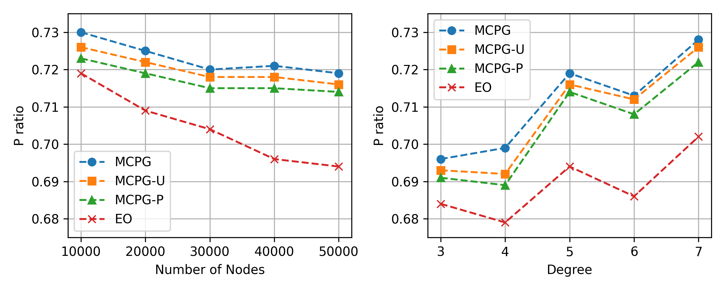
Figure 3: Computational results of regular graphs with increased number of nodes and increased number of degrees.

The tendency of the obtained cut size versus the node size and various degrees are shown in Fig. 3. We first conduct the experiment on graphs with the same degree of $5$ and an increasing number of nodes. As the number of nodes increases, the $P$-ratio for MCPG and its variants decreases slowly. Although there remains a gap between the reported $P$ value and $P^{*}$, the $P$ value obtained by MCPG is far better than the results reported in toenshoff2019run . On the contrary, as the heuristic algorithms based on local search, EO performs poorly for large graphs. It shows that the framework of MCPG is suitable for large graphs.

Table 4: Detailed computational results on random-generated regular graphs.

Problem		MCPG		MCPG-U		MCPG-P		EO
node	d	obj	p-ratio	obj	p-ratio	obj	p-ratio	obj	p-ratio
10000	5	20661	0.730	20616	0.726	20587	0.723	20537	0.719
20000	5	41206	0.725	41146	0.722	41085	0.719	40846	0.709
30000	5	61642	0.720	61584	0.718	61492	0.715	61110	0.704
40000	5	82240	0.721	82090	0.718	81958	0.715	81135	0.696
50000	3	67646	0.696	67522	0.693	67436	0.691	67129	0.684
50000	4	84932	0.699	84580	0.692	84430	0.689	83950	0.679
50000	5	102710	0.719	102529	0.716	102435	0.714	101291	0.694
50000	6	118640	0.713	118596	0.712	118326	0.708	117009	0.686
50000	7	135637	0.728	135532	0.726	135262	0.722	133920	0.702

Table 4 shows the detailed results on the randomly-generated graphs. we can see that when the degree is odd, our algorithms perform much better. The reason is that, when the degree is even, flipping the assignment of a node may lead to a tie of comparison in high probability. In all cases, MCPG outperforms all the other algorithms. For 4-regular graph with $50000$ nodes, the objective value achieved by MCPG exceeds MCPG-U over 300.

5.3 The quadratic unconstrained binary optimization (QUBO)

In this section, we demonstrate the effectiveness of our proposed algorithms on QUBO. The goal is to solve the following problem:

$$\max\quad x^{\top}Qx,\quad\text{s.t. }\quad x\in\{0,1\}^{n}.$$ (42)

Problem (42) can be reformulated as (1) by converting $\{0,1\}^{n}$ to $\{1,-1\}^{n}$ and the resulted problem still differs from the MaxCut problem due to an extra linear term. Moreover, the sparsity of $Q$ in our experiments is greater than $0.5$, which fundamentally differs from previous Gset MaxCut instances, where the sparsity is less than $0.1$.

A large and difficult datasets called NBIQ is constructed to test our algorithms. Although there are several public available datasets (such as the Biq Mac library wiegele2007biq ), most of them are generally easy for modern solvers and computing devices, and the results on them are hard to tell which algorithm is better. Therefore, we generate the NBIQ datasets, a difficult binary quadratic optimization datasets constructed by ourselves. All the instances have a density of $0.8$, which is much denser than the instances constructed from graph data. The weights are generated randomly from uniform distribution between $10$ to $100$, and they possibly turn to be negative with a given probability. By introducing the negative weights, instances of NBIQ is significantly more difficult to be solved than existing datasets. The number of variables in all these instances is more than $5000$.

We run MCPG and its variants $20$ times independently on each of the instances. Similar to the MaxCut problem, we use EMADM, an SDP solver specially designed for binary quadratic programming, as a comparison algorithm. We report the gap to the best obtained objective function value. Denoting $\mathrm{UB}$ as the best results obtained by all the listed algorithm and $\mathrm{obj}$ as the cut size, the gap reported is defined as follows:

$$\mathrm{gap}=\frac{\mathrm{UB}-\mathrm{obj}}{\mathrm{UB}}\times 100\%.$$

Table 5: Detailed result for quadratic unconstrained binary optimization.

Problem	MCPG			MCPG-U			MCPG-P			EMADM
Name	gap		time	gap		time	gap		time	gap	time
	(best,	mean)		(best,	mean)		(best,	mean)
nbiq.5000.1	0.00	0.42	364	0.24	0.45	361	0.58	0.63	364	1.33	356
nbiq.5000.2	0.00	0.50	368	0.00	0.52	364	0.93	1.08	365	1.45	361
nbiq.5000.3	0.00	0.56	370	0.29	0.68	369	0.75	0.97	378	1.23	357
nbiq.5000.4	0.00	0.69	370	0.00	0.97	367	1.82	1.88	383	1.39	362
nbiq.5000.5	0.00	0.74	374	0.17	0.89	371	1.85	1.92	376	1.41	365
nbiq.7000.1	0.00	0.39	513	0.00	0.43	510	0.54	0.60	512	1.38	1132
nbiq.7000.2	0.00	0.44	509	0.00	0.50	507	0.64	0.75	510	1.27	1147
nbiq.7000.3	0.00	0.61	515	0.34	0.90	510	1.15	1.24	512	1.47	1139
nbiq.7000.4	0.00	0.74	519	0.00	0.89	515	1.46	1.55	514	1.25	1206
nbiq.7000.5	0.00	0.92	524	0.32	1.00	522	2.26	2.40	522	1.07	1078
nbiq.10000.1	0.00	0.29	784	0.00	0.35	782	0.28	0.37	783	-	-
nbiq.10000.2	0.00	0.36	785	0.00	0.48	784	0.68	0.71	781	-	-
nbiq.10000.3	0.00	0.55	788	0.23	0.56	784	0.64	0.91	783	-	-
nbiq.10000.4	0.00	0.61	789	0.00	0.89	785	0.71	1.08	787	-	-
nbiq.10000.5	0.00	0.75	794	0.00	0.98	789	1.62	1.91	793	-	-

The results on NBIQ datasets are shown in Table 5. MCPG achieves the best objective function value in all cases. In a few cases, MCPG-U also gets the maximum objective function value obtained by MCPG. We can see that MCPG easily achieves the best known result, and it takes shorter time than EMADM on large instances. It should be noticed that the computing time of MCPG to reach the best known objective values is almost proportional to the number of nodes, which differs from EMADM and other existing algorithms.

5.4 Cheeger cut

In this subsection, we demonstrate the effectiveness of our proposed algorithms on finding the Cheeger cut. Cheeger cut is a kind of balanced graph cut, which are widely used in classification tasks and clustering. Given a graph $G=(V,E,w)$, the ratio Cheeger cut (RCC) and the normal Cheeger cut (NCC) are defined as

$$\mathrm{RCC}(S,S^{c})=\frac{\mathrm{cut}(S,S^{c})}{\min\{|S|,|S^{c}|\}},\quad\mathrm{NCC}(S,S^{c})=\frac{\mathrm{cut}(S,S^{c})}{|S|}+\frac{\mathrm{cut}(S,S^{c})}{|S^{c}|},$$

where $S$ is a subset of $V$ and $S^{c}$ is its complementary set. The task is to find the minimal ratio Cheeger cut or normal Cheeger cut, which can be converted into the following binary unconstrained programming:

$$\min \quad\frac{\sum_{(i,j)\in E}(1-x_{i}x_{j})}{\min\left\{\sum_{i}^{n}(1+x_{i}),\sum_{i}^{n}(1-x_{i})\right\}},$$

s.t. $$\quad x\in\{-1,1\}^{n},$$

and

$$\min \quad\frac{\sum_{(i,j)\in E}(1-x_{i}x_{j})}{\sum_{i}^{n}(1+x_{i})}+\frac{\sum_{(i,j)\in E}(1-x_{i}x_{j})}{\sum_{i}^{n}(1-x_{i})},$$

s.t. $$\quad x\in\{-1,1\}^{n}.$$

There are fundamental differences between the Cheeger cut problem and MaxCut problems, since the objective function of the Cheeger cut is not differentiable, which poses a challenge to algorithms based on relaxation and rounding approximations. Therefore, the framework used for many algorithms in MaxCut is not applicable to the Cheeger cut problem.

Here we conduct the experiments on the Gset instances, and compare our algorithm with p-spectral clustering (pSC) algorithm BueHei2009 . pSC regards the second eigenvector of the graph p-Laplacian as the approximation of the minimal Cheeger cut. We modify the primal pSC algorithm by adjusting the parameter $p$ during the iteration, which accelerates the algorithm by over $3$ times. We run MCPG and its variants $10$ times independently on each of the instances. We report the RCC and NCC of the partition obtained by each of the algorthms.

Table 6 presents the results obtained for finding the minimal RCC. Among all instances, MCPG consistently achieves the best objective function value. Notably, for instances G35, G36, and G37, MCPG outperforms pSC by reducing the RCC value by 0.7. Additionally, the execution time is observed to be approximately proportional to the number of graph nodes. In contrast, while pSC demonstrates moderate execution time for small graphs, it exhibits significant time growth as the graph size increases, rendering it impractical for larger instances. Specifically, the running time of pSC on large graph is more than 1.5 times longer compared to MCPG.

Table 6: Detailed result for obtaining ratio Cheeger cut (RCC).

Problem	MCPG			MCPG-U			MCPG-P			pSC
Name	RCC		time	RCC		time	RCC		time	RCC	time
	(best,	mean)		(best,	mean)		(best,	mean)
G35	2.931	3.039	66	3.036	3.163	65	3.113	3.216	65	3.864	127
G36	2.858	2.894	67	2.922	2.982	65	2.972	3.004	68	3.794	131
G37	2.847	2.899	68	2.984	3.130	69	3.050	3.173	67	3.895	134
G38	2.835	2.861	67	2.875	2.897	69	2.913	2.927	68	3.544	125
G48	0.084	0.085	93	0.085	0.088	93	0.085	0.085	94	0.109	184
G49	0.151	0.158	96	0.157	0.159	96	0.163	0.168	94	0.188	145
G50	0.033	0.034	93	0.033	0.033	95	0.034	0.035	92	0.040	140
G51	2.890	2.908	33	2.914	2.960	34	2.996	3.137	31	3.997	52
G52	2.970	2.990	35	3.083	3.149	37	3.220	3.364	33	3.993	53
G53	2.827	2.846	33	2.892	2.896	31	2.910	2.980	34	3.441	54
G54	2.852	2.918	34	2.885	3.018	32	2.928	3.016	35	3.548	57
G60	0.000	0.000	245	0.000	0.000	243	0.000	0.000	246	3.240	410
G63	3.107	3.164	242	3.233	3.358	244	3.334	3.481	241	4.090	373
G70	0.000	0.000	342	0.000	0.000	342	0.000	0.000	342	3.660	570

Table 7 displays the results obtained for finding the minimal NCC. MCPG consistently achieves the best objective function value across all instances. For instances G51-G54, MCPG achieves a reduction in NCC of $1.2$ compared to the results obtained by pSC. The analysis of consuming time for both MCPG and pSC in the context of NCC aligns with the conclusions drawn for RCC.

Table 7: Detailed result for obtaining normal Cheeger cut (NCC).

Problem	MCPG			MCPG-U			MCPG-P			pSC
Name	NCC		time	NCC		time	NCC		time	NCC	time
	(best,	mean)		(best,	mean)		(best,	mean)
G35	4.002	4.002	67	4.002	4.002	66	4.002	4.002	66	4.403	131
G36	4.002	4.002	69	4.002	4.002	70	4.002	4.002	70	5.110	136
G37	4.002	4.002	71	4.002	4.002	73	4.002	4.002	71	4.978	137
G38	4.002	4.002	68	4.002	4.002	67	4.002	4.002	68	4.448	131
G48	0.267	0.272	96	0.278	0.291	96	0.274	0.294	94	0.377	158
G49	0.088	0.091	96	0.088	0.093	96	0.091	0.097	94	0.113	174
G50	0.072	0.075	96	0.072	0.077	98	0.074	0.078	94	0.093	175
G51	4.378	4.390	34	4.523	4.606	33	4.575	4.656	35	5.689	62
G52	4.170	4.260	36	4.216	4.396	36	4.365	4.651	37	5.934	62
G53	4.171	4.193	33	4.210	4.341	33	4.215	4.500	35	5.066	60
G54	4.267	4.294	35	4.270	4.394	33	4.272	4.318	35	5.494	65
G60	0.000	0.000	255	0.000	0.000	255	0.000	0.000	255	2.150	467
G63	4.001	4.001	253	4.001	4.001	252	4.001	4.001	252	4.979	431
G70	0.000	0.000	347	0.000	0.000	345	0.000	0.000	347	4.090	636

5.5 Classical MIMO Detection

We evaluate our proposed algorithm on the classical MIMO detection problems. The goal is to recover $x_{C}\in\mathcal{Q}$ from the linear model

$$y_{C}=H_{C}x_{C}+\nu_{C},$$ (43)

where $y_{C}\in\mathbb{C}^{M}$ denotes the received signal, $H_{C}\in\mathbb{C}^{M\times N}$ is the channel, $x_{C}$ denotes the sending signal, and $\nu_{C}\in\mathbb{C}^{N}\sim\mathcal{N}(0,\sigma^{2}I_{N})$ is the Gaussian noise with known variance. We consider $\mathcal{Q}=\{z\in\mathbb{C}:{\rm Re}(z),{\rm Im}(z)\in\{\pm 1\}\}^{N}$. Our aim is to maximize the likelihood, that is equivalent to

$$\min_{x_{C}\in\mathbb{C}^{N}}\|H_{C}x_{C}-y_{C}\|_{2}^{2},\quad\text{s.t. }\quad x_{C}\in\mathcal{Q}.$$ (44)

By separating the real and imaginary parts, we can reduce the problem to a binary one. Let

$$\begin{gathered}H=\begin{bmatrix}{\rm Re}(H_{C})&-{\rm Im}(H_{C})\\ {\rm Im}(H_{C})&{\rm Re}(H_{C})\end{bmatrix},x=\begin{bmatrix}{\rm Re}(x_{C})\\ {\rm Im}(x_{C})\end{bmatrix},y=\begin{bmatrix}{\rm Re}(y_{C})\\ {\rm Im}(y_{C})\end{bmatrix}.\end{gathered}$$ (45)

The problem is equivalent to the following:

$$\min_{x\in\mathbb{R}^{2N}}\|Hx-y\|_{2}^{2},\quad\text{s.t. }\quad x\in\{\pm 1\}^{2N}.$$ (46)

Our methods are specifically designed to tackle the optimization problem represented by (46). Considering that the differences between MCPG and its variants MCPG-U and MCPG-P are minimal, particularly when the values of $M$ and $N$ are small, we have chosen to solely focus on evaluating MCPG in this context. To establish a lower bound (LB) for the problem, we assume no interference between symbols, as described in HOTML . However, it is important to note that the LB results are often unachievable in practice. For the purpose of comparison, we have evaluated our algorithm against HOTML, DeepHOTML, and minimum-mean-square-error (MMSE), as outlined in HOTML . The codes for these three algorithms were directly running on a CPU workstation.

To test the performance, we examine the bit error rate (BER) performance with respect to the signal noise ratio (SNR). The BER and SNR are defined as

$${\rm BER}=\frac{{\rm card}(\{x\neq x^{*}\})}{2N},\quad{\rm SER}=\frac{\mathbb{E}[\|H_{C}x_{C}\|_{2}^{2}]}{\mathbb{E}[\|\nu_{C}\|_{2}^{2}]}=\frac{M\sigma_{x}^{2}}{\sigma_{v}^{2}},$$ (47)

where $\sigma_{x}^{2}=\mathbb{E}[\|x_{C}\|_{2}^{2}]$, $\sigma_{\nu}^{2}=\mathbb{E}[\|\nu_{C}\|_{2}^{2}]$ are the variances, $x^{*}\in\{\pm 1\}^{2N}$ is the output solution and ${\rm card}(\{x\neq x^{*}\})$ is the cardinality of the set $\{i:x_{i}\neq x^{*}_{i}\}$. Thus, the noise becomes larger as the SNR decreases, and the problem becomes harder to solve.

To evaluate the performance of the algorithms on the problem, we conducted experiments using fixed matrix sizes $M$ and $N$, and varying signal-to-noise ratios (SNR) in the range ${2,4,6,8,10,12}$. We generated datasets consisting of either 100 or 400 randomly selected benchmarks for each fixed SNR value, and calculated the average bit error rate (BER) performance of the algorithms on these benchmarks.

Specifically, we set $M=N=180$ and $M=N=200$, and each dataset contained 400 instances. The results of these experiments are presented in Table 8 and illustrated in Fig. 4. The “Type” column in the table indicates the value of $M=N$ and the corresponding SNR(dB). It is important to note that in order to ensure appropriate termination of our algorithm, the parameters and execution times of MCPG varied depending on the SNR value. For each instance, MCPG took no more than 0.6 seconds to execute. The comparison of execution times among different algorithms was primarily focused on larger problem sizes. In terms of BER performance, MCPG consistently achieved the lowest BER among all algorithms on the datasets generated for each fixed SNR value. MCPG demonstrated improvement over the other three algorithms, particularly at SNR(dB) values of 2, 4, 6, and 8, with substantial improvement observed at SNR(dB) values of 10 and 12.

Table 8: Results on classical MIMO detection problems when $M=N=180$ and $M=N=200$.

Type	LB	MCPG		HOTML		DeepHOTML		MMSE
	BER	BER	time	BER	time	BER	time	BER	time
180-2	0.103542	0.174243	0.126	0.189819	0.238	0.176069	0.013	0.177729	0.003
180-4	0.055993	0.126701	0.149	0.143021	0.140	0.128285	0.004	0.141028	0.002
180-6	0.022729	0.070410	0.303	0.079924	0.176	0.077785	0.004	0.106201	0.002
180-8	0.006014	0.013438	0.601	0.013861	0.116	0.033701	0.005	0.075201	0.002
180-10	0.000951	0.001083	0.246	0.001313	0.081	0.007556	0.005	0.050181	0.003
180-12	0.000042	0.000042	0.246	0.000076	0.064	0.000694	0.006	0.030889	0.003
200-2	0.105538	0.174606	0.169	0.189975	0.382	0.180075	0.009	0.176825	0.003
200-4	0.057081	0.126763	0.257	0.143144	0.273	0.130656	0.006	0.140331	0.003
200-6	0.023519	0.069806	0.335	0.080588	0.294	0.076931	0.006	0.105919	0.003
200-8	0.006288	0.014556	0.581	0.015356	0.208	0.027106	0.006	0.074975	0.003
200-10	0.000856	0.001031	0.423	0.001438	0.140	0.003625	0.007	0.048950	0.004
200-12	0.000019	0.000025	0.280	0.000063	0.111	0.000100	0.006	0.030100	0.004

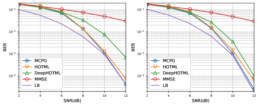
(a) $M=N=180$

(b) $M=N=200$

Figure 4: Results on classical MIMO detection problems when $M=N=180$ and $M=N=200$.

In addition to the previous experiments, we conducted further experiments on larger problem sizes, specifically $M=N=800$ and $M=N=1200$. To ensure computational efficiency, we randomly generated datasets consisting of 100 benchmarks for each case. However, due to the expensive training process of DeepHOTML, we did not run DeepHOTML for these larger cases.

The results of these experiments are presented in Table 9 and illustrated in Fig. 5. Among the three algorithms compared, MCPG consistently achieved the best performance in terms of BER on these larger cases as well. It is worth noting that at SNR(dB) values of 2, where the noise magnitude is large, it becomes challenging to improve the performance significantly. For SNR(dB) values of 4, 6, 10, and 12, MCPG demonstrates substantial improvements in performance compared to the other algorithms. Furthermore, it is important to note that while the time consumption of HOTML increases rapidly as the values of $M$ and $N$ become larger, the increment in time consumption of MCPG is not as significant. This suggests that MCPG is more computationally efficient compared to HOTML, particularly for larger problem sizes.

Table 9: Results on classical MIMO detection problems when $M=N=800$ and $M=N=1200$.

Type	LB	MCPG		HOTML		MMSE
	BER	BER	time	BER	time	BER	time
800-2	0.103731	0.174669	0.50	0.192981	10.63	0.177175	0.10
800-4	0.056331	0.126675	1.00	0.146444	11.88	0.140519	0.10
800-6	0.023131	0.069094	3.96	0.082063	13.47	0.105463	0.10
800-8	0.006300	0.012150	3.29	0.012188	6.22	0.074900	0.10
800-10	0.000969	0.001144	1.61	0.001363	3.35	0.049256	0.10
800-12	0.000031	0.000031	1.31	0.000044	2.35	0.030075	0.09
1200-2	0.104883	0.174588	1.00	0.193192	82.46	0.177675	0.45
1200-4	0.056400	0.127004	1.94	0.145813	77.83	0.140567	0.47
1200-6	0.023179	0.070346	6.47	0.083738	73.94	0.105979	0.47
1200-8	0.006179	0.012529	7.39	0.012654	61.59	0.075567	0.47
1200-10	0.000875	0.001050	5.03	0.001338	22.17	0.050167	0.46
1200-12	0.000058	0.000054	3.16	0.000071	15.70	0.030388	0.46

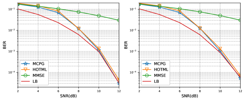
(a) $M=N=800$

(b) $M=N=1200$

Figure 5: Results on classical MIMO detection problems when $M=N=800$ and $M=N=1200$.

5.6 MaxSAT

In this subsection, we demonstrate the effectiveness of our proposed algorithms on (partial) MaxSAT problems. It is a well-known combinatorial optimization problem in computer science and operations research. Given a boolean formula in conjunctive normal form (CNF), the goal is to find an assignment of the variables that satisfies the maximum number of clauses in the formula. A formula in CNF consists of a conjunction of one or more clauses, where each clause is a disjunction of one or more literals. For example, the formula $(a\vee\neg b)\wedge(c\vee d\vee\neg e)$ is in CNF, where the first clause is $a\vee\neg b$ and the second clause is $c\vee d\vee\neg e$. Given a formula in CNF consists of clause $c^{1},c^{2},\cdots,c^{m}$, we formulate the partial MaxSAT problem as a binary programming problem as follows:

$$\max \quad\sum_{c^{i}\in C_{1}}\max\{c_{1}^{i}x_{1},c_{2}^{i}x_{2},\cdots,c_{n}^{i}x_{n},0\},$$ (48)

s.t. $$\quad\max\{c_{1}^{i}x_{1},c_{2}^{i}x_{2},\cdots,c_{n}^{i}x_{n},0\}=1,\quad\text{for }c^{i}\in C_{2},$$

$$\quad x\in\{-1,1\}^{n},$$

where $C_{1}$ represents the soft clauses that should be satisfied as much as possible and $C_{2}$ represents the hard clauses that have to be satisfied. $c_{j}^{i}$ represents the sign of literal $j$ in clause $i$, i.e.,

$$c_{j}^{i}=\begin{cases}1,&\quad\text{$x_{j}$ appears in the clause $C_{i}$},\\ -1,&\quad\text{$\neg x_{j}$ appears in the clause $C_{i}$},\\ 0,&\quad\text{else.}\\ \end{cases}$$

The constraints in the partial MaxSAT problem can be converted to an exact penalty in the objective function, which is demonstrated in (19). Since the left side of the equality constraints in (48) is no more than 1, the absolute function of the penalty can be dropped. Therefore, we have the following binary programming problem:

$$\max \quad\sum_{c^{i}\in C_{1}\cup C_{2}}w_{i}\max\{c_{1}^{i}x_{1},c_{2}^{i}x_{2},\cdots,c_{n}^{i}x_{n},0\},$$ (49)

s.t. $$\quad x\in\{-1,1\}^{n},$$

where $w_{i}=1$ for $c^{i}\in C_{1}$ and $w_{i}=|C_{1}|+1$ for $c^{i}\in C_{2}$.

We compare MCPG with its variant MCPG-U, the state-of-art incomplete solver SATLike, the state-of-art complete solver WBO and its incomplete variant WBO-inc. A complete solver tries to finds optimal solution through searching procedure and a incomplete solver usually finds a high-quality solution in the heuristic way. We do not test the learning algorithms, since they still remains poor performance compared to others. Denoting $\mathrm{UB}$ as the best results obtained by all the algorithm, and the gap reported is defined as follows:

$$\mathrm{gap}=\frac{\mathrm{UB}-\mathrm{obj}}{\mathrm{UB}}\times 100\%.$$

We first conduct the experiments on the primary MaxSAT problems without hard clauses. Since the public available datasets for primary MaxSAT is too easy for modern solvers, we randomly generate a large hard dataset. The generated clauses have at most $4$ variables. To make the problem hard and close to reality, the clauses are constructed in four ways:

• Clause with single variable $x_{i}$ or $\neg x_{i}$ is given. This type of clauses exists for all variable $x_{i}$.

• Two clauses $a_{1}\vee a_{2}$ and $\neg a_{1}\vee\neg a_{2}$ are given simultaneously, where $a_{1}$ and $a_{2}$ are randomly selected.

• Clause $a_{1}\vee a_{2}\vee a_{3}$ is given with three randomly selected variables $a_{1},a_{2},a_{3}$.

• Clauses $a_{1}\vee a_{2}\vee a_{3}\vee a_{4}$, $\neg a_{1}\vee\neg a_{2}$ and $\neg a_{3}\vee\neg a_{4}$ are given simultaneously, where the variables are randomly selected.

The results of primary MaxSAT problems are shown in Table 10. The running time of all the comparison algorithms is limited within 60, 300 or 500 seconds for instances with various sizes. MCPG outperforms all the competing algorithms, including its variant MCPG-U and the-state-of-art solvers. Not only does MCPG obtain the best results, but also the mean result of MCPG is better than the best result of other solvers. For all the three instances with 3000 variables and 10000 clauses, MCPG finds the best result every time. Note that the complete solver WBO finds the optimal solution for the two instances with 3000 variables, where MCPG also finds the optimal solution easily.

Table 10: Results on MaxSAT without hard clauses on randomly generated instances. The two columns labeled ”WBO/inc” in the table represent the respective results obtained from the WBO and WBO-inc algorithms. The computational time taken by the WBO and WBO-inc algorithms is the same as that of the SATlike algorithm.

Problem			MCPG			MCPG-U			WBO/inc		SATLike
$n$	$|C_{1}|$	UB	gap		time	gap		time	gap	gap	gap	time
			(best,	mean)		(best,	mean)
2000	8000	7211	0.00	0.00	36	0.04	0.06	36	8.17	5.74	0.08	60
2000	8000	7204	0.00	0.01	36	0.06	0.08	35	8.65	6.18	0.08	60
2000	8000	7211	0.00	0.00	36	0.01	0.06	35	8.68	6.28	0.07	60
2000	8000	7211	0.00	0.02	35	0.04	0.06	35	8.13	5.96	0.07	60
2000	8000	7200	0.00	0.00	36	0.06	0.06	35	7.89	5.78	0.07	60
2000	10000	8972	0.00	0.01	39	0.02	0.03	38	6.88	5.49	0.12	60
2000	10000	8945	0.00	0.01	39	0.02	0.05	38	6.47	5.62	0.15	60
2000	10000	8969	0.00	0.01	39	0.02	0.04	38	7.08	5.74	0.12	60
2000	10000	8950	0.00	0.01	38	0.02	0.04	38	6.74	5.89	0.13	60
2000	10000	8937	0.00	0.01	39	0.02	0.03	38	6.22	5.99	0.12	60
3000	10000	8954	0.00	0.00	160	0.02	0.05	160	0.00	5.58	0.01	300
3000	10000	8935	0.00	0.00	161	0.01	0.04	161	0.00	5.60	0.01	300
3000	10000	8926	0.00	0.00	160	0.01	0.04	161	7.78	5.39	0.01	300
3000	12000	10811	0.00	0.00	166	0.02	0.04	165	8.46	6.26	0.15	300
3000	12000	10823	0.00	0.00	166	0.01	0.03	166	8.20	5.89	0.12	300
3000	12000	10792	0.00	0.00	165	0.02	0.03	166	8.53	5.93	0.06	300
3000	15000	13712	0.00	0.00	186	0.01	0.01	185	6.66	5.49	0.13	300
3000	15000	13705	0.00	0.00	186	0.00	0.01	185	5.72	5.44	0.16	300
5000	20000	18032	0.00	0.01	341	0.05	0.06	344	7.83	6.32	0.11	500
5000	20000	18008	0.00	0.00	344	0.04	0.06	342	7.16	6.26	0.11	500

We conducted an evaluation of MCPG and other algorithms using the random track of unweighted partial MaxSAT instances from the MSE 2016 competition. The running time for all compared algorithms was limited to 60 seconds to achieve the best possible performance. For MCPG, we independently repeated the experiments 20 times on each instance and recorded the best results obtained as well as the mean gaps.

A summary of the experiments is shown in Table 11. It provides the number of the instances in which each algorithm successfully achieved the best results, i.e., the gap is zero. Notably, MCPG consistently demonstrated superior performance across various problem sets compared to SATlike. In particular, on the min2sat problem set, MCPG outperformed SATlike by obtaining the best result on 53 instances. Furthermore, MCPG achieved a mean gap of zero for 22 instances of min2sat, 33 instances of min3sat, and all other instances, indicating that MCPG achieved the best results consistently across the 20 repeated tests.

Table 11: Statistics of “gap%” on the random track datasets in MSE2016. pct denotes the ratio of num to the total number of the problem set.

Problem Set	Range	MCPG				SATlike		WBO		WBO-inc
		best		mean
		num	pct	num	pct	num	pct	num	pct	num	pct
min2sat	0.00	53	0.88	22	0.37	18	0.30	2	0.03	1	0.02
	(0.00,1.00]	7	0.12	38	0.63	31	0.52	0	0.00	8	0.13
	(1.00,2.00]	0	0.00	0	0.00	11	0.18	0	0.00	27	0.45
	(2.00,3.00]	0	0.00	0	0.00	0	0.00	0	0.00	19	0.32
	$>3.00$	0	0.00	0	0.00	0	0.00	58	0.97	5	0.08
min3sat	0.00	50	0.83	33	0.55	50	0.83	0	0.00	1	0.02
	(0.00,1.00]	5	0.08	16	0.27	3	0.05	0	0.00	2	0.03
	(0.00,2.00]	4	0.07	9	0.15	6	0.10	0	0.00	9	0.15
	(2.00,3.00]	1	0.02	1	0.02	1	0.02	0	0.00	8	0.13
	$>3.00$	0	0.00	1	0.02	0	0.00	60	1.00	40	0.67
pmax2sat	0.00	59	1.00	59	1.00	59	1.00	0	0.00	0	0.00
	(1.00,2.00]	0	0.00	0	0.00	0	0.00	0	0.00	6	0.10
	(2.00,3.00]	0	0.00	0	0.00	0	0.00	2	0.03	34	0.58
	$>3.00$	0	0.00	0	0.00	0	0.00	57	0.97	19	0.32
pmax3sat	0.00	30	1.00	30	1.00	30	1.00	0	0.00	0	0.00
	(1.00,2.00]	0	0.00	0	0.00	0	0.00	0	0.00	1	0.03
	(2.00,3.00]	0	0.00	0	0.00	0	0.00	2	0.07	13	0.43
	$>3.00$	0	0.00	0	0.00	0	0.00	28	0.93	16	0.43

The specific results for selected individual instances are provided in Table 12. It should be noted that while we controlled the running time of MCPG, other algorithms may have achieved its final results within the given time constraints. In the case of the selected min2sat results, MCPG may not have achieved the best outcome for every running time, but the average performance gap of MCPG surpasses that of SATlike. This observation highlights the superior capability of MCPG in achieving better overall results within nearly half of the runnning time compared to SATlike.

Table 12: Selected results for partial MaxSAT from the MSE 2016 competition. The two columns labeled ”WBO/inc” in the table represent the respective results obtained from the WBO and WBO-inc algorithms. Both two algorithms have the same time limits as SATlike.

Problem				MCPG			WBO/inc		SATLike
name	$|C_{2}$	$|C_{1}|$	UB	gap		time	gap	gap	gap	time
				(best,	mean)
min2sat-800-1	4013	401	340	0.00	0.00	27	24.41	2.35	1.47	60
min2sat-800-2	3983	401	352	0.00	0.06	27	24.43	0.85	0.85	60
min2sat-800-3	3956	400	340	0.00	0.03	27	22.35	1.76	0.59	60
min2sat-800-4	3933	398	349	0.00	0.00	27	26.36	2.58	1.72	60
min2sat-800-5	3871	402	353	0.00	0.42	27	20.11	1.70	0.28	60
min2sat-1040-1	4248	525	458	0.00	0.12	32	21.62	2.40	0.22	60
min2sat-1040-2	4158	528	473	0.00	0.18	33	22.83	1.27	0.21	60
min2sat-1040-3	4194	527	473	0.00	0.29	33	17.12	0.21	0.42	60
min2sat-1040-4	4079	520	474	0.00	0.14	33	18.57	1.69	0.21	60
min2sat-1040-5	4184	523	465	0.43	0.47	33	17.42	1.29	0.00	60
min3sat_v80c400_1	3931	150	95	0.00	0.84	19	23.16	6.32	1.05	60
min3sat_v80c400_2	3888	149	99	0.00	0.00	19	26.26	2.02	0.00	60
min3sat_v80c400_3	3842	141	101	0.00	0.00	19	30.69	0.00	0.00	60
min3sat_v80c400_4	3854	149	95	0.00	0.00	19	34.74	4.21	2.11	60
pmax2sat_C5000_1	150	4850	3845	0.00	0.00	19	3.17	1.85	0.00	60
pmax2sat_C5000_2	150	4850	3859	0.00	0.00	19	5.05	2.28	0.00	60
pmax2sat_C5000_3	150	4850	3851	0.00	0.00	19	4.62	1.90	0.00	60
pmax2sat_C5000_4	150	4850	3857	0.00	0.00	19	5.16	2.59	0.00	60
pmax3sat_C800_1	100	700	680	0.00	0.00	10	1.76	1.32	0.00	60
pmax3sat_C800_2	100	700	683	0.00	0.00	9	4.10	1.76	0.00	60
pmax3sat_C800_3	100	700	677	0.00	0.00	10	4.14	1.33	0.00	60
pmax3sat_C800_4	100	700	675	0.00	0.00	10	2.37	1.33	0.00	60

6 Conclusion

In this paper, we provide a new insight of the policy gradient method to solve binary optimization problems. To address the binary constraint and the discrete feasible region, we construct a probabilistic model to convert the binary optimization problems into a stochastic optimization problem. Policy gradient methods are the key to guiding the policy for searching in binary spaces. Instead of direct sampling, the MCMC sampling methods are used to preserve the locality and improve the sampling efficiency. Furthermore, we incorporate filter function, i.e., the local search algorithm, into the objective function to promote the performance. The computational results show that the proposed method can compare favorably with state-of-the-art algorithms on a variety of test problems.

There are several potential directions to be improved in the future. A better architecture of neural networks should be designed to describe the combinatorial structures. A more efficient scheme for generalization is also important. It is interesting to investigate more difficult problems, including mixed integer linear programming and nonlinear integer problems with constraints.

References

- (1) E. Aarts and J. Korst, Simulated annealing and Boltzmann machines: a stochastic approach to combinatorial optimization and neural computing, John Wiley & Sons, Inc., 1989.
- (2) Y. Bai, H. Ding, S. Bian, T. Chen, Y. Sun, and W. Wang, SimGNN: A neural network approach to fast graph similarity computation, in Proceedings of the twelfth ACM international conference on web search and data mining, 2019, pp. 384–392.
- (3) E. Baum, Towards practical neural computation for combinatorial optimization problems, in AIP Conference Proceedings 151 on Neural Networks for Computing, 1987, pp. 53–58.
- (4) U. Benlic and J.-K. Hao, Breakout Local Search for the Max-Cut Problem, Engineering Applications of Artificial Intelligence, 26 (2013), pp. 1162–1173.
- (5) S. Boettcher and A. G. Percus, Extremal optimization for graph partitioning, Physical Review E, 64 (2001), p. 026114.
- (6) C. Buchheim, M. Montenegro, and A. Wiegele, SDP-based branch-and-bound for non-convex quadratic integer optimization, Journal of Global Optimization, 73 (2019), pp. 485–514.
- (7) T. Bühler and M. Hein, Spectral Clustering based on the graph -Laplacian, in Proceedings of the 26th International Conference on Machine Learning, Omnipress, 2009, pp. 81–88.
- (8) S. Burer and R. D. Monteiro, A projected gradient algorithm for solving the maxcut SDP relaxation, Optimization methods and Software, 15 (2001), pp. 175–200.
- (9) C. Choi and Y. Ye, Solving sparse semidefinite programs using the dual scaling algorithm with an iterative solver, Manuscript, Department of Management Sciences, University of Iowa, Iowa City, IA, 52242 (2000).
- (10) A. Dembo, A. Montanari, and S. Sen, Extremal cuts of sparse random graphs, The Annals of Probability, 45 (2017), pp. 1190–1217.
- (11) R. W. Eglese, Simulated annealing: a tool for operational research, European journal of operational research, 46 (1990), pp. 271–281.
- (12) J. Fan, B. Jiang, and Q. Sun, Hoeffding’s inequality for general Markov chains and its applications to statistical learning, Journal of Machine Learning Research, 22 (2021), pp. 1–35.
- (13) P. C. Gilmore and R. E. Gomory, A linear programming approach to the cutting-stock problem, Operations research, 9 (1961), pp. 849–859.
- (14) M. X. Goemans and D. P. Williamson, . 878-approximation algorithms for MAX CUT and MAX 2SAT, in Proceedings of the twenty-sixth annual ACM symposium on Theory of computing, 1994, pp. 422–431.
- (15) G. Gutin and A. P. Punnen, The traveling salesman problem and its variations, vol. 12, Springer Science & Business Media, 2006.
- (16) A. A. Hagberg, D. A. Schult, and P. J. Swart, Exploring network structure, dynamics, and function using NetworkX, in Proceedings of the 7th Python in Science Conference, G. Varoquaux, T. Vaught, and J. Millman, eds., Pasadena, CA USA, 2008, pp. 11 – 15.
- (17) T. Hrga and J. Povh, Madam: a parallel exact solver for max-cut based on semidefinite programming and ADMM, Computational Optimization and Applications, 80 (2021), pp. 347–375.
- (18) R. Jiang, Y.-F. Liu, C. Bao, and B. Jiang, Tightness and equivalence of semidefinite relaxations for MIMO detection, arXiv preprint arXiv:2102.04586, (2021).
- (19) D. S. Johnson and L. A. McGeoch, The traveling salesman problem: A case study in local optimization, Local search in combinatorial optimization, 1 (1997), pp. 215–310.
- (20) N. Karalias and A. Loukas, Erdos goes neural: an unsupervised learning framework for combinatorial optimization on graphs, Advances in Neural Information Processing Systems, 33 (2020), pp. 6659–6672.
- (21) S. Kirkpatrick, C. D. Gelatt Jr, and M. P. Vecchi, Optimization by simulated annealing, science, 220 (1983), pp. 671–680.
- (22) N. Krislock, J. Malick, and F. Roupin, Improved semidefinite bounding procedure for solving max-cut problems to optimality, Mathematical Programming, 143 (2014), pp. 61–86.
- (23) N. Krislock, J. Malick, and F. Roupin, Biqcrunch: A semidefinite branch-and-bound method for solving binary quadratic problems, ACM Transactions on Mathematical Software (TOMS), 43 (2017), pp. 1–23.
- (24) A. Land and A. Doig, An automatic method of solving discrete programming problems, Econometrica: Journal of the Econometric Society, (1960), pp. 497–520.
- (25) H. Lemos, M. Prates, P. Avelar, and L. Lamb, Graph colouring meets deep learning: Effective graph neural network models for combinatorial problems, in 2019 IEEE 31st International Conference on Tools with Artificial Intelligence (ICTAI), IEEE, 2019, pp. 879–885.
- (26) Z. Li, Q. Chen, and V. Koltun, Combinatorial optimization with graph convolutional networks and guided tree search, Advances in neural information processing systems, 31 (2018).
- (27) H. Liu, K. Deng, H. Liu, and Z. Wen, An entropy-regularized ADMM for binary quadratic programming, Journal of Global Optimization, (2022), pp. 1–33.
- (28) O. Martin, S. W. Otto, and E. W. Felten, Large-step Markov chains for the traveling salesman problem, Citeseer, 1991.
- (29) G. Michel, X. and W. David, P., Improved approximation algorithms for maximum cut and satisfiability problems using semidefinite programming, Journal of the ACM, 42 (1995), pp. 1115–1145.
- (30) N. Mladenović and P. Hansen, Variable neighborhood search, Computers & operations research, 24 (1997), pp. 1097–1100.
- (31) A. Mobasher, M. Taherzadeh, R. Sotirov, and A. K. Khandani, A near-maximum-likelihood decoding algorithm for MIMO systems based on semi-definite programming, IEEE Transactions on Information Theory, 53 (2007), pp. 3869–3886.
- (32) R. C. Prim, Shortest connection networks and some generalizations, The Bell System Technical Journal, 36 (1957), pp. 1389–1401.
- (33) F. Rendl, G. Rinaldi, and A. Wiegele, Solving max-cut to optimality by intersecting semidefinite and polyhedral relaxations, Mathematical Programming, 121 (2010), pp. 307–335.
- (34) M. J. Schuetz, J. K. Brubaker, and H. G. Katzgraber, Combinatorial optimization with physics-inspired graph neural networks, Nature Machine Intelligence, 4 (2022), pp. 367–377.
- (35) M. Shao and W.-K. Ma, Binary MIMO detection via homotopy optimization and its deep adaptation, IEEE Transactions on Signal Processing, 69 (2021), pp. 781–796.
- (36) J. Toenshoff, M. Ritzert, H. Wolf, and M. Grohe, RUN-CSP: unsupervised learning of message passing networks for binary constraint satisfaction problems, (2019).
- (37) O. Vinyals, M. Fortunato, and N. Jaitly, Pointer networks, Advances in neural information processing systems, 28 (2015).
- (38) H.-T. Wai, W.-K. Ma, and A. M.-C. So, Cheap semidefinite relaxation MIMO detection using row-by-row block coordinate descent, in 2011 IEEE International Conference on Acoustics, Speech and Signal Processing (ICASSP), IEEE, 2011, pp. 3256–3259.
- (39) A. Wiegele, Biq Mac library—a collection of Max-Cut and quadratic 0-1 programming instances of medium size, Preprint, 51 (2007).
- (40) R. J. Williams, Simple statistical gradient-following algorithms for connectionist reinforcement learning, Machine learning, 8 (1992), pp. 229–256.
- (41) W. Yao, A. S. Bandeira, and S. Villar, Experimental performance of graph neural networks on random instances of max-cut, in Wavelets and Sparsity XVIII, vol. 11138, SPIE, 2019, pp. 242–251.