Modelling cargo transport in crowded environments: effect of motor association to cargos

Abstract

In intracellular transports, motor proteins transport macromolecules as cargos to desired locations by moving on biopolymers such as microtubules. Recent experiments suggest that cargos that can associate motor proteins during their translocation have larger run-length, association time and can overcome the motor traffic on microtubule tracks. Here, we model the dynamics of a cargo that can associate at the most $m$ free motors present on the track as obstacles to its motion. The proposed models display competing effects of association and crowding, leading to a peak in the run-length with the free motor density. This result is consistent with past experimental observations. For $m=2$ and $3$, we show that this feature is governed by the largest eigenvalue of the transition matrix describing the cargo dynamics. In all the above cases, free motors are assumed to be present as stalled obstacles. We finally compare simulation results for the run-length for general scenarios where the free motors undergo processive motion in addition to binding and unbinding to or from the microtubule.

1 Introduction

Intracellular transport often involves directional movements of motor proteins on biopolymers such as microtubules or actin filaments howard1 ; schliwa . Three major classes of motor proteins known as kinesin, dynein and myosin are responsible for such transports. Using the energy derived from the hydrolysis of adenosinetriphosphate (ATP) molecules, motor proteins transport different types of cargos such as cellular organelles, protein complexes, mRNAs etc. to desired locations in the cell. Such cargo movements are essential for various cellular functions such as cell morphogenesis, cell division, cell growth etc. This motion is processive in the sense that motor proteins typically move over several successive steps before detaching from the microtubule. Early studies block ; cross ; howard2 on intracellular transport revealed the underlying mechanism behind motor transport and how various properties such as the run-length, velocity etc. depend, for example, on the external force or the concentration of ATP molecules. While many of these studies are around the transport by a single motor, it is believed that cargos are often transported by multiple motors gross ; holzwarth ; gelfand ; unger which help cargos remain bound to the biopolymer for a longer time. Experimental and theoretical studies holzwarth ; klumpp ; beeg show that the presence of several motors helps the cargo overcome the viscous drag of the cytoplasm and have larger velocity as compared to transport by single motors. The cooperation of several motors also leads to longer run-length of the cargo before it detaches from the microtubule. Further, in vitro experiments indicate that transport processes by multiple motors can be efficiently regulated by controlling the number of engaging motors vershinin . Besides these studies, there have been extensive experimental and theoretical studies attempting to understand the collective nature of transports involving many motors under diverse conditions leduc ; segregation ; clogging ; helical ; tasep1 ; multi-opposite ; frey-lang ; multi-same ; laneswitch ; gov ; freygait .

Quite often such transport processes take place in a crowded environment of the intracellular space. This is in particular true for the axon region of the neuron cell where a dense network of biopolymers, pre-exisiting organelles and the narrow geometry of the axon together give rise to a crowded environment that can impede cargo movements. However, despite crowding, it is found that the cargo transport happens in a robust manner without significant jamming or cargo dissociation. Experiments elucidating cargo transport in crowded environments indicate that motor proteins can adapt alternative strategies that might help them circumvent the crowding problem leduc ; surrey . In a recent experimental study aimed at understanding the motion of a cargo in a crowded environment, Conway et al conway ; conway1 studied the motile properties of quantum dot (Qdot) cargos, that can associate multiple kinesins, on a microtubule crowded with free kinesin motors. While comparing the motile properties of free kinesins and the Qdot cargos in crowded conditions, cargos were found to display longer run-lengths and association times as compared to free kinesins as the motor density increased. This difference prompted the prediction that the property of a cargo to associate multiple motors helps increase its run-length, association time and overcome the motor traffic. It was observed that while translocating, Qdot cargos could associate kinesins from the microtubule pool, dissociate kinesins attached to itself, or associate kinesins that are already moving along the microtubule and move together subsequently.

Motivated by this work, here, we propose mathematical and computational models to characterise the motion of a single cargo on a track crowded by free kinesin motors. During its translocation, the cargo can associate free motors which impede the motion of the cargo by occupying the forward sites on the microtubule. We assume that upon such association, a kinesin detaches itself from the microtubule rendering the forward site free. Our aim is to find how the interplay of the kinesin-association property of the cargo and the crowding along the track affects cargo’s motile properties, for example, its run-length and association time etc. To our knowledge, this is the first modelling study of cargo transport where the cargo has the ability to associate kinesins present on a crowded microtubule track.

To this end, we study cargo transport under different scenarios described below. (1) In the simplest scenario, we assume that the cargo is always bound to the microtubule. Along the path of the cargo, the microtubule binding sites are randomly occupied by free kinesin motors. We assume that the kinesin that gets associated to the cargo during its translocation plays no specific role in facilitating the forward motion of the cargo other than freeing the forward site. This is equivalent to assuming that the cargo removes the kinesin molecule occupying the forward site via the association process. For this model, referred as "Model 1" below, we find the average velocity of the cargo. (2) In model 2, we assume that the cargo can bind more than one, say, at the most $m$ number of kinesins. This is based on the predictions that the cargo may have a finite number of kinesin binding sites conway . Hence, the cargo can associate a kinesin occupying the forward site provided it has a free binding site available. We consider $m=2,\ 3,{\rm and}\ 4$ in the following analysis. Kinesins attached to the cargo can detach from it and a free kinesin from the intracellular space can attach to the cargo at given rates. Finally, we implement the condition that a cargo can no longer be on the microtubule track if all the kinesin molecules detach from the cargo. A generalised version of the mathematical formulation of model 1 allows us to analyse the cargo motion obeying above rules for $m=2$ and $3$. Finally, run-lengths of $m=2,\ 3,{\rm and\ 4}$ are found upon numerically simulating the cargo dynamics. The motion of the cargo following different dynamical rules are shown in figure 1.

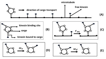
Figure 1: (A) Cargo transport on a microtubule in the presence of free kinesins bound to microtubules. The microtubule is represented by a one-dimensional lattice with a site representing a tubulin dimer, the basic subunit of a microtubule. (B) A cartoon of a cargo bound to two kinesins. The cargo has more than one kinesin binding sites. (C) The process of kinesin association to cargo at rate $r_{an}$. (D) The process of attachment of a kinesin from the intracellular space to the cargo at rate $\omega_{a}$. (E) The process of kinesin detachment from the cargo at rate $\omega_{d}$.

(3) In models 1 and 2, free kinesins are assumed to be stalled on the microtubule. In model 3, we simulate cargo dynamics in the presence of moving kinesins as well as random processes of kinesin binding and unbinding to or from the microtubule. We compare the run-length of the cargo (with $m=3$) in the presence or absence of various processes mentioned above.

2 Models and Results

2.1 Model 1

The motion of the cargo is modelled considering the following dynamical rules. (a) The cargo transported by a kinesin starts its forward journey from a given point on a one-dimensional track (often referred below as a lattice) representing the microtubule. (b) For all the lattice sites ahead, we assume an initial, random distribution of free kinesins. The average kinesin density on the lattice is represented by $r_{m}$. These kinesins are assumed to be stalled. (c) The cargo moves to the forward site provided the forward site is not occupied by a free kinesin. (d) If the forward site in front of the cargo is occupied by a free kinesin, the cargo can associate the kinesin with itself at rate $r_{an}$ rendering the forward site free.

In order to build the mathematical model, we consider possible configurations that two neighbouring sites can have when the first one of them is occupied by the cargo. For $i$ and $(i+1)$-th sites, with the cargo being at the $i$-th site, the $(i+1)$-th site can be either empty or occupied by a free kinesin molecule. We denote the probability of finding $(i+1)$-th site empty with the $i$-th site occupied by the cargo at time $t$ by $P(i,t)$. Similarly, the probability of finding $(i+1)$-th site occupied by a free kinesin while the cargo is at the $i$-th site at time $t$ is $Q(i,t)$. Figure (2) shows these configurations as well as possible transitions from one configuration to the other as the cargo translocates forward. The following equations describe how these two configurations evolve with time sm .

$$\frac{dP(i)}{dt}=r_{an}Q(i)+(1-r_{m})P(i-1)-P(i),$$

(1)

$$\frac{dQ(i)}{dt}=-r_{an}Q(i)+r_{m}P(i-1).$$ (2)

The first term on the RHS of equation (1) indicates a cargo-association process due to which a Q-type configuration transitions to a $P$-type configuration. The term with the pre-factor $(1-r_{m})$ indicates the motion of the cargo from $(i-1)$-th site to $i$-th site while the $(i+1)$-th site is vacant. While the forward motion happens with unit rate, the factor $(1-r_{m})$ indicates the probability that after the forward motion, $(i-1)\rightarrow i$, the cargo lands in a P-type configuration i.e. the $(i+1)$-th site is unoccupied by a kinesin. The last term in (1) is a loss term which indicates that a cargo has moved from the $i$-th site to the $(i+1)$-th site. In equation (2), the first term on the RHS indicates a loss of a $Q$-type configuration due to the association process. The second term is a gain term due to the hopping of the cargo from $(i-1)\rightarrow i$ where $(i+1)$-th site is occupied by a free kinesin.

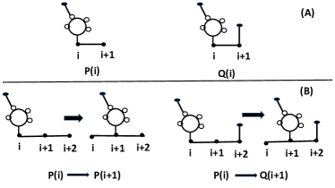
Figure 2: (A) Two possible configurations of two neighbouring sites with the first site occupied by the motor transporting the cargo. (B) Possible transitions associated with the transport of the cargo to the next site.

To find the average properties of the cargo motion, we define generating functions corresponding to the two probabilities as

$$\tilde{P}(\gamma)=\sum_{i=-\infty}^{\infty}\gamma^{i}P(i),\ {\rm and}\ \tilde{Q}(\gamma)=\sum_{i=-\infty}^{\infty}\gamma^{i}Q(i).$$ (3)

In terms of these generating functions, the time evolution equations are

$$\frac{d}{dt}\tilde{P}(\gamma)=r_{an}\tilde{Q}(\gamma)+(1-r_{m})\gamma\tilde{P}(\gamma)-\tilde{P}(\gamma),\ {\rm and}$$

(4)

$$\frac{d}{dt}\tilde{Q}(\gamma)=-r_{an}\tilde{Q}(\gamma)+r_{m}\gamma\tilde{P}(\gamma).$$ (5)

The average position of the cargo can be found from the probabilities as

$$\langle i\rangle=\sum_{i=-\infty}^{\infty}i[P(i)+Q(i)]=\frac{d}{d\gamma}[\tilde{P}(\gamma)+\tilde{Q}(\gamma)]\mid_{\gamma=1}.$$ (6)

The average velocity of the cargo is obtained from $v=\langle i\rangle/t$ where $t$ is the time taken to travel an average distance $\langle i\rangle$. Solving equations (4) and (5), the average velocity of the cargo is found as (see Appendix A for details)

$$v=\frac{r_{an}}{r_{an}+r_{m}}.$$ (7)

2.2 Model 2

Here we generalize the mathematical framework, discussed in the previous section, for higher values of $m$ taking into account the possibilities of detachments of the cargo from the microtubule. In the following, we discuss the mathematical model for $m=2$ and simulation results for $m=2,\ 3,\ {\rm and}\ 4$. The cargo dynamics for $m=3$ is discussed in Appendix B.

For $m=2$, the cargo has two kinesin binding sites. Hence it can associate at the most two kinesins. The basic rules for cargo transport in this case are listed below. (a) As before, we begin with an initial, random distribution of stalled free kinesins on a one-dimensional lattice. The average density of free kinesins is $r_{m}$. (b) The cargo attached to a kinesin starts its forward journey from a given point on the lattice. (c) If the forward site is blocked by a free kinesin, the cargo can associate the kinesin with itself at a rate $r_{an}$ provided the cargo has only one kinesin bound to it. (d) A kinesin bound to the cargo can detach from the cargo at rate $\omega_{d}$ and a free kinesin from the intracellular space can bind to the cargo at rate $\omega_{a}$ provided the cargo has only one kinesin attached to it. (e) A cargo is not attached to the microtubule if all the kinesins detach from the cargo. Thus, we are not being specific about how many kinesins are actively transporting the cargo or how many remain bound to the cargo without participating in cargo transport actively.

As before, we begin with two possible configurations of, say, $\{i,i+1\}$-th sites where $i$-th site is occupied by the cargo. However, here the cargo can be in two possible states - bound to one kinesin or bound to two kinesins. Hence, the probabilities are defined in the following way. $P_{n}(i,t)$ ($n=1,\ 2)$ represents the probability, at time $t$, of the configuration where the cargo, located at $i$-th site, is bound to $n$ kinesins and the $(i+1)$-th site is empty. Similarly, $Q_{n}(i,t)$ ($n=1,\ 2$) represents the probability, at time $t$, of the configuration where the cargo, located at $i$-th site, is bound to $n$ kinesins and the $(i+1)$-th site is occupied by a free kinesin.

The probabilities of various configurations change with time as per the following equations,

$$\frac{d}{dt}P_{2}(i)=(1-r_{m})P_{2}(i-1)-P_{2}(i)+r_{an}Q_{1}(i)-\omega_{d}P_{2}(i)+\omega_{a}P_{1}(i),$$ (8)

$$\frac{d}{dt}P_{1}(i)=(1-r_{m})P_{1}(i-1)-P_{1}(i)-\omega_{a}P_{1}(i)+\omega_{d}(P_{2}(i)-P_{1}(i)),$$ (9)

$$\frac{d}{dt}Q_{2}(i)=r_{m}P_{2}(i-1)+\omega_{a}Q_{1}(i)-\omega_{d}Q_{2}(i),\ {\rm and}$$ (10)

$$\frac{d}{dt}Q_{1}(i)=r_{m}P_{1}(i-1)-r_{an}Q_{1}(i)+\omega_{d}(Q_{2}(i)-Q_{1}(i))-\omega_{a}Q_{1}(i).$$ (11)

The $r_{\rm an}$-dependent term in equation (8) represents a process of kinesin association by the cargo. Due to this process, a $Q_{1}$-type configuration transitions to a $P_{2}$-type configuration. $\omega_{a}$($\omega_{d}$) dependent terms represent kinesin attachment(detachment) processes to(from) the cargo. For example, the $\omega_{d}$ dependent term in equation (8) represents detachment of a kinesin due to which the cargo transitions from $P_{2}$ state to $P_{1}$ state. In addition to above equations, we introduce probabilities $P_{0}(i,t)$ and $Q_{0}(i,t)$ of having situations where the cargo bound to one kinesin residing at $i$-th site at time $t$ loses its kinesin. These probabilities change with time as per the equations

$$\frac{d}{dt}P_{0}(i)=\omega_{d}P_{1}(i)\ {\rm and}\ \frac{d}{dt}Q_{0}(i)=\omega_{d}Q_{1}(i).$$ (12)

Defining generating functions as $\tilde{P}_{n}(\gamma,t)=\sum_{i=-\infty}^{\infty}\gamma^{i}P_{n}(i,t)$, and $\tilde{Q}_{n}(\gamma,t)=\sum_{i=-\infty}^{\infty}\gamma^{i}Q_{n}(i,t)$ (where $n=0,\ 1,\ 2$), we can rewrite equations (8)-(11) as

$$\frac{d}{dt}{\bf H}(\gamma,t)={\bf S}{\bf H}(\gamma,t),$$ (13)

where ${\bf H}$ is a column matrix

$${\bf H}(\gamma,t)={\begin{pmatrix}&\tilde{P}_{2}(\gamma,t)\\ &\tilde{P}_{1}(\gamma,t)\\ &\tilde{Q}_{2}(\gamma,t)\\ &\tilde{Q}_{1}(\gamma,t)\\ \end{pmatrix}}$$ (14)

and ${\bf S}$ is a $4\times 4$ matrix

$${\bf S}={\begin{pmatrix}&(1-r_{m})\gamma-1-\omega_{d}&\omega_{a}\ &0&r_{an}\\ &\omega_{d}&(1-r_{m})\gamma-1-\omega_{a}-\omega_{d}&0&0\\ &r_{m}\gamma&0&-\omega_{d}&\omega_{a}\\ &0&r_{m}\gamma&\omega_{d}&-(\omega_{a}+\omega_{d}+r_{an})\\ \end{pmatrix}}.$$ (15)

In order to have an estimate of the association time of the cargo and how it is impacted by various processes, we have studied the quantity $[\tilde{P}_{0}(\gamma,t)+\tilde{Q}_{0}(\gamma,t)]\mid_{\gamma=1}$. This quantity being identical to $\sum_{i=-\infty}^{\infty}[P_{0}(i,t)+Q_{0}(i,t)]$ indicates the total probability of cargo being left with no kinesin bound to it while being at any point on the lattice. A plot of this quantity for different parameter values are shown in figures (3) and (4). Over large time, this quantity approaches unity indicating cargo losing all the kinesins leading to the detachment of the cargo from the microtubule. The approach of this quantity to unity is what provides us with an estimate of the association time of the cargo to the microtubule. A fast approach to unity indicates a low association time of the cargo. For both figures, we have chosen the same sets of values for the kinesin-association rate, $r_{an}$. The increase or decrease in $\omega_{a}$ and $\omega_{d}$, respectively, is expected to increase the association time of the cargo. Figures show that reducing the kinesin detachment rate, $\omega_{d}$, from the cargo has much stronger effects on the association time as compared to increasing the kinesin attachment rate, $\omega_{a}$.

Figure 3: $y-$axis represents the total probability ($\sum_{i=-\infty}^{\infty}[P_{0}(i,t)+Q_{0}(i,t)]$) of the cargo losing its last kinesin at time $t$ while being at any site on the lattice. For this plot, $r_{m}=0.5$ and $\omega_{a}=0.01$.

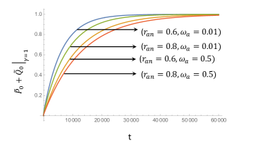
Figure 4: $y-$axis represents the total probability ($\sum_{i=-\infty}^{\infty}[P_{0}(i,t)+Q_{0}(i,t)]$) of the cargo losing its last kinesin at time $t$ while being at any site on the lattice. For this plot, $r_{m}=0.5$ and $\omega_{d}=0.01$.

In figure (5), we have shown how the total probability of cargo detachment at any point on the lattice is influenced by the kinesin density, $r_{m}$. The figure shows that at a low value of the kinesin-association rate by the cargo, $r_{\rm an}$, the extent of crowding influences the cargo-association time to the microtubule only mildly. The situation changes significantly when the kinesin-association rate is high. In this case, the association time of the cargo to the microtubule, in general, increases significantly. Further, for large $r_{\rm an}$, the crowding density of free kinesins affects the association time of the cargo significantly with the association time being larger for lower crowding density.

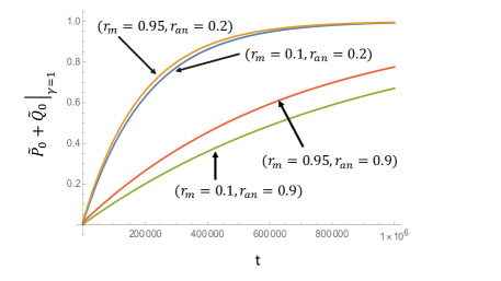
Figure 5: $y-$axis represents the total probability ($\sum_{i=-\infty}^{\infty}[P_{0}(i,t)+Q_{0}(i,t)]$) of the cargo losing its last kinesin at time $t$ while being at any site on the lattice. For this plot, $\omega_{a}=\omega_{d}=0.001$.

The dependence of the run-length of the cargo on the crowding density can be obtained upon solving equations (8)-(11) numerically. Figure (6) shows run-length plots for different values of the kinesin-association rate, $r_{\rm an}$, and kinesin attachment and detachment rates, $\omega_{a}$ and $\omega_{d}$, respectively. For small $r_{\rm an}$, the run-length decreases monotonically. However, for large $r_{\rm an}$, the run-length increases initially for low crowding. In this case, due to large $r_{\rm an}$, the cargo benefits from the kinesin-association process at low crowding. As the crowding density increases, due to limited number of binding sites, the cargo no longer benefits from kinesin association and the run-length decreases. This variation of the run-length with the crowding density is consistent with earlier experimental predictions conway . With the increase in the kinesin detachment rate, $\omega_{d}$, the run-length of the cargo decreases significantly. However, as found earlier, a decrease in the rate of kinesin attachment, $\omega_{a}$, to the cargo has mild effect on cargo’s run-length.

Figure 6: Run-length of the cargo plotted with crowding density, $r_{m}$. The cargo can bind at the most two kinesins ($m=2$).

The fact that the run-length of the cargo for high kinesin-association rates increases with the crowding density initially is consistent with the estimates obtained from the analysis of the largest eigenvalue of the transition matrix $S$ and the association time. In the limit of large time, the solutions for the probabilities are given by

$${\bf H}\approx c_{1}e^{\lambda_{l}t}{\bf X},$$ (16)

where $c_{1}$ is a constant, $\lambda_{l}$ is the largest of the four eigenvalues of the transition matrix ${\bf S}$ with all of them being negative and ${\bf X}=(x_{1},\ x_{2},\ x_{3},\ x_{4})^{T}$ is the corresponding eigenvector. The average distance travelled by the cargo and its average velocity can be obtained from $\langle i\rangle=\sum_{i=-\infty}^{\infty}i[P_{1}(i,t)+P_{2}(i,t)+Q_{1}(i,t)+Q_{2}(i,t)]\\ =\gamma\frac{d}{d\gamma}[\tilde{P}_{1}(\gamma,t)+\tilde{P}_{2}(\gamma,t)+\tilde{Q}_{1}(\gamma,t)+\tilde{Q}_{2}(\gamma,t)]\mid_{\gamma=1}$ and $v={\langle i\rangle}/{t}$, respectively. In the large time limit, the dominant contribution to the velocity is of the form $v\approx[\gamma c_{1}e^{\lambda_{l}t}\frac{d\lambda_{l}}{d\gamma}\sum_{i=1}^{4}x_{i}]\mid_{\gamma=1}$. Using $1/\lambda_{l}$ as an estimate of the association time, $t_{\rm assoc}$, and finding $\frac{d\lambda_{l}}{d\gamma}\mid_{\gamma=1}$ numerically for given parameter values, we have plotted $t_{\rm assoc}\frac{d\lambda_{l}}{d\gamma}\mid_{\gamma=1}$ as a function of the crowding density, $r_{m}$, in figure (7). Plots in figure (7) display similar trends as found in figure (6) for the run-length. Although $t_{\rm assoc}v$ gives an estimate of the run-length, the variation in the run-length with the crowding density as seen in figure (6) essentially arises from $t_{\rm assoc}\frac{d\lambda_{l}}{d\gamma}\mid_{\gamma=1}$. It can be verified numerically that the variation in the remaining factors in $v$ is almost negligible over the entire range of $r_{m}$, $[0:1]$.

Figure 7: $y$-axis represents the product of two factors that dominate the nature of the run-length. $t_{\rm assoc}$ is the association time of the cargo and $\frac{d\lambda_{l}}{d\gamma}$ arises while computing the average velocity of the cargo (see the text). This plot is for $m=2$ with $\omega_{a}=\omega_{d}=0.001$.

The dynamical equations for a cargo that can bind at the most three kinesins, i.e. $m=3$, are shown in Appendix B. The variation of $t_{\rm assoc}\frac{d\lambda_{l}}{d\gamma}\mid_{\gamma=1}$ with the crowding density as obtained from the analysis of the largest eigenvalue is shown in figure (14).

Next we simulate the cargo dynamics with the cargo having $m=2,\ 3,{\rm and}\ 4$ kinesin binding sites. Figure (8) shows the change in the run-length of the cargo with free-kinesin density, $r_{m}$, for $m=2,\ 3,\ {\rm and}\ 4$. Simulations show an initial increase in the run-length with the free-kinesin-density for $m=3\ {\rm and}\ 4$; a trend that was shown earlier in figure (6).

Figure 8: Run-length of the cargo as a function of free-kinesin density along the microtubule track. For this figure, $\omega_{a}=\omega_{d}=0.05$, $r_{an}=0.4$. The results are obtained upon averaging over $500$ samples for $m=2$ and $3$, and over $1500$ samples for $m=4$.

2.3 Processive motion of free kinesins for $m=3$

In this section, we study the motion of the cargo in the presence of free kinesins which move processively on the microtubule track. In addition, kinesins from the intracellular environment can attach to the microtubule and those walking on the microtubule can leave the microtubule at given rates.

Here we simulate this system using the cellular automaton method. As before, the microtubule is represented by a one-dimensional lattice. We begin with the cargo positioned at one end of the lattice. The lattice sites are randomly occupied by free kinesins with an average density, $r_{m}$. The cargo moves following the association mechanism mentioned earlier. We assume that the kinesins move unidirectionally in the same direction as that of the cargo. The motion of the free kinesins follows the rules of the paradigmatic totally asymmetric simple exclusion process tasep1 . Accordingly, each kinesin can walk to the neighbouring site forward provided the target site is not occupied by another kinesin. The attachment and detachment of kinesins are as per the Langmuir kinetics considered in frey-lang . A kinesin can attach to a lattice site at rate $\omega_{a,{\rm kin}}$ provided the site is empty and a free kinesin can detach from the lattice at rate $\omega_{d,{\rm kin}}$. A kinesin located at the boundary site can exit from the lattice at rate, $\beta$. We follow random sequential updating scheme with probability $p$ for cargo update and $1-p$ for updating the rest of the sites. Depending on the site chosen, the state of the site (or of the cargo) is updated following the aforementioned rules. The description of various parameters is provided in Appendix C.

In figure (9), we have plotted run-lengths for three different scenarios, (i) free kinesins are stalled (static obstacles) (ii) free kinesins are in motion and (iii) free kinesins are in motion and they can attach to (or detach from) the microtubule at rates $\omega_{a,{\rm kin}}$ (or $\omega_{d,{\rm kin}}$). Plots indicate that in case of processive free kinesins (case (ii)), the run-length of the cargo peaks at a higher crowding density with a higher maximum value as compared to the stalled case. The run-length reduces significantly in case of random attachment and detachment of free kinesins (case (iii)). Figure (15) in Appendix C shows that the attachment processes lower the run-length significantly. Although, due to increased effective crowding density, the cargo remains bound to the microtubule for a large span of time by associating free kinesins, the crowding restricts the run-length. As a result of this, the run-length attains its maximum value at a lower value of the crowding density, $r_{m}$.

Figure 9: Run-length of the cargo as a function of crowding density, $r_{m}$, under different conditions. For "processive and attachment/detachment", free kinesins move processively along the microtubule and can also randomly attach/detach to/from the microtubule. For "processive" case, free kinesins only move processively without any attachment/detachment dynamics. In the "stalled" case, free kinesins do not move and do not attach or detach from/to the microtubule. For "processive and attachment/detachment" plot, $\omega_{a,{\rm kin}}=\omega_{d,{\rm kin}}=0.01$. For the rest of the cases, $\omega_{a,{\rm kin}}=\omega_{d,{\rm kin}}=0$. Other parameter values are $\omega_{a}=\omega_{d}=0.05$, $r_{\rm an}=0.4$, $p=0.1$, and $\beta=0.6$. The total number of lattice sites is $2000$. Run-lengths are obtained upon averaging over $4000$ samples.

Figure (10) shows the variation in the run-length as the association rate $r_{\rm an}$ is changed. The peaks in the run-lengths are similar to what have been observed earlier.

Figure 10: Run-length of the cargo as a function of crowding density, $r_{m}$, for different values of the kinesin-association rate $r_{\rm an}$. Free kinesins move processively and they can randomly attach or detach to or from the microtubule. For this plot $\omega_{a,{\rm kin}}=0.0008,\ \omega_{d,{\rm kin}}=0.0016$ leduc , $p=0.1$, and $\beta=0.6$. The total number of lattice sites is $2000$. Run-lengths are obtained upon averaging over $4000$ samples.

Figure (11) shows a comparison of how the association time of the cargo to the microtubule depends on $r_{m}$ for different values of the kinesin-association rate, $r_{\rm an}$. The association time is expressed as the total number of discrete time steps of simulation till the cargo leaves the microtubule. An increase in $r_{\rm an}$ helps cargo stay attached to the microtubule for a longer span of time while as per figure (12), the velocity of the cargo decreases monotonically with the crowding density, $r_{m}$. Further, no significant variation in the velocity is seen with $r_{\rm an}$. The association time and the velocity vary with $r_{m}$ in such a manner that their product exhibits a peak at a specific value of $r_{m}$.

Figure 11: Association time of the cargo to the microtubule as a function of crowding density, $r_{m}$, for different values of the kinesin-association rate ($r_{an}$). Free kinesins move processively and they can randomly attach or detach to or from the microtubule. For this plot $\omega_{a,{\rm kin}}=0.0008,\ \omega_{d,{\rm kin}}=0.0016$, $p=0.1$, and $\beta=0.6$. The total number of lattice sites is $2000$. The association time is expressed as the total number of discrete time steps of simulation till the cargo leaves the microtubule. Association times are obtained upon averaging over $4000$ samples.

Figure 12: Velocity of the cargo as a function of crowding density, $r_{m}$, for different values of the kinesin-association rate ($r_{an}$). Free kinesins move processively and they can randomly attach or detach to or from the microtubule. For this plot $\omega_{a,{\rm kin}}=0.0008,\ \omega_{d,{\rm kin}}=0.0016$, $p=0.1$, and $\beta=0.6$. The total number of lattice sites is $2000$. For a given $r_{m}$, we have computed the velocity for every sample. The values presented here are obtained upon averaging of $4000$ samples.

3 Summary

The motion of cargos on biopolymeric tracks crowded due to free or cargo-bound motor proteins is a subject of immense experimental and theoretical investigations. The central goal of these studies is to understand how cargos manage to overcome the motor traffic in order to transport necessary materials in a robust manner. Motivated by some of the experimental observations on translocation of quantum dot cargos in crowded environments, we have modelled mathematically and computationally the motion of a cargo that can bind kinesins present along its trajectory on the microtubule.

In the mathematical modelling, the kinesins on the microtubule track are assumed to be stalled. Besides taking into account the kinesin-association property of the cargo, our model incorporates the following dynamical rules. (i) The cargo has a limited number of kinesin-binding sites as a result of which it can bind at the most a given number of kinesins, (ii) bound kinesins can detach from the cargo and kinesins from the intracellular space can bind to the cargo at certain rates and (iii) the cargo leaves the microtubule if all the kinesins detach from the cargo. Upon finding the cargo velocity for a toy model where the cargo never leaves the microtubule and keeps moving forward by removing obstacles via association, we generalize the mathematical formulation to take into account the aforementioned aspects of the cargo dynamics. We show that the two features, namely, the crowding along the microtubule and the ability of the cargo to associate kinesins have competing effects on the run-length of the cargo. For low crowding density, as the crowding density increases, the cargo benefits due to its ability to associate kinesins. This leads to an increase in the run-length with the crowding density. However, as the crowding density increases further, due to its limited number of kinesin binding sites, the cargo does not benefit anymore through kinesin association. As a consequence, the run-length decreases for large values of the crowding density. This nature of the run-length has been predicted earlier from experimental observations. We show that this property of the run-length is governed by the largest eigenvalue of the transition matrix describing the dynamics of the cargo. The model can be generalized further to incorporate other features such as reversals of the cargo, bidirectional movements of the cargo, pausing of the cargo etc. with the frequencies of such events depending on the crowding density. The present work lays a foundation for such studies. Additionally, this analysis may also lead to testable predictions for cargo’s motile properties once appropriate parameter values are available.

Next, we have simulated cargo transport with processive motion of free kinesins as well as binding and unbinding of motors to or from the microtubule. For different values of the rate of kinesin association to the cargo, the run-lengths show prominent peaks as the crowding density is changed. However, overall, the run-length decreases significantly due to binding of motors to the microtubule, a process that increases the effective crowding density. As a consequence of cargo’s ability to associate kinesin, the association-time of the cargo to the microtubule increases with the increase in the crowding density. The velocity of the cargo, on the other hand, decreases with the crowding density and it remains approximately unchanged with the kinesin-association rate of the cargo. Incorporating the processive motion in the mathematical model would add another level of complexity which can be a subject of future studies.

Appendix A Model 1

In the matrix form the differential equations (4) and (5) appear as

$$\frac{d}{dt}{\bf G}(\gamma,t)={\bf R}{\bf G}(\gamma,t),$$ (17)

where

$${\bf G}(\gamma,t)={\begin{pmatrix}\tilde{P}(\gamma,t)\\ \tilde{Q}(\gamma,t)\\ \end{pmatrix}}\ {\rm and}\$$

$${\bf R}={\begin{pmatrix}&(1-r_{m})\gamma-1&r_{an}\\ &r_{m}\gamma&-r_{an}\\ \end{pmatrix}.}$$ (18)

Here ${\bf R}$ is a transition matrix. For $\gamma=1$, the sum of all the elements in a column is $0$. One may find out the solutions of these equations upon finding the eigenvalues and eigenvectors of ${\bf R}$. The eigenvectors corresponding to the eigenvalues $\lambda_{\pm}$ are, respectively,

$${\begin{pmatrix}&1\\ &\frac{\lambda_{+}+1-(1-r_{m})\gamma}{r_{an}}\\ \end{pmatrix}}\ \ {\rm and}\ \ {\begin{pmatrix}&1\\ &\frac{\lambda_{-}+1-(1-r_{m})\gamma}{r_{an}}\\ \end{pmatrix}},$$ (19)

where $\lambda_{+,-}=\frac{1}{2}[-(r_{an}+1-(1-r_{m})\gamma)\pm A]$ with $A=\sqrt{(r_{an}+1-(1-r_{m})\gamma)^{2}-4r_{an}(1-\gamma)}$. The solutions for the generating functions are

$${\begin{pmatrix}&\tilde{P}(\gamma,t)\\ \ &\tilde{Q}(\gamma,t)\\ \end{pmatrix}}=c_{1}e^{\lambda_{+}t}{\begin{pmatrix}&1\\ &\frac{\lambda_{+}+1-(1-r_{m})\gamma}{r_{an}}\\ \end{pmatrix}}+$$

$$c_{2}e^{\lambda_{-}t}{\begin{pmatrix}&1\\ &\frac{\lambda_{-}+1-(1-r_{m})\gamma}{r_{an}}\\ \end{pmatrix}},$$ (20)

where $c_{1},\ c_{2}$ are integration constants. We consider the initial conditions $P(i,t=0)=Q(i,t=0)=1/2$ for $i=0$. Using these conditions, we find

$$c_{1}=\frac{1}{2A}\left[r_{an}-\lambda_{-}-1+(1-r_{m})\gamma\right]\ \ \ {\rm and}$$

$$c_{2}=\frac{1}{2}-c_{1}=\frac{1}{2A}\left[A-r_{an}+\lambda_{-}+1-(1-r_{m})\gamma\right].$$ (21)

Since in the large time limit, the solutions are governed by the largest eigenvalue, we have

$$\tilde{P}(\gamma,t)+\tilde{Q}(\gamma,t)\approx c_{1}e^{\lambda_{+}t}\left[1+\frac{\lambda_{+}+1-(1-r_{m})\gamma}{r_{an}}\right].$$

Upon taking derivatives of $\tilde{P}(\gamma,t)+\tilde{Q}(\gamma,t)$ with respect to $\gamma$, we have

$$\langle i\rangle=\left[\gamma\left(\frac{d\tilde{P}}{d\gamma}+\frac{d\tilde{Q}}{d\gamma}\right)\right]_{\gamma=1}$$

$$=\bigg{\{}\gamma\frac{dc_{1}}{d\gamma}e^{\lambda_{+}t}\big{(}1+\frac{\lambda_{+}+1-(1-r_{m})\gamma}{r_{an}}\big{)}\bigg{\}}_{\gamma=1}+$$

$$\bigg{\{}\gamma c_{1}e^{\lambda_{+}t}\frac{d\lambda_{+}}{d\gamma}t\big{(}1+\frac{\lambda_{+}+1-(1-r_{m})\gamma}{r_{an}}\big{)}\bigg{\}}_{\gamma=1}+$$

$$\bigg{\{}\gamma c_{1}e^{\lambda_{+}t}\frac{1}{r_{an}}\big{(}\frac{d\lambda_{+}}{d\gamma}-(1-r_{m})\big{)}\bigg{\}}_{\gamma=1}.$$ (23)

In the large time limit, we finally have

$$\langle i\rangle/t=\frac{d\lambda_{+}}{d\gamma}\mid_{\gamma=1}.$$ (24)

Using

$$\frac{d\lambda_{+}}{d\gamma}\bigg{|}_{\gamma=1}=\left[\frac{1-r_{m}}{2}+\frac{1}{2}\frac{dA}{d\gamma}\right]_{\gamma=1},$$ (25)

where

$$\frac{dA}{d\gamma}\bigg{|}_{\gamma=1}=\frac{r_{\rm an}+r_{\rm an}r_{m}-r_{m}+r_{m}^{2}}{r_{\rm an}+r_{m}},$$ (26)

we have

$$v=\frac{d\lambda_{+}}{d\gamma}\mid_{\gamma=1}=\frac{r_{an}}{r_{an}+r_{m}}.$$ (27)

Figure (13) shows plots of velocity obtained mathematically and through simulations.

Figure 13: Velocity of the cargo as a function of $r_{an}$ with $r_{m}=1/2$.

Appendix B Model 2

2.1 $m=3$

A cargo that can bind at the most three kinesins can be in four possible states, namely, bound to one, two or three kinesins or not bound to any kinesin. Possible configurations of two neighbouring sites can be of $P$ type or $Q$ type depending on whether the site in front of the cargo is occupied by a free kinesin or empty. For example, $P_{n}(i,t)$ ($n=1,\ 2,\ {\rm or}\ 3$) indicates the probability of a configuration where a cargo, bound to $n$ number of kinesins, is present at the $i$-th site at time $t$ while the $(i+1)$-th site is empty. Similarly, $Q_{n}(i,t)$ ($n=1,\ 2,\ {\rm or}\ 3$) represents the probability of a configuration where a cargo, bound to $n$ number of kinesins, is present at the $i$-th site at time $t$ while the $(i+1)$-th site is occupied by a free kinesin. The change in these probabilities with time is described by the equations

$$\frac{d}{dt}P_{3}(i)=(1-r_{m})P_{3}(i-1)-P_{3}(i)+r_{an}Q_{2}(i)-\omega_{d}P_{3}(i)+\ \omega_{a}P_{2}(i),$$ (28)

$$\frac{d}{dt}P_{2}(i)=(1-r_{m})P_{2}(i-1)-P_{2}(i)+r_{an}Q_{1}(i)+\omega_{d}P_{3}(i)+\omega_{a}P_{1}(i)-(\omega_{a}+\omega_{d})P_{2}(i),$$ (29)

$$\frac{d}{dt}P_{1}(i)=(1-r_{m})P_{1}(i-1)-P_{1}(i)+\omega_{d}P_{2}(i)-(\omega_{a}+\omega_{d})P_{1}(i),$$ (30)

$$\frac{d}{dt}Q_{3}(i)=r_{m}P_{3}(i-1)+\omega_{a}Q_{2}(i)-\omega_{d}Q_{3}(i),$$ (31)

$$\frac{d}{dt}Q_{2}(i)=r_{m}P_{2}(i-1)+\omega_{a}Q_{1}(i)+\omega_{d}Q_{3}(i)-(\omega_{d}+\omega_{a})Q_{2}(i)-r_{\rm an}Q_{2}(i),\ \ {\rm and}$$ (32)

$$\frac{d}{dt}Q_{1}(i)=r_{m}P_{1}(i-1)-r_{an}Q_{1}(i)+\omega_{d}Q_{2}(i)-(\omega_{a}+\omega_{d})Q_{1}(i).$$ (33)

Additionally, as in $m=2$ case, we have

$$\frac{d}{dt}P_{0}(i)=\omega_{d}P_{1}(i)\ {\rm and}\ \frac{d}{dt}Q_{0}(i)=\omega_{d}Q_{1}(i).$$ (34)

Defining the generating functions as $\tilde{P}_{n}(\gamma,t)=\sum_{i=-\infty}^{\infty}\gamma^{i}P_{n}(i,t)$ and $\tilde{Q}_{n}(\gamma,t)=\sum_{i=-\infty}^{\infty}\gamma^{i}Q_{n}(i,t)$, we have

$$\frac{d}{dt}{\bf H}(\gamma,t)={\bf S}{\bf H}(\gamma,t),$$ (35)

where ${\bf H}$ is a column matrix

$${\bf H}(\gamma,t)={\begin{pmatrix}&\tilde{P}_{3}(\gamma,t)\\ &\tilde{P}_{2}(\gamma,t)\\ &\tilde{P}_{1}(\gamma,t)\\ &\tilde{Q}_{3}(\gamma,t)\\ &\tilde{Q}_{2}(\gamma,t)\\ &\tilde{Q}_{1}(\gamma,t)\\ \end{pmatrix}},$$ (36)

and ${\bf S}$ is a $6\times 6$ matrix

$${\bf S}={\begin{pmatrix}&(1-r_{m})\gamma-\omega_{d}-1&\omega_{a}\ &0\ &0\ &r_{an}&0\\ &\omega_{d}&(1-r_{m})\gamma-\omega_{a}-\omega_{d}-1&\omega_{a}&0&0&r_{\rm an}\\ &0&\omega_{d}&(1-r_{m})\gamma-\omega_{a}-\omega_{d}-1&0&0&0\\ &r_{m}\gamma&0&0&-\omega_{d}&\omega_{a}&0\\ &0&r_{m}\gamma&0&\omega_{d}&-\Omega&\omega_{a}\\ &0&0&r_{m}\gamma&0&\omega_{d}&-\Omega\\ \end{pmatrix}},$$ (37)

where $\Omega=(\omega_{a}+\omega_{d}+r_{\rm an}).$ As in case of $m=2$, here again the variation in the run-length is governed by the quantity $t_{\rm assoc}\frac{d\lambda_{l}}{d\gamma}\mid_{\gamma=1}$ where $\lambda_{l}$ is the largest eigenvalue of matrix $S$. Figure (14) shows the variation in the $t_{\rm assoc}\frac{d\lambda_{l}}{d\gamma}\mid_{\gamma=1}$ with $r_{m}$.

Figure 14: $y$-axis represents the product of two factors that dominate the nature of the run-length. $t_{\rm assoc}$ is the association time of the cargo and $\frac{d\lambda_{l}}{d\gamma}$ arises while computing the average velocity of the cargo (see the text). This plot is for $m=3$ with $\omega_{a}=\omega_{d}=0.01$.

Appendix C Processive movement of free kinesins

Descriptions of parameters used in simulations are provided in table 1.

$\Delta t$	$d/v[s]$	discrete time step, $v$ [nm $s^{-1}$] - velocity of free kinesin/cargo, $d$ [nm] - length of the tubulin dimer (lattice spacing)
$\omega_{a,kin}$	$\bar{\omega}_{a,kin}d\Delta t$	dimensionless kinesin attachment rate
$\omega_{d,kin}$	$\bar{\omega}_{d,kin}\Delta t$	dimensionless kinesin detachment rate
$\omega_{a}$	$-$	dimensionless kinesin attachment rate to cargo
$\omega_{d}$	$-$	dimensionless kinesin detachment rate from cargo
$r_{\rm an}$	$-$	dimensionless association rate of free kinesin to cargo

Table 1: Description of parameters used in simulations in section 2.3. A tubulin dimer is the basic subunit of a microtubule. $\bar{\omega}_{a,kin}$ and $\bar{\omega}_{d,kin}$. $\bar{\omega}_{a,kin}$ denotes the attachement rate of a free kinesin to the microtubule per unit length per unit time [$\mu m^{-1}\ s^{-1}$] and $\bar{\omega}_{d,kin}$ denotes the detachment rate of a free kinesin from the microtubule per unit time [$s^{-1}$].

Figure (15) shows how the run-length varies with the crowding density in the three cases - Processive movement of free kinesins and (i) binding of kinesins to the microtubule at rate $\omega_{a,{\rm kin}}$, (ii) unbinding of kinesins from the microtubule at rate $\omega_{d,{\rm kin}}$, and (iii) no binding or unbinding of kinesins to or from the microtubule.

Figure 15: $\omega_{a}=\omega_{d}=0.05$, $r_{\rm an}=0.4$, $p=0.1$, and $\beta=0.6$. The total number of lattice sites is $2000$. Run-lengths are obtained upon averaging over $4000$ samples. In case of only attachment, $\omega_{a,{\rm kin}}=0.01$. In case of only detachment, $\omega_{d,{\rm kin}}=0.1$.

References

- (1) J. Howard, Mechanics of Motor Proteins and the Cytoskeleton (Sinauer Associates, Massachusetts, 2001).
- (2) M. Schliwa, Molecular Motors (Wiley-VCH, Germany, 2003).
- (3) J. Howard, A. J. Hudspeth, and R. D. Vale, Nature 342, 154 (1989).
- (4) K. Visscher, M. J. Schnitzer, and S. M. Block, Nature 400, 184 (1999).
- (5) N. J. Carter, and R. A. Cross, Nature 435, 308 (2005).
- (6) S. P. Gross, M. A. Welte, S. M. Block, and E. F. Wieschaus, J. Cell Biol. 156, 715 (2002).
- (7) D. B. Hill, M. J. Plaza, K. Bonin, and G. Holzwarth, Eur. Biophys. J. 33, 623 (2004).
- (8) V. Levi, A. S. Serpinskaya, E. Gratton, and V. Gelfand, Biophys. J. 90, 318 (2006).
- (9) K. J. Böhm, R. Stracke, P. Mühlig, and E. Unger, Nanotechnology 12, 238 (2001).
- (10) S. Klumpp, and R. Lipowsky, Proc. Natl. Acad. Sci. U. S. A. 102, 17284 (2005).
- (11) J. Beeg, S. Klumpp, R. Dimova, R. S. Graciá, E. Unger, and R. Lipowsky, Biophys. J. 94, 532 (2008).
- (12) M. Vershinin, B. C. Carter, D. S. Razafsky, and S. P. Gross, Proc. Natl. Acad. Sci. U. S. A. 104, 87 (2007).
- (13) M. E. Schneider, et al, J. Neurosci. 26, 10243 (2006).
- (14) P. I. Zhuravlev, B. S. Der, and G. A. Papoian, Biophys. J. 98, 1439 (2010).
- (15) C. Leduc et al., Proc. Natl. Acad. Sci. U. S. A. 109, 6100 (2012).
- (16) V. Bormuth, et. al. Biophys. J. 103, L4-L6 (2012); M. Bugiel, E. Böhl and E. Schäffer, Biophys. J. 108, 2019 (2015).
- (17) C. T. MacDonald, J. H. Gibbs, and A. C. Pipkin, Biopolymers 6, 1 (1968).
- (18) M. R. Evans, D. P. Foster, C. Godrèche, and D. Mukamel, Phys. Rev. Lett. 74, 208 (1995).
- (19) A. Parmeggiani, T. Franosch, and E. Frey, Phys. Rev. Lett. 90, 086601 (2003).
- (20) Y. Chai, S. Klumpp, M. J. I. Müller, and R. Lipowsky, Phys. Rev. E 80, 041928 (2009).
- (21) A. I. Curatolo, M. R. Evans, Y. Kafri, and J. Tailleur, J. Phys. A 49, 095601 (2016).
- (22) I. Pinkoviezky and N. S. Gov, Phys. Rev. Letts. 118, 018102 (2017).
- (23) P. Wilke, E. Reithmann, and E. Frey Phys. Rev. X 8, 031063 (2018).
- (24) A. Seitz, and T. Surrey, EMBO J. 25, 267 (2006).
- (25) L. Conway, et. al., Proc. Natl. Acad. Sci. U. S. A. 109, 20814 (2012).
- (26) L. Conway, and J. Ross, Comm. and Integ. Biol. 6, e25387.
- (27) Sutapa Mukherji, Phys. Rev. E 77, 051916 (2008).