Accelerated variational quantum eigensolver with joint Bell measurement

Abstract

The variational quantum eigensolver (VQE) stands as a prominent quantum-classical hybrid algorithm for near-term quantum computers to obtain the ground states of molecular Hamiltonians in quantum chemistry. However, due to the non-commutativity of the Pauli operators in the Hamiltonian, the number of measurements required on quantum computers increases significantly as the system size grows, which may hinder practical applications of VQE. In this work, we present a protocol termed joint Bell measurement VQE (JBM-VQE) to reduce the number of measurements and speed up the VQE algorithm. Our method employs joint Bell measurements, enabling the simultaneous measurement of the absolute values of all expectation values of Pauli operators present in the Hamiltonian. In the course of the optimization, JBM-VQE estimates the absolute values of the expectation values of the Pauli operators for each iteration by the joint Bell measurement, while the signs of them are measured less frequently by the conventional method to measure the expectation values. Our approach is based on the empirical observation that the signs do not often change during optimization. We illustrate the speed-up of JBM-VQE compared to conventional VQE by numerical simulations for finding the ground states of molecular Hamiltonians of small molecules, and the speed-up of JBM-VQE at the early stage of the optimization becomes increasingly pronounced in larger systems. Our approach based on the joint Bell measurement is not limited to VQE and can be utilized in various quantum algorithms whose cost functions are expectation values of many Pauli operators.

I Introduction

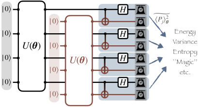
Figure 1: Schematic picture of the joint Bell measurement and JBM-VQE. For an $n$-qubit quantum state $\ket{\psi(\bm{\theta})}=U(\bm{\theta})\ket{0}$, the $2n$-qubit quantum states $\ket{\psi(\bm{\theta})}\otimes\ket{\psi(\bm{\theta})}$ is prepared and measured in the Bell basis. The measurement results can give the estimates of all expectation values $\expectationvalue{P_{j}}_{\bm{\theta}}^{2}=(\expectationvalue{P_{j}}{\psi(\bm{\theta})})^{2}$ in the original $n$-qubit systems, and the state information (energy in JBM-VQE) is estimated by these estimates as well as the pre-given signs of the expectation values.

Noisy intermediate-scale quantum (NISQ) devices [1] have attracted considerable interest as they hold the potential to solve certain computational tasks faster than classical computers [2, 3, 4]. These devices typically have a relatively small number of qubits (usually between 50 and a few hundred) and are subject to hardware noise, so the computational results obtained from them may not be completely reliable. Despite these limitations, NISQ devices are expected to be capable of performing calculations that are beyond the capabilities of classical computers, which makes them exciting tools in the near future. The research community has made substantial progress in developing NISQ-friendly variational quantum optimization algorithms for a variety of applications, including quantum machine learning [5], fidelity estimation [6, 7], quantum error-correcting code discovery [8]. The variational quantum eigensolver (VQE) is considered a flagship algorithm within this field, utilizing parameterized quantum circuits and the variational principle to prepare the ground or excited states of quantum many-body systems [9, 10].

VQE has already been experimentally realized on actual quantum hardware to solve small-sized problems in quantum chemistry and material calculation [9, 11]. However, the scalability of VQE to larger system sizes remains a challenge. One of the main reasons, especially in the application to quantum chemistry, is the large number of measurements required during the optimization process. For the molecular Hamiltonians in quantum chemistry, there are usually $\order{n^{4}}$ Pauli operators for an $n$-qubit system, and estimation of their expectation values is required in each iteration of VQE. For example, it was estimated that a single evaluation of the expectation value of the Hamiltonian for analysing the combustion energies of some organic molecules requires $\sim 10^{9}$ measurement shots and may take as long as several days [12]. To tackle the problem of scalability, various methods have been proposed to reduce the number of measurements in the optimization of VQE. One possible strategy is to divide the $\order{n^{4}}$ Pauli operators in the Hamiltonian into the groups of simultaneously-measurable operators, and there are methods that realize $\mathcal{O}(n^{3})$ groups [13, 14] and even $\mathcal{O}(n^{2})$ groups [15, 16]. The reduction of the number of groups can result in the reduction of the number of measurements to estimate their expectation values, which leads to the alleviation of the scalability problem of VQE. Nonetheless, it is still highly demanded to develop a method to reduce the number of measurements in the whole optimization process of VQE.

Although it is impossible to perform the projective measurement simultaneously on the non-commuting Pauli operators to estimate their expectation values, the absolute values of the expectation values can be estimated simultaneously by using the so-called joint Bell measurement in a doubled system consisting of $2n$ qubits (see Sec. II.2 for detailed explanations). This is because for any $n$-qubit Pauli operators $P_{1},P_{2},\dots,P_{M}$ acting on the original system of $n$ qubit, the operators $P_{1}\otimes P_{1},P_{2}\otimes P_{2},\dots,P_{M}\otimes P_{M}$ acting on the doubled system of $2n$ qubits commute with each other. Then the expectation values of the doubled state $(\bra{\psi}\otimes\bra{\psi})(P_{j}\otimes P_{j})(\ket{\psi}\otimes\ket{\psi})=(\expectationvalue{P_{j}}{\psi})^{2}$ can be estimated simultaneously for all $j=1,\cdots,M$, where $\ket{\psi}$ is a state in the original $n$-qubit system. This joint Bell measurement was utilized to show an exponential advantage of quantum computers over classical ones in predicting properties of physical systems [17, 18] or estimate the reduced density matrix of the quantum state efficiently [19]. It is also noteworthy to point out that the reduction of the number of measurements by a constant factor was achieved in Ref. [20] through the use of Bell measurement. We note that the classical shadow technique [21] also aims at predicting expectation values of many operators simultaneously, but the measurement overhead in the protocol with random Pauli measurements scales exponentially with the locality of the operator, so the application to the quantum chemistry Hamiltonians with non-local Pauli operators is not straightforward (see also Ref. [22]).

In this study, we introduce a method to reduce measurement overhead in VQE by employing joint Bell measurements (JBM), referred to as JBM-VQE (a schematic illustration is provided in Fig. 1). Our approach takes advantage of the correlation between Pauli expectation values across successive iterations of VQE. More concretely, we observe that the signs of expectation values of the Pauli operators in the Hamiltonian change infrequently during the optimization of VQE while their absolute values change frequently. In JBM-VQE, one measures the absolute values by the joint Bell measurement, which requires only one circuit to measure, during every iteration. On the other hand, the signs of expectation values of the Pauli operators are measured once in the fixed number of iterations by the conventional measurement method (using naively $\order{n^{4}}$, at least $\order{n^{2}}$, distinct circuits). The expectation value of the Hamiltonian is subsequently constructed by combining the estimated absolute values and signs with assuming that the latest estimation of the signs is valid for the following iterations. We can expect a reduction in the measurement cost during the optimization by using this protocol. To exemplify this, we numerically compare JBM-VQE to the conventional VQE for molecular Hamiltonians of small molecules under the reasonable condition that the statistical fluctuations of the energy expectation values in both methods are almost the same. JBM-VQE requires fewer shots to approach the vicinity of the exact ground state compared to conventional VQE, with this trend becoming more pronounced for larger molecules. Our proposal is applicable to any molecular Hamiltonian in quantum chemistry and is expected to expedite the practical utilization of VQE. Furthermore, the protocols in JBM-VQE can be utilized in various variational quantum algorithms which optimize the expectation values of many Pauli operators, other than VQE.

The paper is organized as follows. We present the JBM-VQE algorithm in Sec. II. The required number of measurements to estimate the expectation values of the Pauli operators at certain precision is discussed for JBM-VQE and the conventional VQE in Sec. III. The numerical comparison between our proposed JBM-VQE and the conventional VQE on various molecular Hamiltonians is presented in Sec. IV, demonstrating the acceleration of JBM-VQE. We discuss several aspects of JBM-VQE in Sec. V. Finally, we summarize the paper and provide an outlook in Sec. VI.

II Algorithm

In this section, we describe the algorithm of JBM-VQE. We first explain our target Hamiltonian and the joint Bell measurement. We then explain the algorithm of JBM-VQE.

II.1 Setup

We focus on the quantum chemistry Hamiltonian in the second-quantized form, given by

$$H_{\mathrm{f}}=\sum_{i,j=1}^{n}h_{ij}c_{i}^{\dagger}c_{j}+\frac{1}{2}\sum_{i,j,k,l=1}^{n}V_{ijkl}c_{i}^{\dagger}c_{j}^{\dagger}c_{l}c_{k},$$ (1)

where $c_{i}\,(c_{i}^{\dagger})$ is an annihilation (creation) operator of an electron labeled by $i=1,2,\cdots,n$ satisfying the canonical anti-commutation relation $\{c_{i},c_{j}\}=\{c_{i}^{\dagger},c_{j}^{\dagger}\}=0,\{c_{i},c_{j}^{\dagger}\}=\delta_{ij}$, and $h_{ij}\,(V_{ijkl})$ is the scalar related to the so-called one-electron (two-electron) integrals [23, 24]. This Hamiltonian is mapped to a qubit representation by fermion-qubit mappings such Jordan-Wigner mapping [25], parity mapping [26], or Bravyi-Kitaev mapping [27], as follows:

$$H=\sum_{j=1}^{M}\lambda_{j}P_{j},$$ (2)

where $\lambda_{j}\in\mathbb{R}$ is a coefficient, $P_{j}$ is an $n$-qubit Pauli operators $P_{j}\in\{I,X,Y,Z\}^{\otimes n}$, and $M=\order{n^{4}}$ is the number of the Pauli operators. Throughout this paper, we omit the identity term $I^{\otimes n}$ in the Hamiltonian and assume $P_{j}\neq I^{\otimes n}$. Similar to the conventional VQE, JBM-VQE is based on the ansatz quantum state:

$$\ket{\psi(\bm{\theta})}=U(\bm{\theta})\ket{0},$$ (3)

where $U(\bm{\theta})$ is a parameterized quantum circuit with parameters $\bm{\theta}=(\theta_{1},\cdots,\theta_{N_{\theta}})$. Our objective is to minimize the energy expectation value:

$$E(\bm{\theta}):=\expectationvalue{H}_{\bm{\theta}}=\sum_{j=1}^{M}\lambda_{j}\expectationvalue{P_{j}}_{\bm{\theta}},$$ (4)

where $\expectationvalue{\cdots}_{\bm{\theta}}:=\expectationvalue{\cdots}{\psi(\bm{\theta})}$, with respect to the parameters $\bm{\theta}$.

II.2 Joint Bell measurement

The joint Bell measurement enables the determination of the absolute values of expectation values of all $4^{n}$ Pauli operators for an $n$ qubit state [17, 18, 19]. It requires a $2n$-qubit system comprising two identical $n$ qubit systems, denoted as $A$ and $B$. We prepare a $2n$ qubit state,

$$\ket{\Psi(\bm{\theta})}:=\ket{\psi(\bm{\theta})}_{A}\otimes\ket{\psi(\bm{\theta})}_{B}=(U(\bm{\theta})\otimes U(\bm{\theta}))\ket{0}_{A}\otimes\ket{0}_{B},$$ (5)

and apply CNOT gates and Hadamard gates between the corresponding qubits of $A$ and $B$, and eventually measure them in the computational basis (see Fig. 1). For each pair of qubits, measuring the state in the computational basis results in the projective measurement onto the Bell basis,

$$\ket{\Phi_{1}^{\pm}} =\frac{1}{\sqrt{2}}\left(\ket{0}_{A}\otimes\ket{0}_{B}\pm\ket{1}_{A}\otimes\ket{1}_{B}\right),$$ (6)

$$\ket{\Phi_{2}^{\pm}} =\frac{1}{\sqrt{2}}\left(\ket{0}_{A}\otimes\ket{1}_{B}\pm\ket{1}_{A}\otimes\ket{0}_{B}\right).$$

These basis states are common eigenstates of Pauli operators $X_{A}\otimes X_{B}$, $Y_{A}\otimes Y_{B}$, $Z_{A}\otimes Z_{B}$. Therefore, the measurement for all $2n$ qubits in Fig. 1 constitutes the projective measurement on simultaneous eigenstates of all $2n$ qubit Pauli operators in the form of $P_{j}\otimes P_{j}\>(P_{j}\in\{I,X,Y,Z\}^{\otimes n})$, whose total number is $4^{n}$. Consequently, for any $n$ qubit Pauli operators $P_{j}$, we can estimate

$$\expectationvalue{(P_{j}\otimes P_{j})}{\Psi(\bm{\theta})}=\expectationvalue{P_{j}}_{\bm{\theta}}^{2}$$ (7)

from the measurement outcomes of the single quantum circuit in Fig. 1. We denote the estimated value as $\widetilde{\expectationvalue{P_{j}}_{\bm{\theta}}^{2}}$. The absolute value of $\absolutevalue{\expectationvalue{P_{j}}_{\bm{\theta}}}$ is then estimated as

$$\widetilde{\absolutevalue{\expectationvalue{P_{j}}_{\bm{\theta}}}}=\sqrt{\max\{0,\widetilde{\expectationvalue{P_{j}}_{\bm{\theta}}^{2}}\}}.$$ (8)

We refer to this protocol to estimate the absolute values of expectation values of all $4^{n}$ Pauli operators as the joint Bell measurement. We note that the estimate (8) is biased when the number of shots for measurements is finite because of the non-linearity of the square root and the max functions.

II.3 JBM-VQE algorithm

In the JBM-VQE algorithm, we estimate the energy $E(\bm{\theta})$ and its gradient $\partialderivative{E(\bm{\theta})}{\bm{\theta}}$ by decomposing the expectation value $\expectationvalue{P_{j}}_{\bm{\theta}}$ into its sign,

$$s_{j}(\bm{\theta}):=\mathrm{sgn}\left(\expectationvalue{P_{j}}_{\bm{\theta}}\right):=\begin{cases}+1&(\mathrm{if}\expectationvalue{P_{j}}_{\bm{\theta}}\geq 0)\\ -1&(\mathrm{if}\expectationvalue{P_{j}}_{\bm{\theta}}<0)\end{cases},$$ (9)

and its absolute value $\absolutevalue{\expectationvalue{P_{j}}_{\bm{\theta}}}$. We employ the following two subroutines to estimate the energy and gradient in the algorithm.

Subroutine 1. The first subroutine takes the parameters $\bm{\theta}$ as its inputs. In this subroutine, we first estimate the signs $s_{j}(\bm{\theta})$ by evaluating the expectation values $\expectationvalue{P_{j}}_{\bm{\theta}}$ themselves with the standard measurement strategy using $n$ qubits, as done in the conventional VQE. One naive way to estimate the signs is to perform the projective measurement of each $P_{j}$ with $\order{n^{4}}$ distinct measurement circuits, subsequently estimating the sign $s_{j}(\bm{\theta})$ via the majority vote of its $\pm 1$ result. The estimated sign is denoted as $\widetilde{s_{j}(\bm{\theta})}$, and the total number of shots (repetitions of quantum circuit executions) to estimate all $s_{j}(\bm{\theta})$ is represented as $m_{S}^{\text{tot}}$. Following this, the joint Bell measurement using $2n$ qubits is utilized to approximate the absolute values of the expectation values $\absolutevalue{\expectationvalue{P_{j}}_{\bm{\theta}}}$, resulting in their estimates $\widetilde{\absolutevalue{\expectationvalue{P_{j}}_{\bm{\theta}}}}$. The number of shots for the joint Bell measurement is denoted as $m$. The estimate of the energy (expectation value of the Hamiltonian) is constructed as

$$\widetilde{E(\bm{\theta})}=\sum_{j}\lambda_{j}\widetilde{s_{j}(\bm{\theta})}\widetilde{\absolutevalue{\expectationvalue{P_{j}}_{\bm{\theta}}}}.$$ (10)

Additionally, we estimate the gradient of $E(\bm{\theta})$ by using the so-called parameter shift rule [5, 28], mathematically expressed in the simplest case as

$$\partialderivative{\expectationvalue{P_{j}}_{\bm{\theta}}}{\theta_{l}}=\frac{1}{2\sin\alpha}\left(\expectationvalue{P_{j}}_{\bm{\theta}^{(l)}_{+}}-\expectationvalue{P_{j}}_{\bm{\theta}^{(l)}_{-}}\right),$$ (11)

where ${\bm{\theta}}^{(l)}_{\pm}=\bm{\theta}\pm\alpha\bm{\delta}_{l}$, $\bm{\delta}_{l}$ is a unit vector with only the $l$-th component non-zero, and $\alpha\in\mathbb{R}$ is a fixed constant. We take $\alpha=\pi/4$ in the numerical calculation in Sec. IV. Analogous to the energy estimation, we use the standard measurement strategy to estimate the signs $s_{j}(\bm{\theta}^{(l)}_{\pm})$ using the quantum states $\ket{\psi(\bm{\theta}^{(l)}_{\pm})}$, which may require $\order{n^{4}}$ distinct quantum circuits in a naive way. The absolute values $\absolutevalue{\expectationvalue{P_{j}}_{\bm{\theta}^{(l)}_{\pm}}}$ are then estimated with the joint Bell measurement for the states $\ket{\psi(\bm{\theta}^{(l)}_{\pm})}$. The gradient of the energy is estimated by

$$\widetilde{\partialderivative{E(\bm{\theta})}{\theta_{l}}}=\sum_{j}\frac{\lambda_{j}}{2\sin\alpha}\left(\widetilde{s_{j}(\bm{\theta}^{(l)}_{+})}\widetilde{\absolutevalue{\expectationvalue{P_{j}}_{\bm{\theta}^{(l)}_{+}}}}-\widetilde{s_{j}(\bm{\theta}^{(l)}_{-})}\widetilde{\absolutevalue{\expectationvalue{P_{j}}_{\bm{\theta}^{(l)}_{-}}}}\right).$$ (12)

The estimates of the energy (10) and the gradient (12) are the outputs of this subroutine.

Subroutine 2. The second subroutine takes the parameters $\bm{\theta}$ and a set of guessed signs

$$\{t_{j}\}_{j=1}^{M},\> \{t^{(l=1)}_{j,+}\}_{j=1}^{M},\cdots,\{t^{(l=N_{\theta})}_{j,+}\}_{j=1}^{M},$$

$$\{t^{(l=1)}_{j,-}\}_{j=1}^{M},\cdots,\{t^{(l=N_{\theta})}_{j,-}\}_{j=1}^{M},$$ (13)

as inputs ($t_{j},t^{(l)}_{j,\pm}=\pm 1$). In this subroutine, we estimate only the absolute values ($\absolutevalue{\expectationvalue{P_{j}}_{\bm{\theta}}},\absolutevalue{\expectationvalue{P_{j}}_{\bm{\theta}^{(l)}_{+}}}$ and $\absolutevalue{\expectationvalue{P_{j}}_{\bm{\theta}^{(l)}_{-}}}$) by the joint Bell measurement. The energy and the gradient are estimated by

$$\widetilde{E(\bm{\theta})} =\sum_{j}\lambda_{j}t_{j}\widetilde{\absolutevalue{\expectationvalue{P_{j}}_{\bm{\theta}}}}.$$ (14)

$$\widetilde{\partialderivative{E(\bm{\theta})}{\theta_{l}}} =\sum_{j}\frac{\lambda_{j}}{2\sin\alpha}\left(t^{(l)}_{j,+}\widetilde{\absolutevalue{\expectationvalue{P_{j}}_{\bm{\theta}^{(l)}_{+}}}}-t^{(l)}_{j,+}\widetilde{\absolutevalue{\expectationvalue{P_{j}}_{\bm{\theta}^{(l)}_{-}}}}\right).$$ (15)

These two estimates are outputs of the second subroutine.

The JBM-VQE algorithm is described in Algorithm 1. Let us assume that the parameters are $\bm{\theta}$ in the $n_{\mathrm{iter}}$-th iteration ($n_{\mathrm{iter}}=0,1,\cdots$) of the algorithm. When $n_{\mathrm{iter}}$ is a multiple of $T_{S}$, we invoke subroutine 1 to estimate the energy and gradient, $\widetilde{E(\bm{\theta})}$ [Eq. (10)] and $\widetilde{\partialderivative{E(\bm{\theta})}{\bm{\theta}}}$ [Eq. (12)], respectively. Importantly, we also record the estimates of the signs $\widetilde{s_{j}(\bm{\theta})},\widetilde{s_{j,\pm}^{(l)}(\bm{\theta})}$ for $j=1,\cdots,M$ and $l=1,\cdots,N_{\theta}$. When $n_{\mathrm{iter}}$ is not a multiple of $T_{S}$, we invoke subroutine 2 with utilizing the pre-recorded signs (obtained at some past iteration) as the guessed signs [Eq.(13)]. In other words, we estimate the energy and the gradient by Eqs. (14)(15) with performing only the joint Bell measurement that estimates the absolute values of the Pauli expectation values. Then we update the parameters by the gradient decent method $\bm{\theta}^{\prime}=\bm{\theta}-\eta\widetilde{\partialderivative{E(\bm{\theta})}{\bm{\theta}}}$, where $\eta$ is a learning rate. It is worth noting that the gradient descent is not the only choice in the JBM-VQE and other sophisticated optimization algorithms can be employed (see the discussion in Sec. V).

Several remarks regarding our JBM-VQE algorithm are in order. Firstly, this algorithm relies on the expectation that the signs of the Pauli expectation values ($\expectationvalue{P_{j}}_{\bm{\theta}}$ and $\expectationvalue{P_{j}}_{\bm{\theta}^{(l)}_{\pm}}$) do not change frequently during the optimization process. Subroutine 2 consists of the joint Bell measurement that uses only $(2N_{\theta}+1)$ quantum circuits and may typically require fewer measurement shots to estimate the absolute values of the Pauli expectation values than the conventional VQE. For this reason, we expect a reduction in the total number of shots in JBM-VQE compared with the conventional VQE. Secondly, the joint Bell measurement has a bias on its estimates, causing the energy and gradient estimated in both subroutines 1 and 2 to exhibit bias, although this bias will vanish as the number of shots ($m$ and $m_{S}^{\mathrm{tot}}$) approaches infinity. JBM-VQE should be employed when the bias remains relatively small compared to the required energy precision, such as during the early stage of VQE optimization (we discuss this point in Sec. V). The rough criteria of the number of shots for realizing a certain precision of the estimated expectation values are discussed in Sec. III. Thirdly, if we use a $2n$-qubit system just as two independent copies of the original $n$-qubit system and conduct the conventional VQE, $m$ executions of the circuits are equivalent to $2m$ shots in the original system. Consequently, our JBM-VQE algorithm must surpass the conventional VQE by at least a factor of two concerning the number of shots, and it is actually realized in the numerical simulation in Sec. IV. Lastly, the sign-updating period $T_{S}$ influences the efficiency of JBM-VQE. A larger period leads to fewer shots required for optimization, albeit with the trade-off of less accurate energy and gradient estimates. While there is no a priori criterion for determining $T_{S}$, it can be set manually or adaptively by monitoring the optimization history.

Input: Hamiltonian $H=\sum_{j}\lambda_{j}P_{j}$, variational circuit $U(\bm{\theta})$, number of shots for the joint Bell measurement $m$, sign-updating period $T_{S}$, number of shots for sign-updating $m_{S}^{\mathrm{tot}}$, and learning rate $\eta$.

Output: Parameters $\bm{\theta}_{\mathrm{opt}}$ which approximate the ground state of $H$ by $\ket{\psi(\bm{\theta}_{\mathrm{opt}})}=U(\bm{\theta}_{\mathrm{opt}})\ket{0}$ and the estimated optimal energy $\widetilde{E(\bm{\theta})}$.

1 Initialize $\bm{\theta}$ and set $n_{\mathrm{iter}}=0$;

2 while energy estimate $\widetilde{E(\bm{\theta})}$ has not converged do

3       if $n_{\mathrm{iter}}\,\%\,T_{S}=0$ then

4             Call subroutine 1 with input $\bm{\theta}$, and obtain the estimates of the energy [Eq. (10)] and the gradient [Eq. (12)];

5             Record the signs $\widetilde{s_{j}(\bm{\theta})},\widetilde{s_{j,\pm}^{(l)}(\bm{\theta})}$ as $t_{j},t^{(l)}_{j,\pm}$;

6            

7       end if

8      if $n_{\mathrm{iter}}\,\%\,T_{S}\neq 0$ then

9             Call subroutine 2 with input $\bm{\theta}$ and the guessed signs $t_{j},t^{(l)}_{j,\pm}$ at some past iteration, and obtain the estimates of the energy [Eq. (14)] and the gradient [Eq. (15)];

10            

11       end if

12      $\bm{\theta}\leftarrow\bm{\theta}-\eta\widetilde{\partialderivative{E(\bm{\theta})}{\bm{\theta}}}$;

13       $n_{\mathrm{iter}}\leftarrow n_{\mathrm{iter}}+1$;

14      

15 end while

16Return $\bm{\theta}$ and $\widetilde{E(\bm{\theta})}$;

Algorithm 1 JBM-VQE.

III Shot Thresholds

In both JBM-VQE and the conventional VQE, the energy estimate exhibits finite statistical fluctuation due to the limited number of measurement shots. This occurs even without any noise present in quantum devices. To facilitate a fair comparison between JBM-VQE and the conventional VQE, it is essential to establish a common criterion ensuring that both methods display the same level of fluctuation. In this section, we discuss such a criterion by investigating the number of shots required to estimate an expectation value of a single Pauli operator with a fixed level of accuracy. We formulate the number of shots to estimate the expectation value with certain accuracy and probability, and numerically calculate the actual numbers. The number established here is utilized in Sec. IV, where numerical demonstrations of JMB-VQE are performed for quantum chemistry Hamiltonians of small molecules.

III.1 Shot threshold for the conventional VQE

Let us define the number of shots to estimate the expectation value of a single Pauli operator with the projective measurement, which is the standard measurement strategy for the conventional VQE. For a given $n$-qubit state $\ket{\psi}$ and an $n$-qubit Pauli operator $P$, the probability of estimating $\expectationvalue{P}:=\expectationvalue{P}{\psi}$ within an additive error $\tau_{\mathrm{th}}$ under the $m$-shot projective measurement of $P$ is given by

$$p(m,\tau_{\mathrm{th}},\expectationvalue{P}) =\sum_{x=x_{\mathrm{min}}}^{x_{\mathrm{max}}}\binom{m}{x}\left(\frac{1+\expectationvalue{P}}{2}\right)^{x}\left(\frac{1-\expectationvalue{P}}{2}\right)^{m-x},$$ (16)

$$x_{\mathrm{min}} =\mathrm{max}\Big{\{}0,\left\lceil\frac{m(1+\expectationvalue{P}-\tau_{\mathrm{th}})}{2}\right\rceil\Big{\}},$$

$$x_{\mathrm{max}} =\mathrm{min}\Big{\{}m,\left\lfloor\frac{m(1+\expectationvalue{P}+\tau_{\mathrm{th}})}{2}\right\rfloor\Big{\}},$$

where $\lceil...\rceil$ ($\lfloor...\rfloor$) is the ceiling (floor) function of integers. Since there are various Pauli operators included in the Hamiltonian, we consider the averaged probability for estimating the expectation value within an additive error $\tau_{\mathrm{th}}$,

$$p^{(\mathrm{av})}(m,\tau_{\mathrm{th}})=\frac{1}{2}\int_{-1}^{1}dy\,p(m,\tau_{\mathrm{th}},y).$$ (17)

We then define the standard measurement (SM) shot threshold as follows:

Definition 1 (SM shot threshold)

The standard measurement (SM) shot threshold $m^{\mathrm{SM}}_{\mathrm{th}}(\tau_{\mathrm{th}},p_{\mathrm{th}})$ is defined as

$$m_{\mathrm{th}}^{\mathrm{SM}}(\tau_{\mathrm{th}},p_{\mathrm{th}}):=\min\{m\in\mathbb{Z}^{+}\mid p^{(\mathrm{av})}(m,\tau_{\mathrm{th}})\geq p_{\mathrm{th}}\}$$ (18)

The SM shot threshold $m_{\mathrm{th}}^{\mathrm{SM}}(\tau_{\mathrm{th}},p_{\mathrm{th}})$ indicates the minimum number of the shots of the projective measurement of $P$ to estimate $\expectationvalue{P}$ within an additive error $\tau_{\mathrm{th}}$ with a probability at least $p_{\mathrm{th}}$, where the expectation value $\expectationvalue{P}$ is averaged in the uniform distribution for $[-1,1]$. We leverage $m_{\mathrm{th}}^{\mathrm{SM}}(\tau_{\mathrm{th}},p_{\mathrm{th}})$ to determine the number of shots in numerical simulation of the conventional VQE in Sec. IV. We note that the value of $\expectationvalue{P}$ may cluster around $0$ if we consider random states in the Hilbert space, e.g., Haar random states, but we employ the uniform distribution because the ground states of quantum chemistry Hamiltonians are not random states and various values of $\expectationvalue{P}$ may appear.

Finally, we evaluate actual numerical values of $m_{\mathrm{th}}^{\mathrm{SM}}(\tau_{\mathrm{th}},p_{\mathrm{th}})$ for various $\tau_{\mathrm{th}}$ and $p_{\mathrm{th}}$. For a given $m$, we calculate $p^{\mathrm{ave}}(m,\tau_{\mathrm{th}})$ by approximating the integral through numerical integration, taking 2000 uniformly-spaced points of $\expectationvalue{P}$ in the interval $[-1,1]$. The results are presented in Fig. 2.

Figure 2: Values of the standard measurement (SM) shot threshold $m^{\mathrm{SM}}_{\mathrm{th}}(\tau_{\mathrm{th}},p_{\mathrm{th}})$ for different estimation errors $\tau_{\mathrm{th}}$ and probabilities $p_{\mathrm{th}}$.

III.2 Shot threshold for JBM-VQE

In JBM-VQE, the estimation of the absolute value $\expectationvalue{P}$ and the sign $s:=\mathrm{sign}(\expectationvalue{P})$ for a given state $\ket{\psi}$ and a Pauli operator $P$ is performed differently. The absolute value is estimated using joint Bell measurements, while the sign is typically determined through the projective measurement of $P$. We consider the number of shots to estimate each of them within certain error and probability.

First, let us define the number of shots necessary for accurately estimating the absolute value $\expectationvalue{P}$. Since the joint Bell measurement provides the expectation values of $P\otimes P$, the probability of determining $|\langle P\rangle|$ within an error $\tau_{\mathrm{th}}$ is calculated as follows:

$$q(m,\tau_{\mathrm{th}},\expectationvalue{P})$$

$$= \sum_{x\in\mathbb{X}}\binom{m}{x}\left(\frac{1+\expectationvalue{P}^{2}}{2}\right)^{x}\left(\frac{1-\expectationvalue{P}^{2}}{2}\right)^{m-x},$$ (19)

where $\mathbb{X}$ is a set of integers in $0\leq x\leq m$ that satisfies

$$\absolutevalue{\sqrt{\max\big{\{}0,\frac{2x}{m}-1\big{\}}}-\absolutevalue{\expectationvalue{P}}}\leq\tau_{\mathrm{th}}$$ (20)

(see Eq. (8)). Similar to SM shot threshold, we average the probability $q(m,\tau_{\mathrm{th}},\expectationvalue{P})$ as

$$q^{(\mathrm{av})}(m,\tau_{\mathrm{th}})=\frac{1}{2}\int_{-1}^{1}dy\,q(m,\tau_{\mathrm{th}},y).$$ (21)

We can now define JBM shot threshold:

Definition 2 (JBM Shot Threshold)

JBM shot threshold $m^{\mathrm{JBM}}_{\mathrm{th}}(\tau_{\mathrm{th}},p_{\mathrm{th}})$ is defined as

$$m_{\mathrm{th}}^{\mathrm{JBM}}(\tau_{\mathrm{th}},p_{\mathrm{th}}):=\min\{m\in\mathbb{Z}^{+}\mid p^{(\mathrm{av})}(m,\tau_{\mathrm{th}})\geq p_{\mathrm{th}}\}$$ (22)

This means that the JBM shot threshold $m^{\mathrm{JBM}}_{\mathrm{th}}(\tau_{\mathrm{th}},p_{\mathrm{th}})$ indicates the minimal number of shots needed to estimate the absolute value of the expectation value $\expectationvalue{P}$ within an additive error $\tau_{\mathrm{th}}$ with probability $p_{\mathrm{th}}$. Numerical values of $m^{\mathrm{JBM}}_{\mathrm{th}}(\tau_{\mathrm{th}},p_{\mathrm{th}})$ are again calculated by 2000 points of $\expectationvalue{P}$ that are uniformly-spaced in $[-1,1]$ and summarized in Fig. 3.

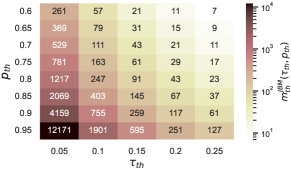
Figure 3: Values of the joint Bell measurement (JBM) shot threshold $m^{\mathrm{JBM}}_{\mathrm{th}}(\tau_{\mathrm{th}},p_{\mathrm{th}})$ for different estimation errors $\tau_{\mathrm{th}}$ and probabilities $p_{\mathrm{th}}$.

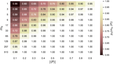
Figure 4: Values of the probability $p_{S}(m_{S},\expectationvalue{P})$ for different measurement shots $m_{S}$ and absolute values of Pauli expectation values $|\langle P\rangle|$.

Next, we examine the estimation of the sign $s$ in JBM-VQE that is performed through a majority vote of the results of the projective measurement of $P$. When the number of shots is an even integer $m_{S}$, the probability of estimating $s$ correctly is

$$p_{S}(m_{S},\expectationvalue{P}) =\sum_{x\in\mathbb{X}_{S}}\binom{m_{S}}{x}\left(\frac{1+\expectationvalue{P}}{2}\right)^{x}\left(\frac{1-\expectationvalue{P}}{2}\right)^{m_{S}-x},$$ (23)

$$\mathbb{X}_{S} =\begin{cases}\{\frac{m_{S}}{2},\frac{m_{S}}{2}+1,\cdots,m_{S}\}&(\expectationvalue{P}\geq 0)\\ \{0,1,\cdots,\frac{m_{S}}{2}-1\}&(\expectationvalue{P}<0)\end{cases}$$ (24)

The numerical values of $p_{S}(m_{S},\langle P\rangle)$ are presented in Fig. 4. We observe that even for a relatively small number of shots such as $m_{S}=17$, the probability $p^{\prime}$ is as high as $\geq 0.8$ for $\expectationvalue{P}\geq 0.2$. In our numerical simulations presented in the next section, we take these values into account for determining the value of $m_{S}$ in the JBM-VQE algorithm.

Finally, it is worthwhile to point out that $m_{\mathrm{th}}^{\mathrm{SM}}$ and $m_{S}$ considered here are defined for a single Pauli operator $P$, so if there are $M$ Pauli operators, it would require $M\cdot m_{\mathrm{th}}^{\mathrm{SM}}$ and $M\cdot m_{S}$ shots to estimate all expectation values and their sign. Similarly, it is shown [18] that $\order{\log(M)/\epsilon^{4}}$ measurements are need to estimate $\absolutevalue{\expectationvalue{P_{1}}},\cdots,\absolutevalue{\expectationvalue{P_{M}}}$ within the error $\epsilon$ simultaneously, so it would require $\log(M)\cdot m_{\mathrm{th}}^{\mathrm{JBM}}$ to estimate all absolute values of them.

IV Numerical demonstration

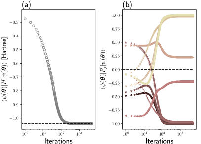
Figure 5: Expectation values of (a) the Hamiltonian $H$ and (b) the Pauli operators $P_{j}$ included in the Hamiltonian during the VQE optimization for finding the ground state of the H2 molecular Hamiltonian. There are 14 non-identity Pauli operators included in the Hamiltonian $H$.

In this section, we present numerical demonstrations of JBM-VQE for finding the ground states of quantum chemistry Hamiltonians. We first examine an example where the signs of Pauli expectation values, $s_{j}(\bm{\theta})$, do not undergo frequent flipping during the course of standard VQE optimization. This observation leads to the anticipation that JBM-VQE can reduce the number of shots to optimize the parameters with a specified level of accuracy. We then compare JBM-VQE and the conventional VQE by taking various small molecules as examples. The parameter optimization in JBM-VQE proceeds more rapidly than in the conventional VQE, according to the metric we have established for the early stage of the optimization. The advantage of JBM-VQE becomes increasingly apparent as system sizes (the number of qubits) grow larger.

IV.1 Signs of Pauli expectation values during parameter optimization

We conduct a numerical simulation of the conventional VQE to prepare the ground state of the $\ce{H2}$ molecular Hamiltonian whose bond distance is 0.74Å. The quantum chemistry Hamiltonian of the form (1) is constructed by using the Hartree-Fock molecular orbitals with the STO-3G basis set. The Hamiltonian is then mapped to the qubit form (2) via the Jordan-Wigner transformation. The resulting qubit Hamiltonian consists of $n=4$ qubits and 14 non-identity Pauli operators. The construction of the Hamiltonian was implemented using the numerical libraries PySCF [29] and OpenFermion [30]. For the VQE ansatz state, we employ the symmetry-preserving ansatz [31, 32] $\ket{\psi(\bm{\theta})}=U(\bm{\theta})\ket{n_{e}}$, where $U(\bm{\theta})$ represents a variational quantum circuit depicted in Fig. 7 of Appendix A and $\ket{n_{e}}$ is a computational basis state $\ket{0\cdots 01\cdots 1}$ with $n-n_{e}$ “0”s and $n_{e}$ “1”s with $n_{e}$ denoting the number of electrons (for H2 molecule, $n_{e}=2$). It has eight parameters in total, with initial values sampled randomly from $[0,\pi/5]$. The parameters are updated using the gradient descent method with a learning rate $\eta=0.02$. We simulate the energy expectation values $E(\bm{\theta})=\expectationvalue{H}{\psi(\bm{\theta})}$ exactly without assuming any statistical error and noise sources by the numerical library Qulacs [33].

The result is presented in Fig. 5. After 3000 iterations, the VQE algorithm successfully finds the exact ground state. Importantly, we observe that the signs of the expectation values of the most Pauli operators $\expectationvalue{P_{j}}{\psi(\bm{\theta})}$ either remain unchanged or exhibit only a single change during the VQE optimization. This observation motivates us to accelerate VQE by estimating only the absolute values of $\expectationvalue{P_{j}}{\psi(\bm{\theta})}$ in the majority of iterations. We note that expectation values of some Pauli operators (e.g., $\langle X_{1}\otimes Y_{2}\otimes Y_{3}\otimes X_{4}\rangle$ and $\langle Y_{1}\otimes X_{2}\otimes X_{3}\otimes Y_{4}\rangle$) are the same throughout the optimization process due to the ansatz symmetry.

IV.2 Comparison of JBM-VQE with the conventional VQE for various small molecules

Here we present a numerical comparison of the measurement cost between JBM-VQE and the conventional VQE. We consider eight molecular systems: H2, H3+, H4, H5+, LiH, H2O, NH3, and BeH2. The geometries of these molecules are provided in Table 1 of Appendix A. For the latter four molecules (LiH, H2O, NH3, and BeH2), the active space approximation of four orbitals are taken so that the Hamiltonians become 8-qubit ones.

Similar to the calculations in the previous subsection, we construct quantum chemistry Hamiltonians of the form (1) using Hartree-Fock molecular orbitals with the STO-3G basis set for the eight molecules under consideration. The Jordan-Wigner transformation is employed to obtain the qubit Hamiltonian. The symmetry-preserving ansatz (described in Fig. 7 of Appendix A) is employed for both JBM-VQE and the conventional VQE. The ansatz depths for molecules H2, H3+, H4, H5+, LiH, H2O, NH3, and BeH2 are 2, 3, 8, 14, 3, 5, 6, and 5, respectively. Initial parameters are uniformly sampled from $[0,\pi/5]$ for all cases.

We evaluate the expectation value $E(\bm{\theta})=\expectationvalue{H}{\psi(\bm{\theta})}$ and its gradient as follows. In JBM-VQE, the signs $\{s_{j}(\bm{\theta})\}_{j=1}^{M}$ and $\{s_{j}(\bm{\theta}^{(l)}_{\pm})\}_{j=1}^{M}$ are estimated by the projective measurement of the Pauli operators $P_{j}$ included in the Hamiltonian. We employ the qubit-wise commuting (QWC) grouping [11, 34] to make groups of simultaneously-measurable Pauli operators, which requires additional $\order{n}$ one-qubit gates and reduces the number of the total shots for estimation (see Appendix A for details). We allocate the same number of shots for all generated groups, denoting the number of shots for each group as $m_{S}$. The absolute values $\{\absolutevalue{\expectationvalue{P_{j}}_{\bm{\theta}}}\}_{j=1}^{M}$ are estimated using the joint Bell measurement with $2n$ qubits, as described in Sec. II. The number of shots for the joint Bell measurement is denoted by $m$. In the conventional VQE, we estimate the energy expectation value by directly estimating $\expectationvalue{P_{j}}{\psi(\bm{\theta})}$ with the projective measurement of $P_{j}$. We also employ QWC grouping to reduce the number of shots and allocate the same amount of shots for all groups. The number of shots for each group is denoted by $m_{\mathrm{VQE}}$. For both JBM-VQE and the conventional VQE, all outcomes of the measurement shots (bitstrings) are simulated without considering any noise sources using the numerical library Qulacs [33].

The learning parameter for the gradient descent is set to $\eta=0.02$ for both JBM-VQE and the conventional VQE. As mentioned in Sec. II, we set $\alpha=\pi/4$ in the parameter shift rule (11) to estimate the gradient because of the reason described in Appendix A. We consider the threshold of $p_{\mathrm{th}}=0.9$ and $\tau_{\mathrm{th}}=0.05$ for estimating the Pauli expectation values. According to Figs. 2, 3 and 4, the numbers of the shots are taken as $m=4159$, $m_{S}=513$, and $m_{\mathrm{VQE}}=739$. Note that the standard deviations (or fluctuations) in estimating the energy expectation values are not strictly the same between JBM-VQE and the conventional VQE because the values of the thresholds discussed in Sec. III are for a single Pauli operator. The sign-updating period of JBM-VQE is fixed at $T_{S}=30$ for all simulations. For every 200 iterations, the mean estimated energy is computed. Should the energy fail to decrease by a minimum of $0.001$ following $200$ iterations, the optimization process is terminated.

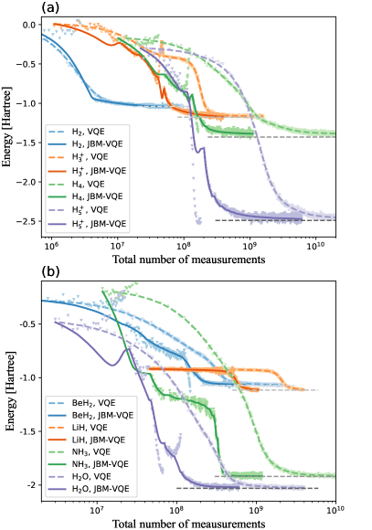
Figure 6: Comparison of optimization curves for the conventional VQE and the JBM-VQE algorithms applied to molecular Hamiltonians of (a) $\ce{H2}$, $\ce{H3+}$, $\ce{H4}$, $\ce{H5+}$ and (b) $\ce{LiH}$, $\ce{H2O}$, $\ce{NH3}$, and $\ce{BeH2}$. The solid lines and circles denote the actual energy (exact energy expectation value for the parameters at each iteration) and the estimated energy in the conventional VQE, respectively. The dashed lines and triangles represent the actual energy and the estimated energy in JBM-VQE, respectively.

The results are shown in Fig. 6. For all molecules, JBM-VQE exhibits a faster decrease of energy with fewer measurement shots. The sudden jump of the estimated energy in JBM-VQE appears to be due to the update of the signs. It is also observed that the advantage of JBM-VQE becomes more evident as the system size increases from 4 qubits (H2) to 10 qubits (H5+). To quantify the improvement of the measurement cost of JBM-VQE over the conventional VQE, we count the number of the shots required to achieve a result with energy lower than the Hartree-Fock energy. The ratio between such shots for the conventional VQE over JBM-VQE is calculated by averaging the results of at least 50 independent numerical simulations with different initial parameters, which yields ($n$ denotes the number of qubits)

$$\ce{H2}(n=4):1.44, \ce{H3+}(n=6):3.45,$$ (25)

$$\ce{H4}(n=8):9.00, \ce{H5+}(n=10):9.24,$$

$$\ce{BeH2}(n=8):3.70, \ce{LiH}(n=8):4.60,$$

$$\ce{NH3}(n=8):11.60, \ce{H2O}(n=8):2.24.$$

These numbers illustrate the reduction of the measurement cost of JBM-VQE.

Finally, we comment on the choice of the Hartree-Fock energy to define the number of shots for optimizing the parameters of the ansatz although the Hartree-Fock energy can be obtained by the initial state of the ansatz without applying $U(\bm{\theta})$. This is because the purpose of this numerical illustration is to simply show the reduction of the number of shots in the optimization process of (JBM-)VQE. Furthermore, it is important to acknowledge that the ansatz selected in this study does not guarantee the accurate representation of the ground-state for the given Hamiltonian. This limitation arises due to the expressibility constraints of the ansatz and make it difficult to define the number of shots for the optimization by using the exact ground state energy.

V Discussion

In this section, we discuss several aspects of the JBM-VQE method.

First, JBM-VQE can be expected to present a significant advantage over conventional VQE as the number of qubits $n$ increases, as demonstrated in the hydrogen chain examples from the previous section. This is because the number of distinct quantum circuits to evaluate the energy expectation value scales at least $\order{n^{2}}$ (naively $\order{n^{4}}$) in the conventional VQE while that of JBM-VQE does $\order{1}$ when we skip the evaluation of the sign of the Pauli expectation values. Although a small number of distinct quantum circuits does not directly imply the efficiency of the evaluation, we anticipate a reduction of the total number of shots in JBM-VQE, as illustrated in the previous section.

Second, we propose using JBM-VQE as an initial optimizer when the accuracy of the energy estimate is not as high, as demonstrated in the numerical simulation in Sec. IV, because of the following two reasons. The first reason is that the estimate of the energy in JBM-VQE is biased, i.e., the average of $\widetilde{E(\bm{\theta})}$ (Eqs. (10)(14)) is not equal to the true value $E(\bm{\theta})$ (note that the estimate $\widetilde{E(\bm{\theta})}$ is a random variable whose probability distribution is determined by that of the outcomes of the joint Bell measurement). The bias has already been seen in the numerical simulation (Fig. 6), where the distribution of the dots (the energy estimates) is not centered at the corresponding line (the exact value of the energy at those parameters) for several molecules. The second reason is the scaling of the number of shots in the joint Bell measurement with respect to the estimation error. As shown in Ref. [18], the number of shots required to estimate all $M$ absolute values $\absolutevalue{\expectationvalue{P_{1}}},\cdots,\absolutevalue{\expectationvalue{P_{M}}}$ with the error $\epsilon$ by the joint Bell measurement is $\order{\log(M)/\epsilon^{4}}$. This $\epsilon^{-4}$ scaling can be problematic when we take small $\epsilon$. These two properties of JBM-VQE can pose challenges when optimizing the ansatz parameters with high accuracy required quantum chemistry, such as the so-called chemical accuracy $10^{-3}$ Hartree.

Third, we point out that the JBM-VQE protocol is flexible and can be combined with various variational algorithms which require the evaluation of many Pauli expectation values to optimize the parameters. For example, sophisticated optimizers like Adam [35] or the ones more tailored for VQE [36, 37] can be used in JBM-VQE although we employ the plain-vanilla gradient decent in the numerical simulations. One can simply skip the evaluation of the signs of Pauli expectation values at some iterations (parameter updates) and perform the joint Bell measurement to estimate the energy and its gradient that are fed into the optimizers.

VI Summary and Outlook

In this study, we introduce a protocol designed to accelerate the Variational Quantum Eigensolver (VQE) algorithm for determining the ground state of molecular Hamiltonians. Our approach employs the joint Bell measurement to estimate the energy expectation value and its gradient of $n$ qubit systems with $\order{n^{0}}=\order{1}$ distinct quantum circuits in the majority of iterations, under the assumption that the signs of Pauli expectation values do not frequently change during optimization. In contrast, the conventional VQE necessitates at least $\mathcal{O}(n^{2})$ distinct quantum circuits for estimating the energy and gradient in each iteration. We conducted numerical simulations of various small molecular Hamiltonians, demonstrating that our proposed protocol effectively reduces the number of measurement shots required to optimize the ansatz parameters to a certain level. JBM-VQE holds promise for application in a broad range of near-term quantum algorithms that depend on Pauli expectation value estimations.

In future work, it is interesting to apply our protocol to various NISQ algorithms other than the simple VQE presented in this study. For example, it is possible to combine JBM-VQE with the variants of VQE for excited states [38, 39], quantum imaginary-time evolution [40, 41, 42, 43], and algorithmic error mitigation schemes [44, 45]. There is reason to believe that in protocols involving estimating quantum computed moments $\langle\psi|H^{k}|\psi\rangle$ like the Lanczos-inspired error mitigation scheme [45], variance-VQE (where $k=2$) [46], and variance extrapolation [44], the acceleration from joint Bell measurement become more significant since the number of Pauli terms to be evaluated is of order $\mathcal{O}(n^{4k})$. Furthermore, it would be beneficial to explore the integration of our protocol with two notable strategies - the $\alpha$-VQE [47] and the parallelized VQE [48]. Both of these approaches have demonstrated promising results in improving the efficiency of VQE optimization.

Appendix A Details of numerical calculation

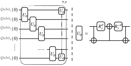
Figure 7: Left: The symmetry preserving real-valued ansatz with $n$ qubits and $p$ layers for constructing the ground state of a molecular Hamiltonian. Right: The $\mathrm{SO}(4)$ block with three CNOT gates and two $R_{y}$ rotations with opposite rotation angles.

Table 1: Geometries and active spaces (if any) of molecules. $n$ is the number of qubits of the molecular Hamiltonian. “$(\mathrm{X},(x,y,z))$” denotes three dimensional coordinates $x,y,z$ of atom X in units of Å.

Molecule (active space)	$n$	Geometry
H2	4	(H, (0, 0, 0)), (H, (0, 0, 0.74))
H3+	6	(H, (0, 0, 0)), (H, (0, 0, 0.85)), (H, (0, 0.74, 0.43))
H4	8	(H, (0, 0, 0)), (H, (0, 0, 1.2)), (H, (0, 0, 2.4)), (H, (0, 0, 3.6))
H5+	10	(H, (0, 0, 0)), (H, (0, 0.74, 0.43)), (H, (0, 0.74, -0.43)), (H, (-0.74, 0, 0.43)), (H, (-0.74, 0, -0.43))
LiH(4o,2e)	8	(Li, (0, 0, 0)), (H, (0, 0, 1.59))
H2O(4o,4e)	8	(O, (0, 0, 0.137)), (H, (0,0.76,0.50)), (H, (0,-0.76,-0.50))
NH3(4o,4e)	8	(N, (0,0,0)), (H, (0, 0, 1.01)), (H, (0.95, 0, -0.34)), (H, (-0.48, -0.82, -0.34))
BeH2(4o,4e)	8	(Be, (0, 0, 0)), (H, (0, 0, 1.33)), (H, (0, 0, -1.33))

A.1 Details of ansatz and molecules

In the numerical simulations presented in Sec. IV, we employ the symmetry-preserving real-valued ansatz depicted in Fig. 7. We use molecules with geometries and active spaces listed in Table 1. Some of these geometries are chosen as the stable structures at the level of Hartree-Fock/STO-3G, as referenced from the CCCBDB database.

A.2 Qubit wise commuting grouping

For the numerical simulations shown in Fig. 6, we employ the qubit-wise commuting (QWC) grouping [11, 34] to evaluate the expectation values of the Hamiltonian $H$. Consider two $n$-qubit Pauli operators, $Q_{1}=\sigma_{1}^{(1)}\otimes\sigma_{1}^{(2)}\otimes\dots\otimes\sigma_{1}^{(n)}$ and $Q_{2}=\sigma_{2}^{(1)}\otimes\sigma_{2}^{(2)}\otimes\dots\otimes\sigma_{2}^{(n)}$, where $\sigma_{1,2}^{(j)}$ is a single qubit Pauli operator $I,X,Y,Z$ acting on $j$-th qubit. We define that $Q_{1}$ and $Q_{2}$ are qubit-wise commuting if and only if $\sigma_{1}^{(j)}\sigma_{2}^{(j)}=\sigma_{2}^{(j)}\sigma_{1}^{(j)}$ for all $j\in\{1,2,\dots,n\}$. The Pauli operators $\{Q_{1},Q_{2},\cdots\}$ that are mutually qubit-wise commuting can be simultaneously measured by applying an additional quantum circuit consisting of $O(n)$ one-qubit gates to the state $\ket{\psi}$. Therefore, we can reduce the number of distinct quantum circuit to evaluate the expectation value of the Hamiltonian $H=\sum_{j=1}^{M}\lambda_{j}P_{j}$ by dividing the Pauli operators $\{P_{j}\}_{j=1}^{M}$ into groups of mutually qubit-wise commuting operators. It should be noted that various grouping methods have been explored in the literature, including those considering usual commutativity and anti-commutativity of the Pauli operators [49, 50, 51, 52, 53]. The QWC grouping method is adopted in our simulation because it does not require deep and complicated quantum circuits to perform simultaneous measurements of the operators in each group.

The greedy search with sorting the Pauli operators [54] is employed when grouping the Pauli operators included in the Hamiltonian. We sort the $M$ Pauli operators $\{P_{j}\}_{j=1}^{M}$ in the Hamiltonian by descending order of the absolute values of the coefficients $|\lambda_{j}|$. The sorted operators are denoted $\{P^{\prime}_{j}\}_{j=1}^{M}$. We assign $P^{\prime}_{1}$ to the first group. For $j=2,3,\dots,k$, if $P^{\prime}_{j}$ qubit-wise commutes with all Pauli operators in an existing group, it is assigned to that group. If $P^{\prime}_{j}$ does not qubit-wise commute with any Pauli operators in an existing group, a new group is created to house $P^{\prime}_{j}$. This procedure is repeated until all Pauli operators are assigned to a group.

A.3 Choice of $\alpha$ in parameter-shift rule

Here, we explain the choice of $\alpha=\pi/4$ in the parameter shift rule (11) in our numerical calculation. The parameter shift rule is related to the fact [55] that the functional form of the Pauli expectation value with respect to $\theta_{l}$ is a trigonometric function when other circuit parameters remain constant: in the simplest cases where the parameter $\theta_{l}$ in the ansatz $\ket{\psi(\bm{\theta})}$ is an angle of some Pauli rotation gate $e^{-i\frac{\theta_{l}}{2}Q_{l}}$ satisfying $Q_{l}^{2}=I$, we have

$$\expectationvalue{P_{j}}_{\bm{\theta}}=a_{l}\cos\left(\theta_{l}-\phi_{l}\right)+c_{l},$$ (26)

where $a_{l},\phi_{l}$ and $c_{l}$ are real coefficients depending on $\theta_{1},\cdots,\theta_{l-1},\theta_{l+1},\cdots,\theta_{N_{\theta}}$. The parameter shift rule can improve the signal-to-noise ratio when we take larger $\alpha$. For example, if we use small $\alpha$ like $\alpha=0.01$, the values $\expectationvalue{P_{j}}_{\bm{\theta}+\alpha\delta_{l}}$ and $\expectationvalue{P_{j}}_{\bm{\theta}-\alpha\delta_{l}}$ become almost the same so that a lot of measurement shots are required to estimate the gradient ($\propto\expectationvalue{P_{j}}_{\bm{\theta}+\alpha\delta_{l}}-\expectationvalue{P_{j}}_{\bm{\theta}-\alpha\delta_{l}}$) with high accuracy. This is why $\alpha=\pi/2$, the largest $\alpha$ considering the periodicity of the function (26), is typically used in the literature [5]. In our numerical calculation, we observed that some Pauli terms exhibit expectation values approaching $\expectationvalue{P_{j}}_{\bm{\theta}}\approx\pm 1$ in the late stages of optimization, or at the vicinity of the exact ground state. For these Pauli terms, $\absolutevalue{\expectationvalue{P_{j}}_{\bm{\theta}\pm(\pi/2)\delta_{l}}}$ sometimes becomes close to zero (e.g., when $a_{l}=1$, $c_{l}=0$ in (26)) and the estimation of it by the joint Bell measurement requires a large number of shots (see Table 3). Consequently, to strike a balance, we adopt $\alpha=\pi/4$ for our numerical computations presented in Sec. IV. In fact, for Pauli terms satisfying $\expectationvalue{P_{j}}_{\bm{\theta}}=\pm 1$, $\absolutevalue{\expectationvalue{P_{j}}_{\bm{\theta}\pm\pi/4\delta_{l}}}$ is farther away from zero than $\absolutevalue{\expectationvalue{P_{j}}_{\bm{\theta}\pm\pi/2\delta_{l}}}$ and guaranteed to be larger than $\frac{\sqrt{2}}{2}$,

$$\absolutevalue{\expectationvalue{P_{j}}_{\bm{\theta}\pm\pi/2\delta_{l}}}=\absolutevalue{a_{l}\cdot\frac{\sqrt{2}}{2}+c_{l}}\geq\frac{\sqrt{2}}{2},$$ (27)

because $|a_{l}|\leq 1$ and $|a_{l}|+|c_{l}|\leq 1$ hold due to $\absolutevalue{\expectationvalue{P_{j}}_{\bm{\theta}}}\leq 1$ for any $\bm{\theta}$.

References

- Preskill [2018] J. Preskill, Quantum Computing in the NISQ era and beyond, Quantum 2, 79 (2018).
- Arute et al. [2019] F. Arute, K. Arya, R. Babbush, D. Bacon, J. C. Bardin, R. Barends, R. Biswas, S. Boixo, F. G. Brandao, D. A. Buell, et al., Quantum supremacy using a programmable superconducting processor, Nature 574, 505 (2019).
- Zhong et al. [2020] H.-S. Zhong, H. Wang, Y.-H. Deng, M.-C. Chen, L.-C. Peng, Y.-H. Luo, J. Qin, D. Wu, X. Ding, Y. Hu, et al., Quantum computational advantage using photons, Science 370, 1460 (2020).
- Madsen et al. [2022] L. S. Madsen, F. Laudenbach, M. F. Askarani, F. Rortais, T. Vincent, J. F. Bulmer, F. M. Miatto, L. Neuhaus, L. G. Helt, M. J. Collins, et al., Quantum computational advantage with a programmable photonic processor, Nature 606, 75 (2022).
- Mitarai et al. [2018] K. Mitarai, M. Negoro, M. Kitagawa, and K. Fujii, Quantum circuit learning, Phys. Rev. A 98, 032309 (2018).
- Cerezo et al. [2020] M. Cerezo, A. Poremba, L. Cincio, and P. J. Coles, Variational Quantum Fidelity Estimation, Quantum 4, 248 (2020).
- Chen et al. [2021] R. Chen, Z. Song, X. Zhao, and X. Wang, Variational quantum algorithms for trace distance and fidelity estimation, Quantum Science and Technology 7, 015019 (2021).
- Cao et al. [2022a] C. Cao, C. Zhang, Z. Wu, M. Grassl, and B. Zeng, Quantum variational learning for quantum error-correcting codes, Quantum 6, 828 (2022a).
- Peruzzo et al. [2014] A. Peruzzo, J. McClean, P. Shadbolt, M.-H. Yung, X.-Q. Zhou, P. J. Love, A. Aspuru-Guzik, and J. L. O’Brien, A variational eigenvalue solver on a photonic quantum processor, Nature Communications 5, 4213 (2014).
- Tilly et al. [2022] J. Tilly, H. Chen, S. Cao, D. Picozzi, K. Setia, Y. Li, E. Grant, L. Wossnig, I. Rungger, G. H. Booth, and J. Tennyson, The variational quantum eigensolver: A review of methods and best practices, Physics Reports 986, 1 (2022).
- Kandala et al. [2017] A. Kandala, A. Mezzacapo, K. Temme, M. Takita, M. Brink, J. M. Chow, and J. M. Gambetta, Hardware-efficient variational quantum eigensolver for small molecules and quantum magnets, Nature 549, 242 (2017).
- Gonthier et al. [2022] J. F. Gonthier, M. D. Radin, C. Buda, E. J. Doskocil, C. M. Abuan, and J. Romero, Measurements as a roadblock to near-term practical quantum advantage in chemistry: Resource analysis, Phys. Rev. Res. 4, 033154 (2022).
- Gokhale et al. [2020] P. Gokhale, O. Angiuli, Y. Ding, K. Gui, T. Tomesh, M. Suchara, M. Martonosi, and F. T. Chong, measurement cost for variational quantum eigensolver on molecular hamiltonians, IEEE Transactions on Quantum Engineering 1, 1 (2020).
- Zhao et al. [2020a] A. Zhao, A. Tranter, W. M. Kirby, S. F. Ung, A. Miyake, and P. J. Love, Measurement reduction in variational quantum algorithms, Phys. Rev. A 101, 062322 (2020a).
- Bonet-Monroig et al. [2020] X. Bonet-Monroig, R. Babbush, and T. E. O’Brien, Nearly optimal measurement scheduling for partial tomography of quantum states, Phys. Rev. X 10, 031064 (2020).
- Inoue et al. [2023] W. Inoue, K. Aoyama, Y. Teranishi, K. Kanno, Y. O. Nakagawa, and K. Mitarai, Almost optimal measurement scheduling of molecular hamiltonian via finite projective plane (2023), arXiv:2301.07335 [quant-ph] .
- Huang et al. [2022] H.-Y. Huang, M. Broughton, J. Cotler, S. Chen, J. Li, M. Mohseni, H. Neven, R. Babbush, R. Kueng, J. Preskill, and J. R. McClean, Quantum advantage in learning from experiments, Science 376, 1182 (2022).
- Huang et al. [2021] H.-Y. Huang, R. Kueng, and J. Preskill, Information-theoretic bounds on quantum advantage in machine learning, Phys. Rev. Lett. 126, 190505 (2021).
- Jiang et al. [2020] Z. Jiang, A. Kalev, W. Mruczkiewicz, and H. Neven, Optimal fermion-to-qubit mapping via ternary trees with applications to reduced quantum states learning, Quantum 4, 276 (2020).
- Hamamura and Imamichi [2020] I. Hamamura and T. Imamichi, Efficient evaluation of quantum observables using entangled measurements, npj Quantum Information 6, 56 (2020).
- Huang et al. [2020] H.-Y. Huang, R. Kueng, and J. Preskill, Predicting many properties of a quantum system from very few measurements, Nature Physics 16, 1050 (2020).
- Zhao et al. [2021] A. Zhao, N. C. Rubin, and A. Miyake, Fermionic partial tomography via classical shadows, Phys. Rev. Lett. 127, 110504 (2021).
- Szabo and Ostlund [2012] A. Szabo and N. S. Ostlund, Modern quantum chemistry: introduction to advanced electronic structure theory (Courier Corporation, 2012).
- Helgaker et al. [2013] T. Helgaker, P. Jorgensen, and J. Olsen, Molecular electronic-structure theory (John Wiley & Sons, 2013).
- Jordan and Wigner [1928] P. Jordan and E. Wigner, Über das paulische äquivalenzverbot, Zeitschrift für Physik 47, 631 (1928).
- Seeley et al. [2012] J. T. Seeley, M. J. Richard, and P. J. Love, The bravyi-kitaev transformation for quantum computation of electronic structure, The Journal of Chemical Physics 137, 224109 (2012).
- Bravyi and Kitaev [2002] S. B. Bravyi and A. Y. Kitaev, Fermionic quantum computation, Annals of Physics 298, 210 (2002).
- Schuld et al. [2019] M. Schuld, V. Bergholm, C. Gogolin, J. Izaac, and N. Killoran, Evaluating analytic gradients on quantum hardware, Phys. Rev. A 99, 032331 (2019).
- Sun et al. [2018] Q. Sun, T. C. Berkelbach, N. S. Blunt, G. H. Booth, S. Guo, Z. Li, J. Liu, J. D. McClain, E. R. Sayfutyarova, S. Sharma, S. Wouters, and G. K.-L. Chan, Pyscf: the python-based simulations of chemistry framework, WIREs Computational Molecular Science 8, e1340 (2018).
- McClean et al. [2020] J. R. McClean, N. C. Rubin, K. J. Sung, I. D. Kivlichan, X. Bonet-Monroig, Y. Cao, C. Dai, E. S. Fried, C. Gidney, B. Gimby, P. Gokhale, T. Häner, T. Hardikar, V. Havlíček, O. Higgott, C. Huang, J. Izaac, Z. Jiang, X. Liu, S. McArdle, M. Neeley, T. O’Brien, B. O’Gorman, I. Ozfidan, M. D. Radin, J. Romero, N. P. D. Sawaya, B. Senjean, K. Setia, S. Sim, D. S. Steiger, M. Steudtner, Q. Sun, W. Sun, D. Wang, F. Zhang, and R. Babbush, Openfermion: the electronic structure package for quantum computers, Quantum Science and Technology 5, 034014 (2020).
- Gard et al. [2020] B. T. Gard, L. Zhu, G. S. Barron, N. J. Mayhall, S. E. Economou, and E. Barnes, Efficient symmetry-preserving state preparation circuits for the variational quantum eigensolver algorithm, npj Quantum Information 6, 10 (2020).
- Ibe et al. [2022] Y. Ibe, Y. O. Nakagawa, N. Earnest, T. Yamamoto, K. Mitarai, Q. Gao, and T. Kobayashi, Calculating transition amplitudes by variational quantum deflation, Phys. Rev. Res. 4, 013173 (2022).
- Suzuki et al. [2021] Y. Suzuki, Y. Kawase, Y. Masumura, Y. Hiraga, M. Nakadai, J. Chen, K. M. Nakanishi, K. Mitarai, R. Imai, S. Tamiya, T. Yamamoto, T. Yan, T. Kawakubo, Y. O. Nakagawa, Y. Ibe, Y. Zhang, H. Yamashita, H. Yoshimura, A. Hayashi, and K. Fujii, Qulacs: a fast and versatile quantum circuit simulator for research purpose, Quantum 5, 559 (2021).
- Verteletskyi et al. [2020] V. Verteletskyi, T.-C. Yen, and A. F. Izmaylov, Measurement optimization in the variational quantum eigensolver using a minimum clique cover, The Journal of Chemical Physics 152, 124114 (2020).
- Kingma and Ba [2017] D. P. Kingma and J. Ba, Adam: A method for stochastic optimization (2017), arXiv:1412.6980 [cs.LG] .
- Kübler et al. [2020] J. M. Kübler, A. Arrasmith, L. Cincio, and P. J. Coles, An Adaptive Optimizer for Measurement-Frugal Variational Algorithms, Quantum 4, 263 (2020).
- Arrasmith et al. [2020] A. Arrasmith, L. Cincio, R. D. Somma, and P. J. Coles, Operator sampling for shot-frugal optimization in variational algorithms (2020), arXiv:2004.06252 [quant-ph] .
- Nakanishi et al. [2019] K. M. Nakanishi, K. Mitarai, and K. Fujii, Subspace-search variational quantum eigensolver for excited states, Phys. Rev. Res. 1, 033062 (2019).
- Parrish et al. [2019] R. M. Parrish, E. G. Hohenstein, P. L. McMahon, and T. J. Martínez, Quantum computation of electronic transitions using a variational quantum eigensolver, Phys. Rev. Lett. 122, 230401 (2019).
- Motta et al. [2020] M. Motta, C. Sun, A. T. K. Tan, M. J. O’Rourke, E. Ye, A. J. Minnich, F. G. S. L. Brandão, and G. K.-L. Chan, Determining eigenstates and thermal states on a quantum computer using quantum imaginary time evolution, Nature Physics 16, 205 (2020).
- McArdle et al. [2019] S. McArdle, T. Jones, S. Endo, Y. Li, S. C. Benjamin, and X. Yuan, Variational ansatz-based quantum simulation of imaginary time evolution, npj Quantum Information 5, 75 (2019).
- Sun et al. [2021] S.-N. Sun, M. Motta, R. N. Tazhigulov, A. T. Tan, G. K.-L. Chan, and A. J. Minnich, Quantum computation of finite-temperature static and dynamical properties of spin systems using quantum imaginary time evolution, PRX Quantum 2, 010317 (2021).
- Cao et al. [2022b] C. Cao, Z. An, S.-Y. Hou, D. L. Zhou, and B. Zeng, Quantum imaginary time evolution steered by reinforcement learning, Communications Physics 5, 57 (2022b).
- Cao et al. [2022c] C. Cao, Y. Yu, Z. Wu, N. Shannon, B. Zeng, and R. Joynt, Mitigating algorithmic errors in quantum optimization through energy extrapolation, Quantum Science and Technology 8, 015004 (2022c).
- Suchsland et al. [2021] P. Suchsland, F. Tacchino, M. H. Fischer, T. Neupert, P. K. Barkoutsos, and I. Tavernelli, Algorithmic Error Mitigation Scheme for Current Quantum Processors, Quantum 5, 492 (2021).
- Zhang et al. [2020] D.-B. Zhang, Z.-H. Yuan, and T. Yin, Variational quantum eigensolvers by variance minimization (2020), arXiv:2006.15781 [quant-ph] .
- Wang et al. [2019] D. Wang, O. Higgott, and S. Brierley, Accelerated variational quantum eigensolver, Phys. Rev. Lett. 122, 140504 (2019).
- Mineh and Montanaro [2023] L. Mineh and A. Montanaro, Accelerating the variational quantum eigensolver using parallelism, Quantum Science and Technology 8, 035012 (2023).
- McClean et al. [2016] J. R. McClean, J. Romero, R. Babbush, and A. Aspuru-Guzik, The theory of variational hybrid quantum-classical algorithms, New Journal of Physics 18, 023023 (2016).
- Jena et al. [2019] A. Jena, S. Genin, and M. Mosca, Pauli partitioning with respect to gate sets (2019), arXiv:1907.07859 [quant-ph] .
- Izmaylov et al. [2020] A. F. Izmaylov, T.-C. Yen, R. A. Lang, and V. Verteletskyi, Unitary partitioning approach to the measurement problem in the variational quantum eigensolver method, Journal of Chemical Theory and Computation 16, 190 (2020).
- Zhao et al. [2020b] A. Zhao, A. Tranter, W. M. Kirby, S. F. Ung, A. Miyake, and P. J. Love, Measurement reduction in variational quantum algorithms, Phys. Rev. A 101, 062322 (2020b).
- Yen and Izmaylov [2021] T.-C. Yen and A. F. Izmaylov, Cartan subalgebra approach to efficient measurements of quantum observables, PRX Quantum 2, 040320 (2021).
- Crawford et al. [2021] O. Crawford, B. van Straaten, D. Wang, T. Parks, E. Campbell, and S. Brierley, Efficient quantum measurement of Pauli operators in the presence of finite sampling error, Quantum 5, 385 (2021).
- Nakanishi et al. [2020] K. M. Nakanishi, K. Fujii, and S. Todo, Sequential minimal optimization for quantum-classical hybrid algorithms, Phys. Rev. Res. 2, 043158 (2020).