Numerical exploration of the Aging effects in spin systems

Abstract

An interesting concept that has been underexplored in the context of time-dependent simulations is the correlation of total magnetization, $C(t)$. One of its main advantages over directly studying magnetization is that we do not need to meticulously prepare initial magnetizations. This is because the evolutions are computed from initial states with spins that are independent and completely random. In this paper, we take an important step in demonstrating that even for time evolutions from other initial conditions, $C(t_{0},t)$, a suitable scaling can be performed to obtain universal power laws at $T=T_{c}$. We specifically consider the significant role played by the second moment of magnetization. Additionally, we complement the study by conducting a recent investigation of random matrices, which are applied to determine the critical properties of the system. Our results show that the aging in the time series of magnetization influences the spectral properties of matrices and their ability to determine the critical temperature of systems.

1 Introduction

Which temporal phase of the spin system evolution contains information regarding the criticality of a physical system? Furthermore, is it feasible to retrieve certain initial behaviors of such a system following a period of aging?

Particularly, in the context of time-dependent Monte Carlo (MC) simulations, we are asking whether it is possible to observe the power law-behavior of non-equilibrium critical dynamics [1], even for short-ranged initial correlations $\left\langle\sigma_{i}\sigma_{j}\right\rangle$ $\neq 0$.

Let us consider the question from an even more specific point of view. Let us suppose the Ising model on a $d$-dimensional lattice under an initial condition where the spins are randomly and equiprobabilistically distributed, such that $\left\langle\sigma_{i}\sigma_{j}\right\rangle=0$ and $\left\langle\sigma_{i}\right\rangle=0$. After a certain time $t_{0}$, we observe that $\left\langle\sigma_{i}\sigma_{j}\right\rangle\neq 0$, but $\left\langle\sigma_{i}\right\rangle=0$ still holds true. Therefore, if we initiate the simulations with this new initial condition, can we obtain the same temporal power laws with the same exponents? In other words, is aging an important factor?

An interesting measure in the context of nonequilibrium time-dependent Monte Carlo simulations (TDMCS) is the autocorrelation (spin-spin) [2]. Let us consider the calculation for an arbitrary $t_{0}$:

$$A(t,t_{0})=\frac{1}{N}\left\langle\sum\limits_{i=1}^{N}\sigma_{i}(t)\sigma_{i}(t_{0})\right\rangle\text{,}$$ (1)

with average taken different time evolutions from different random initial configurations.

In a highly informative and comprehensive reference by Henkel and Pleimling [3], it has been demonstrated that when a system is prepared at a high-temperature and suddenly quenched to a critical temperature, the evolution of $A(t,t_{0})$ in different spin systems suggests the presence of a dynamical scaling behavior underlying the aging process. The same thing can be observed in [4] and recently aging phenomena in a complex version of the two-dimensional Ginzburg-Landau equation have been observed using the difference finite method [5].

This behavior can be described by the following equation:

$$A(t,t_{0})=t_{0}^{-b}f(\frac{t}{t_{0}})$$ (2)

Here, the parameter $b$ is defined as $b=(d-2+\eta)/z$, where d represents the dimensionality of the system and $\eta$ is a critical exponent where $z$ is the dynamic exponent, and the function $f(x)$ exhibits the property $f(x)\sim x^{-\lambda_{C}/z}$ as $x$ approaches infinity. In this context, $\lambda_{C}$ denotes the autocorrelation exponent.

An alternative approach to investigate the early stages of time evolution in spin systems is to examine the correlation of the total magnetization. This correlation is defined as:

$$C(t)=\frac{1}{N^{2}}\left\langle\sum\limits_{i=1}^{N}\sum\limits_{j=1}^{N}\sigma_{i}(t)\sigma_{j}(0)\right\rangle=\left\langle m(t)m(0)\right\rangle$$ (3)

Here, $N$ represents the number of spins in the system, and $\sigma_{i}(t)$ denotes the spin value of spin $i$ at time $t$. The angular brackets $\left\langle\cdot\right\rangle$ denote the average over different time evolutions and initial configurations. This correlation provides insights into the relationship between the magnetization at time t and the initial magnetization at time $0$.

Tome and Oliveira [6] proposed and demonstrated that the correlation $C(t)$ follows a power-law behavior,

$$C(t)\sim t^{\theta}\text{,}$$ (4)

when the initial magnetization $\left\langle m_{0}\right\rangle$ is zero and the spins at time $0$ are equally likely to be $+1$ or $-1$ $p(\sigma_{j}(0)=+1)=$ $p(\sigma_{j}(0)=-1)=\frac{1}{2}$, for $j=1,...,N$. The exponent $\theta$ is the same as the magnetization exponent obtained in time-dependent simulations within the context of short-time dynamics [7, 8]. However, in those simulations, the initial conditions require a fixed initial magnetization $m_{0}\ll 1$, which necessitates preparation and extrapolation as $m_{0}$ approaches 0. This approach is computationally more demanding.

At this juncture, it becomes intriguing to investigate the behavior of spin systems when we examine the total correlation between time $t_{0}$ and a subsequent time $t$, denoted as $C(t,t_{0})=\left\langle m(t)m(t_{0})\right\rangle$. The correlation depends on two key factors: the waiting time, denoted as $t_{0}$, and the observation time, indicated by $t$. Furthermore, we can investigate how aging impacts the determination of criticality in the system. In this manuscript, we conveniently define the time difference between observation and waiting time as $\Delta t=t-t_{0}$. Aging effects become prominent when both $t_{0}\gg 1$ and $\Delta t\gg 1$.

For this analysis, we employ a recent technique that involves constructing Wishart-like matrices using the time evolutions of magnetization. The spectral properties of these matrices are highly valuable in capturing the critical properties at the initial stages of the evolution, as demonstrated in our previous works. Therefore, we conducted computational experiments to investigate the behavior of this method when we vary $t_{0}$ while keeping $\Delta t$ fixed.

In the following section, we provide comprehensive details regarding our scaling approach for $C(t,t_{0})$, the fundamental properties of the Wishart-like spectra, as well as pedagogical studies to substantiate the forthcoming results in this work. Subsequently, we present our findings, followed by concluding remarks in the final section.

2 Methods and prepatory studies

The total correlation, as defined by Equation (3), assumes averages over random initial configurations of a system with spins $\sigma_{j}(0)$, where $j=1,...,N$, independently chosen according to: $p(\sigma_{j}(0)=+1)=$ $p(\sigma_{j}(0)=-1)=\frac{1}{2}$ (high-temperature). In this case, if $N_{+}(t)$ represents the number of spins up and $N_{-}(t)$ represents the number of spins down, we can express it as follows:

$$m(0)=m_{0}=\frac{1}{N}\left[N_{+}(0)-N_{-}(0)\right]$$ (5)

$\left\langle m_{0}\right\rangle=0.$ But, $\left\langle\left[N_{+}-N_{-}\right]^{2}\right\rangle=\left\langle N_{+}{}^{2}\right\rangle+\left\langle N_{-}{}^{2}\right\rangle-2\left\langle N_{+}(N-N_{+})\right\rangle$. If $\left\langle N_{+}{}^{2}\right\rangle=\left\langle N_{-}{}^{2}\right\rangle=\frac{N}{4}+\frac{N^{2}}{4}$ and $\left\langle N_{+}(N-N_{+})\right\rangle=N\left\langle N_{+}\right\rangle-\left\langle N_{+}^{2}\right\rangle=\frac{N^{2}}{4}-\frac{N}{4}$. Therefore, we have $\left\langle m_{0}^{2}\right\rangle=\frac{1}{N}$, which implies a standard normal distribution for the initial magnetization when $N\gg 1$ given by:

$$p(m_{0})=\sqrt{\frac{N}{2\pi}}e^{-\frac{N}{2}m_{0}^{2}}$$ (6)

However, when we consider the time evolution of different time-series starting from these prepared initial conditions, using, for example, the Metropolis dynamics as a prescription for these evolutions, the initial distribution of magnetization degrades.

This degradation can be described for arbitrary $t$ by distribution:

$$P(m(t))=\frac{1}{\sqrt{2\pi At^{\xi}}}\exp\left[-\frac{m(t)^{2}}{2At^{\xi}}\right]$$ (7)

given that:

$$\begin{array}[]{lll}\left\langle m(t)^{2}\right\rangle-\left\langle m(t)\right\rangle^{2}&\approx&\left\langle m(t)^{2}\right\rangle\\ &&\\ &=&A\ t^{\xi}\end{array}$$ (8)

This is expected since according to short-time theory, $\left\langle m(t)\right\rangle=0$, and for $m_{0}\approx 0$, one would expect that $\left\langle m^{2}\right\rangle\sim t^{\xi}$, where $\xi=\frac{(d-\frac{2\beta}{\nu})}{z}=\frac{2-\eta}{z}$. Janke et al. [9] showed that even for quenches below $T_{C}$, the relation $\left\langle m^{2}\right\rangle\sim t^{d/z}$ holds true. Remember, for quenches below $T_{C}$ the ratio of the critical exponents $\beta/\nu=0$, thus the $\xi=(d-\beta/\nu)/z$ reduces to $\xi=d/z$. This holds true for both the nearest neighbor and long-range Ising model.

In Equation (8), the constant $A$ is adjustable through fitting. Figure 1 pedagogically illustrates this aging phenomenon.

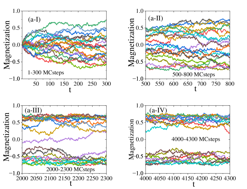
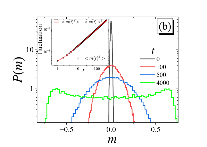
Figure 1: (a) Aging in the time evolution of magnetization in the two-dimensional Ising model with Metropolis dynamics for $L=100$, with time intervals $\Delta t=300$, and initial times $t_{0}=0$, $500,2000$ and $4000$. (b) Histograms of magnetization for different values of $t_{0}$, following a Gaussian distribution with variance defined by Equation 8. The Gaussian behavior is disrupted in the equilibrium state ($t_{0}\sim 4000$) when we observed that the system undergoes a slight transition into the ordered phase due to finite size scaling. The inset plot demonstrates that the difference $\left\langle m^{2}\right\rangle-\left\langle m\right\rangle^{2}$ exhibits the same power-law behavior as $\left\langle m^{2}\right\rangle$ in the short time regime, as $\left\langle m\right\rangle$ is approximately 0.

First, in Fig. 1 (a), we observe different evolutions of magnetization in the two-dimensional Ising model for various values of $t_{0}$, while keeping the observation time $\Delta t$ constant at 300.

We can observe histograms of magnetization for different values of $t_{0}$ in Fig. 1 (b), following a Gaussian distribution (Eq. 7) with variance defined by Eq. (8).

The Gaussian behavior is disrupted at equilibrium ($t_{0}\sim 4000$). The inset plot in the same figure demonstrates that $\left\langle m^{2}\right\rangle-\left\langle m\right\rangle^{2}$ and $\left\langle m^{2}\right\rangle$ exhibit the same power-law behavior, as $\left\langle m\right\rangle\approx 0$. Fitting Eq. (8) yields the well-known result from the literature: $\xi=0.801(1)$ for $\left\langle m^{2}\right\rangle$, which is in complete agreement with the expected value of $\xi=\frac{d}{z}-2\frac{\beta}{\nu z}\approx 0.802$, utilizing $z\approx 2.165$ from [10, 11], and $\frac{\beta}{\nu z}=0.0606$ from [7]. This agreement holds true even without starting from initial configurations with $m_{0}=0$, as is traditionally done in computer simulations within the context of short-time dynamics. Additionally, we obtained $A=0.00026(3)$.

From a simulation standpoint, the idea is to interrupt the simulation while preserving the configuration at time $t_{0}$. This configuration is then used as the initial state to calculate the correlation $C(t,t_{0})$. The first crucial aspect is to determine if there is a finite time scaling for $C(t,t_{0})$ as predicted by $A(t,t_{0})$.

In other words, for very large $t_{0}$, $C(t,t_{0})$ does not depend on $t_{0}$. However, according to scaling theory, for sufficiently large but not excessively large $t_{0}$, $C(t,t_{0})$ still exhibits a dependence on $t_{0}$.

In this paper, we aim to address this point and propose a conjecture regarding the aging time scaling law:

$$C(t,t_{0})=t_{0}^{\xi}g(\frac{t}{t_{0}}),$$ (9)

where $\xi=\frac{2-\eta}{z}$, and $g(x)\sim x^{\theta}$. Here, $\eta=\frac{2\beta}{\nu}$, and based on short-time theory, the exponent $\xi$ is precisely expected in the second moment of magnetization $\left\langle m^{2}\right\rangle\sim t^{\xi}$ when starting from random initial conditions with $m_{0}$ exactly equal to 0.

Building upon the methodology primarily developed by Henkel and Pleimling [3], and bolstered by valuable suggestions from anonymous referees of this work, we will demonstrate that this quantity serves as a correlator in momentum space and is expected to exhibit numerical scaling according to Eq. (9).

Utilizing the Ising model as a simplification, our objective is to numerically verify such scaling. We will demonstrate that considering the magnetization distribution from Eq. (7) to select spins is sufficient to reproduce $C(t,t_{0})$. However, we must also scale the time by $t_{0}$ to account for the effects of non-zero spatial correlations $\left\langle\sigma_{i}\sigma_{j}\right\rangle$.

Another important aspect addressed in this paper is the determination of the critical properties of the system when it is out of equilibrium. Specifically, we investigate the role of $t_{0}$ in determining the critical properties of the system.

To examine this, we explore the effects of $t_{0}$ on the short-time properties of the system using a recent method based on random matrices. We developed this method to determine criticality by analyzing spectral quantities obtained from Wishart-like matrices constructed from the time evolutions of magnetization. In this current manuscript we will demonstrate that the spectra is significantly influenced when large values of $t_{0}$ are used.

In the next subsection, we will provide a brief description of this method.

2.1 Criticality in nonequilibrium regime using Wishart-like matrices of magnetization

The signature of criticality out of equilibrium seems to be even more prominently manifested than what can be observed when uncorrelated systems ($T\rightarrow\infty$) are brought to finite temperatures, particularly around $T\approx T_{C}$.

In a recent study presented at [12], we examined the response of spectra in random matrices constructed from time evolutions of magnetization in earlier stages of a spin system. Our findings demonstrated the influence of criticality out of equilibrium on the spectral properties of statistical mechanics systems. We specifically utilized the short-range two-dimensional Ising model as a test model, as well as long-range mean-field systems [13].

To conduct such a test, we need to construct the magnetization matrix element $m_{ij}$, which represents the magnetization of the $j$-th time series at the $i$-th Monte Carlo step of a system with $N$ spins. Here, i ranges from 1 to $N_{MC}$, and $j$ ranges from $1$ to $N_{sample}$. Therefore, the magnetization matrix $M$ has dimensions $N_{MC}\times N_{sample}$. To analyze spectral properties, an interesting alternative is to consider not $M$, but the square matrix of size $N_{MC}\times N_{sample}$:

$$G=\frac{1}{N_{MC}}M^{T}M\ ,$$ (10)

where $G_{ij}=\frac{1}{N_{MC}}\sum_{k=1}^{N_{MC}}m_{ki}m_{kj}$, which is known as the Wishart matrix (see for example [14, 15, 16]). At this stage, instead of working with $m_{ij}$, it is more convenient to utilize the matrix $M^{\ast}$, defining its elements with the standard variables: $m_{ij}^{\ast}=(m_{ij}-\left\langle m_{j}\right\rangle)/\sqrt{\left\langle m_{j}^{2}\right\rangle-\left\langle m_{j}\right\rangle^{2}}$, where $\left\langle m_{j}^{k}\right\rangle=\frac{1}{N_{MC}}\sum_{i=1}^{N_{MC}}m_{ij}^{k}$.

Therefore, $G_{ij}^{\ast}=\frac{\left\langle m_{i}m_{j}\right\rangle-\left\langle m_{i}\right\rangle\left\langle m_{j}\right\rangle}{\sigma_{i}\sigma_{j}}$, where $\left\langle m_{i}m_{j}\right\rangle=\frac{1}{N_{MC}}\sum_{k=1}^{N_{MC}}m_{ki}m_{kj}$ and $\sigma_{i}=\sqrt{\left\langle m_{i}^{2}\right\rangle-\left\langle m_{i}\right\rangle^{2}}$. Analytically, if $m_{ij}^{\ast}$ are uncorrelated random variables, in this case, the density of eigenvalues $\sigma(\lambda)$ of the matrix $G^{\ast}$ follows the well-known Marcenko-Pastur distribution (see for example [17]) , which is expressed as:

$$\sigma(\lambda)=\left\{\begin{array}[]{l}\tfrac{N_{MC}}{2\pi N_{sample}}\tfrac{\sqrt{(\lambda-\lambda_{-})(\lambda_{+}-\lambda)}}{\lambda}\ ~{}~{}\text{if\ }~{}~{}~{}\lambda_{-}\leq\lambda\leq\lambda_{+}\\ \\ 0\ \ \ \text{otherwise}\end{array}\right.$$ (11)

where $\lambda_{\pm}=1+\frac{N_{sample}}{N_{MC}}\pm 2\sqrt{\frac{N_{sample}}{N_{MC}}}.$

However, for $T\neq T_{c}$, $\sigma(\lambda)$ does not follow the equation (11). The behavior of $\sigma(\lambda)$ obtained from MC time series simulated at different temperatures suggests a strong conjecture that the average eigenvalue $\left\langle\lambda\right\rangle=\int\nolimits_{0}^{\infty}\lambda\sigma(\lambda)d\lambda$ reaches a minimum at the critical temperature, while the variance $var(\lambda)=\left\langle\lambda^{2}\right\rangle-\left\langle\lambda\right\rangle^{2}$ exhibits an inflection point at the same critical temperature, where $\left\langle\lambda^{2}\right\rangle=\int\nolimits_{0}^{\infty}\lambda^{2}\sigma(\lambda)d\lambda$. Alternatively, a more precise identification can be made using the negative of the derivative of the variance:

$$c=-\frac{\partial var(\lambda)}{\partial T}$$ (12)

This behavior is also observed in the Potts model [18]. Therefore, the idea here is to observe if such fluctuations behave differently when we vary the starting index $i$ from $t_{0}$ to $t=t_{0}+\Delta t$, while keeping $\Delta t=N_{MC}$ fixed.

3 Results

Our results are structured into two distinct sections. In the first section, we provide a comprehensive justification for the scaling of Eq. (9), employing a rigorous methodology rooted in Fourier space studies. This approach builds upon the foundational work of Henkel and Pleimling [3], which we have extended to accommodate Fourier space investigations. In the second section, we present the numerical evidence substantiating this scaling behavior.

3.1 Correlator in Fourier space

The two-time correlation function can be formally defined as:

$$C(t,t_{0};\vec{r})=\left\langle m(t,\vec{r})m(t_{0},\vec{0})\right\rangle-\left\langle m(t,\vec{r})\ \right\rangle\left\langle m(t_{0},\vec{0})\right\rangle$$ (13)

where $m(t,\vec{r})$ is the order-parameter at time $t$ and position $r$, and $C(t,t_{0};\vec{r})=\left\langle m(t,\vec{r})m(t_{0},\vec{0})\right\rangle$ for fully disordered initial state $\left\langle m(t,\vec{r})\right\rangle=\left\langle m(t,\vec{0})\right\rangle=0$.

Given the assumption of spatial translation invariance, it follows that the two-time temporal-spatial spin-spin correlator must adhere to the following equation:

$$C(t,t_{0};\vec{r})=\kappa^{\phi}C(\kappa^{z}t,\kappa^{z}t_{0};\kappa\vec{r})\text{,}$$ (14)

where $\kappa$ is a rescaling factor, while $\phi$ is an exponent that can be determined by performing the scaling operation: $\kappa=\frac{1}{t_{0}^{1/z}}$. In this instance:

$$C(t,t_{0};\vec{r})=t_{0}^{-\phi/z}C(\frac{t}{t_{0}},1;\frac{\vec{r}}{t_{0}^{1/z}})$$ (15)

Thus, we write:

$$C(\frac{t}{t_{0}},1;\frac{\vec{r}}{t_{0}^{1/z}})=F_{C}(\frac{t}{t_{0}};\frac{\vec{r}}{t_{0}^{1/z}})$$ (16)

At criticality, in the equilibrium as t approaches infinity $(t\rightarrow\infty)$, we know that $C(t,t;\vec{r})$ must exhibit algebraic behavior as

$$C(t,t;\vec{r})\sim r^{-(d-2+\eta)}$$ (17)

where $\left|\vec{r}\right|$ represents the magnitude of $r$. By substituting $t=t_{0}$, we can observe that: $F_{C}(1;\frac{\vec{r}}{t^{1/z}})=F(\frac{r}{t^{1/z}})$. Using Eq. (15), we can express $C(t,t;\vec{r})$ as $t^{-\phi/z}F(\frac{r}{t^{1/z}})$. Comparing this with Eq. (17) yields: $F(\frac{r}{t^{1/z}})\sim\left(\frac{r}{t^{\frac{1}{z}}}\right)^{-\phi}$, where $\phi=d-2+\eta$. Returning to Eq. (15), we find:

$$C(t,t_{0};\vec{r})=t_{0}^{-(d-2+\eta)/z}F_{C}(\frac{t}{t_{0}};\frac{\vec{r}}{t_{0}^{1/z}})$$ (18)

Dynamical symmetry arguments, however, suggest that for $t\gg t_{0}$:

$$\begin{array}[]{lll}F_{C}(\frac{t}{t_{0}};\frac{\vec{r}}{t_{0}^{1/z}})&=&\left(\frac{t}{t_{0}}\right)^{-\frac{\lambda_{C}}{z}}F_{C}(1;\frac{\vec{r}}{t^{1/z}})\\ &&\\ &=&\left(\frac{t}{t_{0}}\right)^{-\frac{\lambda_{C}}{z}}\mathcal{F}(\frac{\vec{r}}{t^{1/z}})\\ &&\\ &=&\left(\frac{t}{t_{0}}\right)^{-\frac{\lambda_{C}}{z}}\mathcal{F}(\frac{t_{0}^{1/z}}{t^{1/z}}\frac{\vec{r}}{t_{0}^{1/z}})\end{array}$$ (19)

where $\lambda_{C}$ is an exponent similar to how $\phi$ was considered. Thus,

$$C(t,t_{0};\vec{r})=t_{0}^{-(d-2+\eta)/z}\left(\frac{t}{t_{0}}\right)^{-\frac{\lambda_{C}}{z}}\mathcal{F}(\frac{t_{0}^{1/z}}{t^{1/z}}\frac{\vec{r}}{t_{0}^{1/z}})$$ (20)

one has and when $r$ equals zero, one has

$$A(t,t_{0})=C(t,t_{0};0)=t_{0}^{-(d-2+\eta)/z}\mathcal{F}(0)\left(\frac{t}{t_{0}}\right)^{-\frac{\lambda_{C}}{z}}\sim\left(\frac{t}{t_{0}}\right)^{-\frac{\lambda_{C}}{z}}\text{,}$$ (21)

which leads to Eq. (2) in the limit of large times if $F(0)$ is a constant. It should also be noted that we introduced $\lambda_{C}$, the symbol for the autocorrelation exponent, with a purpose, and its value is determined by

$$\lambda_{C}=d-z\theta\text{,}$$ (22)

according to results obtained by Jansen, Schaub, and Schmittmann [1], where $\theta=(x_{0}-\frac{\beta}{\nu})/z$ represents the initial slip exponent. Here, $\beta$ and $\nu$ denote the static exponents, and $x_{0}$ is known as the anomalous dimension of magnetization [7]. For an interesting method to determine $x_{0}$, please refer to [19].

In addition, $\theta$ is precisely the same exponent as $C(t)$ in Eq. (4). It can take on positive values (see, for example, [6, 8, 7, 20]), negative values as observed in two-dimensional tricritical points [20, 21], or even very small values as seen in the 4-state Potts model due to the presence of a marginal operator [19].

By defining the spatial Fourier transform of $C(t,t_{0};\vec{r})$ as:

$$\widehat{C}(t,t_{0};\vec{p})=\int_{\mathbb{R}^{d}}d^{d}\vec{r}\ e^{i\vec{p}\cdot\vec{r}}C(t,t_{0};\vec{r})$$ (23)

where $d^{d}\vec{r}=dx_{1}dx_{2}...dx_{d},$one has:

$$\begin{array}[]{lll}\widehat{C}(t,t_{0};\vec{0})&=&\int_{\mathbb{R}^{d}}d^{d}\vec{r}\ C(t,t_{0};\vec{r})\\ &&\\ &=&t_{0}^{-(d-2+\eta)/z}\left(\frac{t}{t_{0}}\right)^{-\frac{\lambda_{C}}{z}}\int_{\mathbb{R}^{d}}\mathcal{F}(\frac{\vec{r}}{t^{1/z}})d^{d}\vec{r}\\ &&\\ &=&t_{0}^{-(d-2+\eta)/z}\left(\frac{t}{t_{0}}\right)^{-\frac{\lambda_{C}}{z}}t^{d/z}\int_{\mathbb{R}^{d}}\mathcal{F}(\vec{u})d^{d}\vec{u}=C\ t_{0}^{\frac{(2-\eta)}{z}}\left(\frac{t}{t_{0}}\right)^{\theta}\end{array}$$ (24)

where $C=\int_{\mathbb{R}^{d}}F(\vec{u})d^{d}\vec{u}$ is supposedly a constant. Thus, by utilizing the relation from Eq. (22) and denoting our original $C(t,t_{0})$ as $\widehat{C}(t,t_{0};\vec{0})$, one obtains:

$$C(t,t_{0})\sim t_{0}^{\frac{(2-\eta)}{z}}\left(\frac{t}{t_{0}}\right)^{\theta}\text{,}$$ (25)

by confirming the behavior described in Eq. (9) for $t\gg t_{0}$. Pleimling and Gambassi [22] as well as Henkel et al. [23] have investigated numerical results related to aging in the Fourier space of response functions, although they did not focus on correlation as we do in this current study.

With these results in hand, we can now delve into numerical findings regarding this scaling and other aging effects

3.2 Numerical Studies

We performed two-dimensional Monte Carlo (MC) simulations on the Ising model in two dimensions, precisely at the critical temperature denoted as $T=T_{C}=\frac{2}{\ln(1+\sqrt{2})}$, employing the Metropolis dynamics with single-flip spins.

We vary $t_{0}$. In all numerical experiments of this study, we used $L=128$. By starting from random initial configurations with $\left\langle m_{0}\right\rangle=0$, we calculated $C(t,t_{0})$ considering averages over $N_{run}=40000$ different runs. We explored different values of $t_{0}$. The initial question to address is determining the optimal value of $\tau$ for which the quantity $C(t,t_{0})$ $\times$ $(t-t_{0}+\tau)$ follows a power law. Is $\tau$ approximately equal to $t_{0}$?

Thus, in order to check if $\tau$ $\approx t_{0}$, for each $t_{0}$, we vary $\tau$ and examine the behavior of $C(t,t_{0})$ as a function of $t-t_{0}+\tau$ in a log-log scale for different values of $\tau$. Figure 2 (a) depicts the case where $t_{0}=100$.

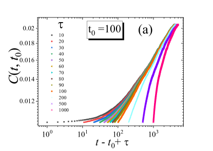
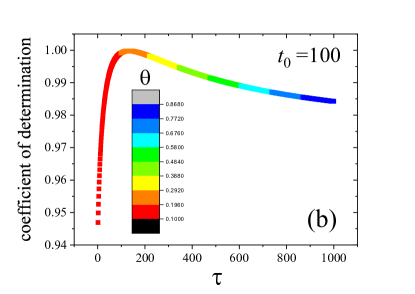
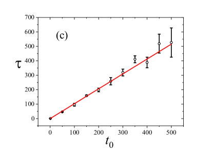
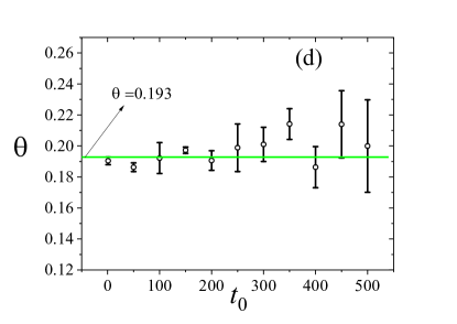
Figure 2: (a) $C(t_{0},t)$ as a function of $t-t_{0}+\tau$ for the case $t_{0}=100$, with varying values of $\tau$. We can observe that the power law behavior occurs when $\tau\approx t_{0}=100$. (b) Coefficient of determination for the fitting with different values of $\tau$. The maximum value occurs when $\tau\approx t_{0}=100$. The values of $\theta$ are represented in different colors according to the legend’s gradient. The optimal situation (peak values) includes $\theta\approx 0.19$, as expected. (c) Optimal value of $\tau$ as a function of $t_{0}$. (d) Corresponding value of $\theta$ for the optimal $\tau$ at each $t_{0}$.

The power-law behavior becomes evident (qualitatively) when $\tau$ is approximately equal to $t_{0}$, which in this case is 100. The $\theta$ values are visually represented using various colors to denote different gradients, as specified in the legend. These values are derived by conducting linear fits of $\ln C(t_{0},t)\times\ln(t-t_{0}+\tau)$ for each $\tau$ as depicted in Fig. 2 (b).

This observation is reinforced by the fact that the maximum coefficient of determination, which approaches 1, is achieved when $\tau$ is approximately equal to $t_{0}$ (100). This coefficient serves as a robust indicator of the fitting quality, with values closer to 1 signifying a superior fit. Its utility in the field of Statistical Mechanics has been extensively explored for the determination of critical parameters (for further reference, please consult [24]).

The region of the optimal fit reveals a $\theta$ value close to the expected $0.19$. In Figure 2 (c), we depict the linear trend of the optimal $\tau$ value, which corresponds to the highest coefficient of determination, in relation to $t_{0}$. The linear regression analysis produces $\tau=b$ $t_{0}$, with $b=1.03\pm 0.02$, providing additional evidence that $\tau$ remains approximately equal to $t_{0}$ regardless of the specific $t_{0}$ value. These error bars are calculated based on data from five different seed values.

Lastly, Figure 2 (d) presents the corresponding $\theta$ values corresponding to the optimal $\tau$ values determined for various $t_{0}$ values.

The green line corresponds to the value observed in short-time simulations from Ising-like models (in the same universality class) mentioned in various references (see, for example: [6, 7, 8, 20]).

We now test the scaling relation given by Equation (9). To do so, we consider the correlation divided by the initial second moment:

$$C^{\ast}(t,t_{0})=\frac{\left\langle m(t)m(t_{0})\right\rangle}{\left\langle m(t_{0})^{2}\right\rangle}$$ (26)

as function of $t$, $t-t_{0}$, and finally $t/t_{0}$, presented in three different plots, all of them using log-log scale for the quantities, here indexed by (a), (b), and (c) respectively in Fig. 3. Fig. 3 (c) suggests that scaling described by Eq: (9).

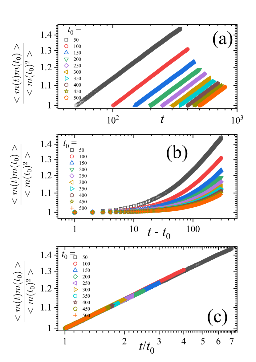
Figure 3: Plots of the correlation divided by the initial second moment are shown as functions of $t$ (a), $t-t_{0}$ (b), and $t/t_{0}$. An excellent scaling is observed in plot (c), as predicted by Eq: 9.

These plots nicely illustrate the three defining criteria of aging [3]: (a) slow dynamics, (b) breaking of time-translation invariance and (c) dynamical scaling with its characteristic data collapse.

This scaling is performed using the quantity $\left\langle m(t_{0})^{2}\right\rangle$ (or $\left\langle m(t_{0})^{2}\right\rangle-\left\langle m(t_{0})\right\rangle^{2}$ since $\left\langle m(t_{0})\right\rangle=0$). Alternatively, we can perform the scaling according to Eq. (9) by dividing $C(t,t_{0})$ by $t_{0}^{b}$ while adjusting the value of $\xi$ to optimize the scaling. We also conducted a test to verify this, and the results are presented in Fig. 4. We found that $b=0.806$ is the optimal value that matches Eq. (9), which is very similar to $\xi=0.8010(4)$, the expected exponent for the time evolution of $\left\langle m^{2}(t)\right\rangle$, by demonstrating that the definition of $C^{\ast}(t,t_{0})$ as outlined in Eq. (26) aligns seamlessly with the concepts presented in the developments explored within subsection 3.1.

Figure 4: Direct scaling by fitting $b$ that better corresponds to Eq. 9. We find $b=0.806$, which is very similar to $\xi=0.8010(4)$, expected to be the exponent of the time evolution of $\left\langle m^{2}(t)\right\rangle$.

Since the magnetization distribution at an arbitrary time $t_{0}$ follows Eq. (7), the question is whether considering an initial condition with magnetization distributed accordingly would yield the same correlation $C(t,t_{0})$ as calculating it with the initial condition that the system obtained at that time. In other words, does the obtained $C(t,t_{0})$ remain the same?

To explore this, we prepared systems with the initial condition described by Eq. (7) using many different samples with different $m_{0}$ values, but with the condition $\left\langle m_{0}^{2}\right\rangle=At_{0}^{\xi}$. We chose $t_{0}$ values of $50,100,200$, and $300$, which resulted in $\sqrt{\left\langle m_{0}^{2}\right\rangle}=A^{1/2}t_{0}^{\xi/2}=0.077$, $0.102$, $0.135$, and $\allowbreak 0.158$, respectively.

So, using these standard deviations, we generate $m_{0}$ according to Eq. (7), and the spins are randomly chosen with the probability: $p(\sigma_{i})=\frac{1+m_{0}\sigma_{i}}{2}$, where $\sigma_{i}=1,...,N$. It is important to note that $p_{-}+p_{+}=1$. We then evolve the system and compare $C(t,t_{0})$ with the results obtained by preparing the initial condition according to a Gaussian distribution with the predicted variance previously established. Figure 5 illustrates this comparison.

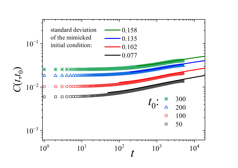
Figure 5: Verification of $C(t,t_{0})$ for different values of $t_{0}$ (points) versus correlation by mimicking the initial distribution of spins (continuous curves). We have scaled the time for the simulations with mimicked initial condition by multiplying $t$ by $t_{0}$.

It is essential to mention that we had to scale the time by multiplying $t$ by $t_{0}$ in the case of evolutions with mimicked initial conditions. It is interesting because it suggests that the spatial correlation of spins has an important role, and its effects determine the time scaling of the system and not only the distribution of magnetization to be a Gaussian according to Eq. (7). However, we can observe that curve for $C(t,t_{0})$ can be reproduced if we suitably scale the time.

3.3 Aging and random matrices

Finally, we test the effects of aging on the spectral method sensitive to determine the critical properties of the system. So we build matrices for $N_{sample}=100$, considering $\Delta t=N_{MC}=300$, and considering different values of $t_{0}$. The result is interesting because for $t_{0}=50$, for example, we observe a minimum of eigenvalue mean at $T=T_{C}$ in previous works, however when the aging is more significant, we observe a visible deviation of such minimum as suggested by Fig. 6 (a).

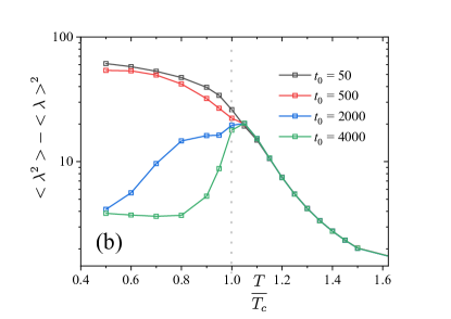
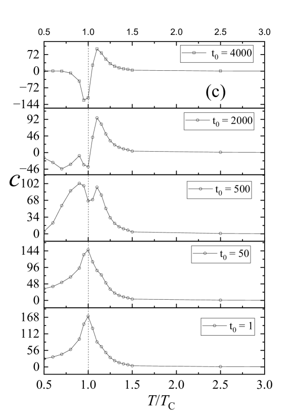
Figure 6: (a) Eigenvalue average as a function of $T/T_{C}$. A deviation from the minimum at $T=T_{c}$ is found for $t_{0}>50$, as can be observed. (b) The variance of eigenvalues for different temperatures and (c) The negative derivative of this same variance.

A deviation from the minimum at $T=T_{c}$ is found for $t_{0}>50$, as can be observed. Thus it is interesting the sensitivity of spectra considering time series with aging. The same can be observed on the other spectral parameters such as the variance of eigenvalues for different temperatures Fig. 6 (b), and Fig. 6 (c), that shows the pronounced peak on the negative of the derivative of this same variance when no aging is considered. However, after the peak ($t_{0}=1$), we observe a double peak ($t_{0}=500$) and subsequent discontinuity in the vicinity of $T/T_{C}=1$, and there is no consensus regarding the localization of the critical parameter. This lack of consensus is particularly pronounced for $t_{0}>50$, where finite-size effects appear to be significant and influence the localization.

4 Conclusions

We conducted a study on aging phenomena by examining the scaling behavior of the total correlation of magnetization. Such scaling is corroborated by an analysis of the correlator in Fourier space according to methodology developed by Henkel and Pleimling [3]. Our findings reveal an important deviation in the scaling of the second moment of magnetization. Moreover, we demonstrate that when considering the initial magnetization distributed according to the Gaussian distribution expected at the time we hypothetically started after interrupting the time-dependent simulations, we need to scale the time appropriately to capture the correlation obtained with this initial time.

Furthermore, we present an intriguing analysis of random matrices, which sheds light on the expected spectra of matrices constructed from the time evolutions of magnetization during aging. This method exhibits high sensitivity and demonstrates how aging can impact the determination of the critical temperature under the influence of finite size scaling effects.

Overall, our study provides valuable insights into the effects of aging on magnetization dynamics and highlights the importance of accounting for initial conditions and scaling considerations in such systems. It is important to stress, that Pleimnling and Gambassi, and Henkel et. al much before had obtained other numerical examples for studies in Fourier space however by concerning response functions [22, 23].

Lastly, it is crucial to note that the irrelveant of $t_{0}$ in the renormalization-group sense was previously established at $T=T_{C}$ by Calabrese and Gambasi [25]. They conducted a meticulous comparison of correlators and responses in both direct and momentum space. Our results align with their findings, as our short-ranged initial correlation, in theory, should not alter the critical exponents.

It is also important to note that for temperatures below the critical point ($T<T_{C}$), Janke and colleagues [9], have established that scaling laws, which remain invariant regardless of the selection of $t_{0}$, are likely associated with the behavior $\left\langle m(t)^{2}\right\rangle\sim t^{d/z}$, even in the context of long-range systems.

CRediT authorship contribution statement

All authors conceived and designed the analysis, performed formal analysis, wrote the paper, elaborated the algorithms, analysed the results, and reviewed the manuscript.

Declaration of competing interest

The authors declare that they have no known competing financial interests or personal relationships that could have appeared to influence the work reported in this paper

Funding

R. da Silva would like to thank CNPq for financial support under grant number 304575/2022-4.

References

- [1] H. K. Janssen, B. Schaub, B. Schmittmann, Z. Phys. B: Condens. Matter 73, 539 (1989)
- [2] D. A. Huse. Phys. Rev. B 40, 304 (1989)
- [3] M. Henkel, M. Pleimling, Non-equilibrium Phase Transitions, Vol. 2: Ageing and Dynamical Scaling far from Equilibrium, Springer, Dordrecht (2010) , M. Henkel Cond. Matt. Phys. 26, 13501 (2023), https://doi.org/10.48550/arXiv.2211.03657
- [4] M. Hase, T. Tome, M. J. de Oliveira, Phys. Rev. E 82, 011133 (2010)
- [5] W. Liu, U. C. Tauber, EPL 128, 30006 (2019), https://doi.org/10.48550/arXiv.1910.01168
- [6] T. Tome, M. J. de Oliveira, Phys. Rev. E 58, 4242 (1998)
- [7] B. Zheng, Int. J. Mod. Phys. B 12, 1419 (1998)
- [8] E. V. Albano, M. A. Bab, G. Baglietto, R. A. Borzi, T. S. Grigera, E. S. Loscar, D. E. Rodriguez, M. L. R. Puzzo, G. P. Saracco, Rep. Prog. Phys. 74, 026501 (2011)
- [9] W. Janke, H. Christiansen, S. Majunder, Eur. Phys. J. Spec. Top 232, 1693–1701 (2023)
- [10] M. P. Nightingale, H. W. Blote, Phys. Rev. Lett. 76, 4548 (1996)
- [11] N. Ito, Physica A 196, 591 (1993)
- [12] R. da Silva, Int. J. Mod. Phys. C 34, 2350061 (2023), https://doi.org/10.48550/arXiv.2206.01035
- [13] R. da Silva, H. C. Fernandes, E. Venites Filho, S. D. Prado, J. R. Drugowich de Felicio, Braz. J. Phys. 53, 80 (2023), https://doi.org/10.48550/arXiv.2303.02003
- [14] J. Wishart, Biometrika 20A, 32 (1928)
- [15] Vinayak, T. H. Seligman, AIP Conf. Proc. 1575, 196 (2014)
- [16] C. Recher, M. Kieburg, T. Guhr, Phys. Rev. Lett. 105, 244101 (2010), https://doi.org/10.48550/arXiv.1006.0812, T. Wirtz, T. Guhr, Phys. Rev. Lett. 111, 094101 (2013), https://doi.org/10.48550/arXiv.1306.4790
- [17] A.M. Sengupta, P.P. Mitra, Phys. Rev. E 60, 3389 (1999)
- [18] R. da Silva, E. Venites, S. D. Prado, J. R. Drugowich de Felicio, https://doi.org/10.48550/arXiv.2302.07990 (2023)
- [19] R. da Silva, J. R. Drugowich de Felício, Phys. Lett. A 333, 277 (2004), https://doi.org/10.48550/arXiv.cond-mat/0404083
- [20] R. da Silva, N. A. Alves, and J. R. Drugowich de Felicio, Phys. Rev. E 66, 026130 (2002), https://doi.org/10.48550/arXiv.cond-mat/0204346
- [21] R. da Silva, H. A. Fernandes, J. R. Drugowich de Felício, W. Figueiredo, Comp. Phys. Comm. 184, 2371 (2013), https://doi.org/10.48550/arXiv.1511.06377
- [22] M. Pleimling, A. Gambassi, Phys. Rev. B 71, 180401(R) (2005), https://doi.org/10.48550/arXiv.cond-mat/0501483
- [23] M. Henkel, T. Enss, M. Pleimling, J. Phys. A 39, L589–L598 (2006), https://doi.org/10.48550/arXiv.cond-mat/0605211
- [24] R. da Silva, J. R. Drugowich de Felício, A. S. Martinez, Phys. Rev. E 85 066707 (2012), https://doi.org/10.48550/arXiv.1205.6789, R. da Silva, Phys. Rev. E 105 034114 (2022), https://doi.org/10.48550/arXiv.2110.15868
- [25] P. Calabrese, A. Gambassi, J. Phys. A 38, R133 (2005), https://doi.org/10.48550/arXiv.cond-mat/0410357