Scratch Team of Single-Rotor Robots and Decentralized Cooperative Transportation with Robot Failure

Abstract

Achieving cooperative transportation by teams of aerial robots has been attracting attention owing to its flexibility with respect to payloads and robustness against failures. In this paper, we propose a flexible decentralized controller for the number of robots and the shapes of payloads in a cooperative transport task using multiple single-rotor robots. Our controller is robust to mass and center of mass fluctuations and robot failures. Moreover, asymptotic stability against dynamics errors is guaranteed. Additionally, the controller supports heterogeneous single-rotor robots. Thus, robots with different specifications and deterioration can be effectively utilized for cooperative transportation. In particular, this performance is effective for robot reuse. To achieve the aforementioned performance, the controller consists of a parallel structure comprising two controllers: a feedback controller, which renders the system strictly positive real, and nonlinear controller, which renders the object asymptotic to the target. First, we confirm cooperative transportation using 8 and 10 robots for two shapes via numerical simulation. Subsequently, the cooperative transportation of a rectangle payload (with a weight of approximately 3 kg and maximum length of 1.6 m) is demonstrated using a robot team consisting of three types of robots, even under robot failure and center of mass fluctuation.

Keywords Unmanned aerial vehicle  $\cdot$ Multi-agent systems  $\cdot$ Decentralized control

1 Introduction

Recently, with the advancement of aerial robots, the number of studies on aerial transportation and manipulation has significantly increased [1, 15, 27, 9, 12]. The demand for aerial transportation tasks has increased significantly, especially because of the impact of COVID-19 [14, 44, 34]. Cooperative transportation using multiple aerial robots has attracted attention as it can provide redundancy and scalability of the system for transporting various types of payloads [22, 11, 20, 6, 41]. Notably, the center-of-mass (COM) and mass of the payload should comply with the specifications of the aircraft when using a single aerial robot for transportation. Cooperative transportation using multiple aerial robots is scalable with respect to the mass of the payload, as long as the required number of robots can be added at the necessary positions without interference. Notably, redundant cooperative transportation becomes a robust system because, in an event of a single robot failure, other robots can compensate for the thrust. Furthermore, the practicality of the system improves because robots can easily be plugged in/plugged out if each robot can be controlled through a decentralized method [36, 37].

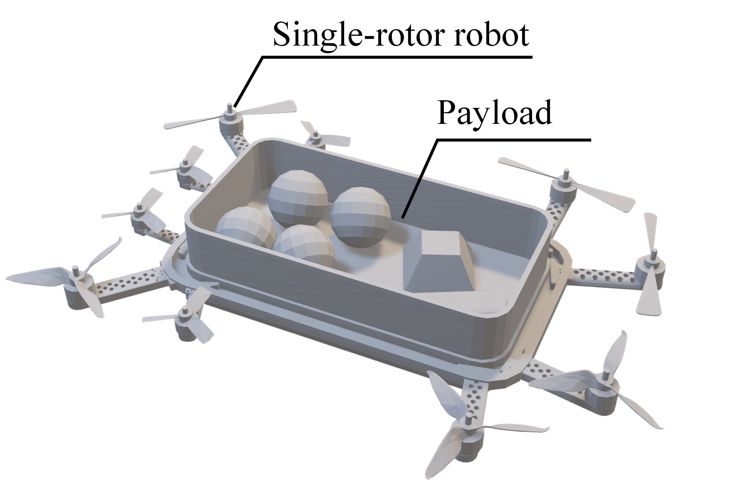
(a) Heterogenous configuration

(b) Real flight with decentralized controller with various disturbances

Figure 1: Consept

To adapt multi-robot systems to the real world, the configuration of the robot team should be expanded to include heterogeneous robots [8, 33, 5]. Studies on heterogeneous robots involve decomposing the overall task and assigning robots designed for different purposes [18, 35, 31], as well as achieving robots that perform the same task [30, 17, 45]. Tasks such as carrying a big desk in cooperation with people of various ages correspond to the situation of the same task. It is important for the robot team to be able to handle such tasks because robots with various performances are expected to appear in the future. In this study, we address performing such the transportation tasks with heterogeneous aerial robots. A possible scenario is a transportation task using a robot team of different manufacturers or a team of reuse robots. If such integration is achieved, aerial cooperative transportation would be practical in the field of robotics.

Considering a cooperative transportation system where a team of multi-copters is rigidly connected to the payload, each multi-copter can be viewed as a robot that applies force in the vertical and one rotational direction. Therefore, our previous study proposed a cooperative transportation model using a “single-rotor robot” to simplify the problem and production [26, 25]. Moreover, we achieved aerial cooperative transportation in an environment where an imbalance in the COM or robot failure occurs, using the proposed team of robots. Compared with the case in the previous study, in this study, the control target is changed to a heterogeneous team of robots, as shown in Fig. 1(a). The controller requires a high response because of different thrust characteristics of robots in the case of a heterogeneous team. For example, other robots need to promptly increase their thrust to compensate if a certain robot reaches its thrust limit due to low performance. Therefore, we propose a decentralized non-linear controller approach that switches to high gains based on the situation. Additionally, we prove the asymptotic stability of this controller. Furthermore, numerical simulations and experiments using an actual prototype are conducted. The contributions of this study are as follows:

• Proposal of a variable-gain decentralized controller with proven asymptotic stability for an aerial cooperative transportation using a heterogeneous team of robots

• Confirmation of the performance by two simulations with different numbers of robots and different shapes of payload

• Confirmation by an experiment using a real prototype with three different types of single-rotor robots under COM fluctuation and robot failure (Fig.1(b))

The remainder of this paper proceeds as follows. Section 2 describes related work of our proposal; Section 3 describes the model of the target system; Section 4 describes our controller; Section 5 describes the numerical experiments; Section 6 describes the results of prototype experiments; and Section 7 presents the advantage of our method and discusses the results of experiments. Finally, conclusions are presented in Section 8.

2 Related work

Cooperative transportation using aerial robots includes those using cables [22, 11, 42, 38] and those using rigid connections [20, 7, 43, 26, 25]. Rigid configurations are better suited to take advantage of the fault-robustness than cables. It is because the robot failures of the cabled configurations result in not only a loss of thrust but also in a reduction in the impact of the aerial robots. In addition, Oung et al. [28] and Mu et al. [24] modularized their robots to improve scalability. We noted these advantages and address control of a team of single-rotor robots rigidly connected to the payload.

Previous studies have focused on the control of aerial cooperative transportation that can be categorized into centralized and decentralized approaches. In centralized control, Wang [42] proposed a centralized robust controller based linear quadratic gaussian. This controller is robust against mass fluctuations of about 20 % in aerial cooperative transportation using cables. Moreover, Pereria et al. [30, 29] realized the aerial transportation of a round bar object by two different types of robots. This controller which was based on proportional—integral–derivative (PID) using ideal control input guaranteed stability. Furthermore, Mu et al. [24] proposed an adaptive controller which utilizes estimated states using the inertial measurement unit (IMU) mounted on each robot. This controller allows for stable flight in various configurations. The centralized control in aerial transportation requires equipment and infrastructure to share information because it utilizes all available data. Realizing stable flight by distributed control can reduce the need for extensive information sharing and relax the constraints of this equipment.

The decentralized controller with a basic aerial cooperative transportation model of rigid configuration was proposed by Millinger et al. [20]. To achieve decentralized control, they assume that the positions of each robot are known. Wang et al. [43] and Shirani et al. [38] proposed decentralized control using the symmetrical arrangement of robot positions. Wang et al. used symmetry to relax the constraints on the robot’s position and used a wrench-based compensator to guarantee stability. Shirani et al. used feedback linearization and linear matrix inequality (LMI) to ensure stability. Cardona [4] utilized leader–follower controller to achieve decentralized control of heterogeneous robots for aerial cooperative transportation. Additionally, robustness against fluctuations in the reference was demonstrated. Furthermore, in our previous study [25], we proposed a decentralized controller that is robust against disturbances for aerial cooperative transportation using identical single-rotor robot and a switching controller [2]. An advantage of decentralized control in the field of robotics is often mentioned as being robust against robot failures [32, 13, 8]. However, this advantage has not received much attention in aerial cooperative transportation. Furthermore, to our best knowledge, there have been no studies that specifically focus on heterogeneous robots and their robustness in aerial cooperative transportation involving rigid connections.

In this study, we focused on decentralized cooperative control of heterogeneous multiple single-rotor robots in a real flight environment that includes mass and COM fluctuations as well as robot failure.

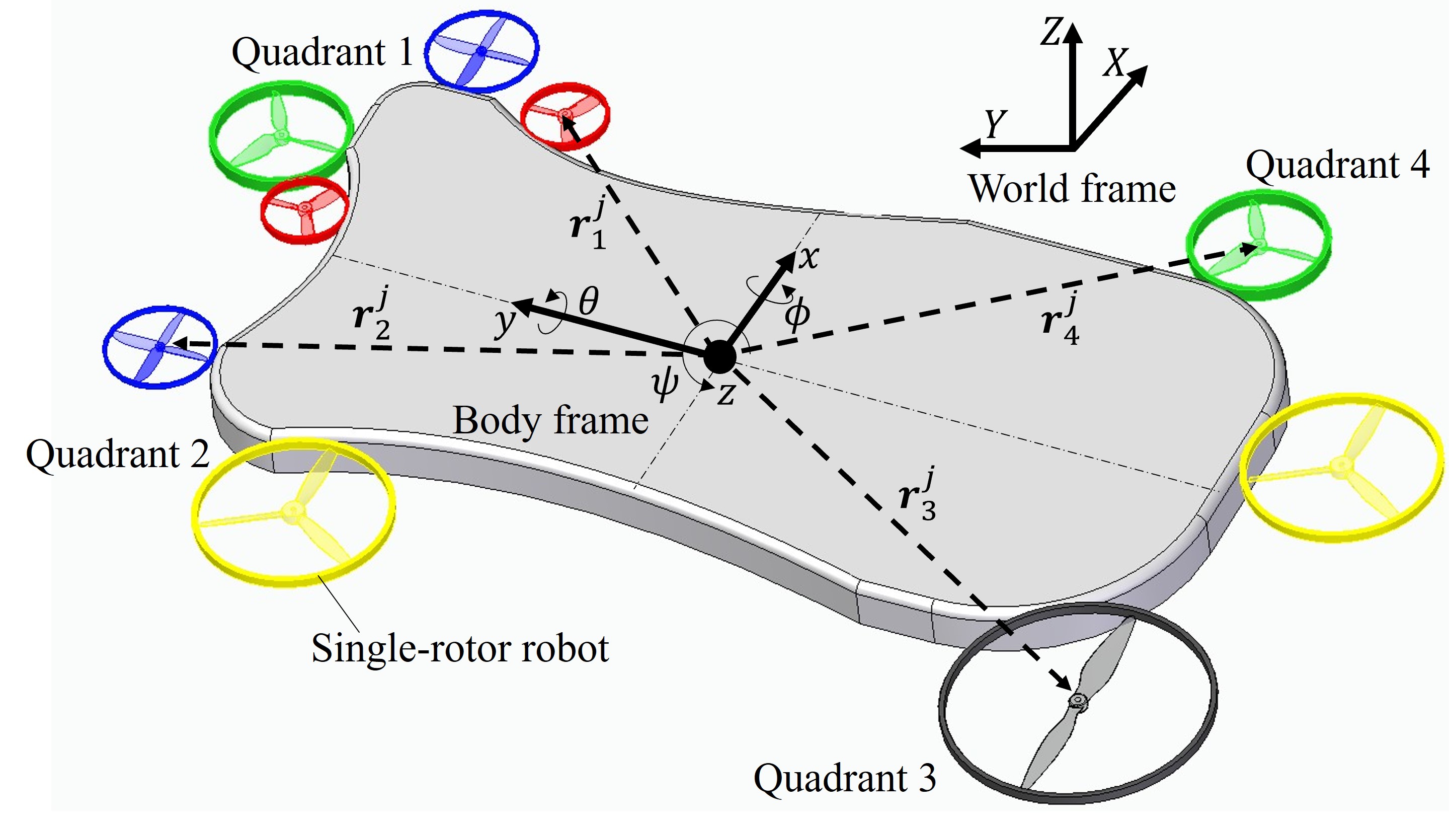
Figure 2: Model of cooperative transportation using heterogeneous single-rotor robots ($n_{1}=4$, $n_{2}=2$, $n_{3}=1$, $n_{2}=2$)

3 Modeling

We modeled the dynamics of cooperative transportation using heterogeneous single-rotor robots while focusing on the behavior of the force acting in each quadrant, as shown in Fig. 2. Let $n_{i}(i=1,\dots,4)$ be the number of robots in each quadrant; the dynamics of the hovering state can be approximated as follows [20]:

$$\begin{split}&m\left[\begin{array}[]{c}\ddot{x}\\ \ddot{y}\\ \ddot{z}\\ \end{array}\right]=\left[\begin{array}[]{c}mg\theta\\ -mg\phi\\ 0\\ \end{array}\right]+\left[\begin{array}[]{c}0\\ 0\\ \sum_{i=1}^{4}\sum_{j=1}^{n_{i}}u_{i}^{j}\\ \end{array}\right]-\left[\begin{array}[]{c}0\\ 0\\ mg\\ \end{array}\right]\\ &\bm{J}\left[\begin{array}[]{c}\ddot{\phi}\\ \ddot{\theta}\\ \ddot{\psi}\\ \end{array}\right]=\left[\begin{array}[]{c}\sum_{i=1}^{4}\sum_{i=1}^{n_{i}}\left(\bm{r_{i}^{j}}\times\bm{e_{3}}\right)_{12}u_{i}^{j}\\[7.0pt] \sum_{i=1}^{4}\sum_{j=1}^{n_{i}}d_{i}^{j}c_{qi}^{j}u_{i}^{j}\\ \end{array}\right],\end{split}$$ (1)

where $x$, $y$, and $z$ are the three-dimensional positions of the payload on a body frame system; $\phi$, $\theta$, and $\psi$ denote the roll, pitch, and yaw angles of the payload, respectively; $u_{i}^{j}$ denotes the thrust of the robot $j$ in quadrant $i$; $m$ and $\bm{J}$ denote the overall mass and moment of inertia, respectively; $\bm{r_{i}^{j}}\in\mathbb{R}^{3}$ denote the vector from the origin of the body frame system, the COM position of the payload, to the attachment position of the robot $j$ in quadrant $i$; $\bm{e_{3}}=[0,0,1]^{\top}$ denotes the unit vector of the $z$ axis; and $d_{i}^{j}\in\{1,-1\}$ denotes the rotational direction of the robot $j$ in quadrant $i$. Further, $c_{qi}^{j}$ denotes the thrust torque conversion coefficient of the robot $j$ in quadrant $i$, and $g$ denotes the gravitational acceleration. Note that the Coriolis force is assumed to be zero because $\dot{\phi}\simeq 0$ and $\dot{\theta}\simeq 0$ are assumed during hovering. A state expression of eq. (1) can be represented as follows:

$$\begin{split}\left[\begin{array}[]{c}\bm{\dot{x}}\\ \bm{\ddot{x}}\\ \bm{\dot{\phi}}\\ \bm{\ddot{\phi}}\\ \end{array}\right]&=\left[\begin{array}[]{cccc}\bm{0_{3}}&\bm{I_{3}}&\bm{0_{3}}&\bm{0_{3}}\\ \bm{0_{3}}&\bm{0_{3}}&\bm{G_{M}}&\bm{0_{3}}\\ \bm{0_{3}}&\bm{0_{3}}&\bm{0_{3}}&\bm{I_{3}}\\ \bm{0_{3}}&\bm{0_{3}}&\bm{0_{3}}&\bm{0_{3}}\\ \end{array}\right]\left[\begin{array}[]{c}\bm{x}\\ \bm{\dot{x}}\\ \bm{\phi}\\ \bm{\dot{\phi}}\\ \end{array}\right]\\ &+\left[\begin{array}[]{c}\bm{0_{3}}\\ \bm{B_{\bm{x}n}}\\ \bm{0_{3}}\\ \bm{B_{\bm{\phi}n}}\\ \end{array}\right]\bm{u_{n}}-\left[\begin{array}[]{c}\bm{0_{3\times 1}}\\ \bm{g_{V}}\\ \bm{0_{3\times 1}}\\ \bm{0_{3\times 1}}\\ \end{array}\right],\end{split}$$ (2)

where $\bm{x}=[x,y,z]^{\top}$, $\bm{\phi}=[\phi,\theta,\psi]^{\top}$ denotes the state, $\bm{u_{n}}=[u^{1}_{1},\dots,u_{4}^{n_{4}}]^{\top}\in\mathbb{R}^{n\times 1}$ denotes the control input, $\bm{g_{V}}=[0,0,g]^{\top}$ denotes the vector of the gravitational acceleration, $\bm{0_{i}}=\{0\}^{i\times i}$ denotes the zero matrix, $\bm{I_{j}}$ denotes a $j\times j$ identity matrix, and $\bm{0_{i\times j}}=\{0\}^{i\times j}$ denotes a zero matrix or zero vector. Moreover, $\bm{G_{M}}$, $\bm{B_{\bm{x}n}}$, and $\bm{B_{\bm{\phi}n}}$ are defined as

$$\begin{split}&\bm{G_{M}}=\left[\begin{array}[]{ccc}0&g&0\\ -g&0&0\\ 0&0&0\\ \end{array}\right]\\ &\bm{B_{\bm{x}n}}=\frac{1}{m}[\bm{e_{3}},\dots,\bm{e_{3}}]\in\mathbb{R}^{3\times n}\\ &\bm{B_{\bm{\phi}n}}=\bm{J}^{-1}\left[\begin{array}[]{ccc}\left(\bm{r_{1}^{1}}\times\bm{e_{3}}\right)_{12}&\dots&\left(\bm{r_{4}^{n_{4}}}\times\bm{e_{3}}\right)_{12}\\ d^{1}_{1}c^{1}_{q1}&\dots&d^{n_{4}}_{4}c^{n_{4}}_{q4}\\ \end{array}\right]\in\mathbb{R}^{3\times n}.\end{split}$$

Furthermore, $\ddot{x}\simeq g\phi$ and $\ddot{y}\simeq-g\theta$ are approximated because the focus herein is on the control in a state close to equilibrium. As equilibrium is assumed, the transforming coordinates from the body frame to world frame are given by

$$\left[\begin{array}[]{c}X\\ Y\\ Z\end{array}\right]=\left[\begin{array}[]{ccc}\cos{\psi}&-\sin{\psi}&0\\ \sin{\psi}&cos{\psi}&0\\ 0&0&1\end{array}\right]\left[\begin{array}[]{c}x\\ y\\ z\end{array}\right].$$

This study addressed fluctuations in mass and COM and robot failure. According to eq. (2), these fluctuations affect only the $\bm{B_{\bm{x}n}}$ and $\bm{B_{\bm{\phi}n}}$ matrices. Thus, we focused on the $\bm{B}$ matrix for control robustness.

4 Decentralized control

We propose a control approach that combines a variable gain version of an autonomous smooth switching controller (VG-ASSC) with a robust feedback controller (RFC) that ensures the strictly positive real (SPR) property of the system. The VG-ASSC is decentralized because it utilizes only broadcasted error. However, the target system must be SPR for the VG-ASSC to ensure asymptotic stability. By combining the VG-ASSC with the RFC, the stability and robustness of the overall control system can be improved. Therefore, the RFC changes the target system to an SPR system. Notably, this control maintains the equilibrium state. Therefore, in the proposed method, the references in the equilibrium state are gradually adjusted to approach a desired destination. This section first describes the RFC.

4.1 Strictly positive realization

First, we describe the transformation of the state model for strictly positive realization. Then, the RFC is introduced. In this section, we focus not only on the state equation but also on the output equation because the purpose of the RFC is to make system SPR.

4.1.1 Input transformation

Notably, the input matrix $[\bm{0}_{3},\bm{B_{\bm{x}n}},\bm{0}_{3},\bm{B_{\bm{\phi}n}}]^{\top}$ should be a full rank for the system to be SPR. Eq.(2) is converted to four inputs because the rank of the input matrix is four in the case of a flight system using rigidly connected rotors such as a multicopter. Therefore, we assumed the following:

• The robots located in each quadrant exist in the vicinity of the representative points located in each quadrant. Let $\bm{r_{i}}$ be the vector from the COM to the representative point in quadrant $i$; the vector of each robot in quadrant $i$ from the COM can be expressed as $\bm{r_{i}}$ ($\bm{r_{i}}\simeq\bm{r^{1}_{i}}\simeq\dots\simeq\bm{r_{i}^{n_{i}}}$).

• The directions of rotation of the rotor of the robots located in each quadrant are the same. Let $d_{i}$ be the rotation direction of the robots in quadrant $i$; the rotation direction of each robot in quadrant $i$ can be expressed as $d_{i}$ ($d_{i}=d_{i}^{1}=\dots=d_{i}^{n_{i}}$).

• The average thrust-torque coefficients of each quadrant are the same. Let $c_{q}$ be the average of the thrust-torque coefficient; the thrust-torque coefficient of each robot is $c_{q}$ ($c_{q}\simeq\frac{1}{n_{1}}\sum_{j=1}^{n_{1}}c_{q1}^{j}\simeq\dots\simeq\frac{1}{n_{4}}\sum_{j=1}^{n_{4}}c_{q4}^{j}$).

Under this assumption, eq. (2) can be transformed into a four-input equation as follows:

$$\begin{split}\left[\begin{array}[]{c}\bm{\dot{x}}\\ \bm{\ddot{x}}\\ \bm{\dot{\phi}}\\ \bm{\ddot{\phi}}\\ \end{array}\right]&=\left[\begin{array}[]{cccc}\bm{0_{3}}&\bm{I_{3}}&\bm{0_{3}}&\bm{0_{3}}\\ \bm{0_{3}}&\bm{0_{3}}&\bm{G_{M}}&\bm{0_{3}}\\ \bm{0_{3}}&\bm{0_{3}}&\bm{0_{3}}&\bm{I_{3}}\\ \bm{0_{3}}&\bm{0_{3}}&\bm{0_{3}}&\bm{0_{3}}\\ \end{array}\right]\left[\begin{array}[]{c}\bm{x}\\ \bm{\dot{x}}\\ \bm{\phi}\\ \bm{\dot{\phi}}\\ \end{array}\right]\\ &+\left[\begin{array}[]{c}\bm{0_{3\times 4}}\\ \bm{B_{X}}\\ \bm{0_{3\times 4}}\\ \bm{B_{\bm{\varPhi}}}\\ \end{array}\right]\bm{U}-\left[\begin{array}[]{c}\bm{0_{3\times 1}}\\ \bm{g_{V}}\\ \bm{0_{3\times 1}}\\ \bm{0_{3\times 1}}\\ \end{array}\right],\end{split}$$ (3)

where $\bm{U}=[U_{1},U_{2},U_{3},U_{4}]^{\top}(U_{i}=\sum_{j=1}^{n_{i}}u_{i}^{j})$ and $\bm{B_{X}}=\frac{1}{m}[\bm{e_{3}},\bm{e_{3}},\bm{e_{3}},\bm{e_{3}}]$. Moreover, $\bm{B_{\phi}}$ is expressed as follows:

$$\begin{split}&\bm{B_{\phi}}=\\ &\bm{J}^{-1}\left[\begin{array}[]{cccc}(\bm{r_{1}}\times\bm{e_{3}})_{12}&(\bm{r_{2}}\times\bm{e_{3}})_{12}&(\bm{r_{3}}\times\bm{e_{3}})_{12}&(\bm{r_{4}}\times\bm{e_{3}})_{12}\\ d_{1}c_{q}&d_{2}c_{q}&d_{3}c_{q}&d_{4}c_{q}\\ \end{array}\right].\end{split}$$

4.1.2 Error system

We convert eq. (3) to an error system to show the asymptotic stability. Let $\bm{x_{r}}$, $\bm{\phi_{r}}$ and $\bm{U_{r}}=\{U_{r1},\dots,U_{r4}\}$ be the states and the control input at equilibrium of eq.(3); the error dynamics of eq. (3) is obtained as:

$$\bm{\dot{\xi}}=\bm{A}\bm{\xi}+\bm{B}(\bm{U}-\bm{U_{r}}),$$ (4)

where $\bm{\xi}=[\bm{x_{e}},\bm{\dot{x_{e}},\bm{\phi}},\bm{\dot{\phi_{e}}}]^{\top}$ and $\bm{x_{e}}=\bm{x}-\bm{x_{r}}$, $\bm{\phi_{e}}=\bm{\phi}-\bm{\phi_{r}}$. Furthermore, $\bm{A}$ and $\bm{B}$ are as follows:

$$\begin{split}&\bm{A}=\left[\begin{array}[]{cccc}\bm{0_{3}}&\bm{I_{3}}&\bm{0_{3}}&\bm{0_{3}}\\ \bm{0_{3}}&\bm{0_{3}}&\bm{G_{M}}&\bm{0_{3}}\\ \bm{0_{3}}&\bm{0_{3}}&\bm{0_{3}}&\bm{I_{3}}\\ \bm{0_{3}}&\bm{0_{3}}&\bm{0_{3}}&\bm{0_{3}}\\ \end{array}\right]\\ &\bm{B}=\left[\begin{array}[]{c}\bm{0_{3\times 4}}\\ \bm{B_{x}}\\ \bm{0_{3\times 4}}\\ \bm{B_{\bm{\phi}}}\\ \end{array}\right].\end{split}$$

Then, the following condition of each state is satisfied:

$$\begin{split}&\bm{\dot{x_{r}}}=\bm{\ddot{x_{r}}}=\bm{0_{3}},\\ &\bm{\dot{\phi}_{r}}=\bm{\ddot{\phi}_{r}}=\bm{0_{3}},\\ &\phi_{r}=\theta_{r}=0.\\ \end{split}$$

Additionally, eq. (3) with $\bm{U}=\bm{U_{r}}$ can be revised as follows:

$$\left\{\begin{array}[]{l}\bm{G_{M}}\bm{\phi_{r}}+\bm{B_{X}}\bm{U_{r}}=\bm{g_{V}}\\ \bm{B_{\phi}}\bm{U_{r}}=\bm{0_{3\times 1}}\\ \end{array}\right..$$ (5)

Specifically, $\bm{U_{r}}$ is represented as follows:

$$\begin{split}&\sum_{i=1}^{4}U_{ri}=mg,\\ &\sum_{i=1}^{4}(\bm{r_{i}})_{1}U_{ri}=\sum_{i=1}^{4}(\bm{r_{i}})_{2}U_{ri}=\sum_{i=1}^{4}d_{i}c_{qi}U_{ri}=0.\end{split}$$

4.1.3 Output transformation

The dimensions of the input and output are the same to render the system SPR. Therefore, the system is converted to four outputs. An output equation is given by

$$\bm{\zeta}=\bm{C_{0}}\bm{\xi},$$ (6)

where $\bm{C_{0}}\in\mathbb{R}^{4\times 12}$ is an output matrix. One of the conditions for a system consisting of eq.(6) to be SPR is that a positive definite symmetric matrix $\bm{Q_{0}}$ exists satisfying the following equation [40]:

$$\bm{Q_{0}}\bm{B}=\bm{C_{0}}^{\top}.$$ (7)

Eq. (7) shows that $\bm{C_{0}}$ depends on $\bm{B}$. However, in the scenarios considered herein, the specific fluctuations of $\bm{B}$ are unknown. Therefore, a feedthrough term is provided so that a new output matrix that does not depend on $\bm{B}$ within a certain range of $\bm{B}$ can be derived. To include feedthrough terms in the outputs, we define four outputs with phase shifts as follows:

$$\begin{split}x_{p}&=c_{x4}\ddddot{x_{e}}+c_{x3}\dddot{x_{e}}+c_{x2}\ddot{x_{e}}+c_{x1}\dot{x_{e}}+c_{x0}x_{e},\\ y_{p}&=c_{y4}\ddddot{y_{e}}+c_{y3}\dddot{y_{e}}+c_{y2}\ddot{y_{e}}+c_{y1}\dot{y_{e}}+c_{y0}y_{e},\\ z_{p}&=c_{z2}\ddot{z_{e}}+c_{z1}\dot{z_{e}}+c_{z0}z_{e},\\ \psi_{p}&=c_{\psi 2}\ddot{\psi_{e}}+c_{\psi 1}\dot{\psi_{e}}+c_{\psi 0}\psi_{e}.\\ \end{split}$$ (8)

Because the first term on the right side of eq. (8) is equal to $\bm{B}(\bm{U}-\bm{U_{r}}$) from eq. (4), the output is given as follows:

$$\begin{split}\bm{\zeta}&=\bm{C}\bm{\xi}+\bm{D}(\bm{U}-\bm{U_{r}}),\\ \end{split}$$ (9)

where $\bm{\zeta}=[x_{p},y_{p},z_{p},\psi_{p}]^{\top}$. Moreover, $\bm{C}$ and $\bm{D_{0}}$ are as follows:

$$\begin{split}&\bm{C}=\left[\begin{array}[]{cccc}\bm{c_{x}}&\bm{0_{1\times 4}}&\bm{0_{1\times 2}}&\bm{0_{1\times 2}}\\ \bm{0_{1\times 4}}&\bm{c_{y}}&\bm{0_{1\times 2}}&\bm{0_{1\times 2}}\\ \bm{0_{1\times 4}}&\bm{0_{1\times 4}}&\bm{c_{z}}&\bm{0_{1\times 2}}\\ \bm{0_{1\times 4}}&\bm{0_{1\times 4}}&\bm{0_{1\times 2}}&\bm{c_{\psi}}\\ \end{array}\right]\\ &\bm{D_{0}}=\rm{diag}(c_{x4},c_{y4},c_{z2},c_{\psi 2}),\end{split}$$

where $\bm{c_{x}}=[c_{x3},c_{x2},c_{x1},c_{x0}]$, $\bm{c_{y}}=[c_{y3},c_{y2},c_{y1},c_{y0}]$, $\bm{c_{z}}=[c_{z1},c_{z0}]$, and $\bm{c_{\psi}}=[c_{\psi 1},c_{\psi 0}]$.

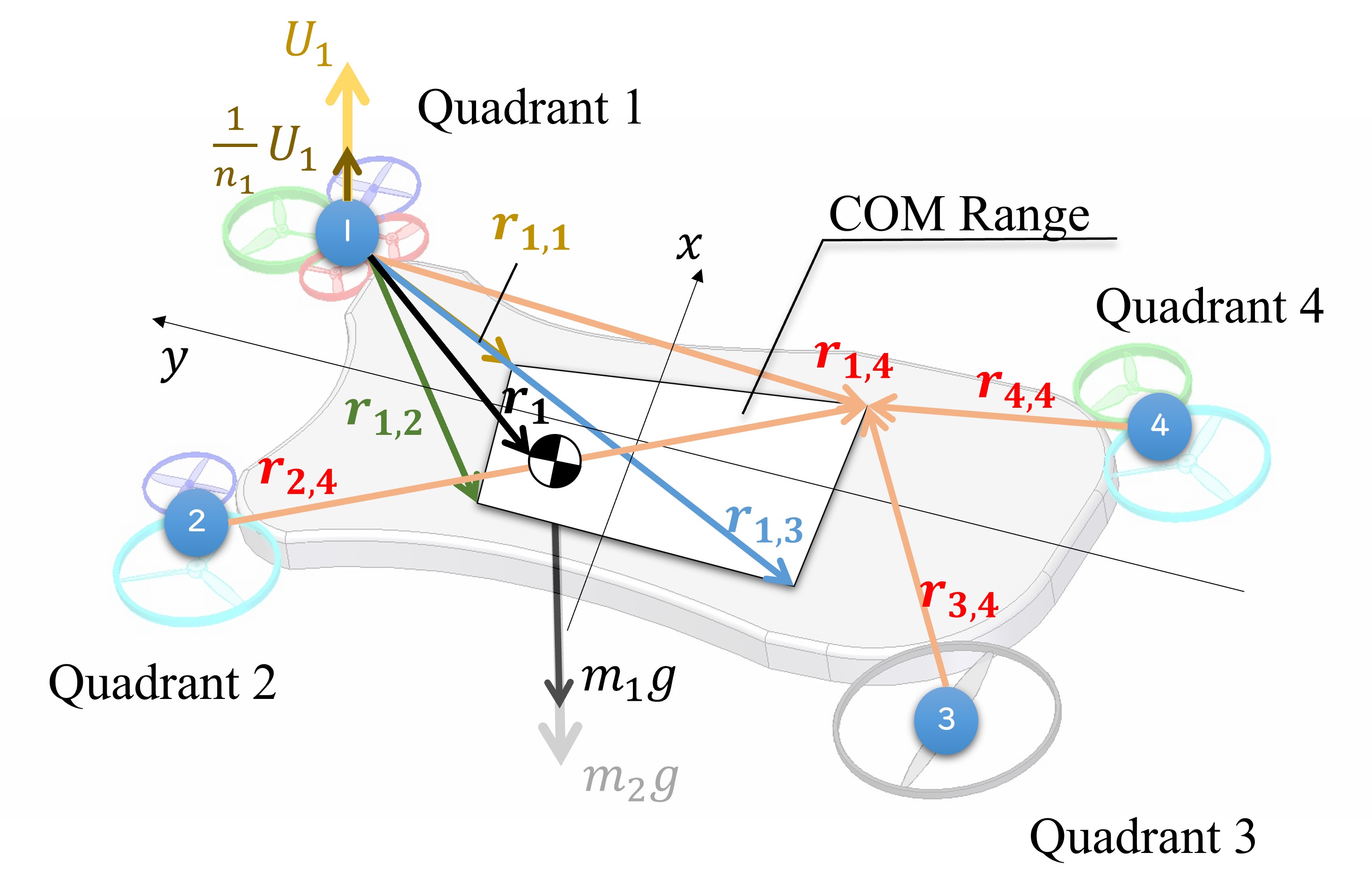
Figure 3: Polytope model

4.1.4 Uncertainty sharing

The fluctuations of mass and COM and robot failures are treated as a change in the $\bm{B}$, as described in Section 3. The fluctuation range is assumed to be known, as shown in Fig. 3. Furthermore, our method is based on the assumption that the thrust loss per robot failure is $\frac{1}{n_{i}}U_{i}$ in quadrant $i$. This assumption is realistic because aerial systems cannot fly beyond their physical limits. The design of the RFC can be simplified if these fluctuations can be described using polytope expression. Therefore, the uncertainties associated with the mass, the COM, and robot failures are defined as follows:

$$\frac{1}{m}=\sum_{i=1}^{2}\frac{\alpha_{i}}{m_{i}},$$

$$\bm{r_{i}}=\sum_{j=1}^{4}\beta_{j}\bm{r_{i,j}},$$

$$U_{i}\rightarrow\left(\sum_{k_{i}=1}^{2}\gamma_{i,k_{i}}b_{i,k_{i}}\right)U_{i},$$

where $m_{1}$ is the expected minimum mass and $m_{2}$ is the expected maximum mass. Furthermore, according to the assumption, $u_{i}=u_{i}^{j}$, $b_{i,1}=\frac{1}{n_{i}}$, and $b_{i,2}=1$. Moreover, the sum of each coefficient is as follows:

$$\begin{split}\sum_{i=1}^{2}\alpha_{i}&=\sum_{j=1}^{4}\beta_{j}=\sum_{k_{1}=1}^{2}\gamma_{1,k_{1}}=\sum_{k_{2}=1}^{2}\gamma_{2,k_{2}}\\ &=\sum_{k_{3}=1}^{2}\gamma_{3,k_{3}}=\sum_{k_{4}=1}^{2}\gamma_{4,k_{4}}=1.\end{split}$$

Note that for $\bm{B}$:

$$\begin{split}&\bm{B_{x}}=\sum_{i=1}^{2}\alpha_{i}\bm{B_{xi}},\\ &\bm{B_{\phi}}=\sum_{i=j}^{4}\beta_{j}\bm{B_{\phi j}}.\\ \end{split}$$

Therefore, $\bm{B}$ can be described in a polytopic form as follows:

$$\begin{split}\bm{B}=\sum_{i=1}^{2}\sum_{j=1}^{4}&\sum_{k_{1}=1}^{2}\sum_{k_{2}=1}^{2}\sum_{k_{3}=1}^{2}\sum_{k_{4}=1}^{2}\\ &\alpha_{i}\beta_{j}\gamma_{1,k_{1}}\gamma_{2,k_{2}}\gamma_{3,k_{3}}\gamma_{4,k_{4}}\bm{B_{ijk_{1}k_{2}k_{3}k_{4}}},\end{split}$$

where $\bm{B_{ijk_{1}k_{2}k_{3}k_{4}}}$ is as follows:

$$\bm{B_{ijk_{1}k_{2}k_{3}k_{4}}}=\left[\begin{array}[]{c}\bm{0_{3\times 4}}\\ \bm{B_{Xi}}\\ \bm{0_{3\times 4}}\\ \bm{B_{\phi j}}\\ \end{array}\right]{\rm diag}\left(b_{1,k_{1}},b_{2,k_{2}},b_{3,k_{3}},b_{4,k_{4}}\right),$$

where $\bm{B_{Xi}}$ and $\bm{B_{\phi j}}$ are as follows:

$$\begin{split}&\bm{B_{Xi}}=\frac{1}{m_{i}}\left[\begin{array}[]{cccc}\bm{e_{3}}&\bm{e_{3}}&\bm{e_{3}}&\bm{e_{3}}\\ \end{array}\right]\in\mathbb{R}^{3\times 4}\\ &\bm{B_{\phi j}}=\bm{J}^{-1}\\ &\left[\begin{array}[]{cccc}(\bm{r_{1,j}}\times\bm{e_{3}})_{12}&(\bm{r_{2,j}}\times\bm{e_{3}})_{12}&(\bm{r_{3,j}}\times\bm{e_{3}})_{12}&(\bm{r_{4,j}}\times\bm{e_{3}})_{12}\\ d_{1}c_{q}&d_{2}c_{q}&d_{3}c_{q}&d_{4}c_{q}\\ \end{array}\right]\\ &\>\>\>\in\mathbb{R}^{3\times 4}.\end{split}$$

Additionally, we assumed that the effect of inertia fluctuations is small.

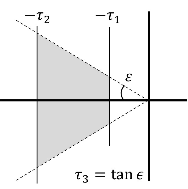
Figure 4: LMI constraint

4.1.5 RFC

Let us derive a feedback gain for a system consisting of eqs. (4) and (9) such that it becomes SPR. First, to increase the flexibility in design, $\bm{G}\in\mathbb{R}^{4\times 4}$ is introduced for eq. (9), and a new output equation is expressed as follows:

$$\bm{\eta}=\bm{G}\bm{\zeta}.$$ (10)

For a system consisting of eq. (4) and eq. (10) to be SPR, it is sufficient that a $\bm{F}$, $\bm{G}$, and positive definite symmetric matrix $\bm{P}$ exist satisfying the following conditions.

$$\begin{split}&\bm{P}(\bm{A}-\bm{B}\bm{F})+(\bm{A}-\bm{B}\bm{F})^{\top}\bm{P}+\\ &\quad(\bm{P}\bm{B}-(\bm{G}\bm{C})^{\top})(\bm{G}\bm{D}+(\bm{G}\bm{D})^{\top})^{-1}\times\\ &\quad\quad(\bm{P}\bm{B}-(\bm{G}\bm{C})^{\top})^{\top}\prec 0,\end{split}$$ (11)

$$\bm{G}\bm{D}+(\bm{G}\bm{D})^{\top}\succ 0.$$ (12)

LMI is a method for solving such matrix inequalities [40]. However, the conditions (11) and (12) cannot be solved directly by LMI. Therefore, the conditions (11) and (12) are converted into the following.

$$\left[\!\begin{array}[]{cc}\bm{A}\bm{Q}\!+\!\bm{Q}\bm{A}^{\top}\!\!-\!\bm{B}\bm{R}\!-\!\bm{R}^{\top}\bm{B}&\bm{Q}\bm{C}^{\top}\!\!-\!\bm{B}\bm{S}^{\top}\\ \bm{C}\bm{Q}\!-\!\bm{S}\bm{B}^{\top}&-\bm{D}\bm{S}^{\top}\!\!-\!\bm{S}\bm{D}^{\top}\\ \end{array}\!\right]\prec 0,$$ (13)

where $\bm{Q}(=\bm{P}^{-1})\in\mathbb{R}^{12\times 12}$, $\bm{R}(=\bm{F}\bm{Q})\in\mathbb{R}^{4\times 12}$, and $\bm{S}(=\bm{G}^{-1})\in\mathbb{R}^{4\times 4}$. Moreover, constraints are introduced to maintain the polar range and $\bm{F}$ small to the highest extent possible as an infinite number of $\bm{F}$ and $\bm{G}$ satisfy eq.(13), as shown in Fig. 4. The pole constraints are as follows:

$$\bm{A}\bm{Q}\!+\!\bm{Q}\bm{A}^{\top}\!\!-\!\bm{B}\bm{R}\!-\!\bm{R}^{\top}\bm{B}+2\tau_{1}\bm{Q}\prec 0,$$ (14)

$$\bm{A}\bm{Q}\!+\!\bm{Q}\bm{A}^{\top}\!\!-\!\bm{B}\bm{R}\!-\!\bm{R}^{\top}\bm{B}+2\tau_{2}\bm{Q}\succ 0,$$ (15)

$$\left[\!\begin{array}[]{cc}\tau_{3}\left(\bm{A}\bm{Q}+\bm{Q}\bm{A}^{\top}\right)&\bm{A}\bm{Q}-\bm{Q}\bm{A}^{\top}\\ \bm{Q}\bm{A}^{\top}-\bm{A}\bm{Q}&\tau_{3}\left(\bm{A}\bm{Q}+\bm{Q}\bm{A}^{\top}\right)\\ \end{array}\!\right]\prec 0.$$ (16)

$\bm{F}$ constraint is as follows:

$$\begin{split}&\min\kappa\\ &s.t.\\ &\bm{Q}\succ\bm{I}\\ &\left[\!\begin{array}[]{cc}\kappa^{2}&\bm{R}^{\top}\\ \bm{R}&\bm{I}\\ \end{array}\!\right]\succ 0.\\ \end{split}$$ (17)

4.2 Asymptotically stabilization

Equilibrium is maintained using the VG-ASSC consisting of variable gains based on $\zeta$ of eq. (9) [2]. However, as eq. (9) includes the control input $\bm{U}$ in addition to the broadcast $\xi$, controlling distribution is challenging. Therefore, first, a method of removing the control input from the output using each acceleration is described.

4.2.1 Output approximation

We consider an approximation of $\bm{U}$ contained in eq. (9). Focusing on $z_{e}$ and $\bm{\phi_{e}}$ in eq. (4), the term $\bm{U}$ can be removed from the equation as follows:

$$\left[\begin{array}[]{c}\ddot{z_{e}}\\ \ddot{\bm{\phi_{e}}}\\ \end{array}\right]=\left[\begin{array}[]{c}\frac{\bm{1_{4}}^{\top}}{m}\\[5.0pt] \bm{B_{\phi}}\\ \end{array}\right]\left(\bm{U}-\bm{U_{r}}\right),$$

where $\bm{1}_{4}^{\top}=[1,1,1,1]$. Thus, $\bm{U}-\bm{U_{r}}$ is as follows:

$$\bm{U}-\bm{U_{r}}=\left[\begin{array}[]{c}\frac{\bm{1_{4}}^{\top}}{m}\\[5.0pt] \bm{B_{\phi}}\\ \end{array}\right]^{-1}\left[\begin{array}[]{c}\ddot{z_{e}}\\ \ddot{\bm{\phi_{e}}}\\ \end{array}\right].$$

Then, eq. (10) is converted as follows:

$$\bm{\eta}=\bm{G}\bm{C}\bm{\xi}+\bm{G}\bm{\hat{D}}\left[\begin{array}[]{c}\ddot{z_{e}}\\ \ddot{\bm{\phi_{e}}}\\ \end{array}\right],$$ (18)

where $\bm{\hat{D}}$ is as follows:

$$\bm{\hat{D}}=\bm{D}\left[\begin{array}[]{c}\frac{\bm{1_{4}}^{\top}}{m}\\[5.0pt] \bm{B_{\phi}}\\ \end{array}\right]^{-1}.$$

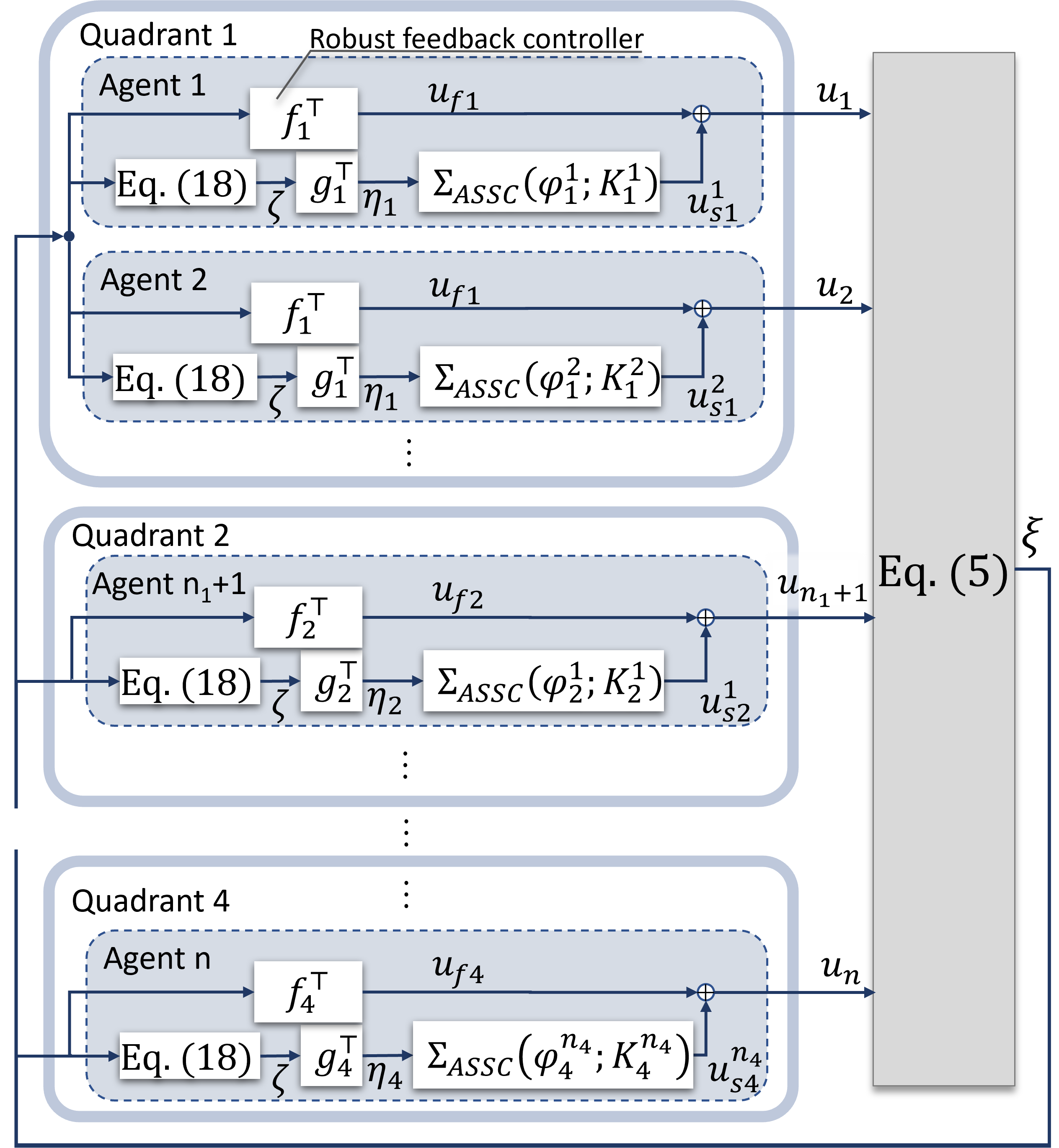
Figure 5: Proposed controller

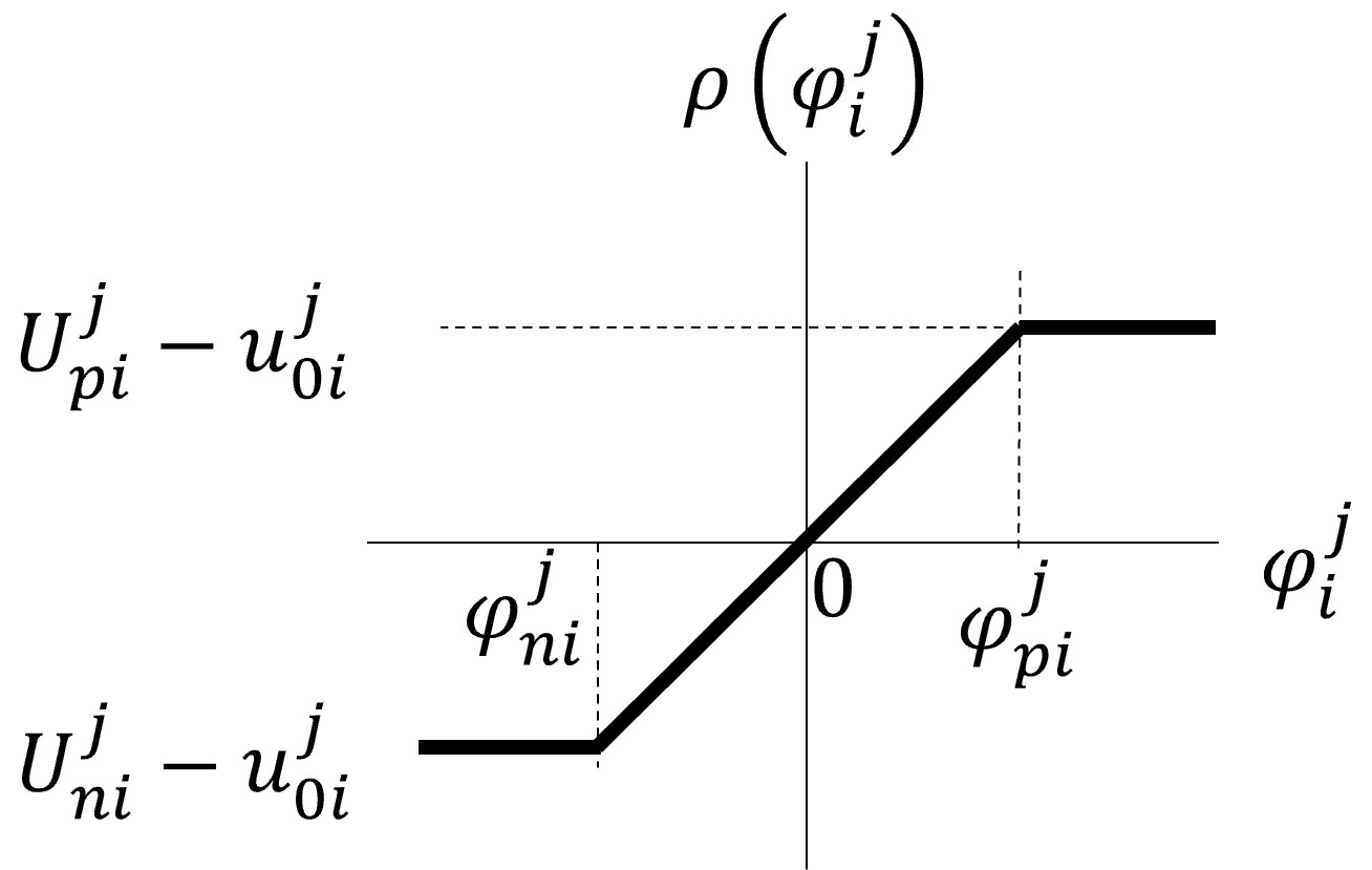
Figure 6: Switching function $\rho$ [25]

4.2.2 VG-ASSC

VG-ASSC control is based on the $\eta$ of eq. (18), as shown in Fig. 5. Unlike the RFC, the VG-ASSC can use individual control for each robot. Therefore, $\hat{\eta}$, which is $\eta$ extended by the number of robots, is defined as follows:

$$\hat{\eta}=\left[\begin{array}[]{c}\bm{\hat{\eta}^{1}}\\ \bm{\hat{\eta}^{2}}\\ \bm{\hat{\eta}^{3}}\\ \bm{\hat{\eta}^{4}}\\ \end{array}\right],$$ (19)

where $\bm{\hat{\eta}^{1}_{i}}=[\eta_{1},\dots,\eta_{1}]\in\mathbb{R}^{n1}$, $\bm{\hat{\eta}^{2}_{i}}=[\eta_{2},\dots,\eta_{2}]\in\mathbb{R}^{n2}$, $\bm{\hat{\eta}^{3}_{i}}=[\eta_{3},\dots,\eta_{3}]\in\mathbb{R}^{n3}$, and $\bm{\hat{\eta}^{4}_{i}}=[\eta_{4},\dots,\eta_{4}]\in\mathbb{R}^{n4}$. The non-linear variable gain of VG-ASSC featuring using this $\bm{\hat{\eta}}$ is as follows:

$$\begin{split}\Sigma_{\rm{ASSC}}&\left\{\begin{array}[]{l}\dot{\varphi}_{i}^{j}=-K_{i}^{j}(\varphi_{i}^{j},\hat{\eta}_{i}^{j})\hat{\eta}_{i}^{j}\\[3.0pt] u_{si}^{j}=\rho(\varphi_{i}^{j})+u_{0i}\end{array}\right.,\\[5.0pt] \rho(\varphi_{i}^{j})=&\left\{\begin{array}[]{l}U_{pi}^{j}-u_{0i}^{j}:\varphi_{i}^{j}>\varphi_{pi}^{j}\\[3.0pt] U_{pi}^{j}\varphi_{i}^{j}:\varphi_{ni}^{j}<\varphi_{i}^{j}\leq\varphi_{pi}^{j}\\[3.0pt] U_{ni}^{j}-u_{0i}^{j}:\varphi_{i}^{j}\leq\varphi_{ni}^{j}\end{array}\right.,\end{split}$$ (20)

where $K_{i}^{j}>0$ are the gains; $u_{si}^{j}$ is the control input of the ASSC of robot $j$ in quadrant $i$; $U_{pi}^{j}$ and $U_{ni}^{j}$ are the upper and lower limits of the thrust applied by the robot, respectively; $\rho$ is the switching function of $\varphi_{i}^{j}$, as shown in Fig. 6; $\varphi_{pi}^{j}$ is $\varphi_{i}^{j}$ with $U_{pi}^{j}\varphi_{i}^{j}=U_{pi}^{j}-u_{0i}$; $\varphi_{ni}^{j}$ is $\varphi_{i}^{j}$ with $U_{ni}^{j}\varphi_{i}^{j}=U_{ni}^{j}-u_{0i}$, and $u_{0i}^{j}$ is the thrust for hovering. Notably, $\varphi_{pi}^{j}+\varphi_{ni}^{j}=1$. Moreover, $K_{i}^{j}$ can be expressed as follows:

$$\begin{split}K_{i}^{j}(\varphi_{i}^{j},\hat{\eta}_{i}^{j})=\left\{\begin{array}[]{l}\overline{k_{i}}^{j}:\varphi_{i}^{j}\hat{\eta}_{i}^{j}>0\\[4.0pt] \underline{k_{i}}^{j}:\varphi_{i}^{j}\hat{\eta}_{i}^{j}\leq 0\end{array}\right.\\ \end{split}$$ (21)

where $\overline{k_{i}}^{j}$ and $\underline{k_{i}}^{j}$ are positive values satisfying $0<\underline{k_{i}}\leq\overline{k_{i}}$.

Theorem 1.

Applying the controller of eq. (20) to the error system comprising eqs. (4) and (18) shows that the error $\hat{\bm{\eta}}$ satisfies $\hat{\bm{\eta}}\rightarrow 0$ as $t\rightarrow\infty$.

Proof.

See Appendix A for the proof. ∎

This controller adds multiple outputs and offsets $u_{oi}^{j}$ to the controller of Amano et al. [2]. Multiple outputs and offsets are necessary to handle aerial systems. $\varphi_{i}^{j}$ is almost positive, and variable gain is not effective because the aerial system needs to apply thrust continuously. Therefore, an offset term $u_{0i}^{j}$ is introduced.

High-response decentralized control can be expected by our controller. $\varphi_{i}^{j}$ is 0 at ideal equilibrium due to $u_{0i}^{j}$. $u_{si}^{j}$ applies thrust in the opposite direction of the integral of $\hat{\eta}_{i}^{j}$. Thus, eq. (20) temporarily gives the control input in the opposite direction to the desired control input when $\varphi_{i}^{j}\hat{\eta}_{i}^{j}$ is positive. Therefore, the response can be improved by providing a considerable gain when $\varphi_{i}^{j}\hat{\eta}_{i}^{j}$ is positive.

5 Numerical simulation

As detailed in this section, the proposed and PID controllers are compared using numerical simulation. We simulated the transportation of a rectangular-shaped payload using eight single-rotor robots and the transportation of an L-shaped payload using ten robots. In addition, the single-rotor robots use three types of robots with different maximum thrusts. The proposed controller is designed to be robust against fluctuations of mass and COM and robot failures by utilizing the method described in Section 4.1.5.

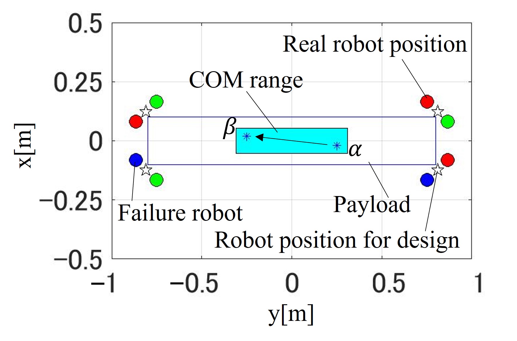
(a) Rectangle-shape

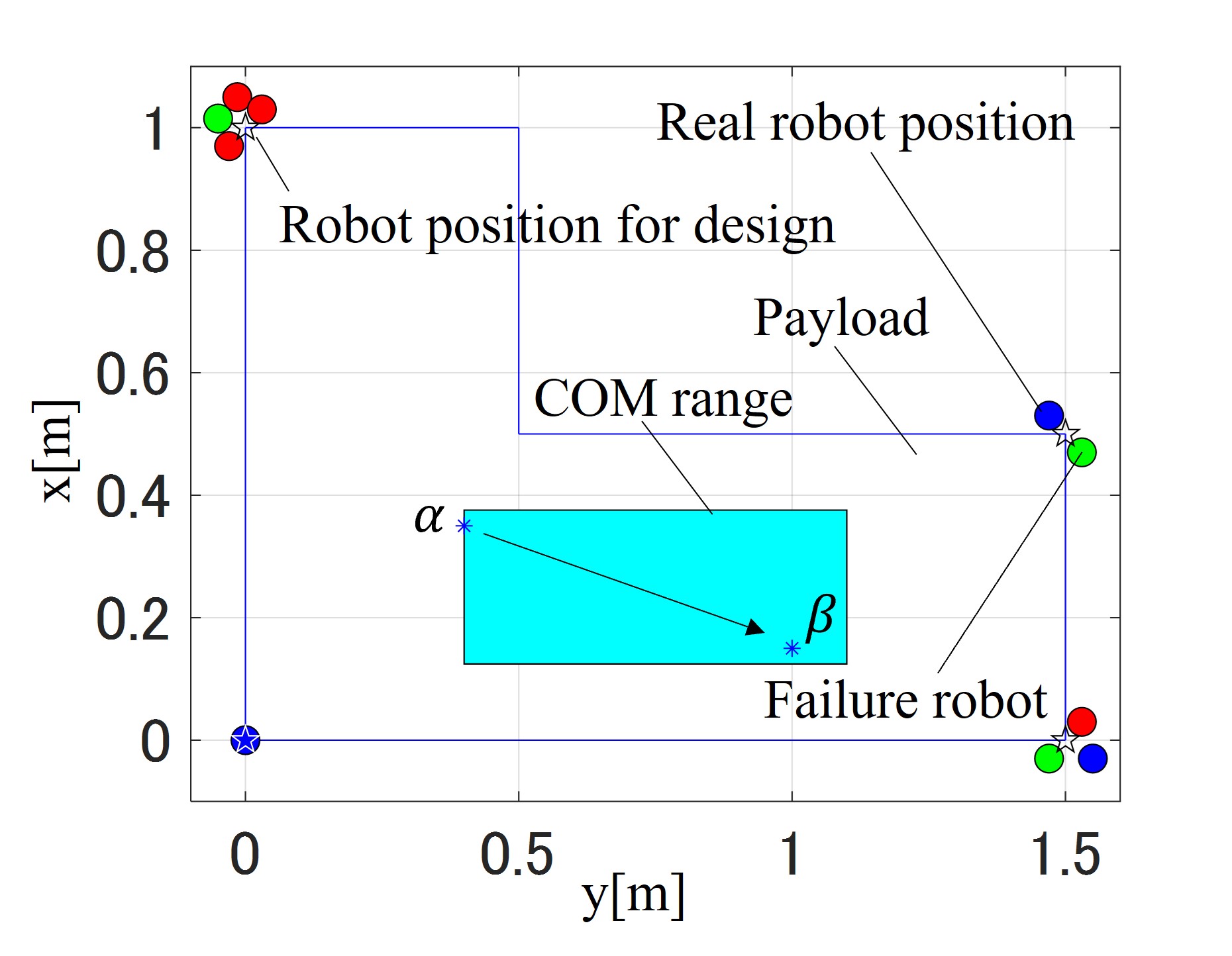
(b) L-shape

Figure 7: Two different shapes of payloads used for the simulations. The blue line indicates the shape of the payload, filled circles indicate the actual robot positions, red filled circles indicate Robot A, green filled circles indicate Robot B, blue filled circles indicate Robot C, stars indicate robot positions for the control design, filled area indicates the COM range, and asterisks indicate the simulated COM positions.

Table 1: Control parameters of simulation

Parameter	Rectangle-shape	L-shape
$n_{1}$, $n_{2}$, $n_{3}$, $n_{4}$	$2$, $2$, $2$, $2$	$4$, $2$, $3$, $1$
$m_{1}$,$m_{2}$	$2$, $5.5$ kg	$2$, $5.5$ kg
$c_{q}$	$0.162$	$0.162$
$J$	$\rm{diag}\left(\left[0.419,0.010,0.429\right]\right)$ $\rm{kgm}^{2}$	$\rm{diag}\left(\left[0.392,0.142,0.521\right]\right)$ $\rm{kgm}^{2}$
$[c_{x0},c_{x1},c_{x2},c_{x3},c_{x4}]$	$[1.00,2.20,1.82,0.67,0.09]$	$[1.00,2.00,1.5,0.5,0.06]$
$[c_{y0},c_{y1},c_{y2},c_{y3},c_{y4}]$	$[1.00,2.00,1.5,0.5,0.06]$	$[1.00,2.00,1.5,0.5,0.06]$
$[c_{z0},c_{z1},c_{z2}]$	$[1.00,1.00,0.25]$	$[1.00,1.00,0.25]$
$[c_{\psi 0},c_{\psi 1},c_{\psi 2}]$	$[1.00,1.00,0.25]$	$[1.00,1.00,0.25]$
$[\tau_{1},\tau_{2},\tau_{3}]$	$[0.25,140,1.00]$	$[0.40,60.0,0.60]$
$\overline{k}$	$49$	$49$
$\underline{k}$	$7$	$7$

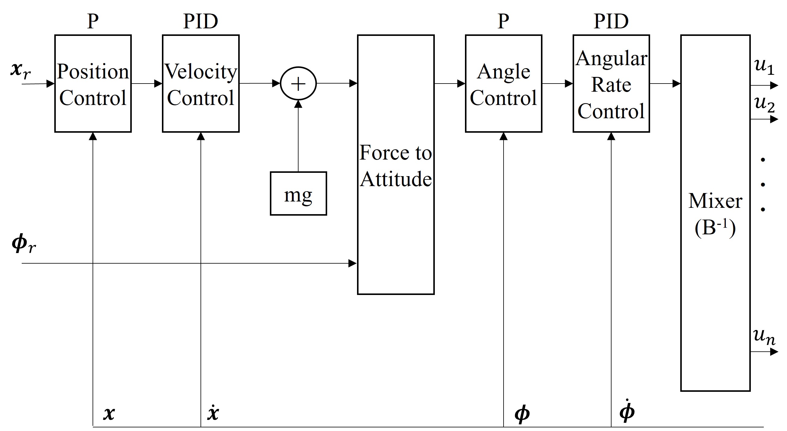
Figure 8: Conventional PID controller

Table 2: Simulation conditions

Condition	Value
Initial position	$\left[0,0,2\right]$ m
Initial attitude	$\left[0,0,0\right]$ rad
Target position	$\left[2,0,2\right]$ m
Target attitude	$\left[0,0,0\right]$ rad
Time to give command	$30$ s
Time to give COM fluctuations ($t_{c}$)	$50$ s
Time to give failure ($t_{f}$)	$60$ s
Initial mass	$3.0$ kg
Mass after fluctuations	$4.0$ kg
Motor time constant	$0.01$ s
Time step	$10$ µs

5.1 Condition

In this simulation, we used three robots, designated A, B, and C, with different maximum thrusts of 7, 12, and 15 Nm, respectively. A configuration of simulation targets is shown in Fig.7. The rectangular shape is similar to the prototype described in Section 6. The arrows in the figure indicate the movement of the COM during the simulation. The parameters used for the controller design are shown in Table 1. Moreover, VG-ASSC requires an equilibrium thrust of $u_{0i}^{j}$. However, $u_{0i}^{j}$ is unknown at the time of design. Therefore, the initial values are given by equally distributing $3.5$ kg, which is the average of the mass design range, among the robots. Thus, the robots use fixed gain instead of variable gain until they obtain the true $u_{0i}^{j}$. The fixed gain at this time is $\underline{k}_{i}^{j}$. In addition, the $\overline{k}_{i}^{j}$ and $\underline{k}_{i}^{j}$ of all robots are the same. The PID control for comparison was the general cascade PID shown in Fig. 8 [23]. The parameters of the PID controller were set such that the difference in response time from the proposed control would be 10 % when the reference value given a step under the COM was the center and the mass was 3.5 kg. Appendix B provides further details regarding the parameters.

The task in the simulation is to move from an initial position in mid-air to a target position. The target position is given as a reference. The VG-ASSC requires the thrust $u_{0i}^{j}$ of each robot during hovering as a control parameter. Therefore, the thrust at 18 s is obtained as $u_{0i}^{j}$. Subsequently, the target position is given at 30 s, and fluctuations of COM and mass are given at 50 s ($t_{c}$). In addition, the robot failure is given at 60 s ($t_{f}$). Simulation parameters are shown in Table 2. Furthermore, if the pitch or roll angle exceeds 90^∘, it is considered to have crashed.

The simulation is performed with a model in which the Coriolis force and a first-order approximation of the motor are added to eq. (1). Additionally, the time step is ten microseconds, which is well ahead of the system’s response.

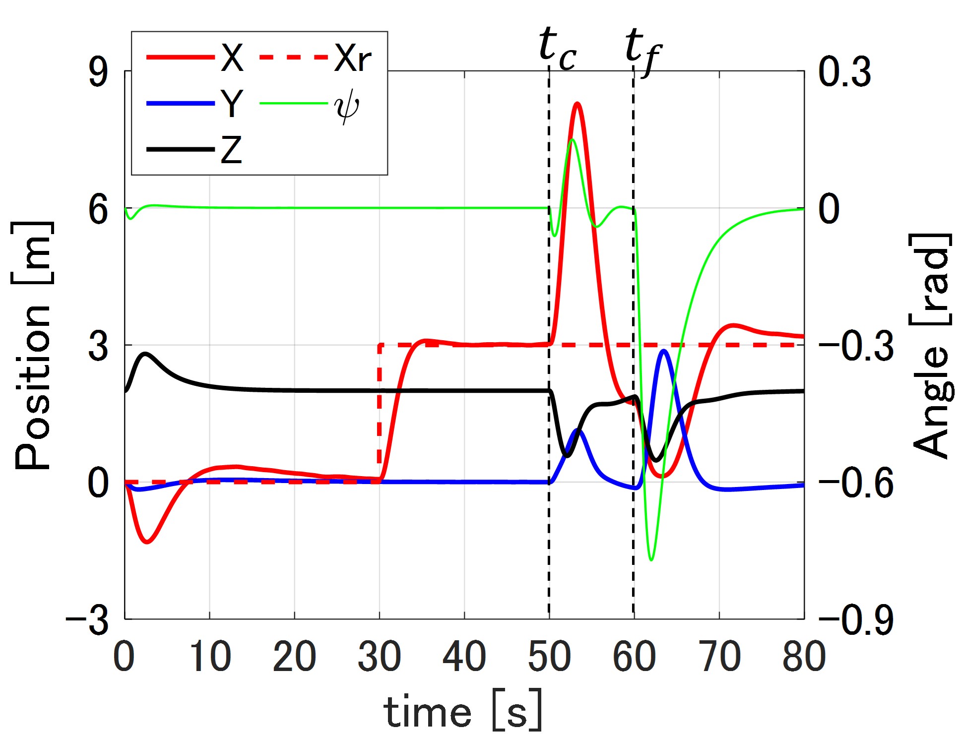
(a) PID controller

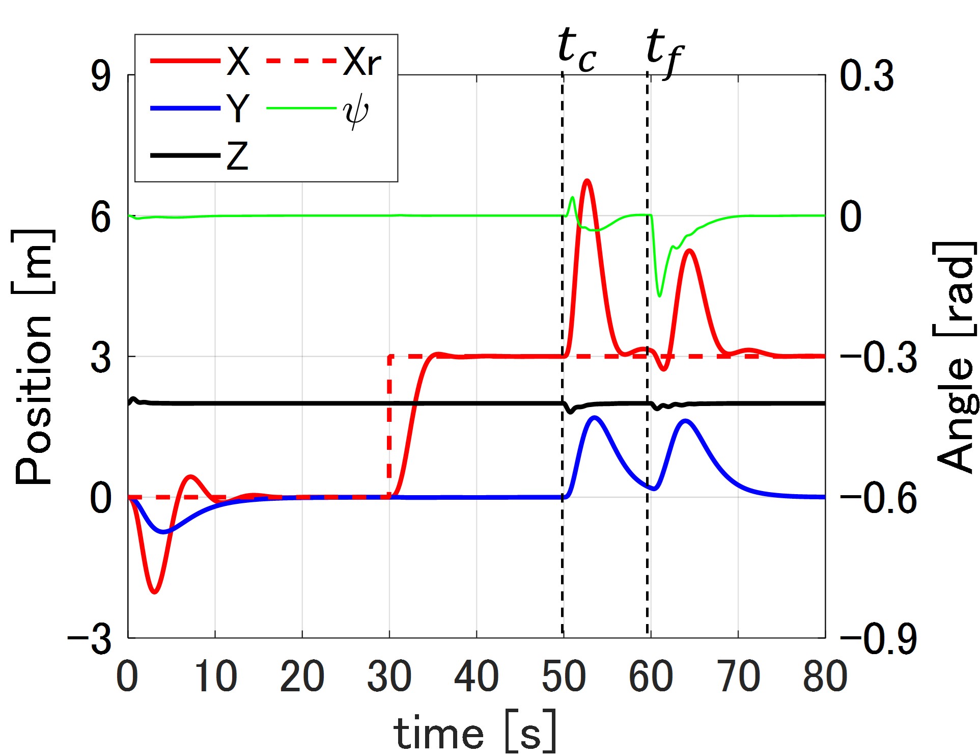
(b) Variable gain ASSC

Figure 9: Time series of the position, yaw angle, and reference of the rectangular-shaped payload with fluctuations of mass and COM and robot failure using two controllers. $Xr$ denotes reference of $X$. The vertical axis on the left indicates the positions and the vertical axis on the right indicates a yaw angle.

5.2 Result

The simulation results with the rectangular- and L-shaped payloads are shown in Fig. 9 and Fig. 10, respectively. The proposed controller has a smaller payload position and yaw angle fluctuations for both the rectangular- and L-shaped than PID controller. In particular, the PID controller crashes at time 59 s, whereas the ASSC-based controllers keep flying in the case of the L-shaped. Therefore, the proposed controller is expected to be adaptable to changes in geometry and the number of robots and can be robust against fluctuations.

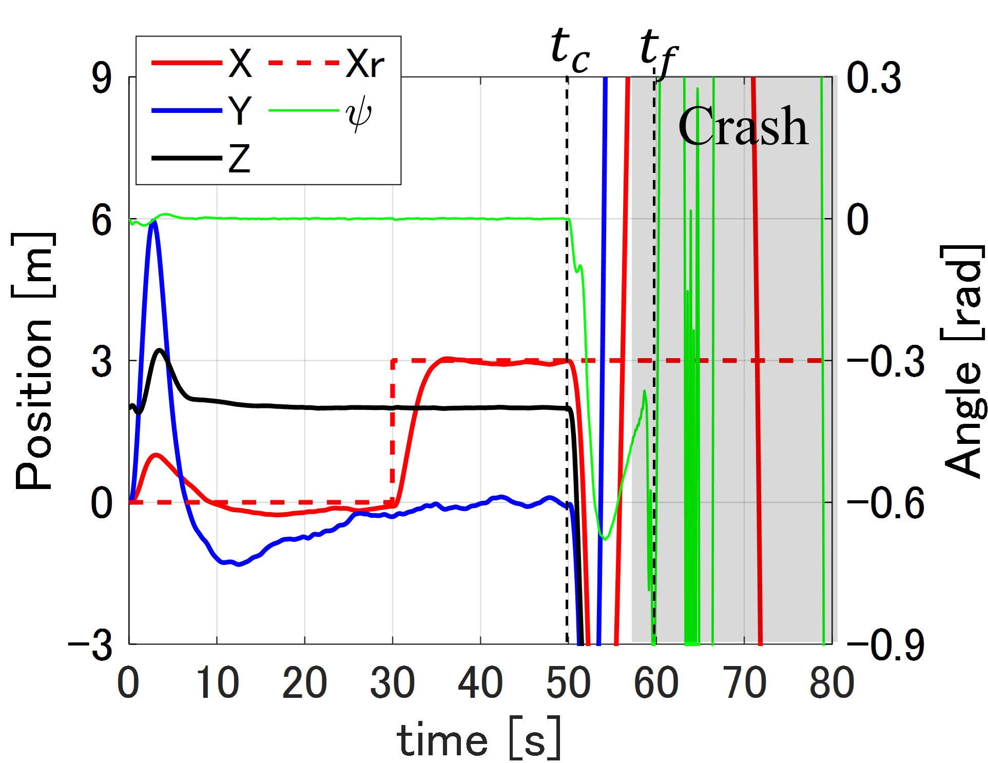
(a) PID controller

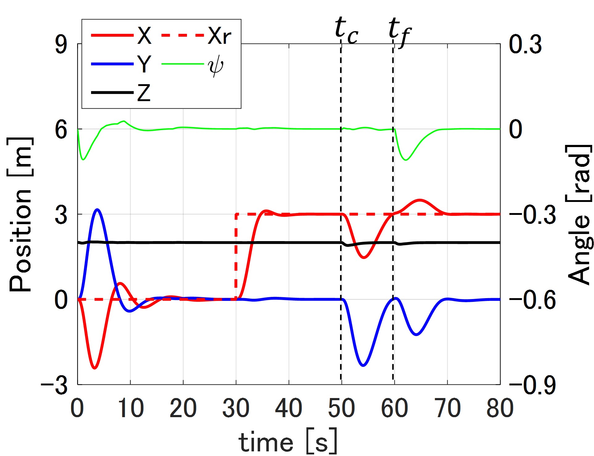
(b) Variable gain ASSC

Figure 10: Time series of the position, yaw angle, and reference of the L-shaped payload with fluctuations of mass and COM and robot failure using two controllers. Each display is the same as that shown in Fig.9.

6 Real robot experiment

This section presents the implementation of the proposed method on a prototype consisting of various types of single-rotor robots and verification of the feasibility of aerial transportation. The prototype has a rectangular-shaped payload and eight single-rotor robots. The experiment moves from takeoff to destination with fluctuations.

6.1 Prototype

The prototype consists of eight robots, a rectangular-shaped payload, and ball robots that simulate changes in the COM, as shown in Fig.11. In addition, the eight robots consist of three types of robots: robot $\rm{A}^{\prime}$, robot $\rm{B}^{\prime}$, and robot $\rm{C}^{\prime}$. Each robot is distributed and controlled by its independent controller, as mentioned in section 4.2.2. However, the controller of the prototype is independent only within the software to facilitate production. Therefore, as regards the hardware, each robot is controlled by one controller mounted on the payload. The controller hardware is PIXHAWK [19]. The software for the controller was coded using MATLAB^® Simulink^®, and Stateflow^® and was implemented using PX4 Autopilots Support from UAV Toolbox. Each position, velocity, and yaw angle were acquired using a motion capture system, and other states were acquired using the existing estimator from the sensors in the controller [19]. Furthermore, the prototype has a space for the ball robots to move for COM fluctuations on the top of the payload. SPRK+ was used for the ball robots [39]. The range of COM change by the ball robots is $0.12$ m on the left and $0.03$ m on the right, as shown in Fig. 11. The offset to the left is the effect of the mounted camera for photographing the robot failure. In this experiment, the ball robots were remotely controlled at a certain time to imitate the fluctuation of the COM. In addition, failure was imitated by forcibly setting the thrust command of the single-rotor robot to $0$. The specifications of the prototype are shown in Table 3.

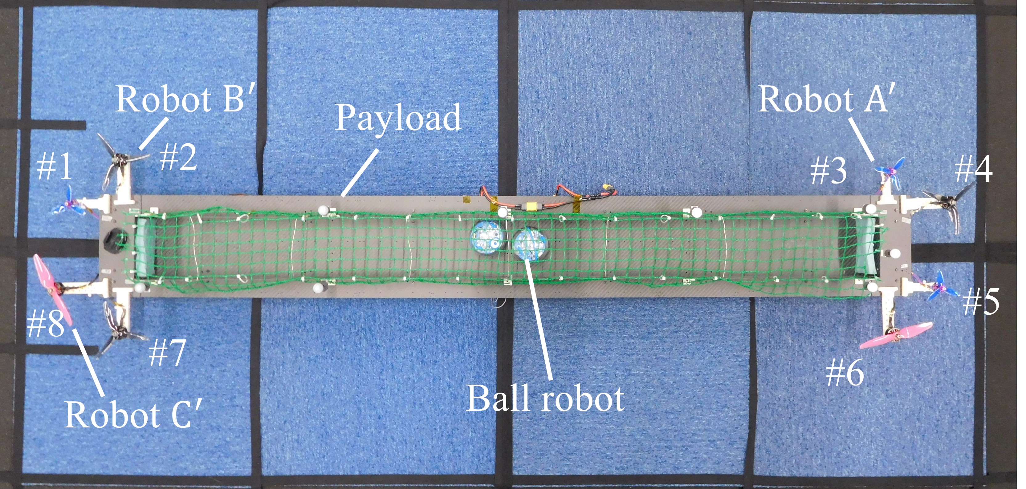
Figure 11: Prototype

Table 3: Prototype specifications

Payload
Mass (with all robots)	$2.2$ kg
Size (without robots)	$1.6$ $\times$ $0.2$ m
Mass of battery	$0.432.6$ g
Inertia($[\bm{J_{xx}},\bm{J_{yy}},\bm{J_{zz}}]$)	$\left[0.419,0.010,0.429\right]$ $\rm{kgm}^{2}$
Mass of Ball robot	$0.18$ kg
Mass of camera	$0.18$ kg
Robot $\rm{A}^{\prime}$
Motor KV	$4200$ KV
Propeller	$3$ inch, $3$ blades
Max-thrust (catalog value)	$6.0$ N ($0.61$ kgf)
Robot $\rm{B}^{\prime}$
Motor KV	$2400$ KV
Propeller	$5$ inch, $3$ blades
Max-thrust (catalog value)	$14.2$ N ($1.45$ kgf)
Robot $\rm{C}^{\prime}$
Motor KV	$2500$ KV
Propeller	$6$ inch, $2$ blades
Max-thrust (catalog value)	$16.7$ N ($1.7$ kgf)

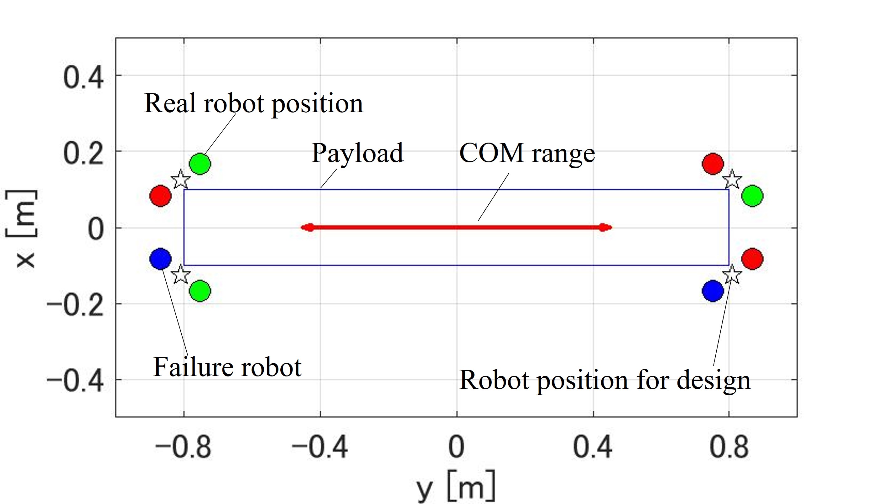
Figure 12: Robot position and COM range on control design and failure robot. Filled circles indicate the actual robot positions, red filled circles indicate Robot ‘A’, green filled circles indicate Robot ‘B’, blue filled circles indicate Robot C’, and stars indicate robot positions for the control design.

Table 4: Control parameters of real robot experiment

Parameter	Prototype
$n$	$8$
$m$	$3.06$ kg
$c_{q}$	$0.162$
$\bm{J}$	$\rm{diag}\left(\left[0.419,0.010,0.429\right]\right)$ $\rm{kgm}^{2}$
$\left[c_{x0},c_{x1},c_{x2},c_{x3},c_{x4}\right]$	$\left[1,4,3,1,0.01\right]$
$\left[c_{y0},c_{y1},c_{y2},c_{y3},c_{y4}\right]$	$\left[1,3,3,0.2,0.01\right]$
$\left[c_{z0},c_{z1},c_{z2}\right]$	$\left[1,0.8,0.05\right]$
$\left[c_{\psi 0},c_{\psi 1},c_{\psi 2}\right]$	$\left[1,7,0.25\right]$
$\left[\tau_{1},\tau_{2},\tau_{3}\right]$	$\left[0.1,18,2\right]$
$\overline{k}$	$4.5$
$\underline{k}$	$1.5$

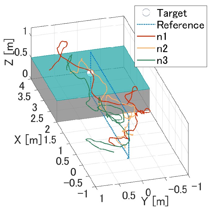
(a) Trajectory

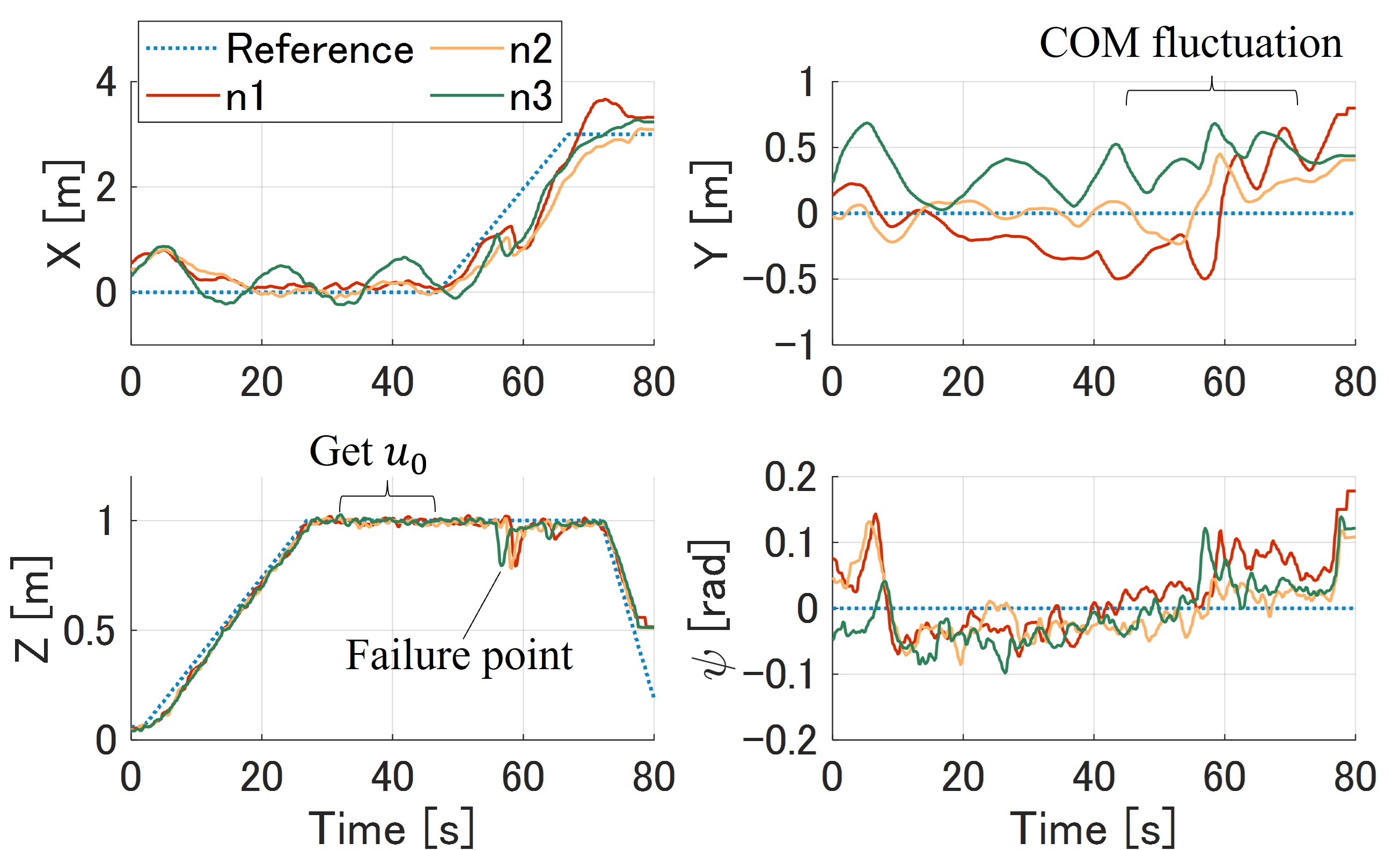
(b) Time series of position and yaw angle

Figure 13: Payload positions and yaw angle during experiments with the fluctuations. Dotted lines represent the reference trajectory, and solid lines represent the actual positions.

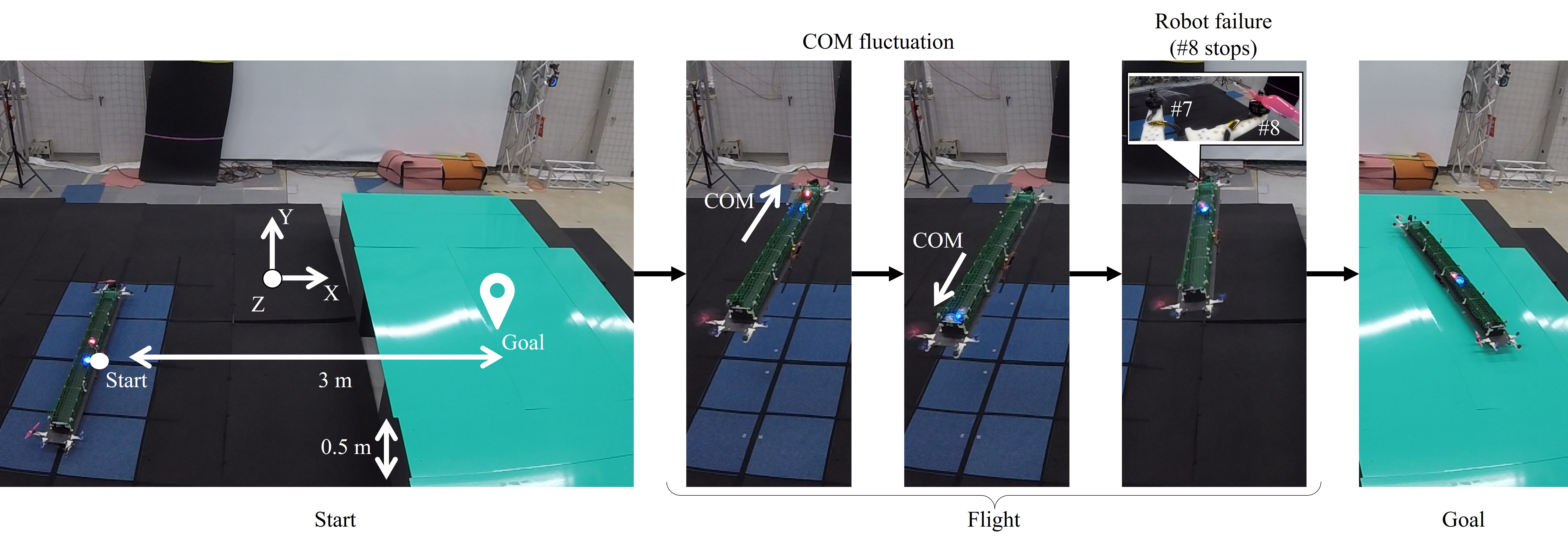
Figure 14: Experiment using prototype

6.2 Condition

The task of the real experiment comprised the transportation to the target positions and the disturbances. The controller was designed to be robust against fluctuations of COM and robot failure because mass fluctuation could not easily be imitated in real experiments. The fluctuation range of the COM for design was limited to the longitudinal direction because the COM of prototype fluctuates in the longitudinal direction, as shown in Fig. 12. The representative point of robot positions for design was set to the midpoint of the straight line connecting robots in each quadrant. The parameters in the control design are shown in Table 4. The initial values of $u_{0i}^{j}$ were determined by equally distributing $3.06$ kg, which is the average of the mass, among the robots. The true value of $u_{0i}^{j}$ was obtained during hovering.

The transportation tasks in this experiment included takeoff, hovering in the air, and landing at the target position. Specifically, the payload was hovered at an altitude of 1 m, then moved 3 m in the $X$ direction, and landed on a 0.5-m-high platform. The reference value $\bm{x_{r}}$ for performing this operation was continuously and automatically given. Furthermore, the controller used $\underline{k}$ as a fixed gain instead of the variable gain until the true $u_{0i}^{j}$ was obtained during hovering. To obtain $u_{0i}^{j}$, the thrust command of each robot with a 5-Hz low-pass filter was used. In this experiment, for safety, the acquisition of $u_{0i}^{j}$ and robot failure were performed when a signal was remotely sent. In addition, the movement of the ball robots for the change in the COM was performed after obtaining $u_{0i}^{j}$.

6.3 Result

The results of three experiments are shown in Fig. 13. In all three experiments, $u_{0i}^{j}$ was obtained at approximately 40 s, the COM was changed by the ball robots at 50 s when the command in the $X$ direction was given until it reached the goal, and robot failure occurred at approximately 57 s. Fig. 14 shows the flow of the second experiment. Fig. 13(a) and Fig 13(b) show that the proposed controller can perform aerial transportation even with heterogeneous robot configurations. Moreover, the prototype can reach the vicinity of the goal without falling into a fatal state if COM fluctuations and robot failure occur.

7 Discussion

Cooperative transportation by our decentralized controller is possible even with heterogeneous robot configurations under the same constraints as those used in previous research [25]. In addition, the simulations in section 5 suggest that a variety of numbers of robots, which was not mentioned in previous research, can be handled. The constraints used in our approach are more relaxed than those in the approach of [20] and [30] regarding the mass and shape of the payload. For the constraints on the robot position, it is assumed that they are concentrated at representative points in each quadrant as shown in Fig. 3. These constraints are similar to the symmetry arrangement in the approach of [43]. These positional constraints are set because some positional information is required by the controller for guaranteed stability. It is possible to use an approach wherein the robot itself estimates its own position with respect to the payload as a method to relax restrictions on position information [26].

For hardware, we use a single-rotor robot such as the one in [28, 24]. Our study suggests that it is possible to use a modeled aerial robot similar to [24] to perform transportation tasks with distributed controllers and heterogeneous robots. Thus, our proposal further improves the advantages of modular configurations. An aerial robot equipped with a single rotor rather than a multi-copter has a wider range of applications in the case of assuming cooperative flight with multiple robots. This is because a multicopter can be regarded a collection of rotors equipped with one rotor. Connecting with the payload can be a challenging problem in the case of transportation. The connection between single-rotor robots and the payload is screwed in our prototype. This connection should be simplified to render plug-in/plug-out practical. Notably, some methods that can be applied as various grasping mechanisms for multicopters have been proposed in recent years [21].

7.1 Offset error of experiment

The proposed controller can reach the goal even when fluctuations occur. However, an error occurs with respect to the position, as shown in Fig. 13. In particular, an offset error occurs in the $Y$ direction. This error can be the effect of angular offset errors. The broadcast value used by our controller is the sum of the state errors, as shown in eq. (8). States other than $x$, $y$, $z$, and $\psi$ are set to $0$ as the assumption of the equilibrium state because our controller aims to maintain the equilibrium state. However, in a real prototype, errors can occur in part of the state because of sensor errors or distortion of the body even if it is hovering and stationary. Assuming the occurrence of an error $\phi_{d}$ in the longitudinal angle $\phi$, which is particularly prone to distortion, and ignoring the coefficients, $y_{p}$ in eq. (8) in equilibrium state is represented as

$$\begin{split}y_{p}&=\ddddot{y_{e}}+\dddot{y_{e}}+\ddot{y_{e}}+\dot{y_{e}}+y_{e},\\ y_{p}&=-g(\phi_{r}+\phi_{d})-\ddot{y_{r}}+y-y_{r},\\ y_{p}&=-g\phi_{d}+y-y_{r},\end{split}$$

where $\ddddot{y_{e}}=\dddot{y_{e}}=\dot{y_{e}}=0$ and $-g\phi_{r}=\ddot{y_{r}}$ because of the equilibrium state and the assumption. As the controller causes $y_{p}$ to asymptote to 0, $y$ is as follows:

$$y=g\phi_{d}+y_{r}.$$ (22)

An error of $g\theta_{d}$ occurs in $y$ from eq.(22). We introduced a process to eliminate the offset error from the current angle before takeoff even during the real robot experiment. However, the effect is limited because the ground is not horizontal and the prototype is distorted. Alternatively, the value of the acceleration sensor can be used without approximation. However, in this method, a risk of runaway arises when angled while stationary because of ground contact during moments such as landing, as the controllability of the attitude is reduced. This situation can be addressed by switching the state acquisition of the sensor according to the flight state. Furthermore, the timing with the largest error at the $Y$ position in the real robot experiment occurs before landing at the first experiment(n1). This error can be affected by the above-mentioned challenge and the ground effect as the ground effect occurs in the vicinity of the ground. Fishman et al. [10] attempted to solve this ground effect using a deep learning method. However, they failed because of data obtained by issues such as contact near the ground.

8 Conclusion

In this study, we proposed a decentralized cooperative transportation system with heterogeneous single-rotor robots. The proposed method extends plug-in/plug-out, the advantages of decentralized control, to heterogeneous robots for cooperative aerial transportation tasks. Owing to this effect, even deteriorated robots can be reused. In addition, our controller using an RFC and VG-ASSC was robust against fluctuations, and convergence was guaranteed. Using numerical simulation, we confirmed that our system could be transported in the air under significant fluctuations even with different numbers of robots and different payload shapes. In addition, aerial transportation was possible even if a failure and COM shift occurred in real robot experiments using the prototype.

As a future task, the restrictions of this controller must be relaxed. The robot positions are restricted to the vicinity of the representative point for rendering the target system SPR. This restriction is a major limitation as rotor blades are generally large. In the future, we will aim to relax this restriction.

Appendix A Proof of theorem1

The error system consisting of eqs.(4) and (18) can be represented as follows:

$$\begin{array}[]{l}\bm{\dot{\xi}}=\hat{\bm{A}}\bm{\xi}+\bm{B}(\bm{U}-\bm{U_{r}})\\ \bm{\eta}=\bm{G}\bm{C}\bm{\xi}+\bm{G}\bm{\hat{D}}\left[\begin{array}[]{c}\ddot{z_{e}}\\ \ddot{\bm{\phi_{e}}}\\ \end{array}\right]\end{array},$$ (23)

where $\hat{\bm{A}}:=\bm{A}-\bm{B}\bm{F}$. The hyperstability theorem [3, 16] guarantees the asymptotic stability of the error $\hat{\eta}$ if eq.(20) is passive. This is because eq.(23) is SPR by the RFC. Therefore, we show that eq. (20) is passive.

First, eq.(20) is rearranged to improve readability. The maximum and minimum values of $\rho$ are redefined as $\hat{U}_{\text{p}i}:=U_{\text{p}i}-u_{0i}$, $\hat{U}_{\text{n}i}:=U_{\text{n}i}-u_{0i}$. Furthermore, the variable in $rho$ is redefined as $\varphi_{i}:=[\varphi^{1}_{1},\varphi^{1}_{2},\dots,\varphi^{4}_{n_{4}}]^{\top}$, error is redefined as $\hat{\eta}_{i}:=[\eta^{1}_{1},\eta^{1}_{2},\dots,\eta^{4}_{n_{4}}]^{\top}$, control input is redefined as $u_{\text{s}i}:=[u^{1}_{\text{s}1},u^{1}_{\text{s}2},\dots,u^{4}_{\text{s}n_{4}}]^{\top}$, and control gain is redefined as $K_{i}:=[K^{1}_{1},K^{1}_{2},\dots,K^{4}_{n_{4}}]^{\top}$. Thus, eq.(20) can be represented as follows:

$$\begin{split}\Sigma_{\rm{ASSC}}&\left\{\begin{array}[]{l}\dot{\varphi}_{i}=-K_{i}(\varphi_{i},\hat{\eta}_{i})\hat{\eta}_{i}\\ u_{si}=\rho(\varphi_{i})+u_{0i}\end{array}\right.\\ \\ \rho(\varphi_{i})=&\left\{\begin{array}[]{l}\hat{U}_{pi}:\varphi_{i}>\varphi_{\rm{p}i}\\ \hat{U}_{pi}\varphi_{i}:\varphi_{\rm{n}i}<\varphi_{i}\leq\varphi_{\rm{p}i}\\ \hat{U}_{ni}:\varphi_{i}\leq\varphi_{\rm{n}i}\end{array}\right.\end{split}$$ (24)

Moreover, the control gain is given as follows:

$$\begin{split}K_{i}(\varphi_{i},\hat{\eta}_{i})=\left\{\begin{array}[]{l}\overline{k_{i}}:\varphi_{i}\hat{\eta}_{i}>0\\ \underline{k_{i}}:\varphi_{i}\hat{\eta}_{i}\leq 0\end{array}\right..\\ \end{split}$$ (25)

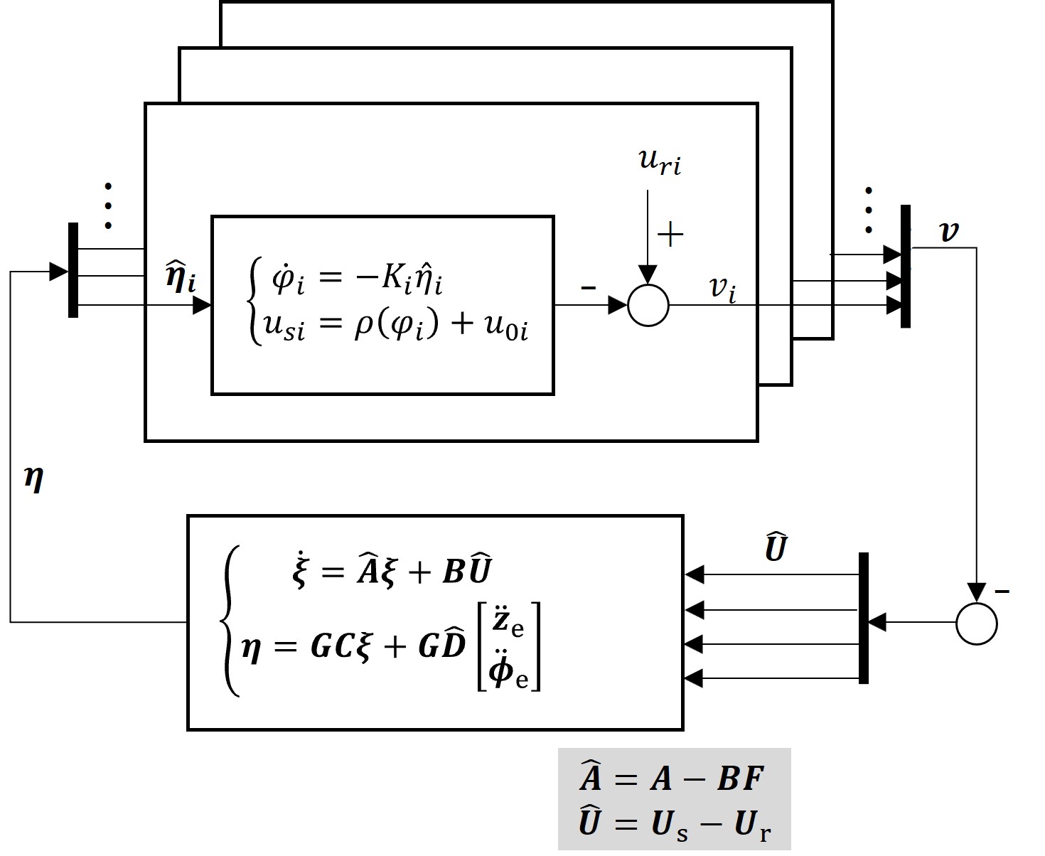
Figure 15: System

Furthermore, the entire system can be represented as Fig.15 using $v:=-U_{s}+U_{r}$. The difference from the system using the ASSC in the literature [2] is that it is extended from single output to multiple outputs and that an offset is added to the control input. For the offset, $v_{i}$ is expressed as follows:

$$\begin{split}v_{i}&=-u_{si}+u_{ri}=-\rho(\varphi_{i})-u_{0i}+u_{ri}\\ &=-\rho(\varphi_{i})-u_{0i}+(u_{0i}+d_{i})=-\rho(\varphi_{i})+d_{i}.\end{split}$$ (26)

$\rho(\varphi_{i})$ is used to compensate for the change $d_{i}$ from $u_{0i}$. Therefore, a storage function of eq.(24) is defined as follows:

$$V_{ci}:=\int_{0}^{\varphi_{i}}\frac{\rho(\varphi_{i})-\tilde{u}_{ri}(\varphi_{i})}{L_{i}(\varphi_{i})}d\varphi_{i}\geq 0,$$ (27)

where $L_{i}(\varphi_{i})$ is any constant satisfying $\underline{k}_{i}\leq L_{i}(\varphi_{i})\leq\bar{k}_{i}$. Moreover, if $d_{i}>0$, $\tilde{u}_{ri}(\varphi_{i})$ is defined as

$$\tilde{u}_{ri}(\varphi_{i}):=\left\{\begin{array}[]{l}d_{i}:\varphi_{i}\geq\rho^{-1}(d_{i})\\ \rho(\varphi_{i}):\varphi_{i}<\rho^{-1}(d_{i})\end{array}\right.,$$ (28)

and if $d_{i}\leq 0$, $\tilde{u}_{ri}(\varphi_{i})$ is defined as

$$\tilde{u}_{ri}(\varphi_{i}):=\left\{\begin{array}[]{l}d_{i}:\varphi_{i}\leq\rho^{-1}(d_{i})\\ \rho(\varphi_{i}):\varphi_{i}>\rho^{-1}(d_{i})\end{array}\right..$$ (29)

Then, the derivative of eq.(27) is as follows:

$$\begin{split}\dot{V}_{ci}&=\frac{\rho(\varphi_{i})-\tilde{u}_{ri}}{L_{i}(\varphi_{i})}\dot{\varphi}_{i}=-\tilde{K}_{i}(\rho(\varphi_{i})-\tilde{u}_{ri})\hat{\eta_{i}}\\ &=-\tilde{K}_{i}(\rho(\varphi_{i})-d_{i})\hat{\eta}_{i}-\tilde{K}_{i}(d_{i}-\tilde{u}_{ri}(\varphi_{i}))\hat{\eta}_{i}\\ &=-(\rho(\varphi_{i})-d_{i})\hat{\eta}_{i}-(\tilde{K}_{i}-1)(\rho(\varphi_{i})-d_{i})\hat{\eta}_{i}\\ &\hskip 14.22636pt-\tilde{K}_{i}(d_{i}-\tilde{u}_{ri}(\varphi_{i}))\hat{\eta}_{i}\\ &=-(\rho(\varphi_{i})-d_{i})\hat{\eta}_{i}-(\tilde{K}_{i}-1)\\ &\hskip 14.22636pt\left((\rho(\varphi_{i})-\tilde{u}_{ri}(\varphi_{i}))-(d_{i}-\tilde{u}_{ri}(\varphi_{i}))\right)\hat{\eta}_{i}\\ &\hskip 14.22636pt-\tilde{K}_{i}(d_{i}-\tilde{u}_{ri}(\varphi_{i}))\hat{\eta}_{i}\\ &=v_{i}\hat{\eta}_{i}-(\tilde{K}_{i}-1)(\rho(\varphi_{i})-\tilde{u}_{ri}(\varphi_{i}))\hat{\eta}_{i}\\ &\hskip 14.22636pt-(d_{i}-\tilde{u}_{ri}(\varphi_{i}))\hat{\eta}_{i}\end{split}$$ (30)

where $\tilde{K}_{i}:=K_{i}(\varphi_{i},\hat{\eta})/L_{i}(\varphi_{i})$. Moreover, $\tilde{u}_{r}$ is defined as

$$\tilde{u}_{r}:=\sum_{i=1}^{n}\tilde{u}_{ri}(\varphi_{i}).$$ (31)

Furthermore, an entire storage function is defined as

$$V_{c}:=\sum_{i=1}^{n}V_{ci}.$$ (32)

Thus, the derivative of eq.(32) is as follows:

$$\dot{V}_{c}:=v^{\top}\hat{\eta}-\sum_{i=1}^{n}(d_{i}-\tilde{u}_{ri}(\varphi_{i}))\hat{\eta}_{i}-\sum_{i=1}^{n}(\tilde{K}_{i}-1)(\rho(\varphi_{i})-\tilde{u}_{ri}(\varphi_{i}))\hat{\eta}_{i}.$$ (33)

Integrating eq.(33) over a time interval $[t_{0},t_{1}]$ yields

$$\begin{split}&V_{c}(t_{1})-V_{c}(t_{0})=\\ &\int_{t_{0}}^{t_{1}}v^{\top}\hat{\eta}dt-\int_{t_{0}}^{t_{1}}\sum_{i=1}^{n}(\tilde{K}_{i}-1)(\rho(\varphi_{i})-\tilde{u}_{ri}(\varphi_{i}))\hat{\eta}_{i}dt\\ &-\int_{t_{0}}^{t_{1}}\sum_{i=1}^{n}(d_{i}-\tilde{u}_{ri}(\varphi_{i}))\hat{\eta}_{i}dt.\end{split}$$ (34)

According to the definitions of $\tilde{K}_{i}$, $(\tilde{K}_{i}-1)$ is expressed as follows:

$$\varphi_{i}\hat{\eta}_{i}\leq 0\rightarrow(\tilde{K}_{i}-1)\leq 0$$ (35)

$$\varphi_{i}\hat{\eta}_{i}>0\rightarrow(\tilde{K}_{i}-1)\geq 0.$$ (36)

Furthermore, according to the definitions of $\tilde{u}_{ri}(\varphi_{i})$, if $\varphi_{i}\hat{\eta}_{i}\leq 0$,

$$\varphi_{i}>0,\hat{\eta}_{i}\leq 0\rightarrow(\rho(\varphi_{i})-\tilde{u}_{ri})\hat{\eta}_{i}\leq 0$$ (37)

$$\varphi_{i}\leq 0,\hat{\eta}_{i}>0\rightarrow(\rho(\varphi_{i})-\tilde{u}_{ri})\hat{\eta}_{i}\leq 0.$$ (38)

Moreover, if $\varphi_{i}\hat{\eta}_{i}>0$,

$$\varphi_{i}>0,\hat{\eta}_{i}>0\rightarrow(\rho(\varphi_{i})-\tilde{u}_{ri})\hat{\eta}_{i}\geq 0$$ (39)

$$\varphi_{i}\leq 0,\hat{\eta}_{i}\leq 0\rightarrow(\rho(\varphi_{i})-\tilde{u}_{ri})\hat{\eta}_{i}\geq 0.$$ (40)

Therefore, the second term of eq.(34) is as follows:

$$-\int_{t_{0}}^{t_{1}}\sum_{i=1}^{n}(\tilde{K}_{i}-1)(\rho(\varphi_{i})-\tilde{u}_{ri}(\varphi_{i}))\hat{\eta}_{i}dt\leq 0.$$ (41)

To investigate the third term of eq.(34), $V_{ui}$ is defined as

$$V_{ui}:=\int_{0}^{\varphi_{i}}(d_{i}-\tilde{u}_{ri}(\varphi_{i}))d\varphi_{i}\geq 0.$$ (42)

Moreover, the derivative of eq.(42) is as follows:

$$\dot{V}_{ui}=(d_{i}-\tilde{u}_{ri}(\varphi_{i}))\dot{\varphi_{i}}=-K_{i}(\varphi_{i},\hat{\eta}_{i})(d_{i}-\tilde{u}_{ri}(\varphi_{i}))\hat{\eta}_{i}.$$ (43)

Thus, we obtained the following.

$$\sum_{i=1}^{n}(d_{i}-\tilde{u}_{ri}(\varphi_{i}))\hat{\eta}_{i}=-\sum_{i=1}^{n}\left(\frac{1}{K_{i}(\varphi_{i},\hat{\eta}_{i})}\right)\dot{V}_{ui}.$$ (44)

Using eq.(44), the third term of eq.(34) can be expressed as follows:

$$-\int_{t_{0}}^{t_{1}}\sum_{i=1}^{n}(d_{i}-\tilde{u}_{ri}(\varphi_{i}))\hat{\eta}_{i}dt=\sum_{i=1}^{n}\int_{t_{0}}^{t_{1}}\left(\frac{1}{K_{i}(\varphi_{i},\hat{\eta}_{i})}\dot{V}_{ui}\right)dt$$ (45)

where $\dot{\bar{V}}_{ui}$ is introduced as follows:

$$\dot{\bar{V}}_{ui}:=\left\{\begin{array}[]{l}\dot{V}_{ui}:\dot{V}_{ui}\geq 0\\ 0:\dot{V}_{ui}<0\end{array}\right..$$ (46)

Using eq.(46), eq.(45) can be expressed as follows:

$$-\int_{t_{0}}^{t_{1}}\sum_{i=1}^{n}(d_{i}-\tilde{u}_{ri}(\varphi_{i}))\hat{\eta}_{i}dt\leq\sum_{i=1}^{n}k_{h}\int_{t_{0}}^{t_{1}}\dot{\bar{V}}_{ui}dt,\\$$ (47)

where $k_{h}$ is a positive constant that satisfies $0<1/K_{i}(\varphi_{i},\hat{\eta}_{i})\leq k_{h}$. Let the initial time be $\tau_{0}=t_{0}$, end time be $\tau_{T}=t_{1}$, interval time be $\tau_{i}\;(i=1,\dots,T-1)$, and number of discretized total times be $T$, eq.(47) can be expressed as follows:

$$\sum_{i=1}^{n}k_{h}\int_{t_{0}}^{t_{1}}\dot{\bar{V}}_{ui}dt$$ (48)

$$=\sum_{i=1}^{n}k_{h}(V_{ui}(\tau_{1})-V_{ui}(\tau_{0})+V_{ui}(\tau_{2})-V_{ui}(\tau_{1})+$$ (49)

$$\hskip 14.22636pt\dots+V_{ui}(\tau_{T})-V_{ui}(\tau_{T-1}))$$ (50)

$$=k_{h}\sum_{i=1}^{n}(V_{ui}(\tau_{T})-V_{ui}(\tau_{0})).$$ (51)

Furthermore, if $\varphi_{i}\geq\varphi_{\rm{p}i}$ and $\varphi_{i}<\varphi_{\rm{n}i}$, $d_{i}-\tilde{u}_{ri}(\varphi_{i})=0$. Thus, $V_{ui}$ can be expressed as follows:

$$V_{ui} =\int_{0}^{\varphi_{i}}(d_{i}-\tilde{u}_{ri}(\varphi_{i}))d\varphi_{i}$$ (52)

$$\leq\int_{0}^{\varphi_{i}}\Delta u_{\text{rm}}d\varphi_{i}=\Delta u_{\text{rm}}|\varphi_{i}|\leq\Delta u_{\text{rm}}\varphi_{\text{m}i}$$ (53)

where $\Delta u_{\text{rm}}:=\max_{\varphi_{i}}\rho(\varphi_{i})-\min_{\varphi_{i}}\rho(\varphi_{i})$ and $\varphi_{\text{m}i}:=\max\{|\varphi_{\rm{p}i}|,|\varphi_{\rm{n}i}|\}$. Therefore, using eq.(53), eq.(51) can be expressed as follows:

$$k_{h}\sum_{i=1}^{n}(V_{ui}(\tau_{T})-V_{ui}(\tau_{0}))\leq k_{h}n\Delta u_{\text{rm}}\varphi_{\text{m}i}.$$ (54)

Thus, we obtain the following:

$$-\int_{t_{0}}^{t_{1}}\sum_{i=1}^{n}(d_{i}-\tilde{u}_{ri}(\varphi_{i}))\hat{\eta}_{i}dt\leq C_{\text{u}},$$ (55)

where $C_{\text{u}}:=k_{h}n\Delta u_{\text{rm}}\varphi_{\text{m}i}$ satisfies $0\leq C_{\text{u}}\leq\infty$. Therefore, eq.(34) can be expressed as follows:

$$V_{c}(t_{1})-V_{c}(t_{0})\leq\int_{t_{0}}^{t_{1}}v^{\top}\hat{\eta}dt+C_{\text{u}}.$$ (56)

Suppose $V_{c}(t_{1})\geq 0$ and $C_{\text{u}}\geq 0$, then eq.(56) can be expressed as follows:

$$-C_{\text{V}}(t_{0})\leq\int_{t_{0}}^{t_{1}}v^{\top}\hat{\eta}dt,$$

where $C_{\text{V}}:=V_{c}(t_{0})+C_{\text{u}}$ satisfying $0\leq C_{\text{V}}(t_{0})\leq\infty$. Thus, according to [40], eq. (24) is passive.

Table 5: Rising time

Shape	Rectangle-shape				L-shaped
State	$X$	$Y$	$Z$	$\Psi$	$X$	$Y$	$Z$	$\Psi$
Our controller	$2.69$	$2.83$	$2.3$	$2.19$	$2.85$	$2.90$	$2.20$	$2.57$
PID controller	$2.76$	$2.99$	$2.13$	$2.21$	$2.85$	$2.89$	$2.05$	$2.33$

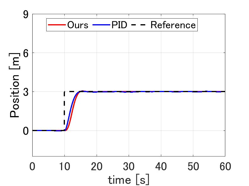
(a) Rectangle-shape $X$

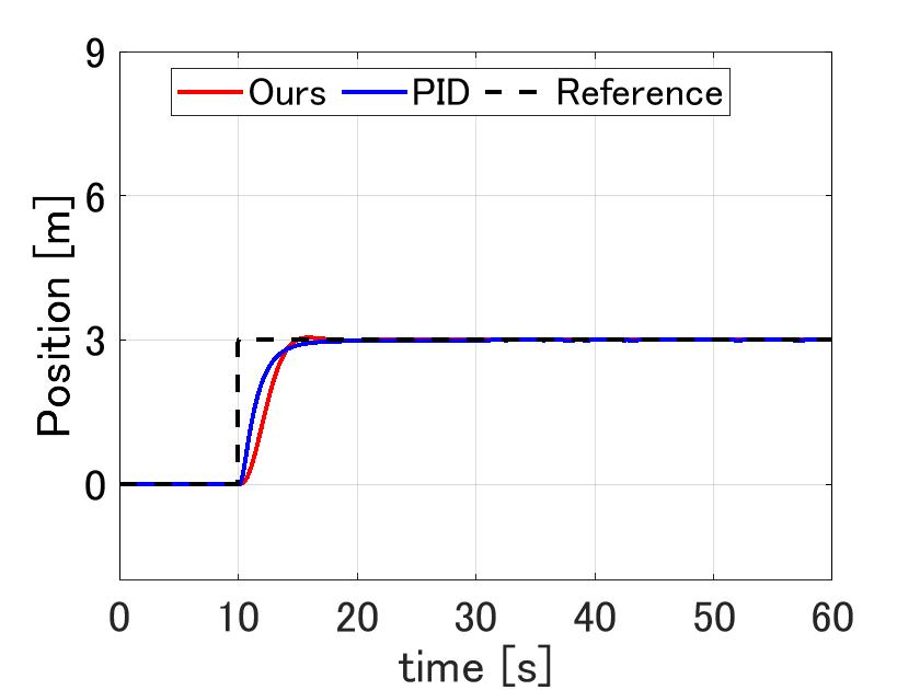
(b) Rectangle-shape $Y$

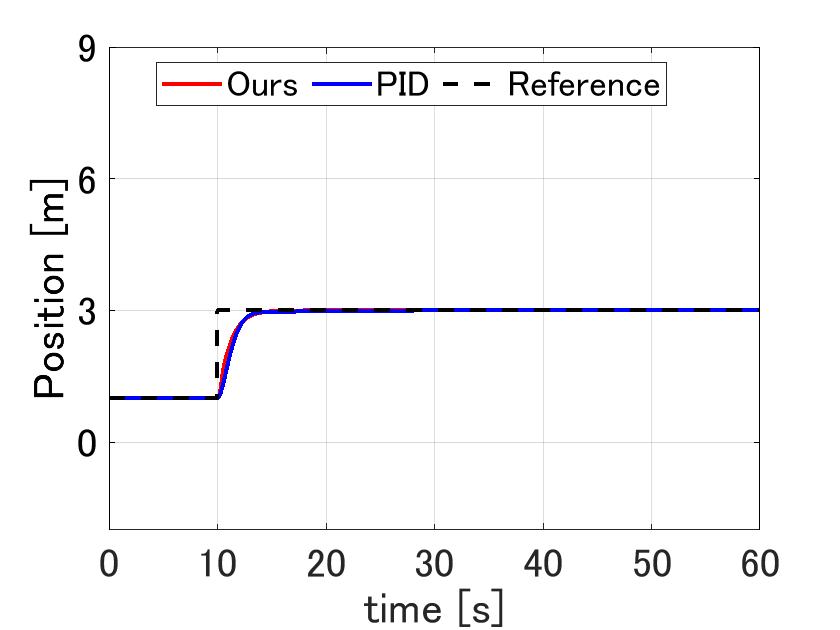
(c) Rectangle-shape $Z$

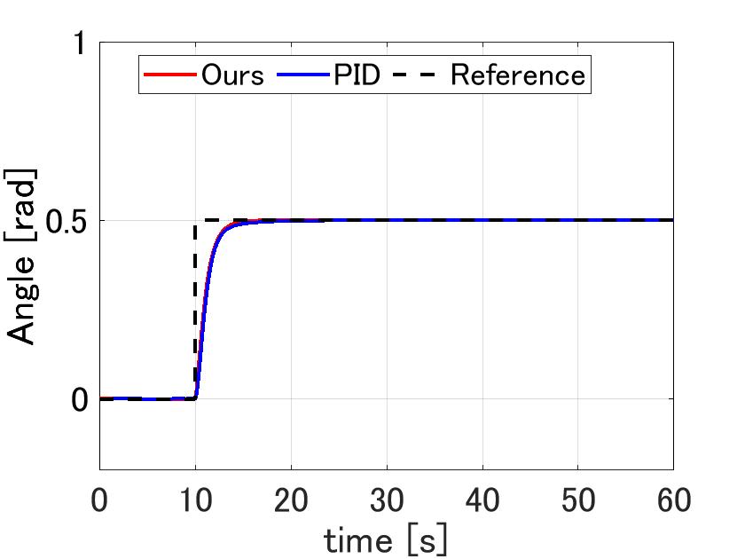
(d) Rectangle-shape $\psi$

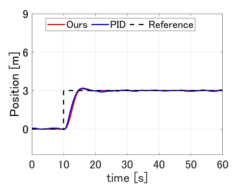
(e) L-shape $X$

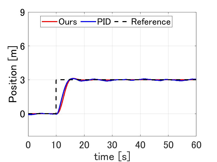
(f) L-shape $Y$

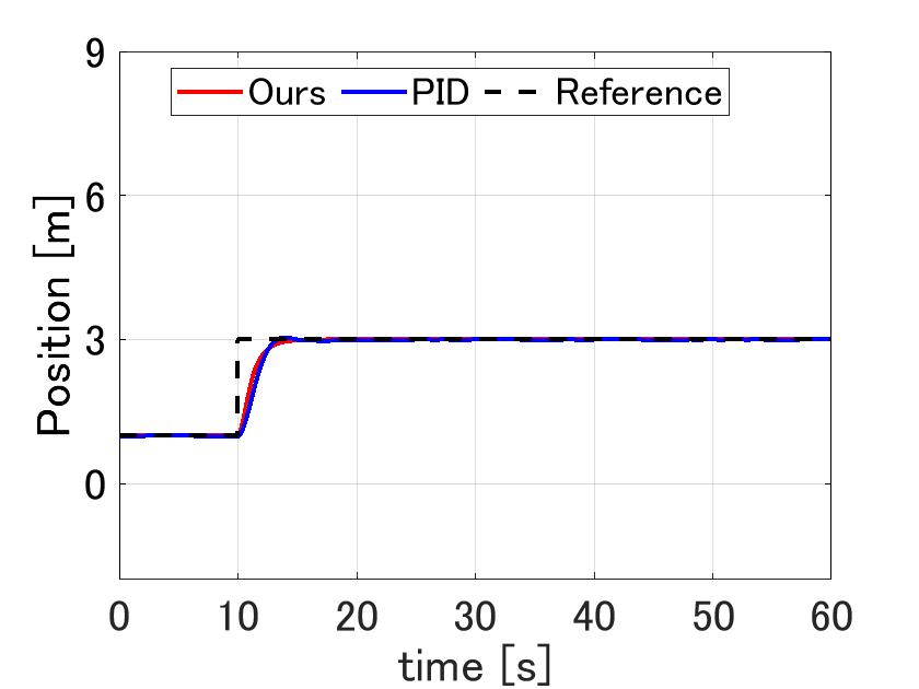
(g) L-shape $Z$

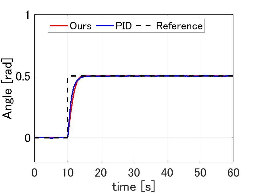
(h) L-shape $\psi$

Figure 16: Time series of the position, yaw angle, and reference of the Rectangular-shaped and L-shaped payloads using our controller (Ours) and PID controller (PID).

Appendix B PID controller

The parameters of the PID control, which is the comparison target of the proposed control, were designed to be the same as the rising time of the proposed control. Herein, the rising time is the time required for the response to increase from 10 % to 90 % of the way from the initial to the steady-state value. Each rising time is presented in Table 5, and a comparison of responses is shown in figure 16. We evaluated the step responses from $0$ to $3$ m for $X$ and $Y$, from $1$ to $3$ m for $Z$, and from $0$ rad to $0.5$ rad for $\psi$.

References

- [1] E. Ackerman and M. Koziol. The blood is here: Zipline’s medical delivery drones are changing the game in rwanda. IEEE Spectrum, 56:24–31, 2019.
- [2] Yasushi Amano, Tomohiko Jimbo, and Kenji Fujimoto. Tracking control for multi-agent systems using broadcast signals based on positive realness. arXiv preprint arXiv:2109.06372, 2021.
- [3] B. Anderson. A simplified viewpoint of hyperstability. IEEE Transactions on Automatic Control, 13:292–294, 1968.
- [4] Gustavo A Cardona, M Arevalo-Castiblanco, Duvan Tellez-Castro, J Calderon, and Eduardo Mojica-Nava. Robust adaptive synchronization of interconnected heterogeneous quadrotors transporting a cable-suspended load. In 2021 IEEE International Conference on Robotics and Automation (ICRA), pages 31–37. IEEE, 2021.
- [5] Ahmad Reza Cheraghi, Sahdia Shahzad, and Kalman Graffi. Past, present, and future of swarm robotics. In Intelligent Systems and Applications: Proceedings of the 2021 Intelligent Systems Conference (IntelliSys) Volume 3, pages 190–233. Springer, 2022.
- [6] Soon-Jo Chung, Aditya Avinash Paranjape, Philip Dames, Shaojie Shen, and Vijay Kumar. A survey on aerial swarm robotics. IEEE Transactions on Robotics, 34(4):837–855, 2018.
- [7] Micah Corah and Nathan Michael. Active estimation of mass properties for safe cooperative lifting. In 2017 IEEE International Conference on Robotics and Automation (ICRA), pages 4582–4587. IEEE, 2017.
- [8] Marco Dorigo, Dario Floreano, Luca Maria Gambardella, Francesco Mondada, Stefano Nolfi, Tarek Baaboura, Mauro Birattari, Michael Bonani, Manuele Brambilla, Arne Brutschy, et al. Swarmanoid: a novel concept for the study of heterogeneous robotic swarms. IEEE Robotics & Automation Magazine, 20(4):60–71, 2013.
- [9] V. Lippiello F. Ruggiero and A. Ollero. Aerial manipulation: A literature review. IEEE Robotics and Automation Letters, 3:1957–1964, 2018.
- [10] Joshua Fishman, Samuel Ubellacker, Nathan Hughes, and Luca Carlone. Dynamic grasping with a" soft" drone: From theory to practice. In 2021 IEEE/RSJ International Conference on Intelligent Robots and Systems (IROS), pages 4214–4221. IEEE, 2021.
- [11] Qimi Jiang and Vijay Kumar. The inverse kinematics of cooperative transport with multiple aerial robots. IEEE Transactions on Robotics, 29(1):136–145, 2012.
- [12] Hossein Bonyan Khamseh, Farrokh Janabi-Sharifi, and Abdelkader Abdessameud. Aerial manipulation—a literature survey. Robotics and Autonomous Systems, 107:221–235, 2018.
- [13] C Ronald Kube and Eric Bonabeau. Cooperative transport by ants and robots. Robotics and autonomous systems, 30(1-2):85–101, 2000.
- [14] Aishwarya Kumar, Puneet Kumar Gupta, and Ankita Srivastava. A review of modern technologies for tackling covid-19 pandemic. Diabetes & Metabolic Syndrome: Clinical Research & Reviews, 14(4):569–573, 2020.
- [15] Vijay Kumar and Nathan Michael. Opportunities and challenges with autonomous micro aerial vehicles. The International Journal of Robotics Research, 31(11):1279–1291, 2012.
- [16] Yoan D Landau. Adaptive control: The model reference approach. IEEE Transactions on Systems, Man, and Cybernetics, (1):169–170, 1984.
- [17] Nicola Lissandrini, Christos K Verginis, Pedro Roque, Angelo Cenedese, and Dimos V Dimarogonas. Decentralized nonlinear mpc for robust cooperative manipulation by heterogeneous aerial-ground robots. In 2020 IEEE/RSJ International Conference on Intelligent Robots and Systems (IROS), pages 1531–1536. IEEE, 2020.
- [18] Simone Martini, Davide Di Baccio, Francisco Alarcón Romero, Antidio Viguria Jiménez, Lucia Pallottino, Gianluca Dini, and Aníbal Ollero. Distributed motion misbehavior detection in teams of heterogeneous aerial robots. Robotics and Autonomous Systems, 74:30–39, 2015.
- [19] Lorenz Meier, Petri Tanskanen, Friedrich Fraundorfer, and Marc Pollefeys. Pixhawk: A system for autonomous flight using onboard computer vision. In 2011 IEEE International Conference on Robotics and Automation, pages 2992–2997. IEEE, 2011.
- [20] Daniel Mellinger, Michael Shomin, Nathan Michael, and Vijay Kumar. Cooperative grasping and transport using multiple quadrotors. In Distributed autonomous robotic systems, pages 545–558. Springer, 2013.
- [21] Jiawei Meng, Joao Buzzatto, Yuanchang Liu, and Minas Liarokapis. On aerial robots with grasping and perching capabilities: A comprehensive review. Frontiers in Robotics and AI, page 405, 2022.
- [22] Nathan Michael, Jonathan Fink, and Vijay Kumar. Cooperative manipulation and transportation with aerial robots. Autonomous Robots, 30(1):73–86, 2011.
- [23] Diego González Morín, José Araujo, Soma Tayamon, and Lars AA Andersson. Autonomous cooperative flight of rigidly attached quadcopters. In 2019 International Conference on Robotics and Automation (ICRA), pages 5309–5315. IEEE, 2019.
- [24] Bingguo Mu and Pakpong Chirarattananon. Universal flying objects: Modular multirotor system for flight of rigid objects. IEEE Transactions on Robotics, 36(2):458–471, 2019.
- [25] Koshi Oishi, Yasushi Amano, and Tomohiko Jimbo. Cooperative transportation with multiple aerial robots and decentralized control for unknown payloads. arXiv preprint arXiv:2111.01963, 2021.
- [26] Koshi Oishi and Tomohiko Jimbo. Autonomous cooperative transportation system involving multi-aerial robots with variable attachment mechanism. In 2021 IEEE/RSJ International Conference on Intelligent Robots and Systems (IROS), pages 6322–6328. IEEE, 2021.
- [27] Anibal Ollero, Guillermo Heredia, Antonio Franchi, Gianluca Antonelli, Konstantin Kondak, Alberto Sanfeliu, Antidio Viguria, J Ramiro Martinez-de Dios, Francesco Pierri, Juan Cortés, et al. The aeroarms project: Aerial robots with advanced manipulation capabilities for inspection and maintenance. IEEE Robotics & Automation Magazine, 25(4):12–23, 2018.
- [28] Raymond Oung and Raffaello D’Andrea. The distributed flight array. Mechatronics, 21(6):908–917, 2011.
- [29] Pedro O Pereira and Dimos V Dimarogonas. Pose stabilization of a bar tethered to two aerial vehicles. Automatica, 112:108695, 2020.
- [30] Pedro O Pereira, Pedro Roque, and Dimos V Dimarogonas. Asymmetric collaborative bar stabilization tethered to two heterogeneous aerial vehicles. In 2018 IEEE International Conference on Robotics and Automation (ICRA), pages 5247–5253. IEEE, 2018.
- [31] Fatemeh Rekabi, Farzad A Shirazi, Mohammad Jafar Sadigh, and Mahmood Saadat. Distributed output feedback nonlinear h formation control algorithm for heterogeneous aerial robotic teams. Robotics and Autonomous Systems, 136:103689, 2021.
- [32] Wei Ren and Nathan Sorensen. Distributed coordination architecture for multi-robot formation control. Robotics and Autonomous Systems, 56(4):324–333, 2008.
- [33] Yara Rizk, Mariette Awad, and Edward W Tunstel. Cooperative heterogeneous multi-robot systems: A survey. ACM Computing Surveys (CSUR), 52(2):1–31, 2019.
- [34] Sujan Sarker, Lafifa Jamal, Syeda Faiza Ahmed, and Niloy Irtisam. Robotics and artificial intelligence in healthcare during covid-19 pandemic: A systematic review. Robotics and autonomous systems, 146:103902, 2021.
- [35] Philipp Schillinger, Sergio García, Alexandros Makris, Konstantinos Roditakis, Michalis Logothetis, Konstantinos Alevizos, Wei Ren, Pouria Tajvar, Patrizio Pelliccione, Antonis Argyros, et al. Adaptive heterogeneous multi-robot collaboration from formal task specifications. Robotics and Autonomous Systems, 145:103866, 2021.
- [36] Kazuki Shibata, Tomohiko Jimbo, and Takamitsu Matsubara. Deep reinforcement learning of event-triggered communication and control for multi-agent cooperative transport. In 2021 IEEE International Conference on Robotics and Automation (ICRA), pages 8671–8677. IEEE, 2021.
- [37] Kazuki Shibata, Tomohiko Jimbo, and Takamitsu Matsubara. Deep reinforcement learning of event-triggered communication and consensus-based control for distributed cooperative transport. Robotics and Autonomous Systems, 159:104307, 2023.
- [38] Behzad Shirani, Majdeddin Najafi, and Iman Izadi. Cooperative load transportation using multiple uavs. Aerospace Science and Technology, 84:158–169, 2019.
- [39] Sphero. Sphero sprk+ robot ball | educational robot toy | sphero. https://sphero.com/collections/all/family_sprk, Access in 2023.
- [40] A. van der Schaft. L2-gain and passivity techniques in nonlinear control, volume 218. Springer, Berlin, Heidelberg, 2000.
- [41] Daniel KD Villa, Alexandre S Brandao, and Mário Sarcinelli-Filho. A survey on load transportation using multirotor uavs. Journal of Intelligent & Robotic Systems, 98(2):267–296, 2020.
- [42] Hanlei Wang. Passivity based synchronization for networked robotic systems with uncertain kinematics and dynamics. Automatica, 49(3):755–761, 2013.
- [43] Zijian Wang, Sumeet Singh, Marco Pavone, and Mac Schwager. Cooperative object transport in 3d with multiple quadrotors using no peer communication. In 2018 IEEE International Conference on Robotics and Automation (ICRA), pages 1064–1071. IEEE, 2018.
- [44] Christian Wankmüller, Maximilian Kunovjanek, and Sebastian Mayrgündter. Drones in emergency response–evidence from cross-border, multi-disciplinary usability tests. International Journal of Disaster Risk Reduction, 65:102567, 2021.
- [45] Lin Zhang, Yufeng Sun, Andrew Barth, and Ou Ma. Decentralized control of multi-robot system in cooperative object transportation using deep reinforcement learning. IEEE Access, 8:184109–184119, 2020.