Curvature-enhanced multipartite coherence in the multiverse

Abstract

Here, we study quantum coherence of N-partite GHZ (Greenberger-Horne-Zeilinger) and W states in the multiverse consisting of $N$ causally disconnected de Sitter spaces. Interestingly, N-partite coherence increases monotonically as the curvature increases, while the Unruh effect destroys multipartite coherence in Rindler spacetime. Conversely, the curvature effect destroys quantum entanglement and discord, meaning that the curvature effect is beneficial to quantum coherence and harmful to quantum correlations in the multiverse. We find that, with the increase of $n$ expanding de Sitter spaces, N-partite coherence of GHZ state increases monotonically for any curvature, while quantum coherence of the W state decreases or increases monotonically depending on the curvature. We find a distribution relationship, which indicates that the correlated coherence of N-partite W state is equal to the sum of all bipartite correlated coherence in the multiverse. Multipartite coherence exhibits unique properties in the multiverse, which argues that it may provide some evidence for the existence of the multiverse.

I Introduction

Quantum coherence, arising from the superposition principle of quantum state, is one of the important features of the quantum world, and is the basis of the fundamental phenomena of quantum interference L1 . Like quantum entanglement, quantum coherence is an important quantum resource, which can be applied in quantum information processing, solid state physics, quantum optics, nanoscale thermodynamics, and biological systems L2 ; L3 ; L4 ; L5 ; L6 ; L7 ; L8 ; L9 ; L10 ; L11 ; L12 . Although quantum coherence is of great importance, it did not attract more attention until Baumgratz $et$ $al$. proposed a rigorous resource theory framework for the quantization of coherence, such as the $l_{1}$ norm of coherence and the relative entropy of coherence L13 . For complex multipartite systems, the $l_{1}$ norm of coherence is more directly calculated and is easier to obtain analytical expression than the relative entropy of coherence. On the other hand, as the quantum information task becomes more and more complex, we need to deal with it with multipartite coherence.

Observer-dependent quantum entanglement can be discussed in the background of an expanding universe L14 ; L15 ; L16 ; L17 . The theory of inflationary cosmology and our current observations suggest that our universe may approach the de Sitter space with a positive cosmological constant in the far past and the far future, which is the unique maximally symmetric curved spacetime. Any two mutually separated $R$ and $L$ regions eventually are causally disconnected in de Sitter space L18 , where the universe expands exponentially. This is most appropriately described by spanning open universe coordinates for two open charts in de Sitter space. The positive frequency mode functions of a free massive scalar field correspond to the Bunch-Davies vacuum (the Euclidean vacuum) that supports on both $R$ and $L$ regions. Using them, entanglement entropy between two causally disconnected regions in de Sitter space has been studied in the Bunch-Davies vacuum and $\alpha$-vacua L19 ; L20 ; L21 ; L22 ; L23 ; L24 . Motivated by the work, quantum steering, entanglement and discord were also studied L25 ; L26 ; L27 ; L28 . Since it was shown that quantum entanglement between causally separated regions (beyond the size of the Hubble horizon) exists in de Sitter space, there may be the observable effects of quantum correlations on the cosmic microwave background (CMB) in our expanding universe.

The vacuum fluctuations in our expanding universe may be entangled with those in another part of the multiverse L19 . In fact, quantum entanglement of the reduced density matrix influences the shape of the spectrum on large scales, which is comparable to or greater than the curvature radius L20 . This could be the observational signature of the multiverse. In addition, quantum coherence may be determined by the observers in the process of bubble nucleation. It is well known that quantum coherence reflects the nonclassical world better than quantum entanglement, which is considered to be derived from the nonlocal superposition principle of quantum state. In other words, quantum entanglement is a special kind of quantum coherence (genuine coherence) L30 ; L31 ; L32 . In general, quantum entanglement and coherence show similar properties in a relativistic setting. It is not clear whether multipartite coherence and quantum entanglement have similar properties in the multiverse. Therefore, demonstrating the observer’s dependence on multipartite coherence in the multiverse is one of the motivations for our work.

Another motivation for our work is better to understand the multiverse through multipartite coherence. According to the string landscape and inflationary cosmology, our universe may not be the just one, but part of the multiverse L33 ; L34 ; L35 ; L36 ; L37 . In the structure of the multiverse model, there may be many causally disconnected de Sitter bubbles (de Sitter universes). Until recently, the multiverse is merely a philosophical conjecture that has so far been untestable. However, in the multiverse, quantum coherence between $N$ causally separated universes may generate detectable signatures. Some of their quantum states that are far from the Bunch-Davies vacuum may be entangled with another universes L19 . Then, we introduce $N$ observers who determine quantum coherence between $N$ causally disconnected de Sitter spaces. We assume $n$ observers inside de Sitter universes and want to see how the inside $n$ observers detect the signature of quantum coherence with another $N-n$ de Sitter universes.

In this paper, we discuss quantum coherence of N-partite GHZ and W states of massive scalar fields in de Sitter universes. We assume that $N-n$ observers are in their respective static universes, while $n$ observers are in their expanding universes. Here an observer corresponds to a universe. We calculate N-partite coherence and obtain its analytical expression in de Sitter background. We find that, with the increase of the curvature, N-partite coherence increases monotonically, while quantum correlation decreases monotonically as the curvature increases in de Sitter universes L25 ; L26 ; L27 ; L28 . It is important to note that quantum correlation and coherence decrease with the increase of the acceleration in Rindler spacetime L38 ; L39 ; ZL1 ; ZL2 ; ZL3 ; ZL4 . This indicates that quantum correlation and coherence exhibit opposite behaviors in the multiverse and show similar properties in Rindler spacetime. Therefore, we can gain a deeper understanding of the multiverse from the perspective of quantum resources. Although this research may involve quantities that cannot be directly detected in the multiverse, it provides profound insights into the fundamental nature of quantum systems in different spacetime backgrounds. In addition, quantum coherence can be observed experimentally FGH1 ; FGH2 . We believe that understanding the behavior of quantum coherence can provide guidance for simulating multiverse using quantum systems ZQQL1 ; ZQQL2 ; ZQQL3 .

Interestingly, quantum coherence of N-partite GHZ state in de Sitter universes has nonlocal coherence and local coherence that can exist in subsystems, while quantum coherence of N-partite GHZ state in Rindler spacetime is genuinely global that cannot exist in any subsystems. We quantify the nonlocal coherence in terms of correlated coherence of the multipartite systems in the multiverse L30 ; L31 ; L32 . Unlike N-partite coherence of W state in Rindler spacetime L38 ; L39 , N-partite coherence of W state in de Sitter universes is not monogamous. However, the correlated coherence of N-partite W state is equal to the sum of the correlated coherence of all the bipartite subsystems in de Sitter universes. With the increase of the $n$, quantum coherence of W state decreases or increases monotonically depending on curvature, while N-partite coherence of GHZ state increases monotonically for any curvature. These results show some unique phenomena of multipartite coherence in de Sitter universes, which provides the possibility for us to find the multiverse.

The paper is organized as follows. In Sec. II, we briefly introduce the quantization of the free massive scalar field in de Sitter space. In Sec. III, we study quantum coherence of tripartite GHZ and W states in the multiverse. In Sec. IV, we extend the relevant research to the N-partite systems. The last section is devoted to a brief conclusion.

II Quantization of scalar field in de Sitter space

We consider a free scalar field $\phi$ with the mass $m$ in the Bunch-Davies vacuum of de Sitter space represented by metric $g_{\mu\nu}$. The action of the field is given by

$$S=\int d^{4}x\sqrt{-g}\left[\,-\frac{1}{2}\,g^{\mu\nu}\partial_{\mu}\phi\,\partial_{\nu}\phi-\frac{m^{2}}{2}\phi^{2}\,\right]\,.$$ (1)

The coordinate systems of the open chart in de Sitter space can be obtained by analytic continuation from the Euclidean metric and divided into two parts that we call the $R,L$. The $R$ and $L$ regions, which are covered, respectively, by the coordinates $(t_{L},r_{L})$ and $(t_{R},r_{R})$ in de Sitter space, are causally disconnected, and their metrics are given, respectively, by

$$ds^{2}_{R} = H^{-2}\left[-dt^{2}_{R}+\sinh^{2}t_{R}\left(dr^{2}_{R}+\sinh^{2}r_{R}\,d\Omega^{2}\right)\right]\,,$$

$$ds^{2}_{L} = H^{-2}\left[-dt^{2}_{L}+\sinh^{2}t_{L}\left(dr^{2}_{L}+\sinh^{2}r_{L}\,d\Omega^{2}\right)\right]\,,$$ (2)

where $H^{-1}$ is the Hubble radius and $d\Omega^{2}$ is the metric on the two-sphere L40 . In order to obtain the analytic continuation solutions in the $R$ or $L$ regions, we need to resolve this process in the Euclidean hemisphere. It is natural to choose the Euclidean vacuum ( Bunch-Davies vacuum) with de Sitter invariance as the initial condition. Therefore, it is necessary to find the positive frequency mode functions corresponding to the Euclidean vacuum. By separating the variables, we get

$$\phi=\frac{H}{\sinh t}\chi_{p}(t)Y_{p\ell m}(r,\Omega),$$ (3)

and the solutions of the Klein-Gordon equations for $\chi_{p}(t)$ and $Y_{p\ell m}(r,\Omega)$ in the $R$ or $L$ regions are found to be

$$\bigg{[}\frac{\partial^{2}}{\partial t^{2}}+3\coth t\frac{\partial}{\partial t}+\frac{1+p^{2}}{\sinh^{2}t}+\frac{m^{2}}{H^{2}}\bigg{]}\chi_{p}(t)=0,$$ (4)

$$\bigg{[}\frac{\partial^{2}}{\partial r^{2}}+2\coth t\frac{\partial}{\partial r}-\frac{1}{\sinh^{2}t}\mathbf{L^{2}}\bigg{]}Y_{p\ell m}(r,\Omega)=-(1+p^{2})Y_{p\ell m}(r,\Omega),$$ (5)

where $Y_{p\ell m}(r,\Omega)$ are eigenfunctions on the three-dimensional hyperboloid, and the $\mathbf{L^{2}}$ is the Laplacian operator on the unit two-sphere L19 .

The positive frequency mode functions corresponding to the Euclidean vacuum that is supported both on the $R$ and $L$ regions are given by

$$\chi_{p,\sigma}(t)=\left\{\begin{array}[]{l}\frac{e^{\pi p}-i\sigma e^{-i\pi\nu}}{\Gamma(\nu+ip+\frac{1}{2})}P_{\nu-\frac{1}{2}}^{ip}(\cosh t_{R})-\frac{e^{-\pi p}-i\sigma e^{-i\pi\nu}}{\Gamma(\nu-ip+\frac{1}{2})}P_{\nu-\frac{1}{2}}^{-ip}(\cosh t_{R})\,,\\ \\ \frac{\sigma e^{\pi p}-i\,e^{-i\pi\nu}}{\Gamma(\nu+ip+\frac{1}{2})}P_{\nu-\frac{1}{2}}^{ip}(\cosh t_{L})-\frac{\sigma e^{-\pi p}-i\,e^{-i\pi\nu}}{\Gamma(\nu-ip+\frac{1}{2})}P_{\nu-\frac{1}{2}}^{-ip}(\cosh t_{L})\,,\end{array}\right.$$ (9)

where $P^{\pm ip}_{\nu-\frac{1}{2}}$ are the associated Legendre functions and $\sigma=\pm 1$ is used for distinguishing the independent solutions in each open region. The normalization factor for these solutions is given by $N_{p}=\frac{4\sinh\pi p\,\sqrt{\cosh\pi p-\sigma\sin\pi\nu}}{\sqrt{\pi}\,|\Gamma(\nu+ip+\frac{1}{2})|}\,.$ In the above solutions, $\nu$ is a mass parameter that is given by

$$\nu=\sqrt{\frac{9}{4}-\frac{m^{2}}{H^{2}}}\,.$$ (10)

Note that the two special values of the mass parameters $\nu=1/2$ and $\nu=3/2$ correspond to the conformally coupled massless scalar and the minimally coupled massless limit, respectively. In order to simplify our discussion, we take $p$ as the curvature parameter of de Sitter space, and the influence of curvature gets stronger when $p$ is less than $1$. The scalar field can be expanded in terms of the annihilation and creation operators

$$\hat{\phi}(t,r,\Omega)=\frac{H}{\sinh t}\int dp\sum_{\sigma,\ell,m}\left[\,a_{\sigma p\ell m}\,\chi_{p,\sigma}(t)+a_{\sigma p\ell-m}^{\dagger}\,\chi^{*}_{p,\sigma}(t)\right]Y_{p\ell m}(r,\Omega)\,,$$ (11)

where $a_{\sigma p\ell m}$ satisfies $a_{\sigma p\ell m}|0\rangle_{\rm BD}=0$ in the Bunch-Davies vacuum. We introduce a Fourier mode field operator

$$\phi_{p\ell m}(t)\equiv\sum_{\sigma}\left[\,a_{\sigma p\ell m}\,\chi_{p,\sigma}(t)+a_{\sigma p\ell-m}^{\dagger}\,\chi^{*}_{p,\sigma}(t)\right]\,.$$ (12)

For simplicity, hereafter we omit the indices $p$, $\ell$, $m$ in the operators $\phi_{p\ell m}$, $a_{\sigma p\ell m}$ and $a_{\sigma p\ell-m}^{\dagger}$. For example, the mode functions and the associated Legendre functions can be rewritten as $P_{\nu-1/2}^{ip}(\cosh t_{R,L})\rightarrow P^{R,L}$, $P_{\nu-1/2}^{-ip}(\cosh t_{R,L})\rightarrow P^{R*,L*}$ and $\chi_{p,\sigma}(t)\rightarrow\chi^{\sigma}$.

Additionally, we can consider another positive frequency mode function for $R$ or $L$ vacuum that has support only on the $R$ or $L$ region, respectively. They are given by

$$\varphi^{q}=\left\{\begin{array}[]{ll}\frac{|\Gamma(1+ip)|}{\sqrt{2p}}P^{q}{}&\mbox{in region}~{}q\,,\\ 0{}&\mbox{in the opposite region}\,,\end{array}\right.$$ (15)

where $q=(R,L)$. Then we introduce the new annihilation and creation operators ($b_{q},b_{q}^{\dagger}$) that satisfy $b_{q}|0\rangle_{q}=0$ in different regions. Because the Fourier mode field operator is the same under the change of mode functions, we can relate the annihilation and creation operators ($b_{q},b_{q}^{\dagger}$) and $(a_{\sigma},a_{\sigma}^{\dagger})$ in different reference L19 . Therefore, we have

$$\phi(t)=a_{\sigma}\,\chi^{\sigma}+a_{\sigma}^{\dagger}\,\chi^{\sigma}{}^{*}=b_{q}\,\varphi^{q}+b_{q}^{\dagger}\,\varphi^{q}{}^{*}\,.$$ (16)

Using the Bogoliubov transformation between the operators, the Bunch-Davies vacuum and single particle excitation states can be constructed from the states in $R$ and $L$ regions L28 , which can be expressed as

$$|0\rangle_{\rm BD}=\sqrt{1-|\gamma_{p}|^{2}}\sum_{n=0}^{\infty}\gamma_{p}^{n}|n\rangle_{L}|n\rangle_{R}\,,$$ (17)

$$|1\rangle_{\rm BD}=\frac{1-|\gamma_{p}|^{2}}{\sqrt{2}}\sum_{n=0}^{\infty}\gamma^{n}_{p}\sqrt{n+1}\big{[}|(n+1)\rangle_{\rm L}|n\rangle_{\rm R}+|n\rangle_{\rm L}|(n+1)\rangle_{\rm R}\big{]},$$ (18)

where $|n\rangle_{R}$ and $|n\rangle_{L}$ correspond to the two modes of the $R$ and $L$ de Sitter open charts, respectively, and the parameter $\gamma_{p}$ reads

$$\gamma_{p}=i\frac{\sqrt{2}}{\sqrt{\cosh 2\pi p+\cos 2\pi\nu}+\sqrt{\cosh 2\pi p+\cos 2\pi\nu+2}}\,.$$ (19)

Now, we elaborate on the assertion that $p$ can be regarded as the curvature parameter of the de Sitter space. Employing Eq.(17), the reduced density matrix from the Bunch-Davies basis to the basis of the open chart in the $L$ region can be expressed as

$$\rho_{\rm L}=\rm{Tr_{R}(|0\rangle_{BD}\langle 0|)}=(1-|\gamma_{p}|^{2})\sum_{n=0}^{\infty}|\gamma_{p}|^{2n}|n\rangle_{\rm L}\langle n|.$$ (20)

Similarly, we can also obtain the reduced density matrix from the Minkowski basis to the Rindler basis that is found to be

$$\rho_{\rm I}=(1-e^{-2\pi\frac{\omega}{a}})\sum_{n=0}^{\infty}e^{-2\pi n\frac{\omega}{a}}|n\rangle_{\rm I}\langle n|,$$ (21)

where $a$ is the acceleration ZL1 ; ZL3 . From Eq.(20) and Eq.(21), we can obtain $a=-\pi\omega/\ln|\gamma_{p}|$. For the given values of $\nu$ and $\omega$, it is evident that the temperature $T_{U}=\frac{a}{2\pi}$ is a monotonically decreasing function of $p$. For $\nu=1/2$ and masslessness $\nu=3/2$, we obtain $|\gamma_{p}|=e^{-\pi p}$ and then the reduced density matrix can be expressed as

$$\rho_{\rm L}=(1-e^{-2\pi p})\sum_{n=0}^{\infty}e^{-2\pi pn}|n\rangle_{\rm L}\langle n|.$$ (22)

The resulting Eq.(22) is a thermal state with the temperature

$$T=\frac{H}{2\pi}.$$ (23)

We can find that $H$ is a monotonic decreasing function of $p$. In this context, we assert that $p$ serves as a descriptor for the curvature of de Sitter space; specifically, the smaller the $p$, the larger the curvature. This assertion has been utilized previously L25 ; L26 ; L27 ; L28 .

III Tripartite coherence of scalar fields in the multiverse

Utilizing this Bogoliubov transformation given by Eqs.(17) and (18), we discover that the initial state of the Bunch-Davies mode observed by an observer in the global chart corresponds to a two-mode squeezed state in the open charts. These two modes correspond to the fields observed in the $R$ and $L$ charts. If we exclusively examine one of the open charts, let’s say $L$, we cannot access to the modes in the causally disconnected $R$ region and must consequently trace over the inaccessible region. This situation is analogous to the relationship between an observer in a Minkowski chart and another in one of the two Rindler charts. In this sense, the global chart and Minkowski chart encompass the entire spacetime geometry, while the open charts and Rindler charts cover only a portion of the spacetime. From the above analysis, we find that the time evolution does not play a direct role in the calculations presented in the paper. The focus is primarily on the initial quantum states and the subsequent tracing out of parts of the density matrix.

In the structure of the multiverse model, there may be many causally disconnected de Sitter bubbles (de Sitter universes), and the inside of a nucleated bubble looks like an open universe. Along this line, we initially consider two typical tripartite states-GHZ and W states shared by Alice, Bob, and Charlie who determine quantum coherence between three causally disconnected de Sitter spaces. The technology for preparing GHZ and W states in experiments has become very mature plm1 ; plm2 . By removing a single particle from the W state, the ensuing bipartite state remains entangled. Thus, the W state demonstrates a remarkable persistence of quantum entanglement in the face of particle loss. Unlike W state, quantum entanglement and coherence of GHZ state only exist in three particles. Then, we set Bob and Charlie, respectively, to stay in the $L$ regions of two expanded de Sitter universes, and Alice is in the global chart of the other de Sitter space without expansion. If we probe only an open chart, such as $L$, the observer cannot access the mode in the causally disconnected $R$ region, and the inaccessible $R$ region must be traced over. In other words, in composite quantum systems, we only focus on the modes under consideration, so we need to trace the remaining modes. Then a pure state of the observers is going to be a mixed state. Therefore, thermal noise introduced by the expanding universe destroys quantum correlations L25 ; L26 ; L27 ; L28 . In the following, we will explore the properties of tripartite coherence in the multiverse.

III.1 Tripartite GHZ state

We assume that three observers, Alice, Bob, and Charlie share a tripartite GHZ state of the free massive scalar field defined as

$$|GHZ\rangle_{ABC}=\frac{1}{\sqrt{2}}[|0\rangle_{A,\rm BD_{1}}|0\rangle_{B,\rm BD_{2}}|0\rangle_{C,\rm BD_{3}}+|1\rangle_{A,\rm BD_{1}}|1\rangle_{B,\rm BD_{2}}|1\rangle_{C,\rm BD_{3}}].$$ (24)

Here, Alice, Bob, and Charlie are in the three causally disconnected de Sitter spaces $(\rm BD_{1})$, $(\rm BD_{2})$ and $(\rm BD_{3})$, respectively. Then, we consider that Bob and Charlie are in the $L$ regions of expanded de Sitter universes and Charlie is in a global chart of the other de Sitter space. For convenience, we omit the subscript $\rm{BD}$. Using Eqs.(17) and (18), we can rewrite Eq.(24) as

$$\begin{aligned} |GHZ\rangle_{AB\bar{B}C\bar{C}}=&\frac{1-|\gamma_{p}|^{2}}{\sqrt{2}}\sum_{n,m=0}^{\infty}\gamma^{n}_{p}\gamma^{m}_{p}\bigg{[}|0\rangle_{A}|n\rangle_{B}|n\rangle_{\bar{B}}|m\rangle_{C}|m\rangle_{\bar{C}}\\ +&\frac{1-|\gamma_{p}|^{2}}{2}\sqrt{n+1}\sqrt{m+1}|1\rangle_{A}(|n+1\rangle_{B}|n\rangle_{\bar{B}}+|n\rangle_{B}|n+1\rangle_{\bar{B}})\\ \otimes&(|m+1\rangle_{C}|m\rangle_{\bar{C}}+|m\rangle_{C}|m+1\rangle_{\bar{C}})\bigg{]},\end{aligned}$$ (25)

where the modes $\bar{B}$ and $\bar{C}$ are in the $R$ regions. Since the $R$ and $L$ regions are causally disconnected, we need to trace over the modes $\bar{B}$ and $\bar{C}$ in the $R$ regions and obtain the reduced density matrix as

$$\rho_{ABC}=\frac{(1-|\gamma_{p}|^{2})^{2}}{2}\sum_{n,m=0}^{\infty}\gamma_{p}^{2n}\gamma_{p}^{2m}\rho_{n,m},$$ (26)

where

$$\rho_{n,m}= |0\rangle_{A}\langle 0||n\rangle_{B}\langle n||m\rangle_{C}\langle m|+\frac{1-|\gamma_{p}|^{2}}{2}\sqrt{n+1}\sqrt{m+1}|0\rangle_{A}\langle 1|$$ (27)

$$\otimes (|n\rangle_{B}\langle n+1|+\gamma_{p}|n+1\rangle_{B}\langle n|)(|m\rangle_{C}\langle m+1|+\gamma_{p}|m+1\rangle_{C}\langle m|)$$

$$+ \frac{1-|\gamma_{p}|^{2}}{2}\sqrt{n+1}\sqrt{m+1}|1\rangle_{A}\langle 0|(|n+1\rangle_{B}\langle n|+\gamma_{p}^{*}|n\rangle_{B}\langle n+1|)$$

$$\otimes (|m+1\rangle_{C}\langle m|+\gamma_{p}^{*}|m\rangle_{C}\langle m+1|)+\frac{(1-|\gamma_{p}|^{2})^{2}}{4}|1\rangle_{A}\langle 1|$$

$$\otimes [(n+1)(|n+1\rangle_{B}\langle n+1|+|n\rangle_{B}\langle n|)+\sqrt{n+2}\sqrt{n+1}$$

$$\times (\gamma_{p}|n+2\rangle_{B}\langle n|+\gamma_{p}^{*}|n\rangle_{B}\langle n+2|)][(m+1)(|m+1\rangle_{C}\langle m+1|+|m\rangle_{C}\langle m|)$$

$$+ \sqrt{m+2}\sqrt{m+1}(\gamma_{p}|m+2\rangle_{C}\langle m|+\gamma_{p}^{*}|m\rangle_{C}\langle m+2|)].$$

Next, we will explore the properties of quantum coherence of the GHZ state in the multiverse. Here, we use the $l_{1}$ norm of coherence introduced by Baumgratz $et$ $al.$ to quantify quantum coherence L13 , which is defined as the sum of the absolute value of all the off-diagonal elements of a system density matrix,

$$C(\rho)=\sum_{i\neq j}|\rho_{i,j}|.$$ (28)

It is essential to emphasize that quantum coherence is contingent upon the selection of a reference basis. Representing the same quantum state with different reference bases can result in different values of quantum coherence. In practical, the selection of the reference basis may be governed by the physics inherent in the problem under consideration. For instance, one might concentrate on the energy eigenbasis when exploring coherence in the context of transport phenomena and thermodynamics. In the quantum depiction of Young’s two-slit interference, the path basis is advantageous. In this paper, we employ the particle number representation to investigate the dynamics of multipartite coherence for scalar fields in the multiverse. In quantum optics, the coherent superposition of number states with different numbers of photons is crucial, playing significant roles in various optical interference settings L123 . As is widely recognized, coherent and squeezed states of optical fields stand out as typical examples of such coherent superposition. In the case of two-mode optical fields, coherent superposition in the photon-number bases can lead to the emergence of entanglement between the photons of the two modes, such as in the case of two-mode squeezed states. This represents an essential resource in various applications. The coherence resulting from the superposition of photon-number states typically leads to a nonuniform distribution of optical intensity concerning position or time. This phenomenon gives rise to interference fringes, which can be detected through appropriate settings. The maturity of technologies in quantum optics provides the foundation for us to investigate counterparts for scalar fields in the multiverse.

Employing Eqs.(26) and (28), quantum coherence of the GHZ state becomes

$$C(\rho_{ABC})= \frac{1}{2}\big{\{}(1-|\gamma_{p}|^{2})^{3}\big{[}\sum_{n=0}^{\infty}\gamma_{p}^{2n}\sqrt{n+1}(1+|\gamma_{p}|)\big{]}^{2}$$ (29)

$$+ [(1-|\gamma_{p}|^{2})^{2}\sum_{n=0}^{\infty}\gamma_{p}^{2n+1}\sqrt{n+2}\sqrt{n+1}]^{2}$$

$$+ 2(1-|\gamma_{p}|^{2})^{2}\sum_{n=0}^{\infty}\gamma_{p}^{2n+1}\sqrt{n+2}\sqrt{n+1}\}.$$

In the above calculations, we have used the relations

$$(1-|\gamma_{p}|^{2})\sum_{n=0}^{\infty}|\gamma_{p}|^{2n}=1,$$ (30)

and

$$(1-|\gamma_{p}|^{2})^{2}\sum_{n=0}^{\infty}|\gamma_{p}|^{2n}(n+1)=1.$$ (31)

From Eq.(29), we can see that quantum coherence depends on the curvature parameter $p$ and the mass parameter $\nu$, which means that the curvature effect affects quantum coherence in de Sitter spaces.

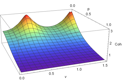
Figure 1: Quantum coherence $C(\rho_{ABC})$ of the GHZ state as functions of the mass parameter $\nu$ and the curvature parameter $p$.

In Fig.1, we plot quantum coherence $C(\rho_{ABC})$ as functions of the mass parameter $\nu$ and the curvature parameter $p$. From Fig.1, we can see that quantum coherence of the GHZ state decreases monotonically with the increase of the curvature parameter $p$. In other words, quantum coherence of the GHZ state increases with the increase of the curvature. This means that the curvature effect can improve quantum coherence in the multiverse. However, quantum coherence of the GHZ state decreases with the increase of the acceleration in Rindler spacetime, which means that the Unruh effect is harmful to quantum coherence L38 . This is a unique phenomenon of quantum coherence in de Sitter spaces. Conversely, quantum entanglement and discord decrease with the increase of the curvature in de Sitter spaces L25 ; L26 ; L27 ; L28 . This is also a unique phenomenon of quantum resources in de Sitter spaces. In addition, quantum coherence of the GHZ state is more sensitive to the curvature effect for $\nu\rightarrow 1/2$ (conformally coupled massless) and $\nu\rightarrow 3/2$ ( minimally coupled massless limit).

Tracing over the modes $A$, $B$ or $C$ from $\rho_{ABC}$, respectively, we obtain

$$\rho_{BC}= \frac{1}{2}\big{\{}(1-|\gamma_{p}|^{2})^{2}\sum_{n=0}^{\infty}\gamma_{p}^{2n}|n\rangle_{B}\langle n|\otimes(1-|\gamma_{p}|^{2})^{2}\sum_{m=0}^{\infty}\gamma_{p}^{2m}|m\rangle_{C}\langle m|$$ (32)

$$+ \sum_{n=0}^{\infty}\big{[}\frac{(1-|\gamma_{p}|^{2})^{2}}{2}\gamma_{p}^{2n}(n+1)(|n\rangle_{B}\langle n|+|n+1\rangle_{B}\langle n+1|)$$

$$+ \frac{(1-|\gamma_{p}|^{2})^{2}}{2}\gamma_{p}^{2n}\sqrt{n+1}\sqrt{n+2}(\gamma_{p}|n+2\rangle_{B}\langle n|+\gamma_{p}^{*}|n\rangle_{B}\langle n+2|)\big{]}$$

$$\otimes \sum_{m=0}^{\infty}\big{[}\frac{(1-|\gamma_{p}|^{2})^{2}}{2}\gamma_{p}^{2m}(m+1)(|m\rangle_{C}\langle m|+|m+1\rangle_{C}\langle m+1|)$$

$$+ \frac{(1-|\gamma_{p}|^{2})^{2}}{2}\gamma_{p}^{2m}\sqrt{m+1}\sqrt{m+2}(\gamma_{p}|m+2\rangle_{C}\langle m|+\gamma_{p}^{*}|m\rangle_{C}\langle m+2|)\big{]}\big{\}},$$

$$\rho_{AC}= \frac{1}{2}\big{\{}|0\rangle_{A}\langle 0|\otimes(1-|\gamma_{p}|^{2})^{2}\sum_{m=0}^{\infty}\gamma_{p}^{2m}|m\rangle_{C}\langle m|$$ (33)

$$+ |1\rangle_{A}\langle 1|\otimes\sum_{m=0}^{\infty}\big{[}(\frac{(1-|\gamma_{p}|^{2})^{2}}{2}\gamma_{p}^{2m}(m+1)|m\rangle_{C}\langle m|+|m+1\rangle_{C}\langle m+1|)$$

$$+ \frac{(1-|\gamma_{p}|^{2})^{2}}{2}\gamma_{p}^{2m}\sqrt{m+1}\sqrt{m+2}(\gamma_{p}|m+2\rangle_{C}\langle m|+\gamma_{p}^{*}|m\rangle_{C}\langle m+2|)\big{]}\big{\}},$$

$$\rho_{AB}= \frac{1}{2}\big{\{}|0\rangle_{A}\langle 0|\otimes(1-|\gamma_{p}|^{2})^{2}\sum_{m=0}^{\infty}\gamma_{p}^{2m}|m\rangle_{B}\langle m|$$ (34)

$$+ |1\rangle_{A}\langle 1|\otimes\sum_{m=0}^{\infty}\big{[}(\frac{(1-|\gamma_{p}|^{2})^{2}}{2}\gamma_{p}^{2m}(m+1)|m\rangle_{B}\langle m|+|m+1\rangle_{B}\langle m+1|)$$

$$+ \frac{(1-|\gamma_{p}|^{2})^{2}}{2}\gamma_{p}^{2m}\sqrt{m+1}\sqrt{m+2}(\gamma_{p}|m+2\rangle_{B}\langle m|+\gamma_{p}^{*}|m\rangle_{B}\langle m+2|)\big{]}\big{\}}.$$

Similarly, we get the density matrixs of the subsystem $A$, $B$ and $C$

$$\rho_{A}=\frac{1}{2}(|0\rangle_{A}\langle 0|+|1\rangle_{A}\langle 1|),$$ (35)

$$\rho_{B}= \frac{1}{2}\big{\{}|0\rangle_{B}\langle 0|+\sum_{m=0}^{\infty}\big{[}(\frac{(1-|\gamma_{p}|^{2})^{2}}{2}\gamma_{p}^{2m}(m+1)|m\rangle_{B}\langle m|+|m+1\rangle_{B}\langle m+1|)$$ (36)

$$+ \frac{(1-|\gamma_{p}|^{2})^{2}}{2}\gamma_{p}^{2m}\sqrt{m+1}\sqrt{m+2}(\gamma_{p}|m+2\rangle_{B}\langle m|+\gamma_{p}^{*}|m\rangle_{B}\langle m+2|)\big{]}\big{\}},$$

$$\rho_{C}= \frac{1}{2}\big{\{}|0\rangle_{C}\langle 0|+\sum_{m=0}^{\infty}\big{[}(\frac{(1-|\gamma_{p}|^{2})^{2}}{2}\gamma_{p}^{2m}(m+1)|m\rangle_{C}\langle m|+|m+1\rangle_{C}\langle m+1|)$$ (37)

$$+ \frac{(1-|\gamma_{p}|^{2})^{2}}{2}\gamma_{p}^{2m}\sqrt{m+1}\sqrt{m+2}(\gamma_{p}|m+2\rangle_{C}\langle m|+\gamma_{p}^{*}|m\rangle_{C}\langle m+2|)\big{]}\big{\}}.$$

Using Eq.(28), we obtain bipartite coherence as

$$C(\rho_{AB})=C(\rho_{AC})=\frac{(1-|\gamma_{p}|^{2})^{2}}{2}\sum_{n=0}^{\infty}\sqrt{n+2}\sqrt{n+1}|\gamma_{p}|^{2n+1},$$ (38)

$$C(\rho_{BC})= \frac{1}{2}\big{\{}[(1-|\gamma_{p}|^{2})^{2}\sum_{n=0}^{\infty}\sqrt{n+2}\sqrt{n+1}|\gamma_{p}|^{2n+1}]^{2}$$ (39)

$$+ 2(1-|\gamma_{p}|^{2})^{2}\sum_{n=0}^{\infty}\sqrt{n+2}\sqrt{n+1}|\gamma_{p}|^{2n+1}\big{\}}.$$

From Eqs.(35)-(37), we can find $C(\rho_{A})$ = 0 and $C(\rho_{AB})=C(\rho_{AC})=C(\rho_{B})=C(\rho_{C})$. This means that quantum coherence $C(\rho_{A})$ in the global chart of de Sitter space is always zero, while quantum coherence $C(\rho_{B})$ and $C(\rho_{C})$ in the $L$ region of de Sitter space can be generated by the curvature effect. However, the single particle coherence cannot be generated by the Unruh effect in Rindler spacetime L38 .

By calculation, we obtain an inequality $C(\rho_{BC})>C(\rho_{B})+C(\rho_{C})$, meaning that the curvature effect can generate nonlocal coherence between the modes $B$ and $C$ in de Sitter spaces. One can define the correlated coherence of a multipartite quantum system described by the density operator $\rho_{A_{1}\cdot\cdot\cdot A_{n}}$ L30 ; L31 ; L32 , which can be expressed as

$$C^{c}(\rho_{A_{1}\cdot\cdot\cdot A_{n}}):=C(\rho_{A_{1}\cdot\cdot\cdot A_{n}})-\sum_{i}^{n}C(\rho_{A_{i}}).$$ (40)

We obtain the correlated coherence as

$$C^{c}(\rho_{BC})=\frac{1}{2}[(1-|\gamma_{p}|^{2})^{2}\sum_{n=0}^{\infty}\sqrt{n+2}\sqrt{n+1}|\gamma_{p}|^{2n+1}]^{2},$$ (41)

$$C^{c}(\rho_{ABC})= \frac{1}{2}\big{\{}(1-|\gamma_{p}|^{2})^{3}\big{[}\sum_{n=0}^{\infty}\gamma_{p}^{2n}\sqrt{n+1}(1+|\gamma_{p}|)\big{]}^{2}$$ (42)

$$+(1-|\gamma_{p}|^{2})^{4}\big{[}\sum_{n=0}^{\infty}\gamma_{p}^{2n+1}\sqrt{n+1}\sqrt{n+2}\big{]}^{2}\big{\}}.$$

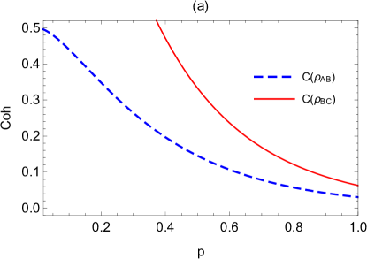
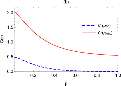
Figure 2: Bipartite coherence $C(\rho_{AB})$, $C(\rho_{BC})$, correlated coherence $C^{c}(\rho_{BC})$ and $C^{c}(\rho_{ABC})$ of the GHZ state as a function of the curvature parameter $p$ for a fixed $\nu=3/2$.

In Fig.2, we plot the bipartite coherence $C(\rho_{AB})$, $C(\rho_{BC})$, correlated coherence $C^{c}(\rho_{BC})$ and $C^{c}(\rho_{ABC})$ of the GHZ state as a function of the curvature parameter $p$ for a fixed $\nu=3/2$. We find that the bipartite (correlated) coherence decreases with the increase of the curvature parameter $p$, meaning that the curvature effect can generate the bipartite (correlated) coherence. However, the Unruh effect cannot generate bipartite (correlated) coherence in Rindler spacetime L38 . This the difference is due to the perfect symmetry of de Sitter spaces.

III.2 Tripartite W state

In this section, we assume that initially Alice, Bob, and Charlie share the W state

$$|W\rangle = \frac{1}{\sqrt{3}}[|0\rangle_{A,\rm BD_{1}}|0\rangle_{B,\rm BD_{2}}|1\rangle_{C,\rm BD_{3}}+|0\rangle_{A,\rm BD_{1}}|1\rangle_{B,\rm BD_{2}}|0\rangle_{C,\rm BD_{3}}$$

$$+ |1\rangle_{A,\rm BD_{1}}|0\rangle_{B,\rm BD_{2}}|0\rangle_{C,\rm BD_{3}}].$$

Following the treatment for the GHZ state, the W state becomes

$$\begin{aligned} |W\rangle_{AB\bar{B}C\bar{C}}=&\frac{(1-|\gamma_{p}|^{2})^{\frac{3}{2}}}{\sqrt{6}}\sum_{n,m=0}^{\infty}\gamma_{p}^{n}\gamma_{p}^{m}\big{[}\sqrt{m+1}|0\rangle_{A}|n\rangle_{B}|n\rangle_{\bar{B}}(|m\rangle_{C}|m+1\rangle_{\bar{C}}\\ +&|(m+1)\rangle_{C}|m\rangle_{\bar{C}})+\sqrt{n+1}|0\rangle_{A}(|n\rangle_{B}|n+1\rangle_{\bar{B}}+|n+1\rangle_{B}+|n\rangle_{\bar{B}})\\ \otimes&|m\rangle_{C}|m\rangle_{\bar{C}}+\sqrt{2}(1-|\gamma_{p}|^{2})^{-\frac{1}{2}}|1\rangle_{A}|n\rangle_{B}|n\rangle_{\bar{B}}|m\rangle_{C}|m\rangle_{\bar{C}}\big{]}.\end{aligned}$$ (44)

The reduced density matrix after tracing over the modes $\bar{B}$ and $\bar{C}$ can be expressed as

$$\rho_{ABC}=\frac{1}{3}\sum_{n,m=0}^{\infty}\gamma_{p}^{2n}\gamma_{p}^{2m}\rho_{n,m}$$ (45)

$$\rho_{n,m}= |0\rangle_{A}\langle 0|\otimes(1-|\gamma_{p}|^{2})|n\rangle_{B}\langle n|\otimes\frac{(1-|\gamma_{p}|^{2})^{2}}{2}[(m+1)(|m\rangle_{C}\langle m|+|m+1\rangle_{C}\langle m+1|)$$ (46)

$$+ \sqrt{m+2}\sqrt{m+1}(\gamma_{p}^{*}|m\rangle_{C}\langle m+2|+\gamma_{p}|m+2\rangle_{C}\langle m|)]$$

$$+ |0\rangle_{A}\langle 0|\otimes\frac{(1-|\gamma_{p}|^{2})^{2}}{2}[(n+1)(|n\rangle_{B}\langle n|+|n+1\rangle_{B}\langle n+1|)$$

$$+ \sqrt{n+1}\sqrt{n+2}(\gamma_{p}^{*}|n\rangle_{B}\langle n+2|+\gamma_{p}|n+2\rangle_{B}\langle n|)](1-|\gamma_{p}|^{2})\otimes|m\rangle_{C}\langle m|$$

$$+ [|0\rangle_{A}\langle 0|\otimes\frac{(1-|\gamma_{p}|^{2})^{\frac{3}{2}}}{\sqrt{2}}\sqrt{n+1}[|n\rangle_{B}\langle n+1|+\gamma_{p}|n+1\rangle_{B}\langle n|]$$

$$\otimes \frac{(1-|\gamma_{p}|^{2})^{\frac{3}{2}}}{\sqrt{2}}\sqrt{m+1}[\gamma_{p}^{*}|m\rangle_{C}\langle m+1|+|m+1\rangle_{C}\langle m|]+h.c.]+[|0\rangle_{A}\langle 1||n\rangle_{B}\langle n|$$

$$\otimes \frac{(1-|\gamma_{p}|^{2})^{\frac{3}{2}}}{\sqrt{2}}\sqrt{m+1}[\gamma_{p}^{*}|m\rangle_{C}\langle m+1|+|m+1\rangle_{C}\langle m|]+h.c.]$$

$$+ [|1\rangle_{A}\langle 0|\otimes\frac{(1-|\gamma_{p}|^{2})^{\frac{3}{2}}}{\sqrt{2}}\sqrt{n+1}[|n\rangle_{B}\langle n+1|+\gamma_{p}|n+1\rangle_{B}\langle n|]\otimes|m\rangle_{C}\langle m|+h.c.]$$

$$+ (1-|\gamma_{p}|^{2})^{2}{[|1\rangle_{A}\langle 1||n\rangle_{B}\langle n||m\rangle_{C}\langle m|]}.$$

Employing Eq.(28), the coherence of the W state becomes

$$C(\rho_{ABC})= \frac{1}{3}\big{\{}2(1-|\gamma_{p}|^{2})^{2}\sum_{n=0}^{\infty}|\gamma_{p}|^{2n+1}\sqrt{n+2}\sqrt{n+1}$$ (47)

$$+ 2\sqrt{2}(1-|\gamma_{p}|^{2})^{\frac{3}{2}}\sum_{m=0}^{\infty}|\gamma_{p}|^{2m}\sqrt{m+1}(|\gamma_{p}|+1)$$

$$+ (1-|\gamma_{p}|^{2})^{3}[\sum_{m=0}^{\infty}|\gamma_{p}|^{2m}\sqrt{m+1}(|\gamma_{p}|+1)]^{2}\big{\}}.$$

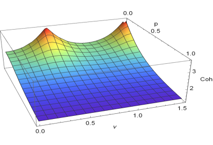
Figure 3: Quantum coherence $C(\rho_{ABC})$ of the W state as functions of the mass parameter $\nu$ and the curvature parameter $p$.

In Fig.3, quantum coherence $C(\rho_{ABC})$ of the W state is plotted as functions of the mass parameter $\nu$ and the curvature parameter $p$. From Fig.3, we can see that quantum coherence of the W state decreases monotonically with the increase of curvature parameter $p$, which means that quantum coherence increases monotonically with the increase of the curvature. Conversely, quantum coherence of the W state decreases monotonously with the increase of the acceleration in Rindler spacetime L38 . This proves again that the curvature effect is beneficial to quantum coherence in de Sitter spaces, and the Unruh effect damages quantum coherence in Rindler spacetime. From Fig.3, we also see that quantum coherence of the W state is most severely affected by the curvature effect of de Sitter space for $\nu\rightarrow 1/2$ (conformally coupled massless) and $\nu\rightarrow 3/2$ ( minimally coupled massless limit). In addition, quantum coherence of the W state is larger than that of the GHZ state, which means that quantum coherence of the W state is more suitable for processing quantum information tasks in the multiverse.

We get the density matrix $\rho_{BC}$, $\rho_{AC}$ and $\rho_{AB}$ after tracing over the modes $A$, $B$, or $C$ from the state $\rho_{ABC}$, respectively,

$$\rho_{BC}= \frac{1}{3}[[(1-|\gamma_{p}|^{2})\sum_{n=0}^{\infty}\gamma_{p}^{2n}|n\rangle_{B}\langle n|\otimes\frac{(1-|\gamma_{p}|^{2})^{2}}{2}\sum_{m=0}^{\infty}\gamma_{p}^{2m}[(m+1)(|m\rangle_{C}\langle m|$$ (48)

$$+ |m+1\rangle_{C}\langle m+1|)+\sqrt{m+1}\sqrt{m+2}(\gamma_{p}|m+2\rangle_{C}\langle m|+\gamma_{p}^{*}|m\rangle_{C}\langle m+2|)]+h.c.]$$

$$+ [\frac{(1-|\gamma_{p}|^{2})^{\frac{3}{2}}}{\sqrt{2}}\sum_{n=0}^{\infty}\gamma_{p}^{2n}\sqrt{n+1}(|n\rangle_{B}\langle n+1|+\gamma_{p}|n+1\rangle_{B}\langle n|)$$

$$\otimes \frac{(1-|\gamma_{p}|^{2})^{\frac{3}{2}}}{\sqrt{2}}\sum_{m=0}^{\infty}\gamma_{p}^{2m}\sqrt{m+1}(|m+1\rangle_{C}\langle m|+\gamma_{p}^{*}|m\rangle_{C}\langle m+1|)+h.c.]$$

$$+ (1-|\gamma_{p}|^{2})\sum_{n=0}^{\infty}\gamma_{p}^{2n}|n\rangle_{B}\langle n|\otimes(1-|\gamma_{p}|^{2})\sum_{m=0}^{\infty}\gamma_{p}^{2m}|m\rangle_{C}\langle m|],$$

$$\rho_{AC}= \frac{1}{3}[|0\rangle_{A}\langle 0|\otimes\frac{(1-|\gamma_{p}|^{2})^{2}}{2}\sum_{m=0}^{\infty}\gamma_{p}^{2m}[(m+1)(|m\rangle_{B}\langle m|+|m+1\rangle_{B}\langle m+1|)$$ (49)

$$+ \sqrt{m+1}\sqrt{m+2}(\gamma_{p}|m+2\rangle_{B}\langle m|+\gamma_{p}^{*}|m\rangle_{B}\langle m+2|)]$$

$$+ |0\rangle_{A}\langle 1|\otimes\frac{(1-|\gamma_{p}|^{2})^{\frac{3}{2}}}{\sqrt{2}}\sum_{m=0}^{\infty}\gamma_{p}^{2m}\sqrt{m+1}(|m+1\rangle_{B}\langle m|+\gamma_{p}^{*}|m\rangle_{B}\langle m+1|)$$

$$+ |1\rangle_{A}\langle 0|\otimes\frac{(1-|\gamma_{p}|^{2})^{\frac{3}{2}}}{\sqrt{2}}\sum_{m=0}^{\infty}\gamma_{p}^{2m}\sqrt{m+1}(|m+1\rangle_{B}\langle m|+\gamma_{p}^{*}|m\rangle_{B}\langle m+1|)$$

$$+ |0\rangle_{A}\langle 0|\otimes(1-|\gamma_{p}|^{2})\sum_{m=0}^{\infty}\gamma_{p}^{2m}|m\rangle_{B}\langle m|+|1\rangle_{A}\langle 1|\otimes(1-|\gamma_{p}|^{2})\sum_{m=0}^{\infty}\gamma_{p}^{2m}|m\rangle_{B}\langle m|],$$

$$\rho_{AB}= \frac{1}{3}[|0\rangle_{A}\langle 0|\otimes\frac{(1-|\gamma_{p}|^{2})^{2}}{2}\sum_{m=0}^{\infty}\gamma_{p}^{2m}[(m+1)(|m\rangle_{C}\langle m|+|m+1\rangle_{C}\langle m+1|)$$ (50)

$$+ \sqrt{m+1}\sqrt{m+2}(\gamma_{p}|m+2\rangle_{C}\langle m|+\gamma_{p}^{*}|m\rangle_{C}\langle m+2|)]$$

$$+ |0\rangle_{A}\langle 1|\otimes\frac{(1-|\gamma_{p}|^{2})^{\frac{3}{2}}}{\sqrt{2}}\sum_{m=0}^{\infty}\gamma_{p}^{2m}\sqrt{m+1}(|m+1\rangle_{C}\langle m|+\gamma_{p}^{*}|m\rangle_{C}\langle m+1|)$$

$$+ |1\rangle_{A}\langle 0|\otimes\frac{(1-|\gamma_{p}|^{2})^{\frac{3}{2}}}{\sqrt{2}}\sum_{m=0}^{\infty}\gamma_{p}^{2m}\sqrt{m+1}(|m+1\rangle_{C}\langle m|+\gamma_{p}^{*}|m\rangle_{C}\langle m+1|)$$

$$+ |0\rangle_{A}\langle 0|\otimes(1-|\gamma_{p}|^{2})\sum_{m=0}^{\infty}\gamma_{p}^{2m}|m\rangle_{C}\langle m|+|1\rangle_{A}\langle 1|\otimes(1-|\gamma_{p}|^{2})\sum_{m=0}^{\infty}\gamma_{p}^{2m}|m\rangle_{C}\langle m|].$$

Using Eq.(28), we obtain the bipartite coherence as

$$C(\rho_{BC})= \frac{1}{3}\big{\{}2(1-|\gamma_{p}|^{2})^{2}\sum_{n=0}^{\infty}\sqrt{n+1}\sqrt{n+2}|\gamma_{p}|^{2n+1}$$ (51)

$$+ (1-|\gamma_{p}|^{2})^{3}\big{[}\sum_{n=0}^{\infty}|\gamma_{p}|^{2n}\sqrt{n+1}(|\gamma_{p}|+1)\big{]}^{2}\big{\}},$$

$$C(\rho_{AC})=C(\rho_{AB})= \frac{1}{3}[(1-|\gamma_{p}|^{2})^{2}\sum_{n=0}^{\infty}\sqrt{n+1}\sqrt{n+2}|\gamma_{p}|^{2n+1}$$ (52)

$$+ \sqrt{2}(1-|\gamma_{p}|^{2})^{\frac{3}{2}}\sum_{n=0}^{\infty}|\gamma_{p}|^{2n}\sqrt{n+1}(1+|\gamma_{p}|)].$$

Similarly, we get the density matrices $\rho_{A},\rho_{B}$, and $\rho_{C}$ of single particle system as

$$\rho_{A}=\frac{1}{3}(2|0\rangle_{A}\langle 0|+|1\rangle_{A}\langle 1|),$$ (53)

$$\rho_{B}= \frac{1}{3}[2(1-|\gamma_{p}|^{2})\sum_{m=0}^{\infty}\gamma_{p}^{2m}|m\rangle_{B}\langle m|+\frac{(1-|\gamma_{p}|^{2})^{2}}{2}\sum_{m=0}^{\infty}\gamma_{p}^{2m}[(m+1)(|m\rangle_{B}\langle m|$$ (54)

$$+ |m+1\rangle_{B}\langle m+1|)+\sqrt{m+1}\sqrt{m+2}(\gamma_{p}|m+2\rangle_{B}\langle m|+\gamma_{p}^{*}|m\rangle_{B}\langle m+2|)]],$$

$$\rho_{C}= \frac{1}{3}[2(1-|\gamma_{p}|^{2})\sum_{m=0}^{\infty}\gamma_{p}^{2m}|m\rangle_{C}\langle m|+\frac{(1-|\gamma_{p}|^{2})^{2}}{2}\sum_{m=0}^{\infty}\gamma_{p}^{2m}[(m+1)(|m\rangle_{C}\langle m|$$ (55)

$$+ |m+1\rangle_{C}\langle m+1|)+\sqrt{m+1}\sqrt{m+2}(\gamma_{p}|m+2\rangle_{C}\langle m|+\gamma_{p}^{*}|m\rangle_{C}\langle m+2|)]].$$

The corresponding single particle coherence reads

$$C(\rho_{A})=0,$$ (56)

$$C(\rho_{B})=C(\rho_{C})= \frac{(1-|\gamma_{p}|^{2})^{2}}{3}\sum_{n=0}^{\infty}\sqrt{n+1}\sqrt{n+2}|\gamma_{p}|^{2n+1}.$$ (57)

According to Eq.(37), we can obtain the correlated coherence as

$$C^{c}(\rho_{ABC})= \frac{1}{3}\big{\{}2\sqrt{2}(1-|\gamma_{p}|^{2})^{\frac{3}{2}}\sum_{m=0}^{\infty}|\gamma_{p}|^{2m}\sqrt{m+1}(|\gamma_{p}|+1)$$ (58)

$$+ (1-|\gamma_{p}|^{2})^{3}[\sum_{m=0}^{\infty}|\gamma_{p}|^{2m}\sqrt{m+1}(|\gamma_{p}|+1)]^{2}\big{\}},$$

$$C^{c}(\rho_{AB})=C^{c}(\rho_{AC})= \frac{\sqrt{2}(1-|\gamma_{p}|^{2})^{\frac{3}{2}}}{3}\sum_{n=0}^{\infty}|\gamma_{p}|^{2n}\sqrt{n+1}(|\gamma_{p}|+1),$$ (59)

$$C^{c}(\rho_{BC})= \frac{(1-|\gamma_{p}|^{2})^{3}}{3}\big{[}\sum_{n=0}^{\infty}|\gamma_{p}|^{2n}\sqrt{n+1}(|\gamma_{p}|+1)\big{]}^{2}.$$ (60)

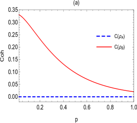
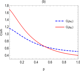
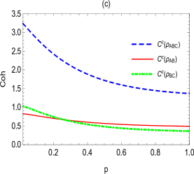
Figure 4: Single particle coherence $C(\rho_{A})$ and $C(\rho_{B})$, bipartite coherence $C(\rho_{BC})$ and $C(\rho_{AB})$, and correlated coherence $C^{c}(\rho_{AB})$, $C^{c}(\rho_{BC})$ and $C^{c}(\rho_{ABC})$ of the W state as a function of the curvature parameter $p$ for a fixed $\nu=3/2$.

In Fig.4, we plot the single particle coherence $C(\rho_{A})$ and $C(\rho_{B})$, bipartite coherence $C(\rho_{BC})$ and $C(\rho_{AB})$, and correlated coherence $C^{c}(\rho_{AB})$, $C^{c}(\rho_{BC})$ and $C^{c}(\rho_{ABC})$ of the W state as a function of the curvature parameter $p$ for a fixed $\nu=3/2$. From Fig.4, we can see that the single particle coherence $C(\rho_{A})$ in a global chart is zero, while the curvature effect can produce the single coherence $C(\rho_{B})$ (or $C(\rho_{C})$) in the $L$ region of de Sitter space. Conversely, the Unruh effect cannot generate the single particle coherence of the W state in Rindler spacetime L38 ; L39 . We can also see that the bipartite coherence $C(\rho_{BC})$ is not always bigger than the bipartite coherence $C(\rho_{AB})$ (or $C(\rho_{AC})$ in the multiverse. We find that the bipartite (or tripartite ) coherence is bigger that its correlated coherence in de Sitter spaces, while the bipartite (or tripartite ) coherence equals its correlated coherence in Rindler spacetime.

The relationship of quantum coherence for the W state is still unclear in the multiverse. Through direct calculation, we obtain a distribution relationship between the correlated coherence of the tripartite W state as

$$C^{c}(\rho_{ABC})= C^{c}(\rho_{AB})+C^{c}(\rho_{BC})+C^{c}(\rho_{AC}).$$ (61)

From Eq.(61), we can see that the correlated coherence of the W state exists essentially in the form of bipartite correlated coherence, showing that the correlated coherence of the tripartite system is equal to the sum of all the bipartite correlated coherence in the multiverse. However, quantum coherence of the W state is equal to the sum of all the bipartite system of quantum coherence in Rindler spacetime L38 ; L39 . This is a difference between de Sitter space and Rindler spacetime.

The preceding analysis reveals that multipartite coherence in de Sitter space exhibits behaviors that are fundamentally distinct from that observed in Rindler spacetime L38 ; L39 . In the subsequent discussion, our aim is to elucidate the origins of these different behaviors from the perspective of Bogoliubov transformation. The Minkowski vacuum and excitation states observed by an inertial observer are interconnected with the states of the $I$ and $II$ regions in Rindler spacetime in the following manner

$$|0\rangle_{\rm M}=\frac{1}{\cosh(\gamma)}\sum_{n=0}^{\infty}\tanh^{n}(\gamma)|n\rangle_{\rm I}|n\rangle_{\rm{II}},$$ (62)

$$|1\rangle_{\rm M}=\frac{1}{\cosh^{2}(\gamma)}\sum_{n=0}^{\infty}\tanh^{n}(\gamma)\sqrt{n+1}|n+1\rangle_{\rm I}|n\rangle_{\rm{II}},$$ (63)

where $\gamma$ is the acceleration parameter. It is observed that this transformation given by Eq.(62) displays symmetry concerning the $I$ and $II$ regions, while the transformation described by Eq.(63) exhibits asymmetry in relation to the $I$ and $II$ regions. However, the transformation provided by Eqs.(17) and (18) demonstrates symmetry concerning the $R$ and $L$ regions. It is this symmetry and asymmetry of transformations that results in different behaviors of quantum coherence. Specifically, Eqs.(17) and (18) govern the evolution of density matrices from the Bunch-Davies basis to the basis of the open chart $L$ region

$$\rm{Tr_{R}(|0\rangle_{BD}\langle 0|)}=(1-|\gamma_{p}|^{2})\sum_{n=0}^{\infty}|\gamma_{p}|^{2n}|n\rangle_{\rm L}\langle n|,$$ (64)

$$\rm{Tr_{R}(|0\rangle_{BD}\langle 1|)} = (1-|\gamma_{p}|^{2})^{\frac{3}{2}}\sum_{n=0}^{\infty}|\gamma_{p}|^{2n}\sqrt{\frac{n+1}{2}}$$ (65)

$$(\gamma_{p}|n+1\rangle_{\rm L}\langle n|+|n\rangle_{\rm L}\langle n+1|),$$

$$\rm{Tr_{R}(|1\rangle_{BD}\langle 1|)} = \frac{(1-|\gamma_{p}|^{2})^{2}}{2}\sum_{n=0}^{\infty}|\gamma_{p}|^{2n}[(n+1)(|n\rangle_{\rm L}\langle n|+|n+1\rangle_{\rm L}\langle n+1|)$$ (66)

$$+ \sqrt{(n+1)(n+2)}(\gamma_{p}|n+2\rangle_{\rm L}\langle n|+\gamma_{p}^{*}|n\rangle_{\rm L}\langle n+2|)].$$

Likewise, Eqs.(62) and (63) drive the evolution of density matrices from the Minkowski basis to the basis of the $I$ region of Rindler spacetime, as represented by

$$\rm{Tr_{II}(|0\rangle_{M}\langle 0|)}=\frac{1}{\cosh^{2}\gamma}\sum_{n=0}^{\infty}\tanh^{2n}\gamma|n\rangle_{\rm I}\langle n|,$$ (67)

$$\rm{Tr_{II}(|0\rangle_{M}\langle 1|)}=\frac{1}{\cosh^{3}\gamma}\sum_{n=0}^{\infty}\tanh^{2n}\gamma\sqrt{n+1}|n\rangle_{\rm I}\langle n+1|,$$ (68)

$$\rm{Tr_{II}(|1\rangle_{M}\langle 1|)}=\frac{1}{\cosh^{4}\gamma}\sum_{n=0}^{\infty}\tanh^{2n}\gamma(n+1)|n+1\rangle_{\rm I}\langle n+1|.$$ (69)

Upon comparing Eqs.(64)-(66) with Eqs.(67)-(69), we identify the distinctions in the evolution of density matrices: (i) the curvature effect of de Sitter space can induce the generation of non-diagonal elements in the basis of the open chart $L$ region from the originally diagonal elements of the density matrix in the Bunch-Davies basis $(|1\rangle_{\rm{BD}}\langle 1|)$ [see Eq.(66)], showing that the diagonal element $(|1\rangle_{\rm{BD}}\langle 1|)$ has a positive contribution to quantum coherence; (ii) the acceleration effect fails to generate non-diagonal elements in the $I$ region of Rindler spacetime from the diagonal elements of the density matrix in the Minkowski basis [see Eqs.(67) and (69)], meaning that the diagonal element has no contribution to quantum coherence; (iii) clearly, the non-diagonal element $(|0\rangle_{\rm{BD}}\langle 1|)$ [see Eq.(65)] and its conjugation consistently contribute positively to quantum coherence through the curvature effect of de Sitter space; (iv) obviously, the non-diagonal element $(|0\rangle_{M}\langle 1|)$ [see Eq.(68)] and its conjugation always have a negative contribution to quantum coherence via the Unruh effect of Rindler spacetime.

IV N-partite coherence in multiverse

In this section, we will discuss the extension of the tripartite systems to the N-partite systems ($N$ $\geq 3$). The N-partite GHZ state and N-partite W state can be written as

$$|GHZ\rangle_{123\cdot\cdot\cdot N} = \frac{1}{\sqrt{2}}(|0\rangle_{\rm BD,1}|0\rangle_{\rm BD,2}...|0\rangle_{\rm BD,(N-1)}|0\rangle_{\rm BD,N}$$ (70)

$$+ |1\rangle_{\rm BD,1}|1\rangle_{\rm BD,2}...|1\rangle_{\rm BD,(N-1)}|1\rangle_{\rm BD,N}),$$

$$|W\rangle_{123\cdot\cdot\cdot N}= \frac{1}{N}(|1\rangle_{\rm BD,1}|0\rangle_{\rm BD,2}..|0\rangle_{\rm BD,(N-1)}|0\rangle_{\rm BD,N}+|0_{\rm BD,1}|1\rangle_{\rm BD,2}...|0_{\rm BD,(N-1)}|0\rangle_{\rm BD,N}$$ (71)

$$+\cdot\cdot\cdot+|0_{\rm BD,1}|0\rangle_{\rm BD,2}...|0\rangle_{\rm BD,(N-1)}|1\rangle_{\rm BD,N}),$$

where the mode $i$ ($i=1,2,...,N$)) is observed by observer $O_{i}$ in de Sitter space $\rm BD_{i}$. Now we assume that $n$ ($2\leq n\leq N-1$) observers are in the different $L$ regions of the expanded de Sitter spaces and $N-n$ observers are in global charts of the other de Sitter spaces. By a series of calculations, we obtain N-partite coherence of the GHZ and W states as

$$C(GHZ)= \frac{1}{2}\bigg{\{}2\bigg{[}\frac{(1-|\gamma_{p}|^{2})^{\frac{3}{2}}}{\sqrt{2}}\sum_{m=0}^{\infty}|\gamma_{p}|^{2m}\sqrt{m+1}(|\gamma_{p}|+1)\bigg{]}^{n}$$ (72)

$$+ \bigg{[}1+(1-|\gamma_{p}|^{2})^{2}\sum_{m=0}^{\infty}|\gamma_{p}|^{2m+1}\sqrt{m+1}\sqrt{m+2}\bigg{]}^{n}-1\bigg{\}},$$

$$C(W)= \frac{1}{N}\bigg{\{}n(1-|\gamma_{p}|^{2})^{2}\sum_{m=0}^{\infty}\sqrt{m+1}\sqrt{m+2}|\gamma_{p}|^{2m+1}$$ (73)

$$+ 2n(N-n)\frac{(1-|\gamma_{p}|^{2})^{\frac{3}{2}}}{\sqrt{2}}\sum_{m=0}^{\infty}|\gamma_{p}|^{2m}\sqrt{m+1}(|\gamma_{p}|+1)$$

$$+ n(n-1)[\frac{(1-|\gamma_{p}|^{2})^{\frac{3}{2}}}{\sqrt{2}}\sum_{m=0}^{\infty}|\gamma_{p}|^{2m}\sqrt{m+1}(|\gamma_{p}|+1)]^{2}$$

$$+ (N-n)(N-n-1)\bigg{\}}.$$

After tedious but straightforward calculations, the correlated coherence of the GHZ and W states reads

$$C^{c}(GHZ)= \frac{1}{2}\bigg{\{}2\bigg{[}\frac{(1-|\gamma_{p}|^{2})^{\frac{3}{2}}}{\sqrt{2}}\sum_{m=0}^{\infty}|\gamma_{p}|^{2m}\sqrt{m+1}(|\gamma_{p}|+1)\bigg{]}^{n}$$ (74)

$$+ \bigg{[}1+(1-|\gamma_{p}|^{2})^{2}\sum_{m=0}^{\infty}|\gamma_{p}|^{2m+1}\sqrt{m+1}\sqrt{m+2}\bigg{]}^{n}-1$$

$$- n(1-|\gamma_{p}|^{2})^{2}\sum_{m=0}^{\infty}|\gamma_{p}|^{2m+1}\sqrt{m+1}\sqrt{m+2}\bigg{\}},$$

$$C^{c}(W)= \frac{1}{N}\bigg{[}2n(N-n)\frac{(1-|\gamma_{p}|^{2})^{\frac{3}{2}}}{\sqrt{2}}\sum_{m=0}^{\infty}|\gamma_{p}|^{2m}\sqrt{m+1}(|\gamma_{p}|+1)$$ (75)

$$+ n(n-1)[\frac{(1-|\gamma_{p}|^{2})^{\frac{3}{2}}}{\sqrt{2}}\sum_{m=0}^{\infty}|\gamma_{p}|^{2m}\sqrt{m+1}(|\gamma_{p}|+1)]^{2}$$

$$+ (N-n)(N-n-1)\bigg{]}.$$

From Eqs.(72)-(75), we can see that N-partite (correlated ) coherence of the GHZ state depends only on the $n$ observers who are in the different $L$ regions of the expanded de Sitter spaces, while N-partite (correlated ) coherence of the W state depends not only on the $n$ observers but also on the initial $N$ observers.

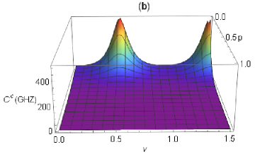
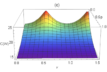
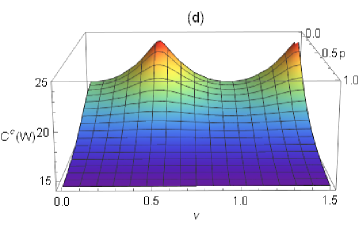
Figure 5: N-partite coherence and correlated coherence of the GHZ and W states as functions of the mass parameter $\nu$ and the curvature parameter $p$ for fixed $n$=10 and $N$=20.

In Fig.5, we plot N-partite coherence and correlated coherence of the GHZ and W states as functions of the curvature parameter $p$ and the mass parameter $\nu$, assuming $n$ = 10 and $N$ = 20. We find that the curvature effect enhances N-partite (correlated) coherence. Therefore, the curvature effect is beneficial to N-partite (correlated) coherence in the multiverse consisting of many de Sitter spaces, while the Unruh effect is harmful to N-partite coherence in Rindler spacetime L38 .

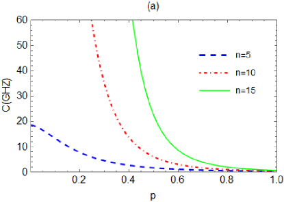
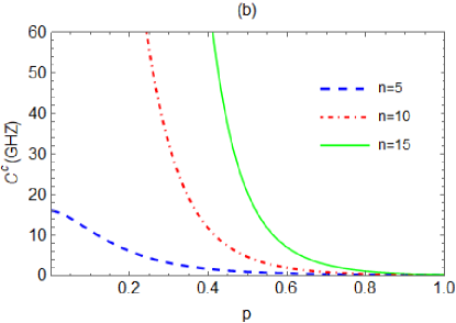
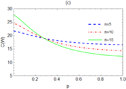
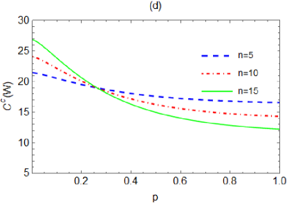
Figure 6: N-partite coherence and correlated coherence of the GHZ and W states as a function of the curvature parameter $p$ for fixed $\nu=3/2$, $N$ = 20 and different $n$.

In Fig.6, N-partite coherence and correlated coherence of the GHZ and W states are plotted as a function of the curvature parameter $p$ for different $n$. From Fig.6 (a)-(b), we can see that N-partite (correlated) coherence of the GHZ state increases monotonically with increasing $n$ for any curvature parameter $p$. From Fig.6 (c)-(d), we can also see that, with the increase of $n$, N-partite (correlated) coherence of the W state for smaller curvature parameter $p$ increases monotonically, while for larger curvature parameter $p$ decreases monotonically in the multiverse. However, N-partite (correlated) coherence of the GHZ and W states for any acceleration parameter decreases monotonically with the increase of the accelerated observers $n$ L38 .

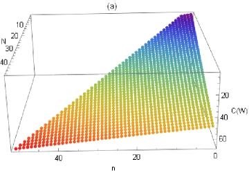
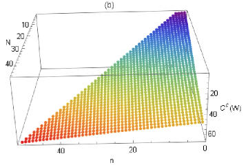
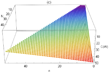
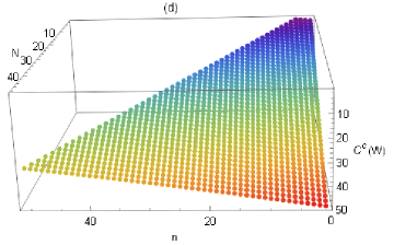
Figure 7: N-partite coherence and correlated coherence of the W state as functions of $n$ and $N$ for $p=0.1$ (a) and (b), $p=0.6$ (c) and (d). The parameter $\nu$ is fixed as $\nu=3/2$.

In Fig.7, we describe N-partite coherence and correlated coherence of the W state as functions of $n$ and $N$ for different $p$. From Fig.7, we can see that N-partite (correlated) coherence of the W state increases monotonically with the increase of $N$ for any $p$ and $n$, while N-partite (correlated) coherence of the GHZ state is independent of $N$. We can also see that N-partite (correlated) coherence of the W state increases or decreases monotonically with the growth of $n$ depending on the curvature parameter $p$.

Next, we study the distribution relationship of coherence for the N-partite systems in the multiverse. For N-partite W state, the distribution relationship of the correlated coherence can be written as

$$\frac{n(n-1)}{2}C^{c}(\rho_{O}\rho_{O})+n(N-n)C^{c}(\rho_{O}\rho_{X})+\frac{(N-n)(N-n-1)}{2}C^{c}(\rho_{X}\rho_{X})=C^{c}(W).$$ (76)

Here,

$$C^{c}(\rho_{O}\rho_{O})=\frac{2}{N}[\frac{(1-|\gamma_{p}|^{2})^{\frac{3}{2}}}{\sqrt{2}}\sum_{m=0}^{\infty}|\gamma_{p}|^{2m}\sqrt{m+1}(|\gamma_{p}|+1)]^{2}$$

denotes the bipartite correlated coherence of the modes corresponding to two observers in the $L$ regions of the expanded de Sitter spaces;

$$C^{c}(\rho_{O}\rho_{X})=\frac{2}{N}\frac{(1-|\gamma_{p}|^{2})^{\frac{3}{2}}}{\sqrt{2}}\sum_{m=0}^{\infty}|\gamma_{p}|^{2m}\sqrt{m+1}(|\gamma_{p}|+1)$$

denotes the bipartite correlated coherence of the modes corresponding to two observers who are, respectively, in the $L$ region of the expanded de Sitter space and the global chart of de Sitter space; $C^{c}(\rho_{X}\rho_{X})=\frac{2}{N}$ denotes the bipartite correlated coherence of the modes corresponding to two observers in the global chart of de Sitter spaces. From Eq.(76), we can see that the total correlated coherence of N-partite W state is equal to the sum of all bipartite correlated coherence in the multiverse.

V Conclutions

The curvature effect on quantum coherence of tripartite GHZ and W states in the multiverse has been investigated. It is shown that tripartite coherence increases with the increase of the curvature, meaning that the curvature effect is beneficial to quantum coherence in the multiverse. However, with the growth of the curvature, quantum entanglement gradually vanishes and quantum discord gradually decreases to a fixed value at the limit of infinite curvature in de Sitter space L25 ; L26 ; L27 ; L28 . Conversely, tripartite coherence decreases with increasing acceleration in Rindler spacetime, showing that the Unruh effect is harmful to quantum coherence L38 . Therefore, the results reflect the unique property of the de Sitter expansion, which is not similar to the case of the Unruh effect in Rindler spacetime. We find that quantum coherence of the GHZ and W states is sensitive to the curvature effect in the limit of conformal and massless scalar fields. Interestingly, the curvature effect can generate bipartite quantum coherence and single-partite quantum coherence, but the Unruh effect cannot. We obtain a distribution relationship of correlated coherence for the W state in the multiverse. In other words, tripartite correlated coherence of the W state is equal to the sum of all bipartite correlated coherence.

We have extended the investigation from the tripartite systems to N-partite systems in the multiverse. Unlike tripartite coherence, N-partite coherence of the W state depends not only on the curvature and mass parameters, but also on the $n$ particles in the $L$ regions of the de Sitter spaces and the initial $N$ particles. However, N-partite coherence of the GHZ state is independent of the $N$. We find that with the increase of the $n$, N-partite coherence of the GHZ state increases monotonically for any curvature, while N-partite coherence of the W state increases or decreases monotonically, depending on the curvature. We extend the tripartite distribution relationship to the N-partite distribution relationship. This indicates that the total correlated coherence of N-partite W state is essentially bipartite types. Based on the above arguments, we expect that multipartite coherence will be able to provide some evidence for the existence of the multiverse.

- (1) A. J. Leggett, Macroscopic Quantum Systems and the Quantum Theory of Measurement, Prog. Theor. Phys. Suppl. 69, 80 (1980).
- (2) B. Schumacher and M. D. Westmoreland, Quantum Privacy and Quantum Coherence, Phys. Rev. Lett. 80, 5695 (1998).
- (3) S. E. Barnes, R. Ballou, B. Barbara and J. Strelen, Quantum Coherence in Small Antiferromagnets, Phys. Rev. Lett. 79, 289 (1997).
- (4) A. Streltsov, G. Adesso and M. B. Plenio, Colloquium: Quantum coherence as a resource, Rev. Mod. Phys. 89, 041003 (2017).
- (5) U. K. Sharma, I. Chakrabarty and M. K. Shukla, Broadcasting quantum coherence via cloning, Phys. Rev. A 96, 052319 (2017).
- (6) Y. Peng, Y. Jiang and H. Fan, Maximally coherent states and coherence-preserving operations, Phys. Rev. A 93, 032326 (2016).
- (7) F. Brandão, M. Horodecki, N. Ng, J. Oppenheim and S. Wehner, The second laws of quantum thermodynamics, Proc. Natl Acad. Sci. USA 112 3275 (2015).
- (8) M. Horodecki and J. Oppenheim, Fundamental limitations for quantum and nanoscale thermodynamics, Nat. Commun. 4, 2059 (2013).
- (9) P. Ćwikliński, M. Studziński, M. Horodecki and J. Oppenheim, Limitations on the Evolution of Quantum Coherences: Towards Fully Quantum Second Laws of Thermodynamics, Phys. Rev. Lett. 115, 210403 (2015).
- (10) S. F. Huelga and M. B. Plenio, A vibrant environment, Nat. Phys. 10, 621 (2014).
- (11) S. F. Huelga and M. B. Plenio, Vibrations, Quanta and Biology, Contemp. Phys. 54, 181 (2013).
- (12) M. Gärttner, P. Hauke and A. M. Rey, Relating Out-of-Time-Order Correlations to Entanglement via Multiple-Quantum Coherences, Phys. Rev. Lett. 120, 040402 (2018).
- (13) T. Baumgratz, M. Cramer and M. B. Plenio, Quantifying Coherence, Phys. Rev. Lett. 113, 140401 (2014).
- (14) J. L. Ball, I. Fuentes-Schuller, and F. P. Schuller, Entanglement in an expanding spacetime, Phys. Lett. A 359, 550. (2006).
- (15) I. Fuentes, R. B. Mann, E. Martín-Martínez, and S. Moradi, Entanglement of Dirac fields in an expanding spacetime, Phys. Rev. D 82, 045030 (2010).
- (16) Y. Nambu and Y. Ohsumi, Classical and quantum correlations of scalar field in the inflationary universe, Phys. Rev. D 84, 044028 (2011).
- (17) S. M. Wu, H. S. Zeng, T. Liu, Quantum correlation between a qubit and a relativistic boson in an expanding spacetime, Class. Quantum Grav. 39, 135016 (2022).
- (18) M. Sasaki, T. Tanaka, and K. Yamamoto, Euclidean vacuum mode functions for a scalar field on open de Sitter space, Phys. Rev. D 51, 2979 (1995).
- (19) J. Maldacena and G. L. Pimentel, Entanglement entropy in de Sitter space, J. High Energy Phys. 02, 038 (2013).
- (20) S. Kanno, Impact of quantum entanglement on spectrum of cosmological fluctuations, J. Cosmol. Astropart. Phys. 07, 029 (2014).
- (21) A. Albrecht, S. Kanno, M. Sasaki, Quantum entanglement in de Sitter space with a wall and the decoherence of bubble universes, Phys. Rev. D 97, 083520 (2018).
- (22) S. Kanno, J. Murugan, J. P. Shock, and J. Soda, Entanglement entropy of -vacua in de Sitter space, J. High Energy Phys. 07, 072 (2014).
- (23) N. Iizuka, T. Noumi, and N. Ogawa, Entanglement entropy of de Sitter space -vacua, Nucl. Phys. B 910, 23 (2016).
- (24) Z. Ebadi and B. Mirza, Entanglement generation due to the background electric field and curvature of space-time, Int. J. Mod. Phys. A 30, 1550031 (2015).
- (25) C. Wen, J. Wang, J. Jing, Quantum steering for continuous variable in de Sitter space, Eur. Phys. J. C 80, 78 (2020).
- (26) S. Kanno, J. P. Shock, and J. Soda, Entanglement negativity in the multiverse, J. Cosmol. Astropart. Phys. 03, 015 (2015).
- (27) J. Wang, C. Wen, S. Chen, J. Jing, Generation of genuine tripartite entanglement for continuous variables in de Sitter space, Phys. Lett. B 800, 135109 (2020).
- (28) S. Kanno, J. P. Shock, J. Soda, Quantum discord in de Sitter space, Phys. Rev. D 94, 125014 (2016).
- (29) K. C. Tan, H. Kwon, C. Y. Park, and H. Jeong, Unified view of quantum correlations and quantum coherence, Phys. Rev. A 94, 022329 (2016).
- (30) Y. Guo, S. Goswami, Discordlike correlation of bipartite coherence, Phys. Rev. A 95, 062340 (2017).
- (31) M. L. W. Basso, J. Maziero, Monogamy and trade-off relations for correlated quantum coherence, Phys. Scr. 95, 095105 (2020).
- (32) K. Sato, H. Kodama, M. Sasaki and K. i. Maeda, Multiproduction of Universes by First Order Phase Transition of a Vacuum, Phys. Lett. B 108, 103 (1982).
- (33) A. Vilenkin, Birth of Inflationary Universes, Phys. Rev. D 27, 2848 (1983).
- (34) A.D. Linde, Eternal Chaotic Inflation, Mod. Phys. Lett. A 1, 81 (1986).
- (35) A. D. Linde, Eternally Existing Selfreproducing Chaotic Inflationary Universe, Phys. Lett. B 175 395 (1986).
- (36) R. Bousso and J. Polchinski, Quantization of four form fluxes and dynamical neutralization of the cosmological constant, J. High Energy Phys. 06, 006 (2000).
- (37) S. Harikrishnan, S. Jambulingam, P. P. Rohde, C. Radhakrishnan, Accessible and inaccessible quantum coherence in relativistic quantum systems, Phys. Rev. A 105, 052403 (2022).
- (38) S. M. Wu, H. S. Zeng, and H. M. Cao, Quantum coherence and distribution of N-partite bosonic fields in noninertial frame, Class. Quantum Grav. 38, 185007 (2021).
- (39) I. Fuentes-Schuller and R.B. Mann, Alice falls into a black hole: entanglement in non-inertial frames, Phys. Rev. Lett. 95, 120404 (2005).
- (40) P.M. Alsing, I. Fuentes-Schuller, R.B. Mann and T.E. Tessier, Entanglement of Dirac fields in non-inertial frames, Phys. Rev. A 74, 032326 (2006).
- (41) M.-R. Hwang, D. Park and E. Jung, Tripartite entanglement in noninertial frame, Phys. Rev. A 83, 012111 (2011).
- (42) W.-C. Qiang, G.-H. Sun, Q. Dong and S.-H. Dong, Genuine multipartite concurrence for entanglement of Dirac fields in noninertial frames, Phys. Rev. A 98, 022320 (2018).
- (43) Z. Ding, et al., Experimental study of quantum coherence decomposition and trade-off relations in a tripartite system, npj Quantum Inform. 7, 145 (2021).
- (44) K. D. Wu, A. Streltsov, B. Regula, G. Y. Xiang, C. F. Li, G. C. Guo, Experimental progress on quantum coherence: detection, quantification, and manipulation, Adv. Quantum Technol. 4, 2100040 (2021).
- (45) Z. Tian, J. Jing, A. Dragan, Analog cosmological particle generation in a superconducting circuit, Phys. Rev. D 95, 125003 (2017).
- (46) S. Lang, R. Schützhold, Analog of cosmological particle creation in electromagnetic waveguides, Phys. Rev. D 100, 065003 (2019).
- (47) A. Bhardwaj, D. Vaido, D. E. Sheehy, Inflationary dynamics and particle production in a toroidal Bose-Einstein condensate, Phys. Rev. A 103, 023322 (2021).
- (48) M. Sasaki, T. Tanaka, and K. Yamamoto, Euclidean vacuum mode functions for a scalar field on open de Sitter space, Phys. Rev. D 51, 2979 (1995).
- (49) X. Su, A. Tan, X. Jia, J. Zhang, C. Xie, and K. Peng, Experimental Preparation of Quadripartite Cluster and Greenberger-Horne-Zeilinger Entangled States for Continuous Variables, Phys. Rev. Lett. 98, 070502 (2007).
- (50) M. Eibl, N. Kiesel, M. Bourennane, C. Kurtsiefer, and H. Weinfurter, Experimental Realization of a Three-Qubit Entangled W State Phys. Rev. Lett. 92, 077901 (2004).
- (51) M.O. Scully, M.S. Zubairy. Quantum optics, (Cambridge University Press, Cambridge, 1997).