Analysis of the light $J^{P}=3^{-}$ mesons in QCD sum rules

Abstract

In this study, we investigate the masses and decay constants of the light mesons with $J^{P}=3^{-}$ ( $\rho_{3},\omega_{3},K_{3},\phi_{3}$) within the QCD sum rules method by taking into account $SU(3)$ violation effects. We state that our predictions on masses of the considered mesons are in good agreement with experimental data within the precision of the model.

I Introduction

The quark model demonstrated remarkable success in explaining the underlying structure of hadrons. Especially for the ground states of pseudoscalar and vector mesons, the quark model provides a successful explanation for the observed spectrum. This model also predicts the existence of various radial and orbital excitations of hadrons; however, many of these still need to be confirmed through experiments. One of the main directions of the numerous experimental collaborations is the comprehensive investigation of the features of well-known light mesons as well as the search for new meson states.

A meson state with $J^{P}=3^{-}$ means that the state has $L=2$ hence, belongs to the 1D family. These states have been observed in the light meson sectors [1, 2, 3, 4], and intensive experimental studies, especially for the heavy tensor mesons, have been performed in ongoing experiments such as COMPASS [5], LHCb [6], BESIII [7, 8, 9], GlueX [10], and PANDA [11] collaborations. More detailed information on the current status of these states can be found in  [5, 12].

The study of the spectroscopic parameters, like mass and decay constants of the hadrons is important to understand the dynamics of the strong interaction. Since perturbative expansions are not applicable at low energy for hadrons, phenomenological models are needed to predict meson spectroscopy. Among these models, the QCD sum rule method has been quite successful in predicting the hadron spectrum [13, 14].

The comparison of the several models’ predictions on the spectroscopic parameters with the experimental data allows us to test our knowledge of these states as well as understand the dynamics of the QCD in the nonperturbative domain.

In the present work, we study the mass and decay constants of the $J^{PC}=3^{--}$ tensor mesons, such as $\rho_{3}(1690)$, $\omega_{3}(1670)$, $K_{3}^{\ast}(1780)$, and $\phi_{3}(1850)$ in the framework of the QCD sum rules.

The paper is organized as follows. In Sec. II, we derive the sum rules for the mass and decay constants of the $\bar{q}q$ nonet mesons with quantum numbers $J^{PC}=3^{--}$. Sec. III is devoted to the numerical analysis of the mass sum rules for $J^{PC}=3^{--}$ tensor mesons. The final section contains our conclusion.

II Sum rules for the $J^{PC}=3^{--}$ mesons

In this section, we derive the formulas to determine the the mass and decay constants of nonet mesons with quantum numbers $J^{PC}=3^{--}$ by using QCD sum rules. In this regard, we introduce the following two-point correlation function,

$$\Pi_{\mu\nu\rho\alpha\beta\sigma}(p)=\left.i\int d^{4}x\,e^{ip(x-y)}\left<0\left|{\mbox{T}}\Big{\{}J_{\mu\nu\rho}(x)J_{\alpha\beta\sigma}^{\dagger}(y)\Big{\}}\right|0\right>\right|_{y=0}~{},$$ (1)

where $J_{\mu\nu\rho}$ is the interpolating current for the $J^{PC}=3^{--}$ light mesons. The current which produce these mesons from the vacuum can be written in its simplest form as follows:

$$J_{\mu\nu\rho}\!\!\! = \!\!\!{1\over 6}\bar{q}\Gamma_{\mu\nu\rho}q$$ (2)

where

$$\Gamma_{\mu\nu\rho}=\Big{[}\gamma_{\mu}\Big{(}\stackrel{{\scriptstyle\leftrightarrow}}{{\cal D}}_{\nu}\stackrel{{\scriptstyle\leftrightarrow}}{{\cal D}}_{\rho}+\stackrel{{\scriptstyle\leftrightarrow}}{{\cal D}}_{\rho}\stackrel{{\scriptstyle\leftrightarrow}}{{\cal D}}_{\nu}\Big{)}+\gamma_{\nu}\Big{(}\stackrel{{\scriptstyle\leftrightarrow}}{{\cal D}}_{\mu}\stackrel{{\scriptstyle\leftrightarrow}}{{\cal D}}_{\rho}+\stackrel{{\scriptstyle\leftrightarrow}}{{\cal D}}_{\rho}\stackrel{{\scriptstyle\leftrightarrow}}{{\cal D}}_{\mu}\Big{)}+\gamma_{\rho}\Big{(}\stackrel{{\scriptstyle\leftrightarrow}}{{\cal D}}_{\mu}\stackrel{{\scriptstyle\leftrightarrow}}{{\cal D}}_{\nu}+\stackrel{{\scriptstyle\leftrightarrow}}{{\cal D}}_{\nu}\stackrel{{\scriptstyle\leftrightarrow}}{{\cal D}}_{\mu}\Big{)}\Big{]}~{},$$ (3)

in which,

$$\stackrel{{\scriptstyle\leftrightarrow}}{{\cal D}}_{\nu}\!\!\! = \!\!\!{1\over 2}\left(\stackrel{{\scriptstyle\rightarrow}}{{\cal D}}_{\nu}-\stackrel{{\scriptstyle\leftarrow}}{{\cal D}}_{\nu}\right)~{},$$

$$\stackrel{{\scriptstyle\rightarrow}}{{\cal D}}_{\nu}\!\!\! = \!\!\!\stackrel{{\scriptstyle\rightarrow}}{{\partial}}_{\nu}-{i\over 2}gA_{\nu}^{a}t^{a}~{},$$

$$\stackrel{{\scriptstyle\leftarrow}}{{\cal D}}_{\nu}\!\!\! = \!\!\!\stackrel{{\scriptstyle\leftarrow}}{{\partial}}_{\nu}+{i\over 2}gA_{\nu}^{a}t^{a}~{},$$ (4)

and $t^{a}$ are the Gell-Mann matrices.

The quark content of the mesons studied in this work is as follows:

$$\bar{q}q=\begin{cases}{1\over\sqrt{2}}(\bar{u}u-\bar{d}d)&{\rm for~{}}\rho_{3}^{0}\\ \bar{u}d&{\rm for~{}}\rho_{3}^{+}\\ {1\over\sqrt{2}}(\bar{u}u+\bar{d}d)&{\rm for~{}}\omega_{3}^{0}\\ \bar{s}u&{\rm for~{}}K_{3}^{+}\\ \bar{d}s&{\rm for~{}}K_{3}^{0}\\ \bar{s}s&{\rm for~{}}\phi_{3}^{0}\\ \end{cases}$$

According to sum rules method, the correlation function is calculated both in terms of hadrons (so called phenomenological part) and in terms of quark gluon degrees of freedom (theoretical part). Then, these two representations are matched and the sum rules for the relevant physical quantities are derived.

Let us start with obtaining the correlation function from phenomenological side. For this purpose, we insert a complete set of intermediate hadronic states carrying the same quantum numbers as the interpolating current, $J_{\mu\nu\rho}$, into the correlation function. However, one needs to be careful for obtaining the phenomenological part, since the interpolating current couples not only with the $J^{P}=3^{-}$ states, but also with the $J^{P}=2^{+},1^{-},0^{+}$ states. Hence, the contributions of the unwanted states (other than $J^{P}=3^{-}$) should be eliminated. These matrix elements are defined as,

$$\left<0\left|J_{\mu\nu\rho}\right|3^{-}(p)\right>\!\!\! = \!\!\!f_{3}m_{3}^{4}\varepsilon_{\mu\nu\rho}^{\lambda}(p)~{},$$

$$\left<0\left|J_{\mu\nu\rho}\right|2^{+}(p)\right>\!\!\! = \!\!\!f_{2}m_{2}^{2}\Big{[}p_{\mu}\varepsilon_{\nu\rho}^{\lambda}(p)+p_{\nu}\varepsilon_{\mu\rho}^{\lambda}(p)+p_{\rho}\varepsilon_{\mu\nu}^{\lambda}(p)\Big{]}$$

$$\left<0\left|J_{\mu\nu\rho}\right|1^{-}(p)\right>\!\!\! = \!\!\!f_{1}m_{1}\Big{[}p_{\mu}p_{\nu}\varepsilon_{\rho}^{\lambda}(p)+p_{\nu}p_{\rho}\varepsilon_{\mu}^{\lambda}(p)+p_{\rho}p_{\mu}\varepsilon_{\nu}^{\lambda}(p)\Big{]}$$

$$\left<0\left|J_{\mu\nu\rho}\right|0^{+}(p)\right>\!\!\! = \!\!\!f_{0}\Big{[}p_{\mu}p_{\nu}p_{\rho}\Big{]}~{},$$ (5)

where $f_{3}$, $f_{2}$, $f_{1}$ and $f_{0}$ are the decay constants, $m_{3}$, $m_{2}$,$m_{1}$ are the masses and $\varepsilon_{\mu\nu\rho}^{\lambda}(p)$, $\varepsilon_{\mu\nu}^{\lambda}(p)$ and $\varepsilon_{\mu}^{\lambda}(p)$ are the polarization tensors of the corresponding mesons. Inserting the intermediate states, and isolating the ground state contributions from the $J^{P}=3^{-}$ states from Eq.1 we get,

$$\Pi_{\mu\nu\rho\alpha\beta\sigma}(p)={f_{3}^{2}m_{3}^{8}\over m_{3}^{2}-p^{2}}\sum_{\lambda=-3}^{\lambda=3}\varepsilon_{\mu\nu\rho}^{\lambda}(p)\varepsilon_{\alpha\beta\sigma}^{\lambda}(p)+\cdots$$ (6)

where $\cdots$ describes the contributions from $2^{+}$, $1^{-}$ and $0^{+}$ states. It follows from above equation that to obtain the phenomenological part, we need to perform summations over polarizations of the corresponding mesons, which is performed with the help of the following expressions [15],

$${\cal T}_{\mu\nu\rho\alpha\beta\sigma}\!\!\! = \!\!\!\sum_{\lambda=-3}^{3}\varepsilon_{\mu\nu\rho}^{\lambda}\varepsilon_{\alpha\beta\sigma}^{\lambda}$$

$$= \!\!\!{1\over 15}\Bigg{[}T_{\mu\nu}(T_{\beta\sigma}T_{\rho\alpha}+T_{\alpha\sigma}T_{\rho\beta}+T_{\alpha\beta}T_{\rho\sigma})+T_{\mu\rho}(T_{\beta\sigma}T_{\nu\alpha}+T_{\alpha\sigma}T_{\nu\beta}+T_{\alpha\beta}T_{\nu\sigma})$$

$$+ \!\!\!T_{\nu\rho}(T_{\beta\sigma}T_{\mu\alpha}+T_{\alpha\sigma}T_{\mu\beta}+T_{\alpha\beta}T_{\mu\sigma})\Bigg{]}$$

$$- \!\!\!{1\over 6}\Bigg{[}T_{\mu\alpha}(T_{\nu\sigma}T_{\rho\beta}+T_{\nu\beta}T_{\rho\sigma})+T_{\mu\beta}(T_{\nu\sigma}T_{\rho\alpha}+T_{\nu\alpha}T_{\rho\sigma})+T_{\mu\sigma}(T_{\nu\beta}T_{\rho\alpha}+T_{\nu\alpha}T_{\rho\beta})\Bigg{]}~{},$$

$${\cal T}_{\mu\nu\alpha\beta}\!\!\! = \!\!\!\sum_{\lambda=-3}^{3}\varepsilon_{\mu\nu}^{\lambda}\varepsilon_{\alpha\beta}^{\lambda}={1\over 2}\Bigg{[}T_{\mu\alpha}T_{\nu\beta}+T_{\mu\beta}T_{\nu\alpha}-{1\over 3}T_{\mu\nu}T_{\alpha\beta}\Bigg{]}~{},$$

$${\cal T}_{\mu\nu}\!\!\! = \!\!\!\sum_{\lambda=-3}^{3}\varepsilon_{\mu}^{\lambda}\varepsilon_{\nu}^{\lambda}=T_{\mu\nu}~{},$$ (7)

where

$$T_{\mu\nu}=-g_{\mu\nu}+{p_{\mu}p_{\nu}\over p^{2}}~{}.$$ (8)

From Eqs. (1) and (II), it follows that the correlation function contains many structures, which can be written in terms of numerous invariant functions $\Pi_{i}(p^{2})$ in the following way,

$$\Pi_{\mu\nu\rho\alpha\beta\sigma}\!\!\! = \!\!\!\Pi_{3}(p^{2}){\cal T}_{\mu\nu\rho\alpha\beta\sigma}+\Pi_{2}(p^{2})p_{\mu}p_{\alpha}{\cal T}_{\nu\rho\beta\sigma}+\Pi_{1}(p^{2}){\cal T}_{\mu\alpha}p_{\nu}p_{\rho}p_{\beta}p_{\sigma}+\Pi_{0}(p^{2})p_{\mu}p_{\nu}p_{\rho}p_{\alpha}p_{\beta}p_{\sigma}$$ (9)

$$+ \!\!\!\text{ all possible permutations}~{},$$

where subscripts in $\Pi_{i}$ describe the contributions of the $J^{P}=3^{-},~{}2^{+},~{}1^{-}$ and $0^{+}$ mesons, respectively. We need to isolate the contributions of $J^{P}=3^{-}$, i.e., $\Pi_{3}(p^{2})$. For this purpose, the projection operator ${\cal T}_{\mu\nu\rho\alpha\beta\sigma}$ is applied to the both side of Eq.(9). After this operation, we get

$$\Pi_{3}(p^{2})={1\over 7}{\cal T}^{\mu\nu\rho\alpha\beta\sigma}\Pi_{\mu\nu\rho\alpha\beta\sigma}~{}.$$ (10)

Separating the coefficient of $T_{\mu\nu\rho\alpha\beta\sigma}$ from both representation of the correlation function we get the sum rules for the mass and decay constant of $J^{P}=3^{-}$ tensor meson,

$${f_{3}^{2}m_{3}^{8}\over m_{3}^{2}-p^{2}}=\Pi_{3}(p^{2})~{}.$$ (11)

Having the expression of the correlation function from phenomenological part, now let us turn our attention to the calculation of it from QCD side. For this aim, we use the operator product expansion (OPE). After applying Wick theorem to the Eq. (1) we get,

$$\Pi_{\mu\nu\rho\alpha\beta\sigma}=\left.i\int d^{4}xe^{ip(x-y)}\,{\mbox{T}r}\Big{\{}\Gamma_{\mu\nu\rho}(x)S^{ab}(x-y)\Gamma_{\alpha\beta\sigma}(y)S^{ba}(y-x)\Big{\}}\right|_{y=0}$$ (12)

where $S^{ab}(x-y)$ is the light quark propagator in the coordinate space [16, 17],

$$iS_{q}^{ab}(x)\!\!\! = \!\!\!\frac{i\delta^{ab}}{2\pi^{2}x^{4}}\not\!x-\frac{\delta^{ab}}{12}\langle\bar{q}q\rangle-\frac{i\delta^{ab}g_{s}^{2}x^{2}\not\!x}{2^{5}\times 3^{5}}\langle\bar{q}q\rangle^{2}+\frac{i}{32\pi^{2}}g_{s}G_{\mu\nu}^{ab}\frac{\sigma^{\mu\nu}\not\!x+\not\!x\sigma^{\mu\nu}}{x^{2}}$$ (13)

$$+ \!\!\!\frac{\delta^{ab}x^{2}}{192}\langle g_{s}\bar{q}\sigma Gq\rangle-\frac{\delta^{ab}x^{4}}{2^{10}\times 3^{3}}\langle\bar{q}q\rangle\langle g_{s}^{2}G^{2}\rangle-\frac{m_{q}\delta^{ab}}{4\pi^{2}x^{2}}+\frac{im_{q}\delta^{ab}\not\!x}{48}\langle\bar{q}q\rangle$$

$$- \!\!\!\frac{m_{q}\delta^{ab}g_{s}^{2}x^{4}}{2^{7}\times 3^{5}}\langle\bar{q}q\rangle^{2}+\frac{m_{q}}{32\pi^{2}}g_{s}G_{\mu\nu}^{ab}\sigma^{\mu\nu}\ln(-x^{2})-\frac{im_{q}\delta^{ab}x^{2}\not\!x}{2^{7}\times 3^{2}}\langle g_{s}\bar{q}\sigma Gq\rangle$$

$$- \!\!\!\frac{m_{q}\delta^{ab}}{2^{9}\times 3\pi^{2}}x^{2}\ln(-x^{2})\langle g_{s}^{2}G^{2}\rangle+\cdots,$$

where $G_{\mu\nu}^{ab}=G_{\mu\nu}^{n}(\frac{t^{n}}{2})^{ab}$ is the gluon field strength tensor. In further calculations, we use the Fock-Schwinger gauge, i.e., $A_{\mu}x^{\mu}=0$. The advantage of this gauge is that the gluon field is expressed in terms of the gluon field strength tensor as follows,

$$A_{\mu}^{a}(x)={1\over 2}x_{\rho}G_{\rho\mu}^{a}(0)+{1\over 3}x_{\rho}x_{\sigma}{\cal D}_{\rho}G_{\sigma\mu}^{a}(0)+\cdots$$ (14)

Putting Eqs. (3), (13), and (14) into Eq. (12) and applying the same projection operator as used in the phenomenological side, after lengthy calculations, we obtain the QCD side of the correlation function.

In order to suppress the higher states and continuum contribution, it is necessary to perform Borel transformation over $(-p^{2})$ variable from both sides of correlation function. Finally, matching the results of correlation function obtained from QCD and hadron side, we get the mass sum rules for corresponding tensor meson, $J^{P}=3^{-}$ as,

$$f_{3}^{2}m_{3}^{8}e^{-m_{3}^{2}/M^{2}}=\Pi_{3}^{(B)}$$ (15)

where $\Pi_{3}^{B}$ is the Borel transformed form of the invariant function, which is,

$$\Pi_{3}^{B}\!\!\! = \!\!\!-{5\over(2^{4}\times 3^{2})\pi^{2}}e^{-s_{0}/M^{2}}\langle g_{s}^{2}G^{2}\rangle M^{2}m_{q_{1}}m_{q_{2}}$$ (16)

$$- \!\!\!{1\over(2^{4}\times 3^{3}\times 5\times 7)\pi^{2}}M^{4}\Bigg{[}91\langle g_{s}^{2}G^{2}\rangle\Big{(}\Gamma[2,0,s_{0}/M^{2}]\Big{)}-36M^{4}\Big{(}\Gamma[4,0,s_{0}/M^{2}]\Big{)}\Bigg{]}$$

$$+ \!\!\!{1\over(2^{8}\times 3^{2})M^{2}\pi^{2}}\Bigg{\{}5\langle g_{s}^{2}G^{2}\rangle\Big{(}\langle g_{s}^{2}G^{2}\rangle+16M^{4}\Big{)}+48M^{8}\Big{(}\Gamma[3,0,s_{0}/M^{2}]\Big{)}\Bigg{\}}m_{q_{1}}m_{q_{2}}$$

$$- \!\!\!{5\over(2^{9}\times 3^{4})M^{4}})\langle g_{s}^{2}G^{2}\rangle\Big{(}5\langle g_{s}^{2}G^{2}\rangle+192M^{4}\Big{)}\Big{(}m_{q_{1}}\langle\bar{q}_{2}q_{2}\rangle+m_{q_{2}}\langle\bar{q}_{1}q_{1}\rangle\Big{)}$$

$$- \!\!\!{5\over(2^{6}\times 3^{6})M^{4}}g_{s}^{2}\Big{(}5\langle g_{s}^{2}G^{2}\rangle+192M^{4}\Big{)}\Big{(}\langle\bar{q}_{1}q_{1}\rangle^{2}+\langle\bar{q}_{2}q_{2}\rangle^{2}\Big{)}m_{q_{1}}m_{q_{2}}~{}.$$

Here $M^{2}$ is the Borel-mass parameter, $s_{0}$ is the continuum threshold, $m_{q}$ is the mass of the light quark, and

$$\Gamma[n,0,s_{0}/M^{2}]=\int_{0}^{s_{0}/M^{2}}dtt^{n-1}e^{-t}~{},$$

is the generalized incomplete gamma function.

Differentiating both sides of Eq. (16) with respect to $-{1\over M^{2}}$ and dividing it by itself, we get the QCD sum rules for the mass of the $J^{P}=3^{-}$ tensor mesons,

$$m_{3}^{2}\!\!\! = \!\!\!{1\over\Pi_{3}^{B}}{d\Pi_{3}^{B}\over d(-1/M^{2})}~{}.$$

Once the mass is determined, we can use it as an input parameter and obtain the decay constant $f_{3}$ of tensor mesons using Eq. (16).

In addition, to determine the spectroscopic parameters of $J^{P}=3^{-}$ tensor mesons we also used another approach, which is based on the corporation of the sum rules with the least square method. The main idea of this approach is the minimization of the square difference of the phenomenological and OPE parts of the correlation function as given below,

$$\sum_{i=1}^{N}{\left|f_{3}^{2}m_{3}^{8}e^{-m_{3}^{2}/M_{i}^{2}}-\Pi_{3}^{B}(M_{i}^{2},s_{0})\right|^{2}\over N}~{},$$

By applying two-parameter ($M^{2}$ and $s_{0}$) fitting, we try to minimize the above expression using appropriate sets of the parameters $\{m_{3}^{2}\}$ and $\{s_{0}\}$. In the following discussions, we will mention this method as Method-B.

III Numerical analysis

In this section, we perform numerical analysis to determine the mass and decay constants of the $J^{P}=3^{-}$ tensor mesons using the expressions obtained in the previous section. It follows from Eq.(16) that the sum rule involves input parameters such as light-quark masses, quark and gluon condensates. We use the standard values for the quark and gluon condensates, i.e., $\langle g_{s}^{2}G^{2}\rangle=4\pi^{2}\times 0.012~{}GeV^{4}$, $\langle\bar{u}u\rangle=\langle\bar{d}d\rangle=-(0.24~{}GeV)^{3}$ [13], and $\langle\bar{s}s\rangle=-0.8\langle\bar{u}u\rangle$ [18]. For the mass of the strange quark, $\overline{MS}$ value is used as $\overline{m_{s}}(1~{}GeV)=0.126~{}GeV$ [19].

In addition to these input parameters, the sum rule contains two more auxiliary parameters, namely, the continuum threshold, $s_{0}$ and the Borel mass parameter, $M^{2}$. Obviously, physically measurable quantities like mass should be independent of these parameters. For this reason, we should determine the working regions of $M^{2}$ and $s_{0}$.

	$M^{2}\,(GeV^{2})$	$s_{0}\,(GeV^{2})$
$\rho_{3}$	$1.3\div 1.5$	$4.0\div 4.2$
$\omega_{3}$	$1.3\div 1.5$	$4.0\div 4.2$
$K_{3}$	$1.4\div 1.6$	$4.4\div 4.6$
$\phi_{3}$	$1.5\div 1.7$	$4.8\div 5.0$

Table 1: The working regions for Borel mass $M^{2}$ and continuum threshold $s_{0}$.

Mass in $GeV$ Decay Constant Method-A Method-B Exp. [19] Method-A Method-B $\rho_{3}$ $1.76\pm 0.01$ $1.78\pm 0.02$ $(1.680\pm 0.020)$ $(1.17\pm 0.01)\times 10^{-2}$ $(1.17\pm 0.02)\times 10^{-2}$ $\omega_{3}$ $1.76\pm 0.01$ $1.78\pm 0.02$ $(1.667\pm 0.004)$ $(1.17\pm 0.01)\times 10^{-2}$ $(1.17\pm 0.02)\times 10^{-2}$ $K_{3}$ $1.82\pm 0.02$ $1.83\pm 0.02$ $(1.779\pm 0.008)$ $(1.26\pm 0.01)\times 10^{-2}$ $(1.25\pm 0.01)\times 10^{-2}$ $\phi_{3}$ $1.86\pm 0.01$ $1.88\pm 0.02$ $(1.854\pm 0.007)$ $(1.36\pm 0.01)\times 10^{-2}$ $(1.35\pm 0.01)\times 10^{-2}$

Table 2: Our predictions on mass and decay constants of the $J^{P}=3^{-}$ tensor mesons. For completeness we also present the experimental values of the mesons under consideration.

The upper bound of $M^{2}$ is determined by requiring the pole dominance over the higher states and continuum contribution. This is determined by the ratio,

$${\Pi_{3}^{B}(s_{0},M^{2})\over\Pi_{3}^{B}(\infty,M^{2})}~{}$$ (17)

where $\Pi^{B}_{3}(s_{0},M^{2})$ is the Borel-transformed and continuum subtracted invariant function $\Pi^{OPE}$. We demand that the pole contributions constitute more than $50\%$ of the total result. The minimum value of $M^{2}$ is obtained by requiring that the OPE should be convergent. For this aim the following ratio is considered,

$${\Pi^{B(highest~{}dimension)}(s_{0},M^{2})\over\Pi(s_{0},M^{2})}~{},$$ (18)

where $\Pi^{B(\text{condensates})}(s_{0},M^{2})$ is the contributions of the condensate terms. We require that the total contributions of condensates should be less than $30\%$ of the total result.

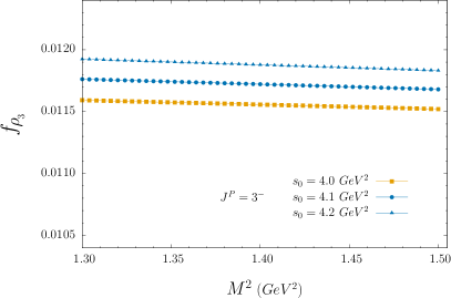
(a) The dependencies of mass and residue of the $\rho_{3}$ meson on Borel mass square $M^{2}$ at three fixed values of the continuum threshold $s_{0}$.

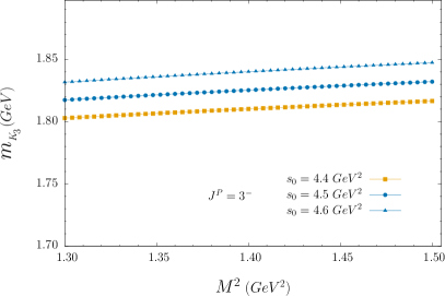
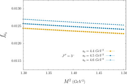
(b) The dependencies of mass and residue of the $K_{3}$ meson on Borel mass square $M^{2}$ at three fixed values of the continuum threshold $s_{0}$.

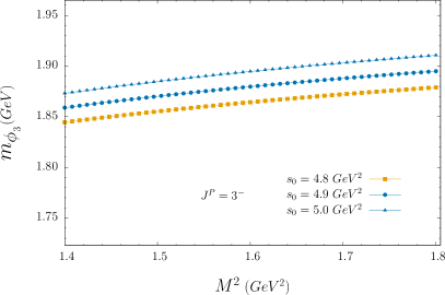
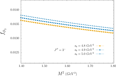
(c) The dependencies of mass and residue of the $\phi_{3}$ meson on Borel mass square $M^{2}$ at three fixed values of the continuum threshold $s_{0}$.

The continuum threshold $s_{0}$ is obtained by requiring that the variation of the masses of the $J^{P}$ tensor meson state with respect to $M^{2}$ should be minimum. Using these conditions, we determine the working regions of $s_{0}$ and $M^{2}$ for the mesons considered. These are presented in Table 1.

To show the stabilities of the working regions of $M^{2}$, in Figs. 1(a), 1(b) and 1(c), we present the dependencies of the mass and residue of $\rho_{3}(\omega_{3})$, $K_{3}$ and $\phi_{3}$ on $M^{2}$ at several fixed values of $s_{0}$. Examining these figures, we see that the values of mass and residues exhibits good stability when $M^{2}$ varies in their corresponding working regions. And, one can determine these quantities. These values are presented in Table 2. This method is denoted as Method-A in this table. Moreover, we also calculated the mass and decay constants of the $J^{P}=3^{-}$ tensor mesons with the help of the least square method (Method-B). We observe that the predictions on mass of the considered mesons of both approaches are quite close to each other.

In Table 2, we also present the experimental values of the mesons under consideration. When compared our findings with the experimental ones, we see that our results on mass values of the tensor mesons are quite compatible.

IV Conlusion

In conclusion, we have determined the mass and decay constants of the $J^{P}=3^{-}$ tensor mesons by considering the $SU(3)$ violation effects. Our predictions on the masses of the tensor mesons are in good agreement with the experimental data within the precision of the model. This finding verifies that the QCD sum rules method works quite succesfully in the analysis of the physical parameters of the higher $J$ states. The obtained decay constants can be used for further studies of the strong and electromagnetic decays of the $J^{P}=3^{-}$ tensor mesons.

References

[1]
R. Baldi, T. Bohringer, P. A. Dorsaz, V. Hungerbuhler, M. N. Kienzle-Focacci,
M. Martin, A. Mermoud, C. Nef, and P. Siegrist, “Observation of the
in the reaction at 10 GeV/c,”
Phys. Lett. B
63 (1976) 344–348.
[6]LHCb Collaboration, R. Aaij et al., “Physics case for
an LHCb Upgrade II - Opportunities in flavour physics, and beyond, in the
HL-LHC era,” [1808.08865].
[16]
K.-C. Yang, W. Y. P. Hwang, E. M. Henley, and L. S. Kisslinger, “QCD sum
rules and neutron proton mass difference,”
Phys. Rev. D 47
(1993) 3001–3012.
[18]
V. M. Belyaev and B. L. Ioffe, “Determination of the baryon mass and
baryon resonances from the quantum-chromodynamics sum rule. Strange
baryons,” Sov. Phys. JETP 57 (1983) 716–721.
[19]Particle Data Group Collaboration, R. L. Workman et al.,
“Review of Particle Physics,”
PTEP 2022 (2022)
083C01.