Implications of Pulsar Timing Array Data for Scalar-Induced Gravitational Waves and Primordial Black Holes: Primordial Non-Gaussianity $f_{\mathrm{NL}}$ Considered

Abstract

Multiple pulsar-timing-array collaborations have reported strong evidence for the existence of a gravitational-wave background. We study physical implications of this signal for cosmology, assuming that it is attributed to scalar-induced gravitational waves. By incorporating primordial non-Gaussianity $f_{\mathrm{NL}}$, we specifically examine the nature of primordial curvature perturbations and primordial black holes. We find that the signal allows for a primordial non-Gaussianity $f_{\mathrm{NL}}$ in the range of $-4.1\lesssim f_{\mathrm{NL}}\lesssim 4.1$ (68% confidence intervals) and a mass range for primordial black holes $m_{\mathrm{pbh}}$ spanning from $\sim 10^{-5}M_{\odot}$ to $\sim 10^{-2}M_{\odot}$. Furthermore, we find that the signal favors a negative non-Gaussianity, which can suppress the abundance of primordial black holes. We also demonstrate that the anisotropies of scalar-induced gravitational waves serve as a powerful tool to probe the non-Gaussianity $f_{\mathrm{NL}}$. We conduct a comprehensive analysis of the angular power spectrum within the nano-Hertz band. Looking ahead, we anticipate that future projects, such as the Square Kilometre Array, will have the potential to measure these anisotropies and provide further insights into the primordial universe.

I Introduction

Multiple collaborations in the field of PTA observations have presented strong evidence for a signal exhibiting correlations consistent with a stochastic GWB Xu et al. (2023); Antoniadis et al. (2023a); Agazie et al. (2023a); Reardon et al. (2023). The strain has been measured to be on the order of $10^{-15}$ at a pivot frequency of $1~{}\mathrm{yr}^{-1}$. Though this GWB aligns with expectations from astrophysical sources, specifically inspiraling SMBH binaries Agazie et al. (2023b), it is important to note that the current datasets do not rule out the possibility of cosmological origins or other exotic astrophysical sources, which have been explored in collaborative accompanying papers Antoniadis et al. (2023b); Afzal et al. (2023). Notably, several cosmological models have demonstrated superior fits to the signal compared to the SMBH-binary interpretation. If these alternative models are confirmed in the future, they may provide compelling evidence for new physics.

In this study, our focus lies on the cosmological interpretation of the signal, specifically the existence of SIGW Ananda et al. (2007); Baumann et al. (2007); Mollerach et al. (2004); Assadullahi and Wands (2010); Espinosa et al. (2018); Kohri and Terada (2018). This possibility had been used for interpreting the NANOGrav 12.5year dataset Arzoumanian et al. (2020) in Refs. De Luca et al. (2021); Vaskonen and Veermäe (2021); Kohri and Terada (2021); Domènech and Pi (2022); Atal et al. (2021); Yi and Fei (2023); Zhao and Wang (2023); Dandoy et al. (2023); Cai et al. (2021); Inomata et al. (2021). It was recently revisited by the PTA collaborations Antoniadis et al. (2023b); Afzal et al. (2023), but the statistics of primordial curvature perturbations was assumed to be Gaussian. However, it was demonstrated that primordial non-Gaussianity $f_{\mathrm{NL}}$ significantly contributes to the energy density of SIGW Garcia-Bellido et al. (2017); Domènech and Sasaki (2018); Cai et al. (2019); Unal (2019); Yuan and Huang (2021); Atal and Domènech (2021); Adshead et al. (2021); Ragavendra (2022); Li et al. (2023). This indicates noteworthy modifications to the energy-density spectrum, which is crucial for the data analysis of PTA datasets. On the other hand, it has been shown that primordial non-Gaussianity $f_{\mathrm{NL}}$ could generate initial inhomogeneities in SIGW, leading to anisotropies characterized by the angular power spectrum Li et al. (2023). Related studies can be found in Refs. Bartolo et al. (2020a); Valbusa Dall’Armi et al. (2021); Dimastrogiovanni et al. (2022); Schulze et al. (2023); Bartolo et al. (2022); Auclair et al. (2022); Ünal et al. (2021); Malhotra et al. (2021); Carr et al. (2021). Our analysis will encompass a comprehensive examination of the angular power spectrum within the PTA band. Moreover, this spectrum is capable of breaking the degeneracies among model parameters, particularly leading to possible determination of $f_{\mathrm{NL}}$, and playing a crucial role in distinguishing between different sources of GWB. Therefore, by interpreting the signal as originating from SIGW, we aim to study physical implications of PTA datasets for the nature of primordial curvature perturbations, including their power spectrum and angular power spectrum.

We will also study implications of the aforementioned results for scenarios involving formation of PBH, which was accompanied by the production of SIGW. Enhanced primordial curvature perturbations not only lead to formation of PBH through gravitational collapse Hawking (1971), but also produce GWB via nonlinear mode-couplings. The study of SIGW thus allows us to explore the PBH scenarios Bugaev and Klimai (2010); Saito and Yokoyama (2010); Wang et al. (2019); Kapadia et al. (2021); Chen et al. (2020); Papanikolaou (2022); Papanikolaou et al. (2021); Madge et al. (2023). Related works analyzing observational datasets can be found in Refs. Zhao and Wang (2023); Dandoy et al. (2023); Yi and Fei (2023); Afzal et al. (2023); Antoniadis et al. (2023b); Romero-Rodriguez et al. (2022); Kapadia et al. (2021), and influence of primordial non-Gaussianity on the mass function of PBH was also studied Bullock and Primack (1997); Byrnes et al. (2012); Young and Byrnes (2013); Franciolini et al. (2018); Passaglia et al. (2019); Atal and Germani (2019); Atal et al. (2019); Taoso and Urbano (2021); Meng et al. (2022); Chen et al. (2023); Kawaguchi et al. (2023); Fu et al. (2020); Inomata et al. (2021); Young et al. (2014); Choudhury et al. (2023). Taking $f_{\mathrm{NL}}$ into account in this work, we will reinterpret the constraints on power spectrum as constraints on the mass range of PBH.

The remaining context of this paper is arranged as follows. In Section II, we will provide a brief summary of the homogeneous and isotropic component of SIGW. In Section III, we will show implications of the PTA data for the power spectrum of primordial curvature perturbations and then for the mass function of PBH. In Section IV, we will study the inhomogeneous and anisotropic component of SIGW and show the corresponding angular power spectrum in PTA band. In Section V, we make concluding remarks and discussions.

II SIGW energy-density fraction spectrum

In this section, we show a brief but self-consistent summary of the main results of the energy-density fraction spectrum in a framework of SIGW theory.

For the homogeneous and isotropic component of a GWB, the energy-density fraction spectrum is defined as $\bar{\Omega}_{\mathrm{gw}}(\eta,q)=\bar{\rho}_{\mathrm{gw}}(\eta,q)/\rho_{\mathrm{crit}}(\eta)$ Maggiore (2000), where $q$ represents the wavenumber, $\rho_{\mathrm{crit}}$ denotes the critical energy density of the universe at conformal time $\eta$, and the overbar signifies quantities at the background level. This definition implies that $\int\bar{\rho}_{\mathrm{gw}}(\eta,q)\mathrm{d}\ln q$ corresponds to the energy-density fraction of GWB Maggiore (2000). The spectrum can be formally expressed as $\bar{\rho}_{\mathrm{gw}}(\eta,q)\sim\langle h_{ij,l}h_{ij,l}\rangle$, where $h_{ij}(\eta,\mathbf{q})$ represents the strain with wavevector $\mathbf{q}$, and the angle brackets denote an ensemble average. For subhorizon-scale SIGW, we have $h_{ij}\sim\zeta^{2}$, leading to $\bar{\Omega}_{\mathrm{gw}}(\eta,\mathbf{q})\sim\langle\zeta^{4}\rangle$ Ananda et al. (2007); Baumann et al. (2007), where $\zeta(\mathbf{q})$ represents curvature perturbations in the early universe. In the case of primordial Gaussianity, semi-analytic formulas for $\bar{\Omega}_{\mathrm{gw}}(\eta,\mathbf{q})$ were derived in Refs. Espinosa et al. (2018); Kohri and Terada (2018), with earlier relevant works in Refs. Ananda et al. (2007); Baumann et al. (2007). However, in the presence of primordial non-Gaussianity $f_{\mathrm{NL}}$, there are not such semi-analytic formulas. Recent literature provided relevant studies on this topic Garcia-Bellido et al. (2017); Domènech and Sasaki (2018); Cai et al. (2019); Unal (2019); Yuan and Huang (2021); Atal and Domènech (2021); Ragavendra (2022); Adshead et al. (2021); Garcia-Saenz et al. (2023); Li et al. (2023). In this work, we adopt the conventions established in our previous study Li et al. (2023).

To quantify contributions of $f_{\mathrm{NL}}$ to the energy density, we express the primordial curvature perturbations $\zeta$ in terms of their Gaussian components $\zeta_{g}$, i.e., Komatsu and Spergel (2001)

$$\zeta(\mathbf{q})=\zeta_{g}(\mathbf{q})+\frac{3}{5}f_{\mathrm{NL}}\int\frac{\mathrm{d}^{3}\mathbf{k}}{(2\pi)^{3/2}}\zeta_{g}(\mathbf{k})\zeta_{g}(\mathbf{q}-\mathbf{k})\ .$$ (1)

Here, $f_{\mathrm{NL}}$ represents the non-linear parameter that characterizes the local-type primordial non-Gaussianity. To simplify the subsequent analytic formulae, we introduce a new quantity as follows

$$F_{\mathrm{NL}}=\frac{3}{5}f_{\mathrm{NL}}\ .$$ (2)

It is worth noting that perturbation theory requires the condition $A_{S}F_{\mathrm{NL}}^{2}<1$, where $A_{S}$ will be defined later. We define the dimensionless power spectrum of $\zeta_{g}$ as

$$\langle\zeta_{g}(\mathbf{q})\zeta_{g}(\mathbf{q}^{\prime})\rangle=\delta^{(3)}(\mathbf{q}+\mathbf{q}^{\prime})\frac{2\pi^{2}}{q^{3}}\Delta^{2}_{g}(q)\ .$$ (3)

In this work, we assume that $\Delta^{2}_{g}(q)$ follows a log-normal distribution with respect to $\ln q$ Pi and Sasaki (2020); Adshead et al. (2021); Zhao and Wang (2023); Dimastrogiovanni et al. (2023); Cang et al. (2023)

$$\Delta^{2}_{g}(q)=\frac{A_{S}}{\sqrt{2\pi\sigma^{2}}}\exp\left[-\frac{\ln^{2}(q/q_{\ast})}{2\sigma^{2}}\right]\ ,$$ (4)

where $A_{S}$ represents the spectral amplitude at the spectral peak wavenumber $q_{\ast}$, and $\sigma$ denotes the standard deviation that characterizes the width of the spectrum. The wavenumber $q$ is straightforwardly converted into the frequency $\nu$, namely, $q=2\pi\nu$.

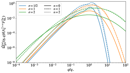
Figure 1: Unscaled (or equivalently, $A_{S}=1$ and $F_{\mathrm{NL}}=1$) contributions to the energy-density fraction spectrum of SIGW. We display $\sigma=1/2,1,2$ and produce this figure by using the original data of Ref. Li et al. (2023).

Through a detailed derivation process based on Wick’s theorem, we can decompose $\bar{\Omega}_{\mathrm{gw}}\sim\langle\zeta^{4}\rangle$ into three components depending on the power of $f_{\mathrm{NL}}$. However, the complete derivations have been simplified by employing a Feynman-like diagrammatic approach Garcia-Bellido et al. (2017); Unal (2019); Atal and Domènech (2021); Ragavendra (2022); Adshead et al. (2021); Li et al. (2023). Here, we present the final results

$$\bar{\Omega}_{\mathrm{gw}}(\eta,q)=\bar{\Omega}_{\mathrm{gw}}^{(0)}(\eta,q)+\bar{\Omega}_{\mathrm{gw}}^{(1)}(\eta,q)+\bar{\Omega}_{\mathrm{gw}}^{(2)}(\eta,q)\ .$$ (5)

where we provide the analytic expressions for $\bar{\Omega}_{\mathrm{gw}}^{(n)}$, which are proportional to $A_{S}^{2}(A_{S}F_{\mathrm{NL}}^{2})^{n}$ with $n=0,1,2$, in Appendix A. They were evaluated using the vegas package Lepage (2021), while their numerical results for $\sigma=1/2,1,2$ are reproduced in Fig. 1. Specifically, $\bar{\Omega}_{\mathrm{gw}}^{(0)}$ corresponds to the energy-density fraction spectrum in the case of Gaussianity, while $\bar{\Omega}_{\mathrm{gw}}^{(1)}$ and $\bar{\Omega}_{\mathrm{gw}}^{(2)}$ fully describe the contributions of local-type primordial non-Gaussianity $f_{\mathrm{NL}}$.

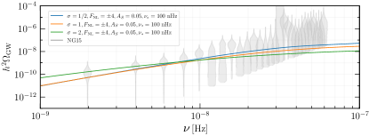
Figure 2: Energy-density fraction spectra of SIGW for different sets of independent parameters. The NG15 data are also shown for comparison.

The energy-density fraction spectrum of SIGW at the present conformal time $\eta_{0}$ can be expressed as

$$\bar{\Omega}_{\mathrm{gw},0}(\nu)=\Omega_{\mathrm{rad},0}\left[\frac{g_{\ast,\rho}(T)}{g_{\ast,\rho}(T_{\mathrm{eq}})}\right]\left[\frac{g_{\ast,s}(T_{\mathrm{eq}})}{g_{\ast,s}(T)}\right]^{4/3}\bar{\Omega}_{\mathrm{gw}}(\eta,q)\ .$$ (6)

In the above equation, $\Omega_{\mathrm{rad},0}h^{2}=4.2\times 10^{-5}$ represents the physical energy-density fraction of radiations in the present universe Aghanim et al. (2020). $T$ and $T_{\mathrm{eq}}$ correspond to the cosmic temperatures at the emission time and the epoch of matter-radiation equality, respectively. $\nu$ can be related to $T$, $g_{\ast,\rho}(T)$, and $g_{\ast,s}(T)$ as follows Zhao and Wang (2023)

$$\frac{\nu}{\mathrm{nHz}}=26.5\left(\frac{T}{\mathrm{GeV}}\right)\left(\frac{g_{\ast,\rho}(T)}{106.75}\right)^{1/2}\left(\frac{g_{\ast,s}(T)}{106.75}\right)^{-1/3}\ .$$ (7)

Here, $g_{\ast,\rho}$ and $g_{\ast,s}$ represent the effective relativistic degrees of freedom in the universe, which are tabulated functions of $T$ as provided in Ref. Saikawa and Shirai (2018). To illustrate the interpretation of current PTA data in the framework of SIGW, we depict $\bar{\Omega}_{\mathrm{gw},0}(\nu)$ with respect to $\nu$ in Fig. 2, using three specific sets of model parameters.

III Implications of PTA data for new physics

In this section, we investigate the potential constraints on the parameter space of the primordial power spectrum and PBH using the NG15 data. While it is possible to obtain constraints from other PTA datasets using the same methodology, we do not consider them in this study, as they would not significantly alter the leading results of our current work.

By performing a comprehensive Bayesian analysis Afzal et al. (2023), we could gain valuable insights for the posteriors of four independent parameters, i.e., $F_{\mathrm{NL}}$, $A_{S}$, $\sigma$, and $\nu_{\ast}$, for which the priors are set to be $F_{\mathrm{NL}}\in[-30,30]$, $\log_{10}A_{S}\in[-3,1]$, $\sigma\in[0,5]$, and $\log_{10}(\nu_{\ast}/\mathrm{Hz})\in[-9,-5]$. Here, we also adopt the aforementioned condition of perturbativity, namely, $A_{S}F_{\mathrm{NL}}^{2}<1$. The inference results within 68% confidence intervals are given as

$$F_{\mathrm{NL}} = -0.00^{+2.45}_{-2.46}\ ,$$ (8)

$$\log_{10}A_{S} = -0.97^{+0.65}_{-0.46}\ ,$$ (9)

$$\sigma = 1.08^{+1.08}_{-0.83}\ ,$$ (10)

$$\log_{10}(\nu_{\ast}/\mathrm{Hz}) = -6.99^{+0.93}_{-0.45}\ .$$ (11)

We can also recast Eq. (8) into constraints on $f_{\mathrm{NL}}$, i.e.,

$$f_{\mathrm{NL}}=-0.0\pm 4.1\ .$$ (12)

Fig. 3 shows two-dimensional contours in $\log_{10}A_{S}-F_{\mathrm{NL}}$ plane at 68% (dark blue regions) and 95% (light blue regions) confidence levels. There is a full degeneracy in the sign of primordial non-Gaussianity $f_{\mathrm{NL}}$, as the energy-density fraction spectrum is dependent of only the absolute value of $F_{\mathrm{NL}}$, as demonstrated in Fig. 1. The above results indicate that the PTA observations have already emerged as a powerful tool for probing physics of the early universe.

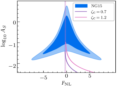
Figure 3: Two-dimensional contours (blue shaded) in $\log_{10}A_{S}-F_{\mathrm{NL}}$ plane inferred from the NG15 data. Dotted lines denote $F_{\mathrm{NL}}=-(4\zeta_{c})^{-1}$ while solid curves stand for models, which expect $f_{\mathrm{pbh}}=1$ for $m_{\mathrm{pbh}}=10^{-2}M_{\odot}$, in the cases of $\zeta_{c}=0.7$ (purple) and $\zeta_{c}=1.2$ (rose), respectively.

We can further recast the constraints on the primordial curvature power spectrum into constraints on the nature of PBH, which is characterized by their mass function. Due to significant uncertainties in the formation scenarios of PBH (as discussed in reviews such as Ref. Carr et al. (2021)), we adopt a simplified scenario Meng et al. (2022) to illustrate the importance of primordial non-Gaussianity $f_{\mathrm{NL}}$. The initial mass function of PBH is described by

$$\beta=\int_{\zeta>\zeta_{c}}P(\zeta)d\zeta=\int_{\zeta(\zeta_{g})>\zeta_{c}}\frac{1}{\sqrt{2\pi}\sigma_{g}}\mathrm{exp}\left(-\frac{\zeta_{g}^{2}}{2\sigma_{g}^{2}}\right)d\zeta_{g}\ ,$$ (13)

where $P(\zeta)$ represents the PDF of primordial curvature perturbations, $\sigma_{g}$ is the standard variance of the Gaussian component $\zeta_{g}$ in the PDF, and $\zeta_{c}$ stands for the critical fluctuation. We further find $\sigma_{g}^{2}=\langle\zeta_{g}^{2}\rangle=\int\Delta_{g}^{2}(q)d\ln q=A_{S}$ by considering the power spectrum defined in Eq. (4). Additionally, it is known that $\zeta_{c}$ is of order $\mathcal{O}(1)$, with specific values of $0.7$ and $1.2$, as suggested by Ref. Green et al. (2004).

To evaluate Eq. (13), we devide $F_{\mathrm{NL}}$ into two regimes, i.e., $F_{\mathrm{NL}}>0$ and $F_{\mathrm{NL}}<0$. In the case of $F_{\mathrm{NL}}>0$, we solve the equation $\zeta(\zeta_{g})=\zeta_{c}$, yielding a relation

$$\zeta_{g\pm}=\frac{-1\pm\sqrt{1+4F_{\mathrm{NL}}\zeta_{c}}}{2F_{\mathrm{NL}}}\ .$$ (14)

By substituting it into Eq. (13), we gain

$$\beta = \left(\int_{-\infty}^{\zeta_{g-}}+\int^{+\infty}_{\zeta_{g+}}\right)P(\zeta_{g})d\zeta_{g}$$ (15)

$$= \frac{1}{2}\mathrm{erfc}\left(\frac{\zeta_{g+}}{\sqrt{2A_{S}}}\right)+\frac{1}{2}\mathrm{erfc}\left(-\frac{\zeta_{g-}}{\sqrt{2A_{S}}}\right)\ ,$$

where erfc(x) is the complementary error function. Similarly, in the case of $-(4\zeta_{c})^{-1}<F_{\mathrm{NL}}<0$, we gain

$$\beta=\int_{\zeta_{g+}}^{\zeta_{g-}}P(\zeta_{g})d\zeta_{g}=\frac{1}{2}\mathrm{erfc}\left(\frac{\zeta_{g+}}{\sqrt{2A_{S}}}\right)-\frac{1}{2}\mathrm{erfc}\left(\frac{\zeta_{g-}}{\sqrt{2A_{S}}}\right)\ .$$ (16)

In contrast, in the case of $F_{\mathrm{NL}}<-(4\zeta_{c})^{-1}$, no PBH were formed in the early universe, since the curvature perturbations are expected to never exceed the critical fluctuation. As a viable candidate for cold dark matter, the abundance of PBH is determined as Nakama et al. (2017)

$$f_{\mathrm{pbh}}\simeq 2.5\times 10^{8}\beta\left(\frac{g_{\ast,\rho}(T_{\mathrm{f}})}{10.75}\right)^{-1/4}\left(\frac{m_{\mathrm{pbh}}}{M_{\odot}}\right)^{-1/2}\ ,$$ (17)

where $m_{\mathrm{pbh}}$ represents the mass of PBH, and $T_{\mathrm{f}}$ denotes cosmic temperature at the formation occasion. Roughly speaking, $m_{\mathrm{pbh}}$ can be related to the horizon mass $m_{H}$ and then the peak frequency $\nu_{\ast}$, namely, Kohri and Terada (2021)

$$\frac{m_{\mathrm{pbh}}}{M_{\odot}}\simeq\frac{m_{H}}{0.31M_{\odot}}\simeq\left(\frac{\nu_{\ast}}{5.0\mathrm{nHz}}\right)^{-2}\ .$$ (18)

Based on Eq. (11), we could infer that the mass range of PBH is the order of $\mathcal{O}(10^{-5}-10^{-2})M_{\odot}$. However, the inferred abundance of PBH exceeds unity in the case of a sizable positive $F_{\mathrm{NL}}$, indicating an overproduction of PBH. This is because the inferred value of $A_{S}$ is typically one order of magnitude larger than the value of $A_{S}$ that leads to $f_{\mathrm{pbh}}=1$. To illustrate this result more clearly, we include into Fig. 3 two solid curves corresponding to $m_{\mathrm{pbh}}=10^{-2}M_{\odot}$ and $f_{\mathrm{pbh}}=1$ in the cases of $\zeta_{c}=0.7$ (purple curve) and $\zeta_{c}=1.2$ (rose curve), respectively. For comparison, we mark the critical value $F_{\mathrm{NL}}=-(4\zeta_{c})^{-1}$ with dotted lines. Therefore, we find that a negative $F_{\mathrm{NL}}$ is capable of alleviating the overproduction of PBH, especially when considering a sizable negative $F_{\mathrm{NL}}$, namely, $F_{\mathrm{NL}}<-(4\zeta_{c})^{-1}$, which prevents the formation of any PBH. However, due to large uncertainties in model buildings, it remains challenging to exclude the PBH scenario through analyzing the present PTA data.

In summary, it is crucial to measure the primordial non-Gaussianity or at least determine the sign of $F_{\mathrm{NL}}$ in order to assess the viability of the PBH scenario. However, it is impossible to determine the sign of $F_{\mathrm{NL}}$ through measurements of the energy-density fraction spectrum of SIGW, due to the sign degeneracy. In the next section, we will propose that the inhomogeneous and anisotropic component of SIGW has the potential to break the sign degeneracy, as well as other degeneracies in model parameters, opening up new possibilities for making judgments about the PBH scenario in the future.

IV SIGW angular power spectrum

In this section, we investigate the inhomogeneities and anisotropies in SIGW via deriving the angular power spectrum in the PTA band, following the research approach established in our previous paper Li et al. (2023).

The inhomogeneities in SIGW arise from the long-wavelength modulations of the energy density generated by short-wavelength modes. As discussed in Section II, SIGW originate from extremely high redshifts, corresponding to very small horizons. However, due to limitations in the angular resolution of detectors, the signal along a line-of-sight represents an ensemble average of the energy densities over a sizable number of such horizons. Consequently, any two signals would appear identical. Nevertheless, the energy density of SIGW produced by short-wavelength modes can be spatially redistributed by long-wavelength modes if there are couplings between the two. The local-type primordial non-Gaussianity $f_{\mathrm{NL}}$ could contribute to such couplings.

Similar to the temperature fluctuations of relic photons Seljak and Zaldarriaga (1996), the initial inhomogeneities in SIGW at a spatial location $\mathbf{x}$ can be characterized by the density contrast, which is denoted as $\delta_{\mathrm{gw}}(\eta,\mathbf{x},\mathbf{q})$, given by

$$\delta_{\mathrm{gw}}(\eta,\mathbf{x},\mathbf{q})=4\pi\frac{\omega_{\mathrm{gw}}(\eta,\mathbf{x},\mathbf{q})}{\bar{\Omega}_{\mathrm{gw}}(\eta,q)}-1,$$ (19)

where the energy-density full spectrum $\omega_{\mathrm{gw}}(\eta,\mathbf{x},\mathbf{q})$ is defined in terms of the energy density, namely, $\rho_{\mathrm{gw}}(\eta,\mathbf{x})=\rho_{\mathrm{crit}}(\eta)\int\mathrm{d}^{3}\mathbf{q},\omega_{\mathrm{gw}}(\eta,\mathbf{x},\mathbf{q})/q^{3}$. We specifically get $\omega_{\mathrm{gw}}\sim\langle\zeta^{4}\rangle_{\mathbf{x}}$, where the subscript _x denotes an ensemble average within the horizon enclosing $\mathbf{x}$ Bartolo et al. (2020a); Li et al. (2023). We decompose $\zeta_{g}$ into modes of short-wavelength $\zeta_{gS}$ and long-wavelength $\zeta_{gL}$, namely, $\zeta_{g}=\zeta_{gS}+\zeta_{gL}$ Tada and Yokoyama (2015). At linear order in $\zeta_{gL}$, we get $\delta_{\mathrm{gw}}\sim\zeta_{gL}\langle\zeta_{gS}\zeta_{S}^{3}\rangle_{\mathbf{x}}$, where $\zeta_{S}$ represents the part of $\zeta$ composed solely of $\zeta_{gS}$. Terms of higher orders in $\zeta_{gL}$ are negligible due to smallness of the power spectrum $\Delta_{L}^{2}\sim 10^{-9}$ Aghanim et al. (2020). Using Feynman-like rules and diagrams, we get an expression for $\delta_{\mathrm{gw}}(\eta,\mathbf{x},\mathbf{q})$, i.e., Li et al. (2023)

$$\delta_{\mathrm{gw}}(\eta,\mathbf{x},\mathbf{q})=F_{\mathrm{NL}}\frac{\Omega_{\mathrm{ng}}(\eta,q)}{\bar{\Omega}_{\mathrm{gw}}(\eta,q)}\int\frac{d^{3}\mathbf{k}}{(2\pi)^{3/2}}e^{i\mathbf{k}\cdot\mathbf{x}}\zeta_{gL}(\mathbf{k})\ ,$$ (20)

where we introduce a quantity of the form

$$\Omega_{\mathrm{ng}}(\eta,q)=2^{3}\bar{\Omega}_{\mathrm{gw}}^{(0)}(\eta,q)+2^{2}\bar{\Omega}_{\mathrm{gw}}^{(1)}(\eta,q)\ .$$ (21)

The present density contrast, denoted as $\delta_{\mathrm{gw},0}(\mathbf{q})$, can be estimated analytically using the line-of-sight approach Contaldi (2017); Bartolo et al. (2019, 2020b). It is contributed by both the initial inhomogeneities and propagation effects, given by Bartolo et al. (2020a)

$$\delta_{\mathrm{gw},0}(\mathbf{q})=\delta_{\mathrm{gw}}(\eta,\mathbf{x},\mathbf{q})+\left[4-n_{\mathrm{gw},0}(\nu)\right]\Phi(\eta,\mathbf{x})\ .$$ (22)

Here, $n_{\mathrm{gw},0}(\mathbf{q})$ denotes the index of the present energy-density fraction spectrum in Eq. (6), given by

$$n_{\mathrm{gw},0}(\nu)=\frac{\partial\ln\bar{\Omega}_{\mathrm{gw},0}(\nu)}{\partial\ln\nu}\simeq\frac{\partial\ln\bar{\Omega}_{\mathrm{gw}}(\eta,q)}{\partial\ln q}\Big{|}_{q=2\pi\nu}\ .$$ (23)

For the propagation effects, we consider only the SW effect Sachs and Wolfe (1967), which is characterized by the Bardeen’s potential on large scales

$$\Phi(\eta,\mathbf{x})=\frac{3}{5}\int\frac{d^{3}\mathbf{k}}{(2\pi)^{3/2}}e^{i\mathbf{k}\cdot\mathbf{x}}\zeta_{gL}(\mathbf{k})\ .$$ (24)

We assume the statistical homogeneity and isotropy for the density contrasts on large scales, similar to the study of CMB Maggiore (2018).

The anisotropies today can be mapped from the aforementioned inhomogeneities. The reduced angular power spectrum is useful to characterize the statistics of these anisotropies. It is defined as the two-point correlator of the present density contrast, namely,

$$\langle\delta_{\mathrm{gw},0,\ell m}(2\pi\nu)\delta_{\mathrm{gw},0,\ell^{\prime}m^{\prime}}^{\ast}(2\pi\nu)\rangle=\delta_{\ell\ell^{\prime}}\delta_{mm^{\prime}}\widetilde{C}_{\ell}(\nu)\ ,$$ (25)

where $\delta_{\mathrm{gw},0}(\mathbf{q})$ has been expanded in terms of spherical harmonics, i.e.,

$$\delta_{\mathrm{gw},0}(\mathbf{q})=\sum_{\ell m}\delta_{\mathrm{gw},0,\ell m}(q)Y_{\ell m}(\mathbf{n})\ .$$ (26)

Roughly speaking, we get $\widetilde{C}_{\ell}\sim\delta_{\mathrm{gw},0}^{2}\propto\langle\zeta_{gL}\zeta_{gL}\rangle\sim\Delta_{L}^{2}$. Detailed analysis using Feynman-like rules and diagrams was conducted in our previous paper Li et al. (2023). We summarize the main results as follows

$$\widetilde{C}_{\ell}(\nu)=\frac{18\pi\Delta^{2}_{L}}{25\ell(\ell+1)}\biggl{\{}f_{\mathrm{NL}}\frac{\Omega_{\mathrm{ng}}(\eta,2\pi\nu)}{\bar{\Omega}_{\mathrm{gw}}(\eta,2\pi\nu)}+\bigl{[}4-n_{\mathrm{gw},0}(\nu)\bigr{]}\biggr{\}}^{2}\ ,$$ (27)

which can be recast into the angular power spectrum

$$C_{\ell}(\nu)=\left[\frac{\bar{\Omega}_{\mathrm{gw},0}(\nu)}{4\pi}\right]^{2}\tilde{C}{\ell}(\nu)\ .$$ (28)

Analogous to CMB, for which the root-mean-square (rms) temperature fluctuations is determined by $[{\ell(\ell+1)C^{\mathrm{CMB}}_{\ell}/(2\pi)}]^{1/2}$, the rms density contrast for SIGW is determined by $[{\ell(\ell+1)C_{\ell}(\nu)/(2\pi)}]^{1/2}$, which represents the variance of the energy-density fluctuations. It is vital to note that the rms density contrast is constant with respect to multipoles $\ell$, but depends on frequency bands.

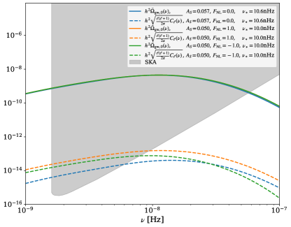
Figure 4: Physical energy-density fraction spectra of SIGWs, $h^{2}\Omega_{\mathrm{gw},0}(\nu)$ (solid), and the variance of SIGW density contrasts, $h^{2}[{\ell(\ell+1)C_{\ell}(\nu)/(2\pi)}]^{1/2}$ (dashed). For comparison, we show the sensitivity region of SKA Schmitz (2021) (gray shaded).

In Figure 4, we present the rms density contrast as a function of gravitational-wave frequency. We also include the energy-density fraction spectrum for comparison. Roughly speaking, we find that $\sqrt{\tilde{C}_{\ell}}$ is the order of $10^{-4}$, depending on specific sets of model parameters. It is worth noting that the angular power spectrum can break degeneracies among these parameters. For instance, based on Fig. 4, we observe a coincidence in the energy-density fraction spectra for three different parameter sets. However, the angular power spectrum breaks this coincidence, particularly in the case of the sign degeneracy of $f_{\mathrm{NL}}$. This result suggests that measurements of the anisotropies in SIGW have the potential to determine the primordial non-Gaussianity Li et al. (2023). Recently, an upper limit of $\tilde{C}_{\ell}<20\%$ was inferred from the NG15 data Agazie et al. (2023c). However, this limit is not precise enough to test the theoretical predictions of our present work. In contrast, based on Fig. 4, we anticipate that the SKA program Schmitz (2021) will offer sufficient precision to measure the non-Gaussianity $f_{\mathrm{NL}}$.

V Conclusions

In this study, we examined the implications of recent PTA datasets for understanding the nature of primordial curvature perturbations and primordial black holes (PBH). Specifically, we investigated the influence of primordial non-Gaussianity $f_{\mathrm{NL}}$ on the inference of model parameters, and vice versa, by analyzing the recent NG15 data. In particular, at 68% confidence level, we inferred $|f_{\mathrm{NL}}|<4.1$, which is competitive with the constraints from measurements of CMB. Even when considering the non-Gaussianity $f_{\mathrm{NL}}$, we found that the PBH scenario is in tension with the NG15 data, except when a sizable negative $f_{\mathrm{NL}}$ is considered, which can significantly suppress the abundance of PBH. Our results indicated that the PTA observations have already emerged as a powerful tool for probing physics of the early universe and dark matter. Moreover, we proposed that the anisotropies of SIGW serve as a powerful probe of the non-Gaussianity $f_{\mathrm{NL}}$ in the PTA band. For the first time, we conducted the complete analysis of the angular power spectrum in this frequency band and found that it can effectively break potential degeneracies among the model parameters, particularly the sign degeneracy of $f_{\mathrm{NL}}$. Additionally, we explored the detectability of the anisotropies in SIGW in the era of the SKA project.

Notes added.— During the preparation of this paper, a related study Franciolini et al. (2023) appears, which examines the posteriors of NG15 data. The authors suggest that the Gaussian scenarios for SIGW are in tension with the current PTA data at a $2\sigma$ confidence level, but non-Gaussian scenarios that suppress the abundance of PBH can alleviate this tension. Given the significant uncertainties in the formation scenarios of PBH (as discussed in reviews such as Ref. Carr et al. (2021)), the main focus of our research is to simultaneously examine the energy-density fraction spectrum and the angular power spectrum of SIGW, by incorporating the complete contributions arising from primordial non-Gaussianity $f_{\mathrm{NL}}$. We also address the importance of primordial non-Gaussianity to SIGW through a Bayesian analysis over the NG15 data.

Appendix A Formulae for evaluating the SIGW energy density

After a comprehensive derivation following the methodology presented in Refs. Adshead et al. (2021); Li et al. (2023); Ragavendra (2022), we can precisely express the three terms in Eq. (5) as

$$\bar{\Omega}_{\mathrm{gw}}^{(0)}(\eta,q) = \frac{1}{3}\int_{0}^{\infty}\mathrm{d}t_{1}\int_{-1}^{1}\mathrm{d}s_{1}\mkern 1.5mu\overline{\mkern-1.5muJ^{2}(u_{1},v_{1},x\rightarrow\infty)\mkern-1.5mu}\mkern 1.5mu\frac{1}{(u_{1}v_{1})^{2}}\Delta^{2}_{g}(v_{1}q)\Delta^{2}_{g}(u_{1}q)\ ,$$ (29)

$$\bar{\Omega}_{\mathrm{gw}}^{(1)}(\eta,q) = \frac{F_{\mathrm{NL}}^{2}}{3\pi}\prod_{i=1}^{2}\biggl{[}\int_{0}^{\infty}\mathrm{d}t_{i}\int_{-1}^{1}\mathrm{d}s_{i}\,v_{i}u_{i}\biggr{]}\Bigg{\{}\frac{\pi\mkern 1.5mu\overline{\mkern-1.5muJ^{2}(u_{1},v_{1},x\rightarrow\infty)\mkern-1.5mu}\mkern 1.5mu}{(u_{1}v_{1}u_{2}v_{2})^{3}}\Delta^{2}_{g}(v_{1}v_{2}q)\Delta^{2}_{g}(u_{1}q)\Delta^{2}_{g}(v_{1}u_{2}q)$$

$$\qquad+\int_{0}^{2\pi}\mathrm{d}\varphi_{12}\,\cos 2\varphi_{12}\mkern 1.5mu\overline{\mkern-1.5muJ(u_{1},v_{1},x\rightarrow\infty)J(u_{2},v_{2},x\rightarrow\infty)\mkern-1.5mu}\mkern 1.5mu$$

$$\hphantom{\qquad\ +\int_{0}^{2\pi}\mathrm{d}\varphi_{12}}\times\frac{\Delta^{2}_{g}(v_{2}q)}{v_{2}^{3}}\frac{\Delta^{2}_{g}(w_{12}q)}{w_{12}^{3}}\bigg{[}\frac{\Delta^{2}_{g}(u_{2}q)}{u_{2}^{3}}+\frac{\Delta^{2}_{g}(u_{1}q)}{u_{1}^{3}}\bigg{]}\Bigg{\}}\ ,$$

$$\bar{\Omega}_{\mathrm{gw}}^{(2)}(\eta,q) = \frac{F_{\mathrm{NL}}^{4}}{24\pi^{2}}\prod_{i=1}^{3}\biggl{[}\int_{0}^{\infty}\mathrm{d}t_{i}\int_{-1}^{1}\mathrm{d}s_{i}\,v_{i}u_{i}\biggr{]}\Bigg{\{}\frac{2\pi^{2}\mkern 1.5mu\overline{\mkern-1.5muJ^{2}(u_{1},v_{1},x\rightarrow\infty)\mkern-1.5mu}\mkern 1.5mu}{(u_{1}v_{1}u_{2}v_{2}u_{3}v_{3})^{3}}\Delta^{2}_{g}(v_{1}v_{2}q)\Delta^{2}_{g}(v_{1}u_{2}q)\Delta^{2}_{g}(u_{1}v_{3}q)\Delta^{2}_{g}(u_{1}u_{3}q)$$

$$\qquad\ +\int_{0}^{2\pi}\mathrm{d}\varphi_{12}\mathrm{d}\varphi_{23}\,\cos 2\varphi_{12}\mkern 1.5mu\overline{\mkern-1.5muJ(u_{1},v_{1},x\rightarrow\infty)J(u_{2},v_{2},x\rightarrow\infty)\mkern-1.5mu}\mkern 1.5mu$$

$$\hphantom{\qquad\ +\int_{0}^{2\pi}\mathrm{d}\varphi_{12}\mathrm{d}\varphi_{23}\,}\times\frac{\Delta^{2}_{g}(u_{3}q)}{u_{3}^{3}}\frac{\Delta^{2}_{g}(w_{13}q)}{w_{13}^{3}}\bigg{[}\frac{\Delta^{2}_{g}(v_{3}q)}{v_{3}^{3}}\frac{\Delta^{2}_{g}(w_{23}q)}{w_{23}^{3}}+\frac{\Delta^{2}_{g}(w_{23}q)}{w_{23}^{3}}\frac{\Delta^{2}_{g}(w_{123}q)}{w_{123}^{3}}\bigg{]}\Bigg{\}}\ ,$$

where we define $x=q\eta$, $s_{i}=u_{i}-v_{i}$, $t_{i}=u_{i}+v_{i}-1$, and

$$y_{ij} = \frac{\cos\varphi_{ij}}{4}\sqrt{t_{i}(t_{i}+2)(1-s_{i}^{2})t_{j}(t_{j}+2)(1-s_{j}^{2})}+\frac{1}{4}[1-s_{i}(t_{i}+1)][1-s_{j}(t_{j}+1)]\ ,$$ (32a)

$$w_{ij} = \sqrt{v_{i}^{2}+v_{j}^{2}-y_{ij}}\ ,$$ (32b)

$$w_{123} = \sqrt{v_{1}^{2}+v_{2}^{2}+v_{3}^{2}+y_{12}-y_{13}-y_{23}}\ .$$ (32c)

The calculation for the average of the squared oscillation $J(u,v,x\rightarrow\infty)$ has been provided in Ref. Li et al. (2023), as well as in earlier studies referenced in Refs. Espinosa et al. (2018); Kohri and Terada (2018); Atal and Domènech (2021); Adshead et al. (2021), i.e.,

$$\mkern 1.5mu\overline{\mkern-1.5muJ(u_{i},v_{i},x\rightarrow\infty)J(u_{j},v_{j},x\rightarrow\infty)\mkern-1.5mu}\mkern 1.5mu$$

$$= \frac{9\left(1-s_{i}^{2}\right)\left(1-s_{j}^{2}\right)t_{i}\left(t_{i}+2\right)t_{j}\left(t_{j}+2\right)\left(s_{i}^{2}+t_{i}^{2}+2t_{i}-5\right)\left(s_{j}^{2}+t_{j}^{2}+2t_{j}-5\right)}{8\left(-s_{i}+t_{i}+1\right){}^{3}\left(s_{i}+t_{i}+1\right){}^{3}\left(-s_{j}+t_{j}+1\right){}^{3}\left(s_{j}+t_{j}+1\right){}^{3}}$$

$$\times\Bigg{\{}\left[\left(s_{i}^{2}+t_{i}^{2}+2t_{i}-5\right)\ln\left(\left|\frac{t_{i}^{2}+2t_{i}-2}{s_{i}^{2}-3}\right|\right)+2\left(s_{i}-t_{i}-1\right)\left(s_{i}+t_{i}+1\right)\right]$$

$$\hphantom{\times\Bigg{\{}}\times\left[\left(s_{j}^{2}+t_{j}^{2}+2t_{j}-5\right)\ln\left(\left|\frac{t_{j}^{2}+2t_{j}-2}{s_{j}^{2}-3}\right|\right)+2\left(s_{j}-t_{j}-1\right)\left(s_{j}+t_{j}+1\right)\right]$$

$$\hphantom{\times\Bigg{\{}}+\pi^{2}\Theta\left(t_{i}-\sqrt{3}+1\right)\Theta\left(t_{j}-\sqrt{3}+1\right)\left(s_{i}^{2}+t_{i}^{2}+2t_{i}-5\right)\left(s_{j}^{2}+t_{j}^{2}+2t_{j}-5\right)\Bigg{\}}\ .$$

The equations presented in this appendix can be utilized to numerically calculate the energy density of SIGW in a self-consistent manner.

References

- Xu et al. (2023) H. Xu et al., Res. Astron. Astrophys. 23, 075024 (2023), arXiv:2306.16216 [astro-ph.HE] .
- Antoniadis et al. (2023a) J. Antoniadis et al., (2023a), arXiv:2306.16214 [astro-ph.HE] .
- Agazie et al. (2023a) G. Agazie et al. (NANOGrav), Astrophys. J. Lett. 951 (2023a), 10.3847/2041-8213/acdac6, arXiv:2306.16213 [astro-ph.HE] .
- Reardon et al. (2023) D. J. Reardon et al., Astrophys. J. Lett. 951 (2023), 10.3847/2041-8213/acdd02, arXiv:2306.16215 [astro-ph.HE] .
- Agazie et al. (2023b) G. Agazie et al. (NANOGrav), (2023b), arXiv:2306.16220 [astro-ph.HE] .
- Antoniadis et al. (2023b) J. Antoniadis et al., (2023b), arXiv:2306.16227 [astro-ph.CO] .
- Afzal et al. (2023) A. Afzal et al. (NANOGrav), Astrophys. J. Lett. 951 (2023), 10.3847/2041-8213/acdc91, arXiv:2306.16219 [astro-ph.HE] .
- Ananda et al. (2007) K. N. Ananda, C. Clarkson, and D. Wands, Phys. Rev. D 75, 123518 (2007), arXiv:gr-qc/0612013 .
- Baumann et al. (2007) D. Baumann, P. J. Steinhardt, K. Takahashi, and K. Ichiki, Phys. Rev. D 76, 084019 (2007), arXiv:hep-th/0703290 .
- Mollerach et al. (2004) S. Mollerach, D. Harari, and S. Matarrese, Phys. Rev. D 69, 063002 (2004), arXiv:astro-ph/0310711 .
- Assadullahi and Wands (2010) H. Assadullahi and D. Wands, Phys. Rev. D 81, 023527 (2010), arXiv:0907.4073 [astro-ph.CO] .
- Espinosa et al. (2018) J. R. Espinosa, D. Racco, and A. Riotto, JCAP 09, 012 (2018), arXiv:1804.07732 [hep-ph] .
- Kohri and Terada (2018) K. Kohri and T. Terada, Phys. Rev. D 97, 123532 (2018), arXiv:1804.08577 [gr-qc] .
- Arzoumanian et al. (2020) Z. Arzoumanian et al. (NANOGrav), Astrophys. J. Lett. 905, L34 (2020), arXiv:2009.04496 [astro-ph.HE] .
- De Luca et al. (2021) V. De Luca, G. Franciolini, and A. Riotto, Phys. Rev. Lett. 126, 041303 (2021), arXiv:2009.08268 [astro-ph.CO] .
- Vaskonen and Veermäe (2021) V. Vaskonen and H. Veermäe, Phys. Rev. Lett. 126, 051303 (2021), arXiv:2009.07832 [astro-ph.CO] .
- Kohri and Terada (2021) K. Kohri and T. Terada, Phys. Lett. B 813, 136040 (2021), arXiv:2009.11853 [astro-ph.CO] .
- Domènech and Pi (2022) G. Domènech and S. Pi, Sci. China Phys. Mech. Astron. 65, 230411 (2022), arXiv:2010.03976 [astro-ph.CO] .
- Atal et al. (2021) V. Atal, A. Sanglas, and N. Triantafyllou, JCAP 06, 022 (2021), arXiv:2012.14721 [astro-ph.CO] .
- Yi and Fei (2023) Z. Yi and Q. Fei, Eur. Phys. J. C 83, 82 (2023), arXiv:2210.03641 [astro-ph.CO] .
- Zhao and Wang (2023) Z.-C. Zhao and S. Wang, Universe 9, 157 (2023), arXiv:2211.09450 [astro-ph.CO] .
- Dandoy et al. (2023) V. Dandoy, V. Domcke, and F. Rompineve, (2023), arXiv:2302.07901 [astro-ph.CO] .
- Cai et al. (2021) R.-G. Cai, C. Chen, and C. Fu, Phys. Rev. D 104, 083537 (2021), arXiv:2108.03422 [astro-ph.CO] .
- Inomata et al. (2021) K. Inomata, M. Kawasaki, K. Mukaida, and T. T. Yanagida, Phys. Rev. Lett. 126, 131301 (2021), arXiv:2011.01270 [astro-ph.CO] .
- Garcia-Bellido et al. (2017) J. Garcia-Bellido, M. Peloso, and C. Unal, JCAP 1709, 013 (2017), arXiv:1707.02441 [astro-ph.CO] .
- Domènech and Sasaki (2018) G. Domènech and M. Sasaki, Phys. Rev. D 97, 023521 (2018), arXiv:1709.09804 [gr-qc] .
- Cai et al. (2019) R.-g. Cai, S. Pi, and M. Sasaki, Phys. Rev. Lett. 122, 201101 (2019), arXiv:1810.11000 [astro-ph.CO] .
- Unal (2019) C. Unal, Phys. Rev. D 99, 041301 (2019), arXiv:1811.09151 [astro-ph.CO] .
- Yuan and Huang (2021) C. Yuan and Q.-G. Huang, Phys. Lett. B 821, 136606 (2021), arXiv:2007.10686 [astro-ph.CO] .
- Atal and Domènech (2021) V. Atal and G. Domènech, JCAP 06, 001 (2021), arXiv:2103.01056 [astro-ph.CO] .
- Adshead et al. (2021) P. Adshead, K. D. Lozanov, and Z. J. Weiner, JCAP 10, 080 (2021), arXiv:2105.01659 [astro-ph.CO] .
- Ragavendra (2022) H. V. Ragavendra, Phys. Rev. D 105, 063533 (2022), arXiv:2108.04193 [astro-ph.CO] .
- Li et al. (2023) J.-P. Li, S. Wang, Z.-C. Zhao, and K. Kohri, (2023), arXiv:2305.19950 [astro-ph.CO] .
- Bartolo et al. (2020a) N. Bartolo, D. Bertacca, V. De Luca, G. Franciolini, S. Matarrese, M. Peloso, A. Ricciardone, A. Riotto, and G. Tasinato, JCAP 02, 028 (2020a), arXiv:1909.12619 [astro-ph.CO] .
- Valbusa Dall’Armi et al. (2021) L. Valbusa Dall’Armi, A. Ricciardone, N. Bartolo, D. Bertacca, and S. Matarrese, Phys. Rev. D 103, 023522 (2021), arXiv:2007.01215 [astro-ph.CO] .
- Dimastrogiovanni et al. (2022) E. Dimastrogiovanni, M. Fasiello, A. Malhotra, P. D. Meerburg, and G. Orlando, JCAP 02, 040 (2022), arXiv:2109.03077 [astro-ph.CO] .
- Schulze et al. (2023) F. Schulze, L. Valbusa Dall’Armi, J. Lesgourgues, A. Ricciardone, N. Bartolo, D. Bertacca, C. Fidler, and S. Matarrese, (2023), arXiv:2305.01602 [gr-qc] .
- Bartolo et al. (2022) N. Bartolo et al. (LISA Cosmology Working Group), JCAP 11, 009 (2022), arXiv:2201.08782 [astro-ph.CO] .
- Auclair et al. (2022) P. Auclair et al. (LISA Cosmology Working Group), (2022), arXiv:2204.05434 [astro-ph.CO] .
- Ünal et al. (2021) C. Ünal, E. D. Kovetz, and S. P. Patil, Phys. Rev. D 103, 063519 (2021), arXiv:2008.11184 [astro-ph.CO] .
- Malhotra et al. (2021) A. Malhotra, E. Dimastrogiovanni, M. Fasiello, and M. Shiraishi, JCAP 03, 088 (2021), arXiv:2012.03498 [astro-ph.CO] .
- Carr et al. (2021) B. Carr, K. Kohri, Y. Sendouda, and J. Yokoyama, Rept. Prog. Phys. 84, 116902 (2021), arXiv:2002.12778 [astro-ph.CO] .
- Hawking (1971) S. Hawking, Mon. Not. Roy. Astron. Soc. 152, 75 (1971).
- Bugaev and Klimai (2010) E. Bugaev and P. Klimai, Phys. Rev. D 81, 023517 (2010), arXiv:0908.0664 [astro-ph.CO] .
- Saito and Yokoyama (2010) R. Saito and J. Yokoyama, Prog. Theor. Phys. 123, 867 (2010), [Erratum: Prog. Theor. Phys.126,351(2011)], arXiv:0912.5317 [astro-ph.CO] .
- Wang et al. (2019) S. Wang, T. Terada, and K. Kohri, Phys. Rev. D 99, 103531 (2019), [Erratum: Phys.Rev.D 101, 069901 (2020)], arXiv:1903.05924 [astro-ph.CO] .
- Kapadia et al. (2021) S. J. Kapadia, K. Lal Pandey, T. Suyama, S. Kandhasamy, and P. Ajith, Astrophys. J. Lett. 910, L4 (2021), arXiv:2009.05514 [gr-qc] .
- Chen et al. (2020) Z.-C. Chen, C. Yuan, and Q.-G. Huang, Phys. Rev. Lett. 124, 251101 (2020), arXiv:1910.12239 [astro-ph.CO] .
- Papanikolaou (2022) T. Papanikolaou, JCAP 10, 089 (2022), arXiv:2207.11041 [astro-ph.CO] .
- Papanikolaou et al. (2021) T. Papanikolaou, V. Vennin, and D. Langlois, JCAP 03, 053 (2021), arXiv:2010.11573 [astro-ph.CO] .
- Madge et al. (2023) E. Madge, E. Morgante, C. P. Ibáñez, N. Ramberg, and S. Schenk, (2023), arXiv:2306.14856 [hep-ph] .
- Romero-Rodriguez et al. (2022) A. Romero-Rodriguez, M. Martinez, O. Pujolàs, M. Sakellariadou, and V. Vaskonen, Phys. Rev. Lett. 128, 051301 (2022), arXiv:2107.11660 [gr-qc] .
- Bullock and Primack (1997) J. S. Bullock and J. R. Primack, Phys. Rev. D 55, 7423 (1997), arXiv:astro-ph/9611106 .
- Byrnes et al. (2012) C. T. Byrnes, E. J. Copeland, and A. M. Green, Phys. Rev. D 86, 043512 (2012), arXiv:1206.4188 [astro-ph.CO] .
- Young and Byrnes (2013) S. Young and C. T. Byrnes, JCAP 08, 052 (2013), arXiv:1307.4995 [astro-ph.CO] .
- Franciolini et al. (2018) G. Franciolini, A. Kehagias, S. Matarrese, and A. Riotto, JCAP 03, 016 (2018), arXiv:1801.09415 [astro-ph.CO] .
- Passaglia et al. (2019) S. Passaglia, W. Hu, and H. Motohashi, Phys. Rev. D 99, 043536 (2019), arXiv:1812.08243 [astro-ph.CO] .
- Atal and Germani (2019) V. Atal and C. Germani, Phys. Dark Univ. 24, 100275 (2019), arXiv:1811.07857 [astro-ph.CO] .
- Atal et al. (2019) V. Atal, J. Garriga, and A. Marcos-Caballero, JCAP 09, 073 (2019), arXiv:1905.13202 [astro-ph.CO] .
- Taoso and Urbano (2021) M. Taoso and A. Urbano, JCAP 08, 016 (2021), arXiv:2102.03610 [astro-ph.CO] .
- Meng et al. (2022) D.-S. Meng, C. Yuan, and Q.-g. Huang, Phys. Rev. D 106, 063508 (2022), arXiv:2207.07668 [astro-ph.CO] .
- Chen et al. (2023) C. Chen, A. Ghoshal, Z. Lalak, Y. Luo, and A. Naskar, (2023), arXiv:2305.12325 [astro-ph.CO] .
- Kawaguchi et al. (2023) R. Kawaguchi, T. Fujita, and M. Sasaki, (2023), arXiv:2305.18140 [astro-ph.CO] .
- Fu et al. (2020) C. Fu, P. Wu, and H. Yu, Phys. Rev. D 102, 043527 (2020), arXiv:2006.03768 [astro-ph.CO] .
- Young et al. (2014) S. Young, C. T. Byrnes, and M. Sasaki, JCAP 1407, 045 (2014), arXiv:1405.7023 [gr-qc] .
- Choudhury et al. (2023) S. Choudhury, A. Karde, S. Panda, and M. Sami, (2023), arXiv:2306.12334 [astro-ph.CO] .
- Maggiore (2000) M. Maggiore, Phys. Rept. 331, 283 (2000), arXiv:gr-qc/9909001 .
- Garcia-Saenz et al. (2023) S. Garcia-Saenz, L. Pinol, S. Renaux-Petel, and D. Werth, JCAP 03, 057 (2023), arXiv:2207.14267 [astro-ph.CO] .
- Komatsu and Spergel (2001) E. Komatsu and D. N. Spergel, Phys. Rev. D 63, 063002 (2001), arXiv:astro-ph/0005036 .
- Pi and Sasaki (2020) S. Pi and M. Sasaki, JCAP 09, 037 (2020), arXiv:2005.12306 [gr-qc] .
- Dimastrogiovanni et al. (2023) E. Dimastrogiovanni, M. Fasiello, A. Malhotra, and G. Tasinato, JCAP 01, 018 (2023), arXiv:2205.05644 [astro-ph.CO] .
- Cang et al. (2023) J. Cang, Y.-Z. Ma, and Y. Gao, Astrophys. J. 949, 64 (2023), arXiv:2210.03476 [astro-ph.CO] .
- Lepage (2021) G. P. Lepage, J. Comput. Phys. 439, 110386 (2021), arXiv:2009.05112 [physics.comp-ph] .
- Aghanim et al. (2020) N. Aghanim et al. (Planck), Astron. Astrophys. 641, A6 (2020), [Erratum: Astron.Astrophys. 652, C4 (2021)], arXiv:1807.06209 [astro-ph.CO] .
- Saikawa and Shirai (2018) K. Saikawa and S. Shirai, JCAP 1805, 035 (2018), arXiv:1803.01038 [hep-ph] .
- Green et al. (2004) A. M. Green, A. R. Liddle, K. A. Malik, and M. Sasaki, Phys. Rev. D 70, 041502 (2004), arXiv:astro-ph/0403181 .
- Nakama et al. (2017) T. Nakama, J. Silk, and M. Kamionkowski, Phys. Rev. D 95, 043511 (2017), arXiv:1612.06264 [astro-ph.CO] .
- Seljak and Zaldarriaga (1996) U. Seljak and M. Zaldarriaga, Astrophys. J. 469, 437 (1996), arXiv:astro-ph/9603033 .
- Tada and Yokoyama (2015) Y. Tada and S. Yokoyama, Phys. Rev. D 91, 123534 (2015), arXiv:1502.01124 [astro-ph.CO] .
- Contaldi (2017) C. R. Contaldi, Phys. Lett. B 771, 9 (2017), arXiv:1609.08168 [astro-ph.CO] .
- Bartolo et al. (2019) N. Bartolo, D. Bertacca, S. Matarrese, M. Peloso, A. Ricciardone, A. Riotto, and G. Tasinato, Phys. Rev. D 100, 121501 (2019), arXiv:1908.00527 [astro-ph.CO] .
- Bartolo et al. (2020b) N. Bartolo, D. Bertacca, S. Matarrese, M. Peloso, A. Ricciardone, A. Riotto, and G. Tasinato, Phys. Rev. D 102, 023527 (2020b), arXiv:1912.09433 [astro-ph.CO] .
- Sachs and Wolfe (1967) R. K. Sachs and A. M. Wolfe, Astrophys. J. 147, 73 (1967).
- Maggiore (2018) M. Maggiore, Gravitational Waves. Vol. 2: Astrophysics and Cosmology (Oxford University Press, 2018).
- Schmitz (2021) K. Schmitz, JHEP 01, 097 (2021), arXiv:2002.04615 [hep-ph] .
- Agazie et al. (2023c) G. Agazie et al. (NANOGrav), (2023c), arXiv:2306.16221 [astro-ph.HE] .
- Franciolini et al. (2023) G. Franciolini, A. Iovino, Junior., V. Vaskonen, and H. Veermae, (2023), arXiv:2306.17149 [astro-ph.CO] .