A re-examination to the SCoTLASS problems for SPCA and two projection-based methods for them

Abstract

SCoTLASS is the first sparse principal component analysis (SPCA) model which imposes extra $\ell_{1}$ norm constraints on the measured variables to obtain sparse loadings. Due to the the difficulty of finding projections on the intersection of an $\ell_{1}$ ball/sphere and an $\ell_{2}$ ball/sphere, early approaches to solving the SCoTLASS problems were focused on penalty function methods or conditional gradient methods. In this paper, we re-examine the SCoTLASS problems, denoted by SPCA-P1, SPCA-P2 or SPCA-P3 when using the intersection of an $\ell_{1}$ ball and an $\ell_{2}$ ball, an $\ell_{1}$ sphere and an $\ell_{2}$ sphere, or an $\ell_{1}$ ball and an $\ell_{2}$ sphere as constrained set, respectively. We prove the equivalence of the solutions to SPCA-P1 and SPCA-P3, and the solutions to SPCA-P2 and SPCA-P3 are the same in most case. Then by employing the projection method onto the intersection of an $\ell_{1}$ ball/sphere and an $\ell_{2}$ ball/sphere, we design a gradient projection method (GPSPCA for short) and an approximate Newton algorithm (ANSPCA for short) for SPCA-P1, SPCA-P2 and SPCA-P3 problems, and prove the global convergence of the proposed GPSPCA and ANSPCA algorithms. Finally, we conduct several numerical experiments in MATLAB environment to evaluate the performance of our proposed GPSPCA and ANSPCA algorithms. Simulation results confirm the assertions that the solutions to SPCA-P1 and SPCA-P3 are the same, and the solutions to SPCA-P2 and SPCA-P3 are the same in most case, and show that ANSPCA is faster than GPSPCA for large-scale data. Furthermore, GPSPCA and ANSPCA perform well as a whole comparing with the typical SPCA methods: the $\ell_{0}$-constrained GPBB algorithm, the $\ell_{1}$-constrained BCD-SPCA${}_{\ell_{1}}$ algorithm, the $\ell_{1}$-penalized ConGradU and Gpower${}_{\ell_{1}}$ algorithms, and can be used for large-scale computation.

1 Introduction

A fundamental task in statistical analysis and engineering is to find simpler, low-dimensional representations for data. Principal Component Analysis (PCA) has become an extremely tool for this purpose since proposed in Jolliffe (2002). PCA generates a lower-dimensional coordinate system in which data exhibits the most variability, which can be modelled as the following constrained matrix approximation optimization problem. For a given data matrix $A\in{\mathbb{R}}^{m\times n}$, the basic version of PCA aims at computing the singular vectors of the covariance matrix $\Sigma=A^{T}A$ of associated with the largest singular values. This purpose can be formulated into a rank-one matrix approximation problem of the following form when only one principal component (PC) is considered:

$$\max_{\bm{x}}\ {\bm{x}}^{T}\Sigma{\bm{x}},\qquad{\rm s.t.}~{}~{}\|{\bm{x}}\|_{2}=1,$$ (1)

where ${\bm{x}}\in{\mathbb{R}}^{n}$, $\|\cdot\|_{2}$ being the $\ell_{2}$ norm, and that the covariance matrix $\Sigma$ must be symmetric and positive semidefinite. This problem is nonconvex since the feasible set is the $\ell_{2}$ unit sphere.

However, the major shortcoming of the basic PCA (1) is the lack of interpretability of the new coordinates, and various versions have been proposed to ensure that the new coordinates are interpretable. A common approach is to require that each of the generated coordinate be a weighted combination of only a small subset of the original variables. This technique is referred as Sparse Principal Component Analysis (SPCA) Jolliffe et al. (2003). There the authors first modeled SPCA as the following LASSO-based PCA, called SCoTLASS (here we call it SPCA-P3 model borrowing the statement about projection in Liu et al. (2020)):

$$\max_{\bm{x}}\ {\bm{x}}^{T}\Sigma{\bm{x}},\quad{\rm s.t.}~{}~{}\|{\bm{x}}\|_{2}=1,\ \|{\bm{x}}\|_{1}\leq t,$$ (SPCA-P3)

where $t$ is a tuning parameter with $1<t\leq\sqrt{n}$, and $\|\cdot\|_{1}$ is the $\ell_{1}$ norm. In Trendafilov and Jolliffe (2006), the authors pointed out for small values of $t$ the above SCoTLASS problem (SPCA-P3) can be approximately considered on the feasible set $\|{\bm{x}}\|_{2}=1,~{}|{\bm{x}}\|_{1}=t$, and the corresponding SPCA model (we call it SPCA-P2) is as follows:

$$\max_{\bm{x}}\ {\bm{x}}^{T}\Sigma{\bm{x}},\quad{\rm s.t.}~{}~{}\|{\bm{x}}\|_{2}=1,\ \|{\bm{x}}\|_{1}=t.$$ (SPCA-P2)

They further proposed a projected gradient approach to the SCoTLASS problem (SPCA-P3) by reformulating it as a dynamic system on the manifold defined by the constraints.

SPCA-P3 and SPCA-P2 problems are not convex due to the sphere constraint $\|{\bm{x}}\|_{2}=1$, which makes the optimization problem difficult to solve. The convex relaxation approach was applied to SPCA in Witten et al. (2009) to keep the feasible set convex, and the model can be formulated into the following $\ell_{1}$ constrained PCA (we call it SPCA-P1):

$$\max_{\bm{x}}\ {\bm{x}}^{T}\Sigma{\bm{x}},\quad{\rm s.t.}~{}~{}\|{\bm{x}}\|_{2}\leq 1,\ \|{\bm{x}}\|_{1}\leq t,$$ (SPCA-P1)

where the $\ell_{2}$ unit ball constraint is simply a relaxation of the $\ell_{2}$ unit sphere constraint in (SPCA-P3). They unified the SCoTLASS method of the maximum variance criterion Jolliffe et al. (2003) and the iterative elastic net regression method of Zou etc Zou et al. (2006) with the regularized low-rank matrix approximation approach Shen and Huang (2008) for SPCA by using the technique of penalized matrix decomposition (PMD).

From the above we see that the commonly used SCoTLASS-based SPCA models (SPCA-P1), (SPCA-P2) and (SPCA-P3) are essentially to solve the projection subproblems onto the intersection of an $\ell_{2}$ unit ball/sphere and an $\ell_{1}$ ball/sphere mainly include the following three types:

(P1) Euclidean projection onto the intersection of an $\ell_{1}$ ball and an $\ell_{2}$ ball;

(P2) Euclidean projection onto the intersection of an $\ell_{1}$ sphere and an $\ell_{2}$ sphere;

(P3) Euclidean projection onto the intersection of an $\ell_{1}$ ball and an $\ell_{2}$ sphere.

Another model for SPCA is to directly constrain the cardinality, i.e., the number of nonzero elements of the maximizer in (1). This can be formulated into the following $\ell_{0}$ constrained PCA d’Aspremont et al. (2008):

$$\max_{\bm{x}}\ {\bm{x}}^{T}\Sigma{\bm{x}},\quad{\rm s.t.}~{}~{}\|{\bm{x}}\|_{2}=1,\ \|{\bm{x}}\|_{0}\leq k,$$ (2)

with $1<k\leq n$ and $k\in{\mathbb{N}}$. Here $\|{\bm{x}}\|_{0}$ is the “$\ell_{0}$ norm” of ${\bm{x}}$, stands for the number of nonzero components of ${\bm{x}}$. Choosing small $k$ will drive many of the components in ${\bm{x}}$ to 0, and problem (2) reduces to the basic PCA (1) when $k=n$.

However, the early solutions to SPCA preferred to using exterior penalty function and turn to the penalized/relaxed problem with the $\ell_{0}$ ball/sphere or $\ell_{1}$ ball/sphere constraint replaced by a penalty on the violation of these constraints in the objective, resulting in the $\ell_{0}$ penalized SPCA, the $\ell_{1}$ penalized SPCA and the $\ell_{2}$ penalized SPCA Trendafilov and Jolliffe (2006); d’Aspremont et al. (2008); Journée et al. (2010), respectively:

$$\max_{\bm{x}}\ {\bm{x}}^{T}\Sigma{\bm{x}}-s\|{\bm{x}}\|_{0},\quad{\rm s.t.}~{}~{}\|{\bm{x}}\|_{2}\leq 1,$$

$$\max_{\bm{x}}\ {\bm{x}}^{T}\Sigma{\bm{x}}-s\|{\bm{x}}\|_{1},\quad{\rm s.t.}~{}~{}\|{\bm{x}}\|_{2}\leq 1,$$

$$\max_{\bm{x}}\ {\bm{x}}^{T}\Sigma{\bm{x}}-s\|{\bm{x}}\|_{2},\quad{\rm s.t.}~{}~{}\|{\bm{x}}\|_{1}\leq t.$$

Notice that these penalized/relaxed problems only need projections onto the $\ell_{2}$ or $\ell_{1}$ ball, which are easier to be characterized. Many other methods also focused on penalized PCA problems to circumvent the projections onto a complicated feasible set. In d’Aspremont et al. (2005), a convex relaxation for (2) is derived by using lifting procedure technique in semidefinite relaxation by relaxing both the rank and cardinality constraints, which may not be suitable for large-scale cases. Another convex relaxation is derived in Luss and Teboulle (2011) for the $\ell_{1}$ constrained PCA problem via a simple representation of the $\ell_{1}$ unit ball and the standard Lagrangian duality. An expectation-maximization method is designed in Sigg and Buhmann (2008) and a conditional gradient method is proposed in Luss and Teboulle (2013) for solving the $\ell_{2}$ penalized version of (SPCA-P1). Recently, many researchers have utilized the block approach to SPCA, typical methods including ALSPCA Lu and Zhang (2012) and BCD-SPCA Zhao et al. (2015); Yang (2017), GeoSPCA Bertsimas and Kitane (2022), etc. These methods aimed to calculate multiple sparse PCs at once by utilizing certain block optimization techniques.

Maybe, it is because that gradient projection (GP) method need repeatedly carried out projections onto the feasible sets, this could be a heavy computational burden, especially when the projection operations cannot be computed efficiently, a common issue for complicated feasible sets. In fact, it is criticised that this issue has greatly limited applicability of GP methods for many problems. To the best of our knowledge, there is no existing GP methods for solving SCoTLASS problems (SPCA-P1), (SPCA-P2) and (SPCA-P3). This is mostly due to the difficulty of projecting onto the intersection of an $\ell_{1}$ ball/sphere and an $\ell_{2}$ ball/sphere. The only algorithms for solving the constrained SPCA problems were the PMD method for (SPCA-P1) in Witten et al. (2009) and projection algorithms for (2) in Hager et al. (2016).

In spite of this, GP methods have become a popular approach for solving a wide range of problems Bertsekas (1976); Barzilai and Borwein (1988); Birgin et al. (2000); Figueiredo et al. (2007); Wright et al. (2009) because of their many interesting features. GP methods have flexibility of handling various complicated models, e.g., different types of feasible sets including convex and nonconvex sets, as long as the projection operation can be carried out efficiently. GP methods only use the first-order derivatives, and are considered to be memory efficient, since they can be easily implemented in a distributed/parallel way. They are also robust to use cheap surrogate of the gradient, such as stochastic gradient, to reduce the gradient evaluation cost Bottou (2010). Therefore, GP methods are also viewed as a useful tool in big data applications Cevher et al. (2014).

More recently, Liu et al have proposed a unified approach in Liu et al. (2020) for computing the projection onto the intersection of an $\ell_{1}$ ball/sphere and an $\ell_{2}$ ball/sphere. They converted the above projection issues to find a root of a auxiliary function, and then provided an efficient method, called Quadratic Approximation Secant Bisection (QASB) method, to find the root. This makes it possible to design GP method for directly solving SCoTLASS problems (SPCA-P1), (SPCA-P2) and (SPCA-P3), which may be greatly accelerated and become an useful tool to solve other $\ell_{1}$ ball/sphere and $\ell_{2}$ ball/sphere constrained problems.

Thus the first goal of this paper is to investigate the difference among the solutions to the SCoTLASS problems (SPCA-P1), (SPCA-P2) and (SPCA-P3), and design GP algorithms for them by employing the projection method onto the intersection of an $\ell_{1}$ ball/sphere and an $\ell_{2}$ ball/sphere proposed in Liu et al. (2020). Moreover, we also propose more efficient approximate Newton algorithms for SCoTLASS problems. Finally, we provide convergence analysis for the proposed algorithms.

The rest of paper is organized as follows. In Sect. 2, we review the main results about the projection onto the intersection of an $\ell_{1}$ ball/sphere and an $\ell_{2}$ ball/sphere proposed in Liu et al. (2020), show the solutions of projection subproblem (P2) and (P3) are the same in most case, and provide the algorithms computing the above projections. Moreover, we point out a bug in the root-finding procedure of Thom et al. (2015) and modify it. In Sect. 3, we propose a GP method for solving the SCoTLASS problems (SPCA-P1), (SPCA-P2) and (SPCA-P3), GPSPCA for short, and prove the global convergence of the proposed GPSPCA algorithms. In Sect. 4, we further suggest an approximate Newton method for solving the three SCoTLASS problems, ANSPCA for short, and prove the global convergence of the proposed ANSPCA algorithms under some conditions. The GPSPCA and ANSPCA algorithms proposed in this paper are then compared with existing typical methods on several famous dataset: synthetic data, Pitprops data, 20newsgroups data and ColonCancer data in Sect. 5. Finally, we present some conclusions in Sect. 6.

2 Preliminaries

2.1 Notation

Let ${\mathbb{R}}^{n}$ be the space of real $n$-vectors and ${\mathbb{R}}^{n}_{+}$ be the nonnegative orthant of ${\mathbb{R}}^{n}$, i.e., ${\mathbb{R}}^{n}_{+}:=\{{\bm{x}}\in{\mathbb{R}}^{n}:x_{i}\geq 0,i=1,\ldots,n\}$. On ${\mathbb{R}}^{n}$, the $\ell_{2}$ (i.e., Euclidean) norm is indicated as $\|\cdot\|_{2}$ with the unit $\ell_{2}$ ball (sphere) defined as ${\mathbb{B}}_{2}:=\{{\bm{x}}\in{\mathbb{R}}^{n}:\|{\bm{x}}\|_{2}\leq 1\}$ (${\mathbb{S}}_{2}:=\{{\bm{x}}\in{\mathbb{R}}^{n}:\|{\bm{x}}\|_{2}=1\}$), and the $\ell_{1}$ norm is indicated as $\|\cdot\|_{1}$ with the $\ell_{1}$ ball (sphere) with radius $t$ denoted as ${\mathbb{B}}_{1}^{t}:=\{{\bm{x}}\in{\mathbb{R}}^{n}:\|{\bm{x}}\|_{1}\leq t\}$ (${\mathbb{S}}_{1}^{t}:=\{{\bm{x}}\in{\mathbb{R}}^{n}:\|{\bm{x}}\|_{1}=t\}$).

Notice that $\|{\bm{x}}\|_{2}\leq\|{\bm{x}}\|_{1}\leq\sqrt{n}\|{\bm{x}}\|_{2}$. Trivial cases for problems (P1)-(P3) are: (a) $t\geq\sqrt{n}$, in this case, $\|{\bm{x}}\|_{2}\leq 1$ implies $\|{\bm{x}}\|_{1}<t$, which means ${\mathbb{B}}_{1}^{t}\subset{\mathbb{B}}_{2}$. (b) $t\leq 1$, in this case, $\|{\bm{x}}\|_{1}\leq t$ implies $\|{\bm{x}}\|_{2}<1$, meaning ${\mathbb{B}}_{2}\subset{\mathbb{B}}_{1}^{t}$. Therefore, without loss of the generality, it is assumed that $1<t<\sqrt{n}$ in the later.

Let ${\bf 1}\in{\mathbb{R}}^{n}$ denote the vector of all ones. Given ${\bm{v}}\in{\mathbb{R}}^{n}$, define ${\bm{v}}^{+}$ to be such that $v_{i}^{+}=\max(v_{i},0)$ for $i=1,\ldots,n$; the largest component of ${\bm{v}}$ is denoted by $v_{\max}$. For a nonempty closed set $C\subset{\mathbb{R}}^{n}$, the projection operator onto $C$ is denoted as

$$P_{C}({\bm{y}})=\arg\min_{{\bm{x}}\in C}\|{\bm{x}}-{\bm{y}}\|_{2}^{2}.$$

It is shown in Duchi et al. (2008); Liu and Ye (2009); Songsiri (2011) that the projection of ${\bm{v}}$ onto $\mathbb{B}_{1}^{t}$ can be characterized by the root of the auxiliary function $\psi(\lambda):=\sum\limits_{i=1}^{n}\max(v_{i}-\lambda,0)-t=({\bm{v}}-\lambda{\bf 1})^{+}-t$.

Let $\Omega_{1},\Omega_{2},\Omega_{3}$ be the constrained sets in (SPCA-P1), (SPCA-P2) and (SPCA-P3), respectively. It easily follows that

$$\Omega_{1}=\{{\bm{y}}\in{\mathbb{R}}^{n}:\|{\bm{y}}\|_{1}\leq t,\|{\bm{y}}\|_{2}\leq 1\}={\mathbb{B}}_{1}^{t}\cap{\mathbb{B}}_{2},$$

$$\Omega_{2}=\{{\bm{y}}\in{\mathbb{R}}^{n}:\|{\bm{y}}\|_{1}=t,\|{\bm{y}}\|_{2}=1\}={\mathbb{S}}_{1}^{t}\cap{\mathbb{S}}_{2},$$

$$\Omega_{3}=\{{\bm{y}}\in{\mathbb{R}}^{n}:\|{\bm{y}}\|_{1}\leq t,\|{\bm{y}}\|_{2}=1\}={\mathbb{B}}_{1}^{t}\cap{\mathbb{S}}_{2}.$$

Then the projection subproblems (P1), (P2) and (P3) can be formulated into

$$P_{\Omega_{1}}({\bm{v}})=\hbox{arg}\min\limits_{{\bm{x}}\in{\mathbb{R}}^{n}}~{}~{}\|{\bm{x}}-{\bm{v}}\|_{2}^{2},\quad\hbox{s.t.}~{}~{}\|{\bm{x}}\|_{1}\leq t,~{}~{}\|{\bm{x}}\|_{2}\leq 1,$$ (P1)

$$P_{\Omega_{2}}({\bm{v}})=\hbox{arg}\min\limits_{{\bm{x}}\in{\mathbb{R}}^{n}}~{}~{}\|{\bm{x}}-{\bm{v}}\|_{2}^{2},\quad\hbox{s.t.}~{}~{}\|{\bm{x}}\|_{1}=t,~{}~{}\|{\bm{x}}\|_{2}=1,$$ (P2)

$$P_{\Omega_{3}}({\bm{v}})=\hbox{arg}\min\limits_{{\bm{x}}\in{\mathbb{R}}^{n}}~{}~{}\|{\bm{x}}-{\bm{v}}\|_{2}^{2},\quad\hbox{s.t.}~{}~{}\|{\bm{x}}\|_{1}\leq t,~{}~{}\|{\bm{x}}\|_{2}=1,$$ (P3)

respectively, where ${\bm{v}}\in{\mathbb{R}}^{n}$ is given.

Proposition 1

(Proposition 2.2. in Liu et al. (2020)) Let ${\bm{x}}=P_{\Omega_{1}}({\bm{v}})$, ${\bm{y}}\in P_{\Omega_{2}}({\bm{v}})$ and ${\bm{z}}\in P_{\Omega_{3}}({\bm{v}})$, then $v_{i}x_{i}\geq 0$, $v_{i}y_{i}\geq 0$ and $v_{i}z_{i}\geq 0$ for $i=1,\ldots,n$.

Further, let $\Omega_{1}^{+},\Omega_{2}^{+},\Omega_{3}^{+}$ be the corresponding part of $\Omega_{1},\Omega_{2},\Omega_{3}$ in the first quadrant, that is,

$$\Omega_{1}^{+}=\{{\bm{y}}\in{\mathbb{R}}_{+}^{n}:\|{\bm{y}}\|_{1}\leq t,\|{\bm{y}}\|_{2}\leq 1\},$$

$$\Omega_{2}^{+}=\{{\bm{y}}\in{\mathbb{R}}_{+}^{n}:\|{\bm{y}}\|_{1}=t,\|{\bm{y}}\|_{2}=1\},$$

$$\Omega_{3}^{+}=\{{\bm{y}}\in{\mathbb{R}}_{+}^{n}:\|{\bm{y}}\|_{1}\leq t,\|{\bm{y}}\|_{2}=1\}.$$

By Proposition 1, one can restrict the projection to the nonnegative case, that is, replacing ${\bm{v}}$ by $|{\bm{v}}|=(|v_{1}|,\ldots,|v_{n}|)$ and assigning the signs of the elements of ${\bm{v}}$ to the solution afterward. Thus, one only needs to focus on the following projection subproblems restricted on ${\mathbb{R}}^{n}_{+}$ corresponding to (P1), (P2) and (P3), respectively:

$$P_{\Omega_{1}^{+}}({\bm{v}})=\hbox{arg}\min\limits_{{\bm{x}}\in{\mathbb{R}}^{n}_{+}}~{}~{}\|{\bm{x}}-{\bm{v}}\|_{2}^{2},\quad\hbox{s.t.}~{}~{}\|{\bm{x}}\|_{1}\leq t,~{}~{}\|{\bm{x}}\|_{2}\leq 1,$$ (P1⁺)

$$P_{\Omega_{2}^{+}}({\bm{v}})=\hbox{arg}\min\limits_{{\bm{x}}\in{\mathbb{R}}^{n}_{+}}~{}~{}\|{\bm{x}}-{\bm{v}}\|_{2}^{2},\quad\hbox{s.t.}~{}~{}\|{\bm{x}}\|_{1}=t,~{}~{}\|{\bm{x}}\|_{2}=1,$$ (P2⁺)

$$P_{\Omega_{3}^{+}}({\bm{v}})=\hbox{arg}\min\limits_{{\bm{x}}\in{\mathbb{R}}^{n}_{+}}~{}~{}\|{\bm{x}}-{\bm{v}}\|_{2}^{2},\quad\hbox{s.t.}~{}~{}\|{\bm{x}}\|_{1}\leq t,~{}~{}\|{\bm{x}}\|_{2}=1,$$ (P3⁺)

where ${\bm{v}}\in{\mathbb{R}}^{n}_{+}$ is given.

2.2 Projections onto the intersection of an $\ell_{1}$ ball/sphere and an $\ell_{2}$ ball/sphere

In this subsection, we briefly review the unified approach proposed in Liu et al. (2020) for computing the projection onto the intersection of an $\ell_{1}$ ball/sphere and an $\ell_{2}$ ball/sphere, which is constructed based on the following auxiliary function:

$$\phi(\lambda):=\|({\bm{v}}-\lambda{\bf 1})^{+}\|_{1}^{2}-t^{2}\|({\bm{v}}-\lambda{\bf 1})^{+}\|_{2}^{2},~{}~{}\forall\lambda\in{\mathbb{R}}.$$

They characterized the solution of (P1⁺), (P2⁺) and (P3⁺) with the root of $\phi$, corresponding to Theorem 4.1, Theorem 4.2 and Theorem 4.3 in Liu et al. (2020), respectively (as stated in the following), and then designed a bisection method for finding the foot of $\phi$, that is, Quadratic Approximation Secant Bisection (QASB) method.

Theorem 2

(Theorem 4.1 in Liu et al. (2020)) For any ${\bm{v}}\in{\mathbb{R}}^{n}_{+}$, let ${\bm{x}}^{*}$ be the optimal solution of (P1⁺). Then,

(i) if $\|{\bm{v}}\|_{2}\leq 1$ and $\|{\bm{v}}\|_{1}\leq t$, then ${\bm{x}}^{*}={\bm{v}}$;

(ii) if $\|{\bm{v}}\|_{2}>1$ and $\|{\bm{v}}\|_{1}\leq t\|{\bm{v}}\|_{2}$, then ${\bm{x}}^{*}={\bm{v}}/\|{\bm{v}}\|_{2}$;

(iii) if $\|{\bm{v}}\|_{1}>t$ and $\|{\bm{v}}\|_{1}>t\|{\bm{v}}\|_{2}$, $\psi(\lambda)=0$ has a unique root $\hat{\lambda}$ in $(0,v_{\max})$. Furthermore, if $\|({\bm{v}}-\hat{\lambda}{\bf 1})^{+}\|_{2}\leq 1$, then ${\bm{x}}^{*}=({\bm{v}}-\hat{\lambda}{\bf 1})^{+}$. Otherwise, $\phi(\lambda)=0$ has a unique root $\lambda^{*}$ in $(0,\hat{\lambda})$, and

$${\bm{x}}^{*}=\dfrac{({\bm{v}}-\lambda^{*}{\bf 1})^{+}}{\|({\bm{v}}-\lambda^{*}{\bf 1})^{+}\|_{2}}.$$ (3)

For ${\bm{v}}\in{\mathbb{R}}^{n}_{+}$, let $\lambda_{j},j=1,\ldots,k$ denote the $k$ distinct components of ${\bm{v}}$ such that $\lambda_{1}>\ldots>\lambda_{k}$ with $\lambda_{1}=v_{\max}$, $\lambda_{2}=v_{{\rm 2nd}\hbox{-}\max}$ and let $\lambda_{k+1}=-\infty$. For $j=1,\ldots,k$, let ${\cal I}_{j}:=\{i:v_{i}\geq\lambda_{j},i=1,...,n\}$ and $I_{j}:=|{\cal I}_{j}|$.

Theorem 3

(Theorem 4.2 in Liu et al. (2020)) For any ${\bm{v}}\in{\mathbb{R}}^{n}_{+}$, one of the following statements must be true:

(i) if $I_{1}>t^{2}$, then any ${\bm{x}}^{*}$ satisfying

$$\sum\limits_{i\in{\cal I}_{1}}x_{i}=t,~{}\sum\limits_{i\in{\cal I}_{1}}x_{i}^{2}=1,~{}~{}x_{i}\geq 0,i\in{\cal I}_{1};x_{i}=0,i\notin{\cal I}_{1}$$ (4)

is optimal for (P2⁺).

(ii) if $I_{1}=t^{2}$, then (P2⁺) has a unique solution $x_{i}^{*}=\dfrac{1}{\sqrt{I_{1}}}$, $i\in{\cal I}_{1}$; $x_{i}^{*}=0$, $i\notin{\cal I}_{1}$.

(iii) if $I_{1}<t^{2}$, then (P2⁺) has a unique solution ${\bm{x}}^{*}=\dfrac{({\bm{v}}-\lambda^{*}{\bf 1})^{+}}{\|({\bm{v}}-\lambda^{*}{\bf 1})^{+}\|_{2}}$, where $\lambda^{*}$ is the unique root of $\phi(\lambda)=0$ on $(-\infty,v_{\max})$.

Theorem 4

(Theorem 4.3 in Liu et al. (2020)) For any ${\bm{v}}\in{\mathbb{R}}^{n}_{+}$, one of the following statements must be true:

(i) if $I_{1}\leq t^{2}$, then (P3⁺) has a unique solution ${\bm{x}}^{*}$. If $\|{\bm{v}}\|_{1}>t\|{\bm{v}}\|_{2}$, then ${\bm{x}}^{*}$ satisfying (3) with $\lambda^{*}$ the root of $\phi(\lambda)=0$ on $(0,v_{\max})$. Otherwise, ${\bm{x}}^{*}=\dfrac{{\bm{v}}}{\|{\bm{v}}\|_{2}}$.

(ii) if $I_{1}>t^{2}$, then then any ${\bm{x}}^{*}$ satisfying (4) is optimal for (P3⁺).

The QASB method for finding the root of the equation $\phi(\lambda)=0$ is described as in Algorithm 1.

Algorithm 1 Quadratic approximation secant bisection method, QASB

1:  Input ${\bm{v}}\in{\mathbb{R}}^{n}$, $t\in(1,\sqrt{n})$, $\delta_{1}>0$, $\delta_{2}>0$, and $r$ and $l$ satisfying $\phi(l)>0$ and $\phi(r)<0$.

2:  while $r-l>\delta_{1}$ and $|\phi(\lambda)|>\delta_{2}$ do

3:     Compute $\lambda_{S}$, $\phi(\lambda_{S})$, $\lambda_{Q}$, $\phi(\lambda_{Q})$, $\lambda=(\lambda_{S}+\lambda_{Q})/2$, and $\phi(\lambda)$.

4:     if there is no $v_{i}$ in $(l,\lambda_{Q})$ then

5:        set $\lambda=\lambda_{Q}$ and terminate.

6:     end if

7:     if $\phi(\lambda)>0$ then

8:        set $l=\lambda$, $r=\lambda_{S}$;

9:     else

10:        set $l=\lambda_{Q}$, $r=\lambda$.

11:     end if

12:  end while

13:  output $\lambda$.

Based on Theorem 2, Theorem 3, Theorem 4 and the QASB method of root-finding, one easily get the following Algorithm 2, Algorithm 3 and Algorithm 4, which computes projections $P_{\Omega_{1}}({\bm{v}})$, $P_{\Omega_{2}}({\bm{v}})$ and $P_{\Omega_{3}}({\bm{v}})$ of a vector ${\bm{v}}\in{\mathbb{R}}^{n}$ onto $\Omega_{1}={\mathbb{B}}_{1}^{t}\cap{\mathbb{B}}_{2}$, $\Omega_{2}={\mathbb{S}}_{1}^{t}\cap{\mathbb{S}}_{2}$ and $\Omega_{3}={\mathbb{B}}_{1}^{t}\cap{\mathbb{S}}_{2}$, respectively.

Algorithm 2 Computing the projection ${\rm P}_{\Omega_{1}}({\bm{v}})$ of ${\bm{v}}$ on $\Omega_{1}$ based on QASB

1:  Input ${\bm{v}}\in{\mathbb{R}}^{n}$, $t\in(1,\sqrt{n})$.

2:  Compute $|{\bm{v}}|=(|v_{1}|,\ldots,|v_{n}|)$, and find $v_{\max}$.

3:  if $\|{\bm{v}}\|_{2}\leq 1$ and $\|{\bm{v}}\|_{1}\leq t$ then

4:     set ${\bm{x}}^{*}=|{\bm{v}}|$.

5:  end if

6:  if $\|{\bm{v}}\|_{2}>1$ and $\|{\bm{v}}\|_{1}\leq t\|{\bm{v}}\|_{2}$ then

7:     set ${\bm{x}}^{*}=|{\bm{v}}|/\|{\bm{v}}\|_{2}$.

8:  end if

9:  if $\|{\bm{v}}\|_{1}>t$ and $\|{\bm{v}}\|_{1}>t\|{\bm{v}}\|_{2}$ then

10:     find the unique root $\hat{\lambda}$ of $\psi(\lambda)=0$ in $(0,v_{\max})$ using Algorithm in Condat (2016);

11:     if $\|(|{\bm{v}}|-\hat{\lambda}{\bf 1})^{+}\|_{2}\leq 1$ then

12:        ${\bm{x}}^{*}=(|{\bm{v}}|-\hat{\lambda}{\bf 1})^{+}$;

13:     else

14:        find the unique root $\lambda^{*}$ of $\phi(\lambda)=0$ in $(0,\hat{\lambda})$ using QASB method, and set ${\bm{x}}^{*}=\dfrac{(|{\bm{v}}|-\lambda^{*}{\bf 1})^{+}}{\|(|{\bm{v}}|-\lambda^{*}{\bf 1})^{+}\|_{2}}$.

15:     end if

16:  end if

17:  output ${\bm{x}}^{*}={\rm sgn}({\bm{v}})\odot{\bm{x}}^{*}$.

Algorithm 3 Computing the projection ${\rm P}_{\Omega_{2}}({\bm{v}})$ of ${\bm{v}}$ on $\Omega_{2}$ based on QASB

1:  Input ${\bm{v}}\in{\mathbb{R}}^{n}$, $t\in(1,\sqrt{n})$.

2:  Compute $I_{1},{\cal I}_{1}$, $|{\bm{v}}|=(|v_{1}|,\ldots,|v_{n}|)$, and find $v_{\max}$.

3:  if $I_{1}>t^{2}$ then

4:     set ${\bm{x}}^{*}$ to be any vector satisfying (4).

5:  end if

6:  if $I_{1}=t^{2}$ then

7:     set ${\bm{x}}^{*}$ to be the vector with $x_{i}^{*}=\frac{1}{\sqrt{I_{1}}}$, $i\in{\cal I}_{1}$; $x_{i}^{*}=0$, $i\notin{\cal I}_{1}$.

8:  end if

9:  if $I_{1}<t^{2}$ then

10:     find the unique root $\lambda^{*}$ of $\phi(\lambda)=0$ in $(-\infty,v_{\max})$ using QASB method, and set ${\bm{x}}^{*}=\dfrac{(|{\bm{v}}|-\lambda^{*}{\bf 1})^{+}}{\|(|{\bm{v}}|-\lambda^{*}{\bf 1})^{+}\|_{2}}$.

11:  end if

12:  output ${\bm{x}}^{*}={\rm sgn}({\bm{v}})\odot{\bm{x}}^{*}$.

Algorithm 4 Computing the projection ${\rm P}_{\Omega_{3}}({\bm{v}})$ of ${\bm{v}}$ on $\Omega_{3}$ based on QASB

1:  Input ${\bm{v}}\in{\mathbb{R}}^{n}$, $t\in(1,\sqrt{n})$.

2:  Compute $I_{1},{\cal I}_{1}$, $|{\bm{v}}|=(|v_{1}|,\ldots,|v_{n}|)$, and find $v_{\max}$.

3:  if $I_{1}\leq t^{2}$ then

4:     if $\|{\bm{v}}\|_{1}>t\|{\bm{v}}\|_{2}$ then

5:        find the unique root $\lambda^{*}$ of $\phi(\lambda)=0$ in $(0,v_{\max})$ using QASB method, and set ${\bm{x}}^{*}=\dfrac{(|{\bm{v}}|-\lambda^{*}{\bf 1})^{+}}{\|(|{\bm{v}}|-\lambda^{*}{\bf 1})^{+}\|_{2}}$;

6:     else

7:        set ${\bm{x}}^{*}=\dfrac{|{\bm{v}}|}{\|{\bm{v}}\|_{2}}$.

8:     end if

9:  end if

10:  if $I_{1}>t^{2}$ then

11:     set ${\bm{x}}^{*}$ to be any vector satisfying (4).

12:  end if

13:  output ${\bm{x}}^{*}={\rm sgn}({\bm{v}})\odot{\bm{x}}^{*}$.

Remark 5

(A simple solution for Equation (4)) Notice that the solution for (4) is not unique. Here we provide a simple solution for (4) to easily implement.

Sine the index set ${\mathcal{I}}_{1}$ is known, the problems (P2⁺) and (P3⁺) can be all reduced to solving

$$\sum_{i\in{\mathcal{I}}_{1}}y_{i}=t,\sum_{i\in{\mathcal{I}}_{1}}y_{i}^{2}=1,y_{i}\geq 0,i\in{\mathcal{I}}_{1}.$$ (5)

One can find a solution ${\bm{y}}^{s}$ for (5) as follows, and then get the corresponding solution ${\bm{x}}^{s}$ for (P2⁺) and (P3⁺).

Let $\overline{\bm{y}}=\left(\dfrac{t}{I_{1}},\ldots,\dfrac{t}{I_{1}}\right)^{T}$, $\tilde{\bm{y}}=(t,0,\ldots,0)^{T}$. Then $\overline{\bm{y}}$ and $\tilde{\bm{y}}$ are both on the $\ell_{1}$ sphere with dimension $I_{1}$. Let ${\bm{y}}^{s}$ be the point on the unit ball that also in the line segment connected the two points $\overline{\bm{y}}$ and $\tilde{\bm{y}}$, we have ${\bm{y}}^{s}$ satisfying (5). In fact, suppose that ${\bm{y}}^{s}=(1-s)\overline{\bm{y}}+s\tilde{\bm{y}}=\overline{\bm{y}}+s(\tilde{\bm{y}}-\overline{\bm{y}})$ with $s\in\left[0,1\right]$. Then

$$\|{\bm{y}}^{s}\|_{1}=\|\left(\dfrac{(1-s)t}{I_{1}}+st,\ldots,\dfrac{(1-s)t}{I_{1}}\right)^{T}\|_{1}=I_{1}\dfrac{(1-s)t}{I_{1}}+st=t.$$

It remains to find an $s$ satisfying $\|{\bm{y}}_{s}\|_{2}^{2}=1$. By simple calculation, one easily get $s=\sqrt{\dfrac{1-\|\overline{\bm{y}}\|_{2}^{2}}{\|\tilde{\bm{y}}-\overline{\bm{y}}\|_{2}^{2}}}=\dfrac{1}{t}\sqrt{\dfrac{I_{1}-t^{2}}{I_{1}-1}}$. Consequently,

$${\bm{y}}^{s}=(1-s)\overline{\bm{y}}+s\tilde{\bm{y}}=\Big{(}1-\dfrac{1}{t}\sqrt{\dfrac{I_{1}-t^{2}}{I_{1}-1}}\Big{)}\overline{\bm{y}}+\dfrac{1}{t}\sqrt{\dfrac{I_{1}-t^{2}}{I_{1}-1}}\tilde{\bm{y}}.$$ (6)

Now let ${\bm{x}}^{s}$ be the point with $x_{i}^{s}=y_{i}^{s},i\in{\mathcal{I}}_{1}$ and $x_{i}^{s}=0,i\notin{\mathcal{I}}_{1}$.

Remark 6

(Comparing the solutions to (P2⁺) and (P3⁺)) When using the solution to (4) in Remark 5, the solutions to (P2⁺) and (P3⁺) are the same except the case of $I_{1}<t^{2}$ and $\|{\bm{v}}\|_{1}\leq t\|{\bm{v}}\|_{2}$.

Proof.  From Theorem 4 (i), Theorem 5 (ii) and Remark 5, we know that the solutions to (P2⁺) and (P3⁺) are the same when $I_{1}>t^{2}$.

When $I_{1}=t^{2}$, the unique solution to (P2⁺) is given by ${\bm{x}}^{*}$ with its components $x_{i}^{*}=\dfrac{1}{\sqrt{I_{1}}}$, $i\in{\cal I}_{1}$; $x_{i}^{*}=0$, $i\notin{\cal I}_{1}$ from Theorem 4 (ii); the unique solution to (P3⁺) is given by ${\bm{x}}^{*}=\dfrac{({\bm{v}}-\lambda^{*}{\bf 1})^{+}}{\|({\bm{v}}-\lambda^{*}{\bf 1})^{+}\|_{2}}$ with $\lambda^{*}\in(\lambda_{2},v_{\max})$ satisfying $\phi(\lambda^{*})=0$ from the proof of Theorem 5 (i) in Liu et al. (2020). Meanwhile, from the definition of $I_{1}$ and $\lambda^{*}\in(\lambda_{2},v_{\max})$ we know that the entries of the vector $({\bm{v}}-\lambda^{*}{\bf 1})^{+}$ are as follows:

$$({\bm{v}}-\lambda^{*}{\bf 1})^{+}_{i}=\begin{cases}\begin{array}[]{rl}v_{\max}-\lambda^{*},&i\in{\cal I}_{1}\\ 0,&i\notin{\cal I}_{1}.\end{array}\end{cases}$$

So we have $\|({\bm{v}}-\lambda^{*}{\bf 1})^{+}\|_{2}=\sqrt{I_{1}}(v_{\max}-\lambda^{*})$, and consequently the solution ${\bm{x}}^{*}$ to (P3⁺) is also composed of $x_{i}^{*}=\frac{1}{\sqrt{I_{1}}}$, $i\in{\cal I}_{1}$; $x_{i}^{*}=0$, $i\notin{\cal I}_{1}$, which is the same with the solution to (P2⁺).

When $I_{1}<t^{2}$, from the proofs of Theorem 4 (iii) and Theorem 5 (i) in Liu et al. (2020), the unique solution to (P2⁺) and (P3⁺) are both given by ${\bm{x}}^{*}=\dfrac{({\bm{v}}-\lambda^{*}{\bf 1})^{+}}{\|({\bm{v}}-\lambda^{*}{\bf 1})^{+}\|_{2}}$ with $\lambda^{*}\in(0,v_{\max})$ satisfying $\phi(\lambda^{*})=0$ if $\|{\bm{v}}\|_{1}>t\|{\bm{v}}\|_{2}$; however, for the case of $\|{\bm{v}}\|_{1}\leq t\|{\bm{v}}\|_{2}$, the unique solution to (P2⁺) is given by ${\bm{x}}^{*}=\dfrac{({\bm{v}}-\lambda^{*}{\bf 1})^{+}}{\|({\bm{v}}-\lambda^{*}{\bf 1})^{+}\|_{2}}$ with $\lambda^{*}\in(-\infty,v_{\max})$ satisfying $\phi(\lambda^{*})=0$, whereas the unique solution to (P3⁺) is given by ${\bm{x}}^{*}=\dfrac{{\bm{v}}}{\|{\bm{v}}\|_{2}}$, which may be different.

Notice that the case of $I_{1}<t^{2}$ and $\|{\bm{v}}\|_{1}\leq t\|{\bm{v}}\|_{2}$ occurs infrequently when $t$ is very small, which is exactly the needed sparsity requirement. This indicates that the solutions to the SCoTLASS problems (SPCA-P2) and (SPCA-P3) will be the same in most case.

2.3 Modified bisection Newton method for finding the root of the equation $\phi(\lambda)=0$

In Algorithm 2, Algorithm 3 and Algorithm 4, one always needs to find the root $\lambda^{*}$ of the equation $\phi(\lambda)=0$ to get the unique solution ${\bm{x}}^{*}=\dfrac{({\bm{v}}-\lambda^{*}{\bf 1})^{+}}{\|({\bm{v}}-\lambda^{*}{\bf 1})^{+}\|_{2}}$ when $\|({\bm{v}}-\lambda{\bf 1})^{+}\|_{2}\neq 0$. It is implemented by using QASB method proposed in Liu et al. (2020). Notice the equation $\phi(\lambda)=0$ is equivalent to the equation $\Psi(\lambda)=0$ proposed in Thom et al. (2015) when $\|({\bm{v}}-\lambda{\bf 1})^{+}\|_{2}\neq 0$, where $\Psi(\lambda)$ was defined by

$$\Psi(\lambda)=\dfrac{\|({\bm{v}}-\lambda{\bf 1})^{+}\|_{1}}{\|({\bm{v}}-\lambda{\bf 1})^{+}\|_{2}}-t,~{}~{}\lambda\in[0,v_{\max}).$$

So one can also use the Algorithm 3 in Thom et al. (2015) to find the root of $\phi(\lambda)=0$ (assume $\|({\bm{v}}-\lambda{\bf 1})^{+}\|_{2}\neq 0$). However, it is worth noting that there is a bug in the root-finding procedure of $\Psi(\lambda)=0$ when using Bisection-Newton solver (BNW for short) in Thom et al. (2015).

The algorithm BNW performs bisection and continuously checks for sign changes in the auxiliary function $\Psi$. As soon as this is fulfilled, the root $\lambda^{*}$ can be computed by a closed-form. To get the analytic expression of the root $\lambda^{*}$, let us first study the properties of the function $\Psi(\lambda)$. Following the denotations in Liu et al. (2020), for ${\bm{v}}=(v_{1},\ldots,v_{n})\in{\mathbb{R}}_{+}^{n}$, let $\lambda_{j},j=1,\ldots,k$ denote the $k$ distinct components of ${\bm{v}}$ such that $\lambda_{1}>\ldots>\lambda_{k}$ with $\lambda_{1}=v_{\max}$, $\lambda_{2}=v_{{\rm 2nd}\hbox{-}\max}$ and let $\lambda_{k+1}=-\infty$. And let

$$\mathcal{I}_{\lambda}=\left\{i:v_{i}\geq\lambda,i=1,\cdots,n\right\},I_{\lambda}=\left|\mathcal{I}_{\lambda}\right|,s_{\lambda}=\sum_{i\in\mathcal{I}_{\lambda}}v_{i},w_{\lambda}=\sum_{i\in\mathcal{I}_{\lambda}}v_{i}^{2}$$ (7)

and $s_{j}=s_{\lambda_{j}}$, $w_{j}=w_{\lambda_{j}}$. Since $\lambda_{j}>\lambda_{j+1}$, we know that $\forall j=1,\cdots,k$, $\forall\lambda\in(\lambda_{j+1},\lambda_{j}]$,

$$\mathcal{I}_{j}\subset\mathcal{I}_{j+1},~{}I_{j}<I_{j+1},~{}s_{j}<s_{j+1},~{}w_{j}<w_{j+1}$$ (8)

$$\mathcal{I}_{\lambda}=\mathcal{I}_{j},~{}I_{\lambda}=I_{j},~{}s_{\lambda}=s_{j},~{}w_{\lambda}=w_{j}.$$

Therefore $I_{j},s_{j},w_{j}$ are all constants on $(\lambda_{j+1},\lambda_{j}]$. From this, we easily get the following results.

Proposition 7

(The properties of $\Psi(\lambda)$)

(1) $\Psi(\lambda)$ is continuous on $[0,v_{\max})$;

(2) $\Psi(\lambda)$ is differentiable on $[0,v_{\max})\backslash\{\lambda_{1},\ldots,\lambda_{k}\}$;

(3) $\Psi(\lambda)$ is strictly deceasing on $[0,\lambda_{2})$ and is constant on $[\lambda_{2},v_{\max})$;

(4) $\forall j=2,\cdots,k$, $\Psi(\lambda)$ is strictly concave on $(\lambda_{j+1},\lambda_{j}]$; and

(5) there is exactly one $\lambda^{*}\in(0,\lambda_{2})$ with $\Psi(\lambda)=0$.

Proof. From Lemma 3 in Thom et al. (2015), we only need to show (4): $\Psi(\lambda)$ is strictly concave on $(\lambda_{j+1},\lambda_{j}]$, $\forall j=2,\cdots,k$. Following the denotations in Thom et al. (2015), let

$$l_{1}(\lambda)=\|({\bm{v}}-\lambda\textbf{1})^{+}\|_{1}=s_{\lambda}-\lambda I_{\lambda},~{}l_{2}(\lambda)=\|({\bm{v}}-\lambda\textbf{1})^{+}\|_{2}=\sqrt{w_{\lambda}-2\lambda s_{\lambda}+\lambda^{2}I_{\lambda}}.$$

Then $\Psi(\lambda)=\dfrac{l_{1}(\lambda)}{l_{2}(\lambda)}-t$. Therefore $\forall j=2,\cdots,k$, $\forall\lambda\in(\lambda_{j+1},\lambda_{j}]$, $I_{j}\geq 2$,

$$l_{1j}(\lambda)=s_{j}-\lambda I_{j}>0,~{}l_{2j}(\lambda)=\sqrt{w_{j}-2\lambda s_{j}+\lambda^{2}I_{j}}>0,~{}l_{2j}^{\prime}(\lambda)=-l_{1j}(\lambda)/l_{2j}(\lambda),$$

$$\Psi_{j}(\lambda)=\dfrac{l_{1j}(\lambda)}{l_{2j}(\lambda)}-t,$$ (9)

$$\Psi_{j}^{\prime}(\lambda)=\dfrac{l_{1j}^{\prime}(\lambda)l_{2j}(\lambda)-l_{1j}(\lambda)l_{2j}^{\prime}(\lambda)}{[l_{2j}(\lambda)]^{2}}=\dfrac{-I_{j}l_{2j}(\lambda)+[l_{1j}(\lambda)]^{2}/l_{2j}(\lambda)}{[l_{2j}(\lambda)]^{2}}=\dfrac{s_{j}^{2}-I_{j}w_{j}}{[l_{2j}(\lambda)]^{3}},$$

$$\Psi_{j}^{\prime\prime}(\lambda)=\dfrac{3l_{1j}(\lambda)(s_{j}^{2}-I_{j}w_{j})}{[l_{2j}(\lambda)]^{5}}.$$

However, since $v_{\max}=\lambda_{1}>\lambda_{2}\geq\lambda$, that is, there are at least two distinct values in the following summation, we have

$$\begin{split}s_{j}^{2}-I_{j}w_{j}&=(\sum_{i\in\mathcal{I}_{j}}v_{i})^{2}-I_{j}\sum_{i\in\mathcal{I}_{j}}v_{i}^{2}=\sum_{i\in\mathcal{I}_{j}}v_{i}^{2}+2\sum_{\begin{subarray}{c}i,k\in\mathcal{I}_{j}\\ i\neq k\end{subarray}}v_{i}v_{k}-I_{j}\sum_{i\in\mathcal{I}_{j}}v_{i}^{2}\\ &<3\sum_{i\in\mathcal{I}_{j}}v_{i}^{2}-I_{j}\sum_{i\in\mathcal{I}_{j}}v_{i}^{2}=(3-I_{j})\sum_{i\in\mathcal{I}_{j}}v_{i}^{2}.\end{split}$$ (10)

If $I_{j}\geq 3$, then $s_{j}-I_{j}w_{j}<0$; if $I_{j}=2$, $s_{j}^{2}-I_{j}w_{j}=(\lambda_{1}+\lambda_{2})^{2}-2(\lambda_{1}^{2}+\lambda_{2}^{2})<0$. This indicates that $s_{j}^{2}-I_{j}w_{j}<0$ always holds. Hence $\Psi_{j}^{\prime\prime}(\lambda)<0$, which implies that $\Psi(\lambda)$ is strictly concave on $(\lambda_{j+1},\lambda_{j}]$, $\forall j=2,\cdots,k$. This completes the proof.

Proposition 7 indicates that the root of $\Psi(\lambda)=0$ must be in the open interval $(\lambda_{j+1},\lambda_{j})$ such that $\Psi$ changes its sign, and meanwhile we can get the closed-form expression of the root $\lambda^{*}$ by solving the quadratic equation $\Psi_{j}(\lambda)=0$ (or $\phi_{j}(\lambda)=0$, refer to (5) in Liu et al. (2020)) about $\lambda$, that is,

$$(I_{j}-t^{2})I_{j}\lambda^{2}-2(I_{j}-t^{2})s_{j}\lambda+s_{j}^{2}-t^{2}w_{j}=0.$$ (11)

It easily follows that the smaller root of the equation (11) has the following closed-form (refer to (7) in Liu et al. (2020)):

$$\lambda^{*}=\dfrac{1}{I_{j}}\Big{(}s_{j}-t\sqrt{\dfrac{I_{j}w_{j}-s_{j}^{2}}{I_{j}-t^{2}}}\Big{)}.$$ (12)

The proof of Theorem 1 in Thom et al. (2015) pointed out the unique root $\lambda^{*}\in(0,\lambda_{2})$ of $\Psi(\lambda)=0$ must be the smaller one. Notice that in Thom et al. (2015), the domain of $\Psi$ was set to be $[0,v_{\max})$ for they only cared about the case of $\sigma({\bm{v}})<\sigma^{*}$. They also pointed out that $\Psi(0)\leq 0$ held when $\sigma({\bm{v}})\geq\sigma^{*}$, which was thought to be trivial in their sparseness-decreasing setup. So their BNW algorithm first checked whether $\Psi(0)\leq 0$ (i.e. $\|{\bm{v}}\|_{1}\leq t\|{\bm{v}}\|_{2}$), which was equivalent to $\phi(0)\leq 0$, meanwhile the unique root $\lambda^{*}$ of $\Psi(\lambda)=0$ (i.e., $\phi(\lambda)=0$) would be negative (also be the smaller one), and could be also computed by (12). Thus the BNW procedure (refer to Algorithm 3 in Thom et al. (2015)) is shown in the following Algorithm 5.

Algorithm 5 The bisection Newton (BNW) method for finding the root of the equation $\Psi(\lambda)=0$

1:  if $\Psi(0)\leq 0$ then

2:     compute $\lambda^{*}$ using (12);

3:  else

4:     ${\rm lo}:=0$, ${\rm up}:=v_{\rm 2nd-max}$, $\lambda:={\rm lo}+\dfrac{1}{2}({\rm up}-{\rm lo})$;

5:     while not finished do

6:        update the bisection interval: if $\Psi(\lambda)>0$, then $\rm{lo}=\lambda$; otherwise ${\rm up}=\lambda$.

7:        if solver=Bisection then

8:           $\lambda:={\rm lo}+\dfrac{1}{2}({\rm up}-{\rm lo})$;

9:        else

10:           if solver=Newton then

11:              $\lambda:=\lambda-\Psi(\lambda)/\Psi^{\prime}(\lambda)$;

12:           end if

13:           if $\lambda<{\rm lo}$ or $\lambda>{\rm up}$ then

14:              $\lambda:={\rm lo}+\dfrac{1}{2}({\rm up}-{\rm lo})$

15:           end if

16:        end if

17:     end while

18:     one has found the interval of $\lambda^{*}$, compute $\lambda^{*}$ using (12).

19:  end if

But we want to say, the involved Newton process could become an endless loop. In the following we will provide an algorithm to get a counterexample. For the simplicity of denotations, let $a=I_{\lambda}\in\mathbb{N}$, $b=s_{\lambda}$, $c=w_{\lambda}$, we rewrite $\Psi(\lambda)$ as

$$\Psi(\lambda)=\dfrac{b-a\lambda}{\sqrt{a\lambda^{2}-2b\lambda+c}}-t,~{}(b^{2}-ac\leq 0).$$ (13)

Let $\widetilde{\lambda_{1}}\in(\lambda_{j_{1}+1},\lambda_{j_{1}})$ and $\widetilde{\lambda_{2}}\in(\lambda_{j_{2}+1},\lambda_{j_{2}})~{}(j_{1}>j_{2})$ be two consecutive iteration points which make BNW become an endless loop. And

$$\Psi_{1}(\lambda)=\dfrac{b_{1}-a_{1}\lambda}{\sqrt{a_{1}\lambda-2b_{1}\lambda+c_{1}}}-t,~{}\lambda\in(\lambda_{j_{1}+1},\lambda_{j_{1}}],$$ (14)

$$\Psi_{2}(\lambda)=\dfrac{b_{2}-a_{2}\lambda}{\sqrt{a_{2}\lambda^{2}-2b_{2}\lambda+c_{2}}}-t,~{}\lambda\in(\lambda_{j_{2}+1},\lambda_{j_{2}}]$$

are the corresponding functions. From (8) we have that $a_{1}>a_{2}~{}(\hbox{when}~{}a_{1},a_{2}\neq 1,2),b_{1}>b_{2},c_{1}>c_{2}$. From (9) we further have

$$\Psi_{1}(\widetilde{\lambda_{1}})=\dfrac{b_{1}-a_{1}\widetilde{\lambda_{1}}}{\sqrt{a_{1}\widetilde{\lambda_{1}}-2b_{1}\widetilde{\lambda_{1}}+c_{1}}}-t,~{}~{}\Psi_{1}^{\prime}(\widetilde{\lambda_{1}})=\dfrac{b_{1}^{2}-a_{1}c_{1}}{(a_{1}\widetilde{\lambda_{1}}^{2}-2b_{1}\widetilde{\lambda_{1}}+c_{1})^{\frac{3}{2}}}.$$ (15)

To obtain the places of $\widetilde{\lambda_{1}},\widetilde{\lambda_{2}}$, we suppose $a_{2},b_{2},c_{2},t$ and $\widetilde{\lambda_{2}}$ be given. To get $\widetilde{\lambda_{1}}$, from the loop condition, we know that the tangent at the point $(\widetilde{\lambda_{1}},\Psi(\widetilde{\lambda_{1}}))$ will also pass through the point $(\widetilde{\lambda_{2}},0)$, which implies that

$$\Psi_{1}(\widetilde{\lambda_{1}})=\Psi_{1}^{\prime}(\widetilde{\lambda_{1}})(\widetilde{\lambda_{1}}-\widetilde{\lambda_{2}}).$$ (16)

Put $\Psi_{1}(\widetilde{\lambda_{1}})$ in (15) into (16) one easily obtains

$$\sqrt{a_{1}\widetilde{\lambda_{1}}^{2}-2b_{1}\widetilde{\lambda_{1}}+c_{1}}=\dfrac{b_{1}-a_{1}\widetilde{\lambda_{1}}}{\Psi_{1}^{\prime}(\widetilde{\lambda_{1}})(\widetilde{\lambda_{1}}-\widetilde{\lambda_{2}})+t},$$ (17)

$$c_{1}=(\dfrac{b_{1}-a_{1}\widetilde{\lambda_{1}}}{\Psi_{1}^{\prime}(\widetilde{\lambda_{1}})(\widetilde{\lambda_{1}}-\widetilde{\lambda_{2}})+t})^{2}+2b_{1}\widetilde{\lambda_{1}}-a_{1}\widetilde{\lambda_{1}}^{2}.$$

Then put (17) into the second equality in (15) and reduce it, we can get a cubic equation about $b_{1}$:

$$Ab_{1}^{3}+Bb_{1}^{2}+Cb_{1}+D=0,$$ (18)

where

$$A=\dfrac{\Psi_{1}^{\prime}(\widetilde{\lambda_{1}})}{(\Psi_{1}^{\prime}(\widetilde{\lambda_{1}})(\widetilde{\lambda_{1}}-\widetilde{\lambda_{2}})+t)^{3}},$$ (19)

$$B=-\dfrac{3a_{1}\widetilde{\lambda_{1}}\Psi_{1}^{\prime}(\widetilde{\lambda_{1}})}{(\Psi_{1}^{\prime}(\widetilde{\lambda_{1}})(\widetilde{\lambda_{1}}-\widetilde{\lambda_{2}})+t)^{3}}+\frac{a_{1}}{(\Psi_{1}^{\prime}(\widetilde{\lambda_{1}})(\widetilde{\lambda_{1}}-\widetilde{\lambda_{2}})+t)^{2}}-1,$$

$$C=\dfrac{3a_{1}^{2}\widetilde{\lambda_{1}}^{2}\Psi_{1}^{\prime}(\widetilde{\lambda_{1}})}{(\Psi_{1}^{\prime}(\widetilde{\lambda_{1}})(\widetilde{\lambda_{1}}-\widetilde{\lambda_{2}})+t)^{3}}-\frac{2a_{1}^{2}\widetilde{\lambda_{1}}}{(\Psi_{1}^{\prime}(\widetilde{\lambda_{1}})(\widetilde{\lambda_{1}}-\widetilde{\lambda_{2}})+t)^{2}}+2a_{1}\widetilde{\lambda_{1}},$$

$$D=-\dfrac{a_{1}^{3}\widetilde{\lambda_{1}}^{3}\Psi_{1}^{\prime}(\widetilde{\lambda_{1}})}{(\Psi_{1}^{\prime}(\widetilde{\lambda_{1}})(\widetilde{\lambda_{1}}-\widetilde{\lambda_{2}})+t)^{3}}+\frac{a_{1}^{3}\widetilde{\lambda_{1}}^{2}}{(\Psi_{1}^{\prime}(\widetilde{\lambda_{1}})(\widetilde{\lambda_{1}}-\widetilde{\lambda_{2}})+t)^{2}}-a_{1}^{2}\widetilde{\lambda_{1}}^{2}.$$

After figuring out $b_{1}$ from (18), then one obtains $c_{1}$ by (17).

In fact, we can provide a procedure of getting a counterexample for BNW based on the above idea.

Algorithm 6 Getting a counterexample for BNW

1:  Given $a_{2},b_{2},c_{2},\widetilde{\lambda_{2}}$ satisfying $b_{2}^{2}-a_{2}c_{2}\leq 0$, initialize the slope range $klist$ at the point $(\widetilde{\lambda_{1}},\Psi_{1}(\widetilde{\lambda_{1}}))$, and the domain $a1list$ of $a_{1}$ with $a_{1}>a_{2}$;

2:  for $k\in klist$ do

3:     for $a_{1}\in a1list$ do

4:        Calculate $A,B,C,D$ using (19), then solve the cubic equation (18) about $b_{1}$;

5:        choose the real foot that is bigger than $b_{2}$, compute $c_{1}$ using (17);

6:        if $b_{1}^{2}-a_{1}c_{1}\leq 0$, then stop.

7:     end for

8:  end for

Example 1 (A counterexample which makes BNW become an endless loop) Let

$$a_{1}=10,~{}b_{1}=33,~{}c_{1}=109,~{}\widetilde{\lambda_{1}}=3,$$ (20)

$$a_{2}=2,~{}b_{2}=9,~{}c_{2}=41,~{}\widetilde{\lambda_{2}}=4,~{}t=2.$$

Then $b_{1}^{2}-a_{1}c_{1}=-1\leq 0$, $b_{2}^{2}-a_{2}c_{2}=-1\leq 0$, and we get the functions

$$\Psi_{1}(\lambda)=\dfrac{33-10\lambda}{\sqrt{10\lambda^{2}-66\lambda+109}}-2,$$ (21)

$$\Psi_{2}(\lambda)=\dfrac{9-2\lambda}{\sqrt{2\lambda^{2}-18\lambda+41}}-2.$$

It is easily verified that $\Psi_{1}(\widetilde{\lambda_{1}})=1$, $\Psi_{1}^{\prime}(\widetilde{\lambda_{1}})=-1$, $\widetilde{\lambda_{1}}-\widetilde{\lambda_{2}}=-1$. From this we know the loop condition (16) holds, therefore BNW will be in an endless loop between $\widetilde{\lambda_{1}}$ and $\widetilde{\lambda_{2}}$, as shown in Figure 1.

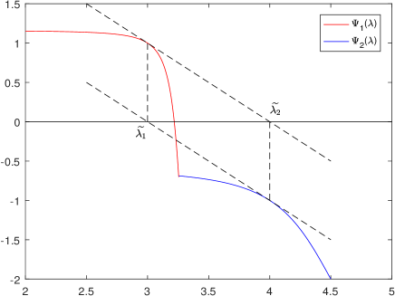
Figure 1: A counterexample for BNW

Now we modify the BNW procedure (refer to Algorithm 3 in Thom et al. (2015)) by adding a judging condition to get our modified BNW method (MBNW for short) as in Algorithm 7.

Algorithm 7 Modified bisection Newton (MBNW) method for finding the root of the equation $\Psi(\lambda)=0$

1:  set $i=0$, $\epsilon=1e-6$;

2:  if $\Psi(0)\leq 0$ then

3:     compute $\lambda^{*}$ using (12);

4:  else

5:     ${\rm lo}:=0$, ${\rm up}:=v_{{\rm 2nd-max}}$, $\lambda:={\rm lo}+\dfrac{1}{2}({\rm up}-{\rm lo})$;

6:     while not finished do

7:        update the bisection interval: if $\Psi(\lambda(i))>0$, then $\rm{lo}=\lambda(i)$; otherwise ${\rm up}=\lambda(i)$;

8:        $i=i+1$;

9:        if solver=Bisection then

10:           $\lambda(i):={\rm lo}+\dfrac{1}{2}({\rm up}-{\rm lo})$;

11:        else

12:           if solver=Newton then

13:              $\lambda(i):=\lambda(i-1)-\Psi(\lambda(i-1))/\Psi^{\prime}(\lambda(i-1))$;

14:           end if

15:           if $\lambda(i)<{\rm lo}$ or $\lambda(i)>{\rm up}$ or $\lvert\lambda(i)-\lambda(i-2)\rvert\leq\epsilon$ then

16:              $\lambda(i):={\rm lo}+\dfrac{1}{2}({\rm up}-{\rm lo})$;

17:           end if

18:        end if

19:     end while

20:     one has found the interval of $\lambda^{*}$, compute $\lambda^{*}$ using (12);

21:  end if

3 The gradient projection algorithm for SCoTLASS problems

3.1 The framework for GPSPCA

In this section, we bring forward the GP algorithm for SCoTLASS problems (SPCA-P1), (SPCA-P2) and (SPCA-P3) (GPSPCA for short) based on the projection method proposed in Liu et al. (2020), Barzilai-Borwein (BB) stepsize and the deflation method in the context of PCA.

There are mainly two methodologies utilized in PCA. The first is the greedy approach, that is, deflation method Mackey (2009), such as SCoTLASS Trendafilov and Jolliffe (2006), ConGradU Witten et al. (2009) Gpower${}_{\ell_{1}}$ Journée et al. (2010), etc. Deflation method in PCA is to find $r$ principal components by solving the optimization problem (1) sequentially one-by-one on the deflated data matrix or data covariance. Specifically, for a given data matrix $A\in{\mathbb{R}}^{m\times n}$ (without loss of generality, it is assumed that the variables contained in the columns of $A$ are centred), denoted by $\Sigma_{0}=A^{T}A\in{\mathbb{R}}^{n\times n}$ the sample covariance matrix. Then the sample covariance matrix $\Sigma_{j}$ ($j=1,2,\ldots,r$) should be updated recursively to eliminate the influence of the previous computed loading as follows Mackey (2009); Journée et al. (2010):

$$\Sigma_{j}=(I-{\bm{x}}_{j}{\bm{x}}_{j}^{T})\Sigma_{j-1}(I-{\bm{x}}_{j}{\bm{x}}_{j}^{T}).$$ (22)

The second is the block approach. Typical methods include SPCA Zou et al. (2006), Gpower${}_{\ell_{1},k}$ Journée et al. (2010), ALSPCA Lu and Zhang (2012) and BCD-SPCA Zhao et al. (2015); Yang (2017), GeoSPCA Bertsimas and Kitane (2022) etc. These methods aim to calculate multiple sparse PCs at once by utilizing certain block optimization techniques. However, we use the above described deflation method in this paper.

According to Algorithm 2, Algorithm 3 and Algorithm 4, which computes projections $P_{\Omega_{1}}({\bm{v}})$, $P_{\Omega_{2}}({\bm{v}})$ and $P_{\Omega_{3}}({\bm{v}})$ of a vector ${\bm{v}}\in{\mathbb{R}}^{n}$ onto $\Omega_{1}$, $\Omega_{2}$ and $\Omega_{3}$, respectively, the proposed GPSPCA algorithm is described informally in the following Algorithm 8 (denoted by GP-P1, GP-P2 or GP-P3 when the constraint set of SPCA problem is taken to be $\Omega_{1}$, $\Omega_{2}$ or $\Omega_{3}$, which corresponding SPCA-P1, SPCA-P2 or SPCA-P3 model of the SCoTLASS problem, respectively).

Algorithm 8 Gradient projection algorithm for SPCA, GPSPCA

1:  input data matrix $A\in R^{m\times n}$ and normalize, compute covariance matrix $\Sigma=A^{T}A$.

2:  initialize the count variable $i$, input the number of principal components $r$;

3:  while $i\leq r$ do

4:     find the index $j$ for the maximum value of diag($\Sigma$);

5:     given ${\bm{x}}^{0}=\theta$, set ${\bm{x}}^{(0)}_{j}=1$ and $\gamma_{0}>0$, initialize $k=0$;

6:     choose a small parameter $\gamma_{\min}>0$ and a large parameter $\gamma_{\max}>\gamma_{\min}$;

7:     while $\|{\rm P}_{\Omega}({\bm{x}}^{k}+\gamma_{k}{\bm{g}}^{k})-{\bm{x}}^{k}\|\neq 0$ do

8:        choose ${\bm{x}}^{k+1}\in{\rm P}_{\Omega}({\bm{x}}^{k}+\gamma_{k}{\bm{g}}^{k})$ (where $\Omega=\Omega_{1}$, $\Omega_{2}$ or $\Omega_{3}$, and using Algorithm 2, Algorithm 3 or Algorithm 4, respectively);

9:        set ${\bm{s}}^{k}={\bm{x}}^{k+1}-{\bm{x}}^{k}$, set ${\bm{y}}^{k}={\bm{g}}^{k+1}-{\bm{g}}^{k}$;

10:        compute $b_{k}=\langle{\bm{s}}^{k},{\bm{y}}^{k}\rangle$;

11:        if $b_{k}\leq 0$ then

12:           set $\gamma_{k+1}=\gamma_{\max}$;

13:        else

14:           compute $a_{k}=\langle{\bm{s}}^{k},{\bm{s}}^{k}\rangle$;

15:           set $\gamma_{k+1}=\min\{\gamma_{\max},\max\{\gamma_{\min},a_{k}/b_{k}\}\}$;

16:        end if

17:        set $k\leftarrow k+1$;

18:     end while

19:     find the $i$th component ${\bm{x}}^{k}$, set SPC$(i)={\bm{x}}^{k}$;

20:     update the data matrix $A=A-A*{\bm{x}}^{k}*({\bm{x}}^{k})^{T}$;

21:     compute the deflated covariance matrix $\Sigma=A^{T}A$;

22:     set $i\leftarrow i+1$;

23:  end while

Theorem 8

(The equivalence of GP-P1 and GP-P3) The solution to SCoTLASS problems (SPCA-P1) and (SPCA-P3) are the same by using GP-P1 and GP-P3, respectively.

Proof.  From (SPCA-P1) and (SPCA-P3), we know that the SCoTLASS problem is to maximize a convex function $f({\bm{x}})={\bm{x}}^{T}\Sigma{\bm{x}}$ with a semi-definite covariance matrix $\Sigma=A^{T}A$. However, the constraint sets $\Omega_{1}$ of SPCA-P1 problem and $\Omega_{3}$ of SPCA-P3 problem are both non-empty closed bounded sets contained in ri(dom($f$)) $={\mathbb{R}}^{n}$, and $\Omega_{1}$ is also convex. According to Corollary 32.3.2 in Rockafellar (1972), the maximum of $f$ on $\Omega_{1}$ exists and is obtained at some extreme point of $\Omega_{1}$. In the following, we will prove that the set of extreme points of $\Omega_{1}$ is exactly $\Omega_{3}$.

In fact, suppose ${\bm{x}}\in\Omega_{3}$. We are going to prove ${\bm{x}}$ is an extreme point of $\Omega_{1}$. Assume that ${\bm{x}}=(1-\mu){\bm{y}}+\mu{\bm{z}}$ for some $\mu\in(0,1)$ and ${\bm{y}},{\bm{z}}\in\Omega_{1}$, then $\|{\bm{y}}\|_{2}\leq 1$ and $\|{\bm{z}}\|_{2}\leq 1$. If $\|{\bm{y}}\|_{2}<1$ or $\|{\bm{z}}\|_{2}<1$, from the properties of norm we have

$$\|{\bm{x}}\|_{2}\leq(1-\mu)\|{\bm{y}}\|_{2}+\mu\|{\bm{z}}\|_{2}<(1-\mu)+\mu=1,$$

which is contradict with ${\bm{x}}\in\Omega_{3}$. So it must hold $\|{\bm{y}}\|_{2}=1$ and $\|{\bm{z}}\|_{2}=1$.

If ${\bm{y}}\neq{\bm{z}}$, by Cauchy-Schwartz inequality, we have

$$\begin{split}\|{\bm{x}}\|_{2}=&~{}[(1-\mu){\bm{y}}+\mu{\bm{z}}]^{T}[(1-\mu){\bm{y}}+\mu{\bm{z}}]\\ =&~{}(1-\mu)^{2}\|{\bm{y}}\|_{2}^{2}+2\mu(1-\mu){\bm{y}}^{T}{\bm{z}}+\mu^{2}\|{\bm{z}}\|_{2}^{2}\\ <&~{}(1-\mu)^{2}+2\mu(1-\mu)\|{\bm{y}}\|_{2}\|{\bm{z}}\|_{2}+\mu^{2}=1,\end{split}$$ (23)

which is again contradict with ${\bm{x}}\in\Omega_{3}$. Therefore, ${\bm{y}}={\bm{z}}$. Meanwhile, ${\bm{x}}=(1-\mu){\bm{y}}+\mu{\bm{z}}=(1-\mu){\bm{y}}+\mu{\bm{y}}={\bm{y}}={\bm{z}}$. To sum up, we know that ${\bm{x}}$ is an extreme point of $\Omega_{1}$.

However, suppose ${\bm{x}}\in\Omega_{1}\backslash\Omega_{3}$. If $\|{\bm{x}}\|_{2}<1,\|{\bm{x}}\|_{1}<t$, since ${\bm{x}}$ is an interior point of $\Omega_{1}$, it could not be an extreme point. In fact, there exists a $r>0$ such that the ball $B_{r}({\bm{x}})\subseteq\Omega_{1}$. Meanwhile let ${\bm{y}}$ and ${\bm{z}}$ are the two endpoints of a diameter of this ball. Then ${\bm{y}},{\bm{z}}\in\Omega_{1}$ (as $\Omega_{1}$ is a closed subset) and ${\bm{x}}=\frac{1}{2}{\bm{y}}+\frac{1}{2}{\bm{z}}$, which implies that ${\bm{x}}$ is not an extreme point of $\Omega_{1}$.

If $\|{\bm{x}}\|_{2}<1,\|{\bm{x}}\|_{1}=t$, let assume that ${\bm{x}}$ is in one of a hyperplane of ${\mathbb{S}}_{1}^{t}$. It easily follows that ${\bm{x}}$ is a relative interior point of the intersection set $C$ of this hyperplane and $\Omega_{1}$. Then from Theorem 6.4 in Rockafellar (1972) we know for all ${\bm{y}}\in C$, there exists a $\mu>1$ such that $(1-\mu){\bm{y}}+\mu{\bm{x}}\in C$. Take ${\bm{y}}\in\Omega_{2}\cap C\subseteq\Omega_{1}$ and the associated $\mu>1$, let ${\bm{z}}=(1-\mu){\bm{y}}+\mu{\bm{x}}\in C\subseteq\Omega_{1}$. Then we have ${\bm{x}}=\frac{1}{\mu}{\bm{z}}+\frac{\mu-1}{\mu}{\bm{y}}$, and $\frac{1}{\mu},\frac{\mu-1}{\mu}\in(0,1)$, $\frac{1}{\mu}+\frac{\mu-1}{\mu}=1$. That is, ${\bm{x}}$ is a convex combination of two different points ${\bm{y}},{\bm{z}}\in\Omega_{1}$, which implies that ${\bm{x}}$ is not an extreme point of $\Omega_{1}$.

Thus we have shown each point ${\bm{x}}\in\Omega_{1}\backslash\Omega_{3}$ is not an extreme point of $\Omega_{1}$. This completes the proof.

3.2 Convergence results

In this subsection, we will prove the global convergence of our proposed GPSPCA algorithm using the analysis in Bolte et al. (2014).

Bolte et al considered a broad class of nonconvex-nonsmooth problems in Bolte et al. (2014) of the form

$$\hbox{minimize}_{{\bm{x}},{\bm{y}}}\quad F({\bm{x}},{\bm{y}})=f({\bm{x}})+g({\bm{y}})+H({\bm{x}},{\bm{y}}),\quad({\bm{x}},{\bm{y}})\in{\mathbb{R}}^{n}\times{\mathbb{R}}^{m}$$ (M)

where $f:{\mathbb{R}}^{n}\rightarrow(-\infty,+\infty]$ and $g:{\mathbb{R}}^{m}\rightarrow(-\infty,+\infty]$ are both proper closed functions and $H:{\mathbb{R}}^{n}\times{\mathbb{R}}^{m}\rightarrow{\mathbb{R}}$ is a smooth function.

Starting with some given initial point $({\bm{x}}^{0},{\bm{y}}^{0})$, they generate an iterated sequence $\{({\bm{x}}^{k},{\bm{y}}^{k})\}_{k\in{\mathbb{N}}}$ in Bolte et al. (2014) via the proximal regularization for $H$ linearized at a given point of the Gauss-Seidel scheme :

$$\begin{split}&{\bm{x}}^{k+1}\in\hbox{arg}\min\limits_{{\bm{x}}\in{\mathbb{R}}^{n}}\{\langle{\bm{x}}-{\bm{x}}^{k},\nabla H_{\bm{x}}({\bm{x}}^{k},{\bm{y}}^{k})\rangle+\dfrac{c_{k}}{2}\|{\bm{x}}-{\bm{x}}^{k}\|_{2}^{2}+f({\bm{x}}^{k})\}\\ &{\bm{y}}^{k+1}\in\hbox{arg}\min\limits_{{\bm{y}}\in{\mathbb{R}}^{m}}\{\langle{\bm{y}}-{\bm{y}}^{k},\nabla H_{{\bm{y}}}({\bm{x}}^{k+1},{\bm{y}}^{k})\rangle+\dfrac{d_{k}}{2}\|{\bm{y}}-{\bm{y}}^{k}\|_{2}^{2}+g({\bm{y}}^{k})\}\end{split}$$ (24)

where $c_{k}$ and $d_{k}$ are positive real numbers, and yield the Proximal Alternating Linearized Minimization (PALM for short) algorithm.

Remark 9

PALM reduces to Proximal Forward-Backward (PFB) algorithm when there is no ${\bm{y}}$ term. In this case, $F({\bm{x}}):=f({\bm{x}})+h({\bm{x}})$ (where $h({\bm{x}})\equiv H({\bm{x}},\bf{0})$), and the proximal forward-backward scheme for minimizing $\Psi$ can simply be viewed as the proximal regularization of $h$ linearized at a given point ${\bm{x}}^{k}$, i.e.,

$${\bm{x}}^{k+1}\in{\rm arg}\min\limits_{{\bm{x}}\in{\mathbb{R}}^{n}}\{\langle{\bm{x}}-{\bm{x}}^{k},\nabla h({\bm{x}}^{k})\rangle+\dfrac{t_{k}}{2}\|{\bm{x}}-{\bm{x}}^{k}\|_{2}^{2}+f({\bm{x}}^{k})\}$$ (25)

It is well-known that PFB reduces to the gradient projection (GP) method when $f=\delta_{\Omega}$ (where $\Omega$ is a nonempty, closed and nonconvex subset of ${\mathbb{R}}^{n}$, i.e., GP method generates an iterated sequence $\{{\bm{x}}^{k}\}_{k\in{\mathbb{N}}}$ via

$${\bm{x}}^{k+1}\in P_{\Omega}({\bm{x}}^{k}-\dfrac{1}{t_{k}}\nabla h({\bm{x}}^{k}))$$ (26)

To describe the global convergence of PFB, let us first give the definition of Kurdyka-Łojasiewicz (KL) function Bolte et al. (2014). Let $\eta\in(0,+\infty]$. We denote by $\Phi_{\eta}$ the class of all concave and continuous functions $\varphi:[0,\eta)\rightarrow{\mathbb{R}}^{+}$ which satisfy the following conditions

(i) $\varphi(0)=0$;

(ii) $\varphi$ is smooth on $(0,\eta)$ and continuous at 0;

(iii) for all $s\in(0,\eta)$, $\varphi^{\prime}(s)>0$.

Definition (Kurdyka-Łojasiewicz property, Definition 3 in Bolte et al. (2014)) Let $\sigma:{\mathbb{R}}^{d}\rightarrow(-\infty,+\infty]$ be proper and lower semi-continuous.

(i) The function $\sigma$ is said to have the Kurdyka-Łojasiewicz (KL) property at $\bar{u}\in\hbox{dom}\partial\sigma:=\{u\in{\mathbb{R}}^{d}:\partial\sigma(u)\neq\emptyset\}$, if there exist $\eta\in(0,+\infty]$, a neighborhood $U$ of $\bar{u}$ and a function $\varphi\in\Phi_{\eta}$, such that for all

$$u\in U\cap\{u\in{\mathbb{R}}^{d}:\sigma(\bar{u})<\sigma(u)<\sigma(\bar{u})+\eta\},$$

the following inequality holds

$$\varphi^{\prime}(\sigma(u)-\sigma(\bar{u}))\cdot\hbox{dist}(0,\partial\sigma(u))\geq 1.$$

(ii) If $\sigma$ satisfy the KL property at each point of domain $\partial\sigma$, then $\sigma$ is called a KL function.

With some assumptions, Bolte et al proved the global convergence for PALM algorithm, and consequently the global convergence for PFB algorithm in Bolte et al. (2014).

Proposition 10

(Proposition 3 in Bolte et al. (2014)) (A convergence result of PFB) Let $h:{\mathbb{R}}^{n}\rightarrow{\mathbb{R}}$ be a continuously differentiable function with gradient $\nabla h$ assumed $L_{h}$-Lipschitz continuous and let $f:{\mathbb{R}}^{n}\rightarrow(-\infty,+\infty]$ be a proper and lower semi-continuous function with $\inf\limits_{{\mathbb{R}}^{n}}f>-\infty$. Assume that $F=f+h$ is a KL function. Let $\{{\bm{x}}^{k}\}_{k\in{\mathbb{N}}}$ be a sequence generated by PFB which is assumed to be bounded and let $t_{k}>L_{h}$. The following assertions hold:

(i) The sequence $\{{\bm{x}}^{k}\}_{k\in{\mathbb{N}}}$ has finite length, that is,

$$\sum\limits_{k=1}^{\infty}\|{\bm{x}}^{k+1}-{\bm{x}}^{k}\|_{2}<+\infty.$$ (27)

(ii) The sequence $\{{\bm{x}}^{k}\}_{k\in{\mathbb{N}}}$ converges to a critical point ${\bm{x}}^{*}$ of $F$.

Consider the SCoTLASS problems (SPCA-P1), (SPCA-P2) and (SPCA-P3), they can be reformulated respectively as

$$\begin{array}[]{rc}{\rm minimize}&-{\bm{x}}^{T}\Sigma{\bm{x}}\\ {\rm s.t.}&{\bm{x}}\in\Omega_{i}\end{array},~{}~{}i=1,2,3$$ (28)

In Proposition 10, taking $h({\bm{x}})=-{\bm{x}}^{T}\Sigma{\bm{x}}$,

$$f_{i}({\bm{x}})=\delta_{\Omega_{i}}({\bm{x}})=\begin{cases}0,&{\bm{x}}\in\Omega_{i}\\ +\infty,&{\bm{x}}\notin\Omega_{i}\end{cases},~{}~{}i=1,2,3$$

which is the indicator function on $\Omega_{i}$, and $F_{i}({\bm{x}})=h({\bm{x}})+f_{i}({\bm{x}})=-{\bm{x}}^{T}\Sigma{\bm{x}}+\delta_{\Omega_{i}}({\bm{x}})$, $i=1,2,3$. Then, we can obtain the global convergence for our GPSPCA algorithm on different constraint sets $\Omega_{1}$, $\Omega_{2}$ and $\Omega_{3}$.

In fact, $\Sigma=A^{T}A$ is positive semidefinite, $\nabla h=-2\Sigma{\bm{x}}$. By the Cauchy-Schwartz inequality, we have for all ${\bm{x}},{\bm{y}}\in{\mathbb{R}}^{n}$,

$$\|\nabla h({\bm{x}})-\nabla h({\bm{y}})\|_{2}=2\|\Sigma({\bm{x}}-{\bm{y}})\|_{2}\leq 2\|\Sigma\|_{2}\|{\bm{x}}-{\bm{y}}\|_{2}=2\lambda_{\max}(\Sigma)\|{\bm{x}}-{\bm{y}}\|_{2}.$$

That is, $h$ is Lipschitz continuous with moduli $L_{h}=2\lambda_{\max}(\Sigma)$ (here $\lambda_{\max}(\Sigma)$ denotes the largest eigenvalue of $\Sigma$). Since $\Omega_{i},i=1,2,3$ are all nonempty compact closed sets, it easily follows that $f_{i}({\bm{x}})=\delta_{\Omega_{i}}({\bm{x}}),i=1,2,3$ are all proper and lower semi-continuous. And

$$\inf\limits_{{\mathbb{R}}^{n}}f({\bm{x}})=\inf\limits_{{\mathbb{R}}^{n}}\delta_{\Omega_{i}}({\bm{x}})=0>-\infty.$$

Now we show that $F_{i}({\bm{x}}),i=1,2,3$ are all KL functions.

According to the properties of semi-algebraic functions Bolte et al. (2014), we know that a semi-algebraic function must be a KL function, and the finite sum of semi-algebraic functions is also semi-algebraic. And $h({\bm{x}})=-{\bm{x}}^{T}\Sigma{\bm{x}}$ is actually a polynomial function, from Appendix Example 2 in Bolte et al. (2014), we have that $h({\bm{x}})$ is a semi-algebraic function. Thus the only thing is to show that $\delta_{\Omega_{i}}({\bm{x}}),i=1,2,3$ are semi-algebraic functions. However, the indicator function of a semi-algebraic set must be a semi-algebraic function. Remaining we prove $\Omega_{i},i=1,2,3$ are all semi-algebraic sets.

From the definition of the semi-algebraic set, for $S\subset{\mathbb{R}}^{d}$, if there exists a finite number of real polynomial functions $g_{ij},h_{ij}:{\mathbb{R}}^{d}\rightarrow{\mathbb{R}}$ such that

$$S=\mathop{\bigcup}\limits_{j=1}^{p}\mathop{\bigcap}\limits_{i=1}^{q}\left\{{\bm{u}}\in{\mathbb{R}}^{d}:g_{ij}({\bm{u}})=0,h_{ij}({\bm{u}})<0\right\}$$ (29)

then $S$ is a semi-algebraic set. Notice that

$$\{{\bm{x}}\in{\mathbb{R}}^{n}:\sum\limits_{k=1}^{n}\lvert x_{k}\rvert-t=0\}=\bigcup\limits_{i=1}^{2^{n}}\{{\bm{x}}\in{\mathbb{R}}^{n}:{\bm{e}}_{i}^{T}{\bm{x}}-t=0\}$$ (30)

and

$$\{{\bm{x}}\in{\mathbb{R}}^{n}:\sum\limits_{k=1}^{n}\lvert x_{k}\rvert-t<0\}=\bigcap\limits_{i=1}^{2^{n}}\{{\bm{x}}\in{\mathbb{R}}^{n}:{\bm{e}}_{i}^{T}{\bm{x}}-t<0\}$$ (31)

where the $j$-th ($j=1,\ldots,n$) component ${\bm{e}}_{ij}$ of ${\bm{e}}_{i}$ takes value in $\{-1,1\}$. We have $\{{\bm{x}}\in{\mathbb{R}}^{n}:\sum\limits_{k=1}^{n}\rvert x_{k}\rvert-t=0\}$ and $\{{\bm{x}}\in{\mathbb{R}}^{n}:\sum\limits_{k=1}^{n}\lvert x_{k}\rvert-t<0\}$ are semi-algebraic sets. And

$$\{{\bm{x}}\in{\mathbb{R}}^{n}:\sum\limits_{k=1}^{n}x_{k}^{2}-1=0\},~{}~{}\{{\bm{x}}\in{\mathbb{R}}^{n}:\sum\limits_{k=1}^{n}x_{k}^{2}-1<0\}$$ (32)

are clearly semi-algebraic sets. Therefore $\Omega_{i},i=1,2,3$ are all semi-algebraic sets.

By Proposition 10 and Remark 9, we have the following global convergence result of our GPSPCA algorithm for SCoTLASS problems (SPCA-P1), (SPCA-P2) and (SPCA-P3).

Theorem 11

(Global convergence of GPSPCA) Let $\{{\bm{x}}^{k}\}_{k\in{\mathbb{N}}}$ be a sequence generated by GPSPCA which is assumed to be bounded and let $t_{k}>2\lambda_{\max}(\Sigma)$. The following assertions hold:

(i) The sequence $\{{\bm{x}}^{k}\}_{k\in{\mathbb{N}}}$ has finite length, that is, (27) holds;

(ii) The sequence $\{{\bm{x}}^{k}\}_{k\in{\mathbb{N}}}$ converges to a critical point ${\bm{x}}^{*}$ of $F({\bm{x}})=-{\bm{x}}^{T}\Sigma{\bm{x}}+\delta_{\Omega}({\bm{x}})$, i.e. ${\bm{x}}^{*}$ satisfies $0\in\partial F$, $\Omega=\Omega_{1}$, $\Omega_{2}$ or $\Omega_{3}$.

4 The approximate Newton algorithm for SCoTLASS problems

In Hager et al. (2016), besides the GP algorithm, Hager et al. also proposed an approximate Newton algorithm for non-convex minimization and applied it to SPCA. They pointed out that in some cases, the approximate Newton algorithm with a Barzilai-Borwein (BB) Hessian approximation and a non-monotone line search can be substantially faster than the other algorithms, and can converge to a better solution.

For $f:{\mathbb{R}}^{n}\rightarrow{\mathbb{R}}$ a concave second-order continuously differentiable function, and $\Omega$ a compact nonempty set, they consider the algorithm in which the new iterate ${\bm{x}}_{k+1}$ is obtained by optimizing the quadratic model:

$${\bm{x}}_{k+1}\in{\rm arg}\min\{\nabla f({\bm{x}}_{k})({\bm{x}}-{\bm{x}}_{k})+\frac{\alpha_{k}}{2}\|{\bm{x}}-{\bm{x}}_{k}\|_{2}^{2}:{\bm{x}}\in\Omega\}.$$ (33)

Notice that after completing the square, the iteration is equivalent to

$${\bm{x}}_{k+1}\in{\rm arg}\min\{\alpha_{k}\|{\bm{x}}-({\bm{x}}_{k}-g_{k}/\alpha_{k})\|_{2}^{2}:{\bm{x}}\in\Omega\},$$ (34)

where $g_{k}=\nabla f({\bm{x}}_{k})$. If $\alpha_{k}>0$, then this reduces to ${\bm{x}}_{k+1}\in{\rm P}_{\Omega}({\bm{x}}_{k}-g_{k}/\alpha_{k})$; in other words, perform the gradient projection algorithm with step size $1/\alpha_{k}$. If $\alpha_{k}<0$, then the iteration reduces to

$${\bm{x}}_{k+1}\in{\rm Q}_{\Omega}({\bm{x}}_{k}-g_{k}/\alpha_{k}),$$ (35)

where

$${\rm Q}_{\Omega}({\bm{x}})={\rm arg}\max\{\|{\bm{x}}-{\bm{y}}\|_{2}^{2}:{\bm{y}}\in\Omega\}.$$ (36)

To design the approximate Newton algorithm for SCoTLASS problems, let us first characterize the solutions to the problems ${\rm Q}_{\Omega_{1}}({\bm{x}})$, ${\rm Q}_{\Omega_{2}}({\bm{x}})$ and ${\rm Q}_{\Omega_{3}}({\bm{x}})$.

Proposition 12

For $\forall{\bm{x}}\in{\mathbb{R}}^{n}$, the solution to the problems ${\rm Q}_{\Omega_{1}}({\bm{x}})$ and ${\rm Q}_{\Omega_{3}}({\bm{x}})$ are the same.

Proof.   $\forall{\bm{x}}\in{\mathbb{R}}^{n}$, the problems ${\rm Q}_{\Omega_{1}}({\bm{x}})$ and ${\rm Q}_{\Omega_{3}}({\bm{x}})$ are both to maximize a convex function $f({\bm{y}})=\|{\bm{x}}-{\bm{y}}\|_{2}^{2}$. Then the rest of the proof is the same as that in Theorem 8.

Proposition 13

For $\forall{\bm{x}}\in{\mathbb{R}}^{n}$, we have

$${\rm arg}\max\limits_{{\bm{y}}\in\Omega_{2}}\|{\bm{x}}-{\bm{y}}\|_{2}^{2}=-{\rm arg}\min\limits_{{\bm{y}}\in\Omega_{2}}\|{\bm{x}}-{\bm{y}}\|_{2}^{2},$$ (37)

$${\rm arg}\max\limits_{{\bm{y}}\in\Omega_{3}}\|{\bm{x}}-{\bm{y}}\|_{2}^{2}=-{\rm arg}\min\limits_{{\bm{y}}\in\Omega_{3}}\|{\bm{x}}-{\bm{y}}\|_{2}^{2}.$$ (38)

That is,

$${\rm Q}_{\Omega_{i}}({\bm{x}})=-{\rm P}_{\Omega_{i}}({\bm{x}}),~{}~{}i=2,3.$$ (39)

Proof.

$$\begin{array}[]{rl}&{\rm arg}\max\limits_{{\bm{y}}\in\Omega_{2}}\|{\bm{x}}-{\bm{y}}\|_{2}^{2}\\ =&{\rm arg}\max\limits_{{\bm{y}}\in\Omega_{2}}\{\|{\bm{x}}\|_{2}^{2}-2\langle{\bm{x}},{\bm{y}}\rangle+\|{\bm{y}}\|_{2}^{2}\}\\ =&{\rm arg}\max\limits_{{\bm{y}}\in\Omega_{2}}\{\|{\bm{x}}\|_{2}^{2}-2\langle{\bm{x}},{\bm{y}}\rangle+1\}~{}~{}(\hbox{since }{\bm{y}}\in\Omega_{2},\|{\bm{y}}\|_{2}=1)\\ =&{\rm arg}\max\limits_{{\bm{y}}\in\Omega_{2}}-2\langle{\bm{x}},{\bm{y}}\rangle={\rm arg}\max\limits_{{\bm{y}}\in\Omega_{2}}2\langle{\bm{x}},-{\bm{y}}\rangle~{}~{}(\hbox{since }\|{\bm{x}}\|_{2}\hbox{ is a constant})\\ =&{\rm arg}\min\limits_{{\bm{y}}\in\Omega_{2}}-2\langle{\bm{x}},-{\bm{y}}\rangle={\rm arg}\min\limits_{{\bm{y}}\in\Omega_{2}}\|{\bm{x}}-(-{\bm{y}})\|_{2}^{2}\\ =&{\rm arg}\min\limits_{-{\bm{y}}\in\Omega_{2}}\|{\bm{x}}-{\bm{y}}\|_{2}^{2}=-{\rm arg}\min\limits_{{\bm{y}}\in\Omega_{2}}\|{\bm{x}}-{\bm{y}}\|_{2}^{2}.~{}~{}(\hbox{since }\Omega_{2}\hbox{ is symmetrical about the origin})\end{array}$$

The proof for $\Omega_{3}$ is similar.

Now we can design the approximate Newton algorithms for SCoTLASS problems (SPCA-P1), (SPCA-P2) and (SPCA-P3) (ANSPCA for short) based on the projection method proposed in Liu et al. (2020) and Barzilai-Borwein (BB) stepsize and the deflation method in the context of PCA in the following Algorithm 9 (denoted by AN-P1, AN-P2 and AN-P3, respectively, when the constraint set of SPCA is taken to be $\Omega_{1}$, $\Omega_{2}$ or $\Omega_{3}$, which corresponding SPCA-P1, SPCA-P2 or SPCA-P3 model of the SCoTLASS problem, respectively).

From Proposition 12, ${\rm Q}_{\Omega_{1}}({\bm{x}})$ and ${\rm Q}_{\Omega_{3}}({\bm{x}})$ have the same solutions, and from Proposition 13, the optimal solutions of ${\rm Q}_{\Omega_{2}}({\bm{x}})$ and ${\rm Q}_{\Omega_{3}}({\bm{x}})$ can be obtained by the projections ${\bm{x}}$ onto $\Omega_{2}$ and $\Omega_{3}$, respectively. So we take the the optimal solution ${\rm Q}_{\Omega_{3}}({\bm{x}})$ as the the optimal solution ${\rm Q}_{\Omega_{1}}({\bm{x}})$ in Algorithm 9.

Algorithm 9 Approximate Newton algorithm for SPCA, ANSPCA

1:  input data matrix $A\in{\mathbb{R}}^{m\times n}$ and normalize, compute covariance matrix $\Sigma$.

2:  initialize the count variable $i$, input the number of principal components $r$;

3:  while $i\leq r$ do

4:     take $\sigma\in(0,1)$, $\left[\alpha_{\min},\alpha_{\max}\right]\subset(-\infty,0)$;

5:     find the index $j$ for the maximum value of diag($\Sigma$), given ${\bm{x}}^{0}={\bm{e}}$, set ${\bm{x}}^{1}_{j}=1$ and $\gamma_{0}\geq 0$, compute ${\bm{x}}^{2}=P_{\Omega}({\bm{x}}^{1}+g^{1})$;

6:     initialize $k=1$;

7:     while $\|{\bm{P}}_{\Omega}({\bm{x}}^{k}+\gamma_{k}{\bm{g}}^{k})-{\bm{x}}^{k}\|\neq 0$ do

8:        set ${\bm{s}}^{k}={\bm{x}}^{k+1}-{\bm{x}}^{k}$, ${\bm{y}}^{k}={\bm{g}}^{k+1}-{\bm{g}}^{k}$;

9:        compute $b_{k}=\langle{\bm{s}}^{k},{\bm{y}}^{k}\rangle$, $a_{k}=\langle{\bm{s}}^{k},{\bm{s}}^{k}\rangle$, $\alpha_{k}^{BB}=\dfrac{b_{k}}{a_{k}}$;

10:        compute $\beta_{k}={\rm mid}(\alpha_{\min},\alpha_{k}^{{\rm BB}},\alpha_{\max})$, set $j_{k}=0$, initialize $\alpha_{k}=\sigma^{j_{k}}\beta_{k}$;

11:        take $f_{k+1}^{\max}=\max\left\{f({\bm{x}}^{k+1-j}):0\leq j\leq\min\left\{k+1,M\right\}\right\}$, and choose ${\bm{x}}^{k+2}\in-P_{\Omega}({\bm{x}}^{k+1}-{\bm{g}}^{k}/\alpha_{k})$ (where $\Omega=\Omega_{1}$, $\Omega_{2}$ or $\Omega_{3}$, and using Algorithm 4, Algorithm 3 or Algorithm 4, respectively);

12:        while $f_{k+2}>f_{k+1}^{\max}+\dfrac{\alpha_{k}}{2}\|{\bm{x}}^{k+2}-{\bm{x}}^{k+1}\|^{2}$ do

13:           set $j_{k}=j_{k}+1$, $\alpha_{k}=\sigma^{j_{k}}\beta_{k}$, and choose ${\bm{x}}^{k+2}\in-P_{\Omega}({\bm{x}}^{k+1}-{\bm{g}}_{k}/\alpha_{k})$ (where $\Omega=\Omega_{1}$, $\Omega_{2}$ or $\Omega_{3}$, and using Algorithm 4, Algorithm 3 or Algorithm 4, respectively);

14:        end while

15:        set $k\leftarrow k+1$;

16:     end while

17:     find the $i$th component ${\bm{x}}^{k}$, set SPC$(i)={\bm{x}}^{k}$;

18:     update the data matrix $A=A-A*{\bm{x}}^{k}*({\bm{x}}^{k})^{T}$;

19:     compute the deflated covariance matrix $\Sigma=A^{T}A$;

20:     set $i\leftarrow i+1$;

21:  end while

By Theorem 3.4 and Theorem 3.5 in Hager et al. (2016), we also have the following convergence result of our ANSPCA algorithm for SCoTLASS problems (SPCA-P1), (SPCA-P2) and (SPCA-P3).

Theorem 14

(Global convergence of ANSPCA) Suppose that the covariance matrix $\Sigma=A^{T}A$ of data matrix $A$ satisfy that there exists a $\mu<0$ such that $2\Sigma+\mu I$ is positive semidefinite, and let $\{{\bm{x}}^{k}\}_{k\in{\mathbb{N}}}$ be a sequence generated by ANSPCA. Then the following assertions hold:

(i) the sequence of objective values $f({\bm{x}}_{k})$ generated by ANSPCA algorithm for memory $M>0$ converge to a limit $f^{*}$ as $k$ tends to infinity. If ${\bm{x}}^{*}$ is any limit point of the iterates ${\bm{x}}^{k}$, then ${\bm{x}}^{*}\in Q_{\Omega}({\bm{x}}^{*}-{\bm{g}}({\bm{x}}^{*})/\alpha)$ for some $\alpha<0$, and

$$\nabla f({\bm{x}}^{*})({\bm{y}}-{\bm{x}}^{*})\leq 0,\qquad{\forall}{\bm{y}}\in{\rm conv}(\Omega)$$ (40)

(ii) there exists a constant $c$ independent of $k$, such that

$$\min\{\|{\bm{x}}^{j+1}-{\bm{x}}^{j}\|_{2}:0<j<kM\}\leq\dfrac{c}{\sqrt{k}}.$$ (41)

Proof.  Theorem 3.4 and Theorem 3.5 in Hager et al. (2016) require two conditions:

(1) the objective function $f$ is continuously differentiable on a compact set $\Omega\subseteq{\mathbb{R}}^{n}$;

(2) the following inequality (42) holds for some $\mu<0$,

$$f({\bm{y}})\leq f({\bm{x}})+\nabla f({\bm{x}})^{T}({\bm{y}}-{\bm{x}})+\dfrac{\mu}{2}\|{\bm{y}}-{\bm{x}}\|^{2}$$ (42)

For SPCA problem with data matrix $A$ and covariance matrix $\Sigma=A^{T}A$, the objective function $f({\bm{x}})=-{\bm{x}}^{T}\Sigma{\bm{x}}$ is clearly continuously differentiable on the compact sets $\Omega_{1}$, $\Omega_{2}$ and $\Omega_{3}$. And if there exists a $\mu<0$ such that $2\Sigma+\mu I$ is positive semidefinite, then ${\bm{x}}^{T}(\Sigma+\dfrac{\mu}{2}){\bm{x}}=-f({\bm{x}})-\dfrac{-\mu}{2}\|{\bm{x}}\|^{2}$ is a convex function, which implies that $-f({\bm{x}})$ is a strongly convex function with module $-\mu$, and then

$$-f({\bm{y}})\geq-f({\bm{x}})-\nabla f({\bm{x}})^{T}({\bm{y}}-{\bm{x}})-\dfrac{\mu}{2}\|{\bm{y}}-{\bm{x}}\|^{2}.$$

By taking the opposite value in the two sides of the above inequality, one easily gets (42). Thus (i) and (ii) holds by Theorem 3.4 and Theorem 3.5 in Hager et al. (2016).

In fact, by the proof of Theorem 3.5 in Hager et al. (2016) we know the constant $c$ can be computed by $c=\sqrt{\dfrac{2(f({\bm{x}}_{0})-f^{*})}{\lvert\overline{\alpha}\rvert}}$, where $\overline{\alpha}=\max(\sigma\mu/2,\alpha_{\max})$.

5 Numerical experiments

In this section, we conduct several numerical experiments using MATLAB 2019 on a laptop with 8GB of RAM and an 1.80GHz Intel Core i7-8550U processor under WINDOWS 10, and present the experiment results which we have done to investigate the performance of our proposed GPSPCA and ANSPCA algorithms. On one hand, we contrast the similarities and differences of GPSPCA and ANSPCA among three projection subproblems on $\Omega_{1}={\mathbb{B}}_{1}^{t}\cap{\mathbb{B}}_{2}$, $\Omega_{2}={\mathbb{S}}_{1}^{t}\cap{\mathbb{S}}_{2}$ or $\Omega_{3}={\mathbb{B}}_{1}^{t}\cap{\mathbb{S}}_{2}$. On the other hand, we also compare the performance of our GPSPCA and ANSPCA algorithms with several typical SPCA algorithms: the $\ell_{1}$-constrained block coordinate descent approach (BCD-SPCA${}_{\ell_{1}}$) in Zhao et al. (2015) (which use and the $\ell_{0}$-constrained approximate Newton algorithm (GPBB) in Hager et al. (2016), the conditional gradient algorithm with unit step-size (ConGradU) proposed in Witten et al. (2009), the generalized $\ell_{1}$-penalized power method (Gpower${}_{\ell_{1}}$) in Journée et al. (2010).

In our experiments, when many principal components (PCs) are extracted, ConGrad and BCD-SPCA algorithms compute PC loadings on the Stiefel manifold simultaneously, while other algorithms all compute PC loadings successively using the deflation method. There are different ways to select the initialized vectors. In Hager et al. (2016), ${\bm{x}}^{0}=e_{i}$, the $i$-th column of the identity matrix, where $i$ is the index of the largest diagonal element of the covariance matrix $\Sigma$. In Journée et al. (2010), ${\bm{x}}^{0}$ is chosen parallel to the column of $A$ with the largest norm, that is,

$${\bm{x}}^{0}=\dfrac{a_{i^{*}}}{\|a_{i^{*}}\|_{2}},\;{\rm where}~{}i^{*}=\arg\max_{i}\|a_{i}\|_{2}.$$ (43)

In this paper, we mainly use the first initialization method.

In addition, in terms of sparse or penalty parameter selection, based on the given $\ell_{0}$ sparse parameter $k$ in the GPBB algorithm, the $\ell_{1}$ penalized parameter $\gamma$ of Gpower${}_{\ell_{1}}$ or $s$ of ConGradU are obtained carefully by grid search to achieve the desired sparsity, notice from Journée et al. (2010) that $\gamma\in[0,\|a_{i^{*}}\|_{2})$. And for the BCD-SPCA approach and the proposed GPSPCA and ANSPCA algorithms we easily select the appropriate $t$ according to the inequality $\|{\bm{x}}\|_{1}\leq\sqrt{\|{\bm{x}}_{0}\|}\|{\bm{x}}\|_{2}$.

5.1 Performance indexes

Refer to Trendafilov and Jolliffe (2006); Zou et al. (2006); Witten et al. (2009); Journée et al. (2010); Zhao et al. (2015); Hager et al. (2016), we use the following performance indexes:

Sparsity (or Cardinality):  Sparsity stands for the percentage of nonzero elements in the loading matrix. The smaller the sparsity is, the sparser the data is. And cardinality means the number of nonzero elements.

Non-orthogonality (non-ortho for short):  Let ${\bm{x}}_{i}$ and ${\bm{x}}_{j}$ be any two loading vectors, and the included angle between them is denoted by $\alpha_{ij}$. The non-orthogonality is defined by the maximum of $|90-\alpha_{ij}|$ over $i$ and $j$. The smaller this value is, the better the non-orthogonality is.

Correlation:  Represents for the maximum of the absolute value of correlation coefficients over all PCs.

Percentage of explained variance (PEV for short):  Means that the ratio of the tuned variance sum of the top $k$ sparse PCs to the variance sum of all PCs, it can be calculated as

$$\hat{Z}=QR$$ (44)

$$PEV=\sum_{j=1}^{n}R_{jj}^{2}$$ (45)

where $\hat{Z}$ is the modified sparse PC, and performed QR decomposition with $Q$ a orthogonal matrix and $R$ a upper triangular matrix.

Reconstruction error minimization criterion (RRE for short): RRE is defined as

$$RRE=\frac{\|A-\hat{A}\|_{F}}{\|A\|_{F}}$$ (46)

where $A$ denotes the data matrix, $\hat{A}=\hat{U}V^{T}$, $V$ is the loading matrix, $\hat{U}=AV(V^{T}V)^{-1}$.

Time:  The running time of the procedure.

Iterations:  The number of iterations computing the projection subproblem.

5.2 Termination Criterion

Denote by $f_{k}$ the value of the objective function for the $k$th iteration, $g_{k}$ the gradient for $k$th iteration, and $\varepsilon$ the tolerated error. Our GPSPCA and ANSPCA algorithms use the following stopping criterion:

1. Absolute error of the argument: $\|{\bm{x}}_{k}-{\bm{x}}_{k-1}\|_{2}<\varepsilon$;

2. Relative error of the objective function: $\|f_{k}-f_{k-1}\|_{\infty}<\varepsilon(1+\|f_{k-1}\|_{\infty})$;

3. Relative error of the gradient: $\|g_{k}-g_{k-1}\|_{\infty}<\varepsilon(1+\|g_{k-1}\|_{\infty})$;

4. Relative error of the argument: $\|{\bm{x}}_{k}-{\bm{x}}_{k-1}\|_{\infty}<\varepsilon\|{\bm{x}}_{k-1}\|_{\infty}$.

5.3 Simulations

In this subsection, we employ two artificially synthesized datasets to evaluate the performance of the proposed GPSPCA and ANSPCA algorithms, one is for recovering the ground truth sparse principal components underlying data, the other is for comparing the average computational time.

5.3.1 Hastie dataset

Hastie dataset was first introduced by Zou et al. Zou et al. (2006) to illustrate the advantage of sparse PCA over conventional PCA on sparse PC extraction. So far this dataset has become one of the most commonly utilized data for testing the effectiveness of sparse PCA methods. The dataset was generated in the following way: at first, three hidden variables $V_{1}$, $V_{2}$ and $V_{3}$ were defined as:

$$V_{1}\sim N(0,290)$$ (47)

$$V_{2}\sim N(0,300)$$ (48)

$$V_{3}=-0.3V_{1}+0.925V_{2}+\varepsilon$$ (49)

where $\varepsilon\sim N(0,1)$, $V_{1}$, $V_{2}$ and $\varepsilon$ are independent to each other. Then ten observation variables are generated by $V_{1}$, $V_{2}$ and $V_{3}$ as follows:

$$X_{i}=V_{1}+\varepsilon_{i}^{1},i=1,2,3,4$$ (50)

$$X_{i}=V_{2}+\varepsilon_{i}^{2},i=5,6,7,8$$ (51)

$$X_{i}=V_{3}+\varepsilon_{i}^{3},i=9,10$$ (52)

where $\varepsilon_{i}^{j}\sim N(0,1)$ and $\varepsilon_{i}^{j}$ ($j=1,2,3$, $i=1,...,10$) are independent to each other. Thus, only two principal components (PC) can include most information in the raw data. The first PC corresponding to $V_{1}$ can be computed by $X_{1}$, $X_{2}$, $X_{3}$, and $X_{4}$; the second PC corresponding to $V_{2}$ can be computed by $X_{5}$, $X_{6}$, $X_{7}$, and $X_{8}$.

In these experiments, the $\ell_{1}$ sparsity parameter $t$ in GPSPCA and ANSPCA are set to be $t=2$, taking $\sigma=0.25$, $M=50$ in ANSPCA.

Table 1: The simulation results of GPSPCA for Hastie data

	GP-P1		GP-P2		GP-P3
loading matrix	0	0.500774	0	0.500764	0	0.500774
	0	0.499742	0	0.499745	0	0.499742
	0	0.499742	0	0.499745	0	0.499742
	0	0.499742	0	0.499745	0	0.499742
	0.500119	0	0.500119	0	0.500119	0
	0.49996	0	0.49996	0	0.49996	0
	0.49996	0	0.49996	0	0.49996	0
	0.49996	0	0.49996	0	0.49996	0
	0	0	0	0	0	0
	0	0	0	0	0	0
sparsity	0.4		0.4		0.4
non-ortho	0		0		0
correlation	0		0		0
PEV(%)	80.4612163		80.4612168		80.4612163
RRE	0.442026964		0.442026958		0.442026964
time(s)	0.0218682		0.0124865		0.0186422
iterations	[4 3]		[4 3]		[4 3]

Table 2: The simulation results of ANSPCA for Hastie data

	AN-P1		AN-P2		AN-P3
loading matrix	0	0.500000	0	0.500000	0	0.500000
	0	0.499999	0	0.499999	0	0.499999
	0	0.499999	0	0.499999	0	0.499999
	0	0.499999	0	0.499999	0	0.499999
	0.500000	0	0.500000	0	0.500000	0
	0.499999	0	0.499999	0	0.499999	0
	0.499999	0	0.499999	0	0.499999	0
	0.499999	0	0.499999	0	0.499999	0
	0	0	0	0	0	0
	0	0	0	0	0	0
sparsity	0.4		0.4		0.4
non-ortho	0		0		0
correlation	0		0		0
PEV(%)	80.461238		80.461238		80.461238
RRE	0.442027		0.442027		0.442027
time(s)	0.0138333		0.0121649		0.010145
iterations	[6 4]		[6 4]		[6 4]

Table 1 and Table 2 present the values of the above performance indexes for GPSPCA, ANSPCA. From the Table 1 and Table 2 we see that for SCoTLASS problems (SPCA-P1), (SPCA-P2) and (SPCA-P3), GPSPCA and ANSPCA can always restore effective loading matrix, which satisfies $V_{3}=-0.3V_{1}+0.925V_{2}+\varepsilon$, and has good results in non-orthogonality, correlation, PEV and RRE indexes. This indicates (P1), (P2) and (P3) subproblems are all suitable to the SPCA model.

5.3.2 Randomly generated data

In these experiments, we generate randomly data matrixes $A\in R^{m\times n}$, where $A_{ij}\sim N(0,1/m)$, then get its covariance matrix $\Sigma=A^{T}A$. We will examine the solution quality and the solving speed (efficiency) of GPSPCA and ANSPCA algorithms for SCoTLASS problems (SPCA-P1), (SPCA-P2) and (SPCA-P3) on such high-dimension and small-sample data.

In the first scenario, let $m=150$, $n=1000$, the $\ell_{0}$ sparse parameters are set to be $k=5,10,\ldots,250$, respectively. Correspondingly, the sparsity are $0.005,0.01,\ldots,0.25$, respectively. We only consider the first PC, compare GPSPCA algorithms under different (P1), (P2) and (P3) subproblems, and ANSPCA algorithms under different (P1), (P2) and (P3) subproblems in four indexes, that is, mean running time, mean iteration number of subproblem, mean PEV and the mean number of nonzero elements (cardinality) of the first PC.

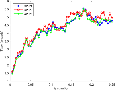
(a) Time

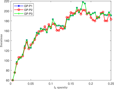
(b) Iterations

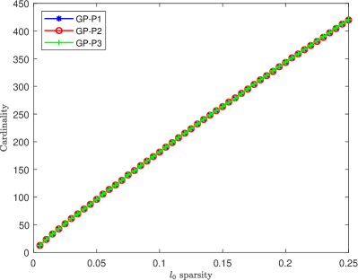
(c) Cardinality

(d) PEV

Figure 2: Comparing the solution quality and efficiency of GPSPCA under (P1), (P2) and (P3) subproblems

Figure 2 depicts the the solution quality and efficiency of GPSPCA algorithm under (P1), (P2) and (P3) subproblems in four aspects: time, iterations, cardinality and PEV. From Figure 2 we see that the cardinality and PEV of GP-P1, GP-P2, GP-P3 are the same. The running time and iterations of GP-P1, GP-P2 and GP-P3 are both close. The simulation results confirm the conclusions in Theorem 8 and Remark 6.

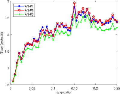
(a) Time

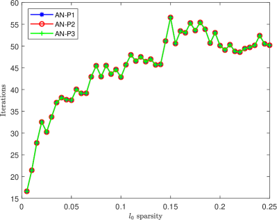
(b) Iterations

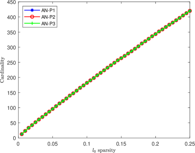
(c) Cardinality

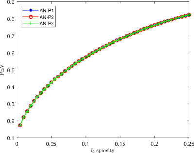
(d) PEV

Figure 3: Comparing the solution quality and efficiency of ANSPCA algorithm under (P1), (P2) and (P3) subproblems

Figure 3 depicts the the solution quality and efficiency of ANSPCA algorithm under (P1), (P2) and (P3) subproblems in four aspects: time, iterations, cardinality and PEV. From Figure 3 we find that AN-P1, AN-P2 and AN-P3 are the same in iterations, cardinality and PEV on this random data. The the running time of AN-P1 and AN-P2 are almost identical, only the time of AN-P3 is a faster than that of AN-P1 and AN-P2. The simulation results again confirm the conclusions in Theorem 8 and Remark 6. In addition, we also see that ANSPCA is faster than GPSPCA.

In the second scenario, we consider problems with two aspects of matrix dimensions: a fixed aspect ratio $n/m=10$, and $m$ is fixed at 500 with exponentially increasing values of $n$. One one hand, we compare the solving speed of GPSPCA algorithms and ANSPCA algorithms using different root-finding methods QASB and MBNW. One the other hand, we compare the speed of different constrained algorithms, including our GPSPCA and ANSPCA algorithms, the $\ell_{1}$ constrained BCD-SPCA${}_{\ell_{1}}$ approach and the $\ell_{0}$ constrained GPBB method. We test 20 times and calculate the average computational time for the extraction of one component (in seconds), which does not include the previous grid search time. We set the sparsity of the first PC extracted to be 5%.

Table 3: The solving speed comparison of GPSPCA algorithms using QASB and MBNW on randomly generated data (in seconds)

data type		GP-P1		GP-P2		GP-P3
$m\times n$		QASB	MBNW	QASB	MBNW	QASB	MBNW
fixed	50$\times$ 500	0.308397	0.327854	0.331808	0.366282	0.337879	0.322534
	100$\times$ 1000	2.132832	2.189169	2.187798	2.153109	2.164093	2.151013
ratio	250$\times$ 2500	25.58315	26.47907	24.88320	25.62218	26.07516	27.09347
	500$\times$ 5000	183.4729	169.2849	130.0196	173.3252	128.2240	173.5543
fixed	500$\times$ 1000	4.015903	3.459357	3.564481	3.42602	3.637700	3.271709
	500$\times$ 2000	16.77741	15.42404	24.74756	14.9727	28.04621	14.33637
$m$	500$\times$ 4000	70.75651	72.49584	68.75089	63.50284	70.57156	69.6927
	500$\times$ 8000	388.6450	402.7237	327.9052	334.3564	415.8329	379.2411

Table 4: The solving speed comparison of ANSPCA algorithms using QASB and MBNW on randomly generated data (in seconds)

data type		AN-P1		AN-P2		AN-P3
$m\times n$		QASB	MBNW	QASB	MBNW	QASB	MBNW
fixed	50$\times$ 500	0.119684	0.127204	0.131323	0.132342	0.132788	0.138747
	100$\times$ 1000	0.957397	0.793248	0.798939	0.795759	0.803481	0.782079
ratio	250$\times$ 2500	9.640766	9.77008	9.378457	10.70906	9.179317	10.07841
	500$\times$ 5000	55.33223	55.57574	48.50123	47.22174	48.62178	56.18631
fixed	500$\times$ 1000	0.963369	0.987795	0.982426	0.899332	1.004097	1.003262
	500$\times$ 2000	7.640022	6.446468	9.923623	6.485785	7.583189	6.574288
$m$	500$\times$ 4000	29.68470	30.18264	29.76016	29.76110	30.76611	29.86022
	500$\times$ 8000	184.6442	216.8571	168.6180	182.6167	168.8092	196.2983

Table 3 and Table 4 show the solving speed of three GPSPCA algorithms and three ANSPCA algorithms using QASB and MBNW, respectively. From Table 3 and Table 4 we see that the solving speed of GPSPCA and ANSPCA algorithms by using QASB and MBNW methods are close, QASB is a little bit faster than MBNW in most cases on large-scale data.

Table 5: The solving speed comparison of different constrained algorithms for a fixed aspect ratio $n/m=10$ (in seconds)

$m\times n$	50$\times$ 500	100$\times$ 1000	500$\times$ 5000	250$\times$ 2500
GP-P1	0.30839732	2.132832394	25.58315448	183.4728864
GP-P2	0.331808416	2.187797667	24.88320128	130.0195649
GP-P3	0.337878505	2.164093439	26.07516253	128.2240166
AN-P1	0.11968432	0.957396717	9.640765565	55.33222742
AN-P2	0.131323195	0.798939172	9.37845674	48.50123347
AN-P3	0.13278835	0.803481061	9.17931745	48.62177537
BCDSPCA${}_{\ell_{1}}$	0.41100588	2.69379707	38.94466327	198.3588296
GPBB	0.32659681	2.07800291	21.48982195	74.15772227

Table 6: The solving speed comparison of different constrained algorithms for $m$ is fixed at 500 (in seconds)

$m\times n$	500$\times$ 1000	500$\times$ 2000	500$\times$ 4000	500$\times$ 8000
GP-P1	4.015903385	16.7774142	70.75651123	388.644996
GP-P2	3.56448103	24.74755891	68.75088813	327.9051987
GP-P3	3.63770008	28.046205	70.57155305	415.8329173
AN-P1	0.96336885	7.640021525	29.68469773	184.6441526
AN-P2	0.9824258	9.923623106	29.76016001	168.6180109
AN-P3	1.004097328	7.583189344	30.76611231	168.8091549
BCDSPCA${}_{\ell_{1}}$	7.2781	27.68084787	136.8822897	471.04013
GPBB	2.500841875	14.11177175	53.84681762	184.9348276

Table 5 and Table 6 further compare the solving speed of different constrained algorithms, including our GPSPCA and ANSPCA algorithms (using QASB root-finding method), the $\ell_{1}$ constrained BCD-SPCA${}_{\ell_{1}}$ approach and the $\ell_{0}$ constrained GPBB method. One also sees that there are no obvious difference among GP-P1, GP-P2, GP-P3 algorithms, among AN-P1, AN-P2 and AN-P3 algorithms, but ANSPCA is much faster than GPSPCA as a whole. ANSPCA is the fastest constrained algorithm, GPBB is the second, and BCDSPCA${}_{\ell_{1}}$ is the slowest maybe due to the ordering process.

5.3.3 Convergence test of the proposed ANSPCA algorithm

In these simulations, we will test the convergence result (ii) in Theorem 14. We randomly generate $50\times 200$ and $500\times 200$ data matrixes $A$ with mean 0 and standard deviation 1, and use the same parameters $\mu=-0.1$, $\sigma=0.25$ with that in Hager et al. (2016), and also set $M$ to be 50, 6, 1, respectively. The change of the errors $\|{\bm{x}}^{j+1}-{\bm{x}}^{j}\|_{2}$ with the iterations are depicted in Figure 4 and Figure 5 for AN-P1, AN-P2, AN-P3 algorithms.

(a) AN-P1

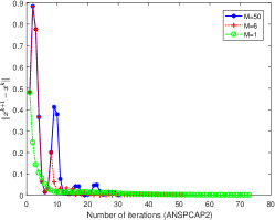
(b) AN-P2

(c) AN-P3

Figure 4: The change of $\|{\bm{x}}^{j+1}-{\bm{x}}^{j}\|_{2}$ with the iterations of ANSPCA algorithm for $50\times 200$ data matrix

(a) AN-P1

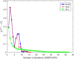
(b) AN-P2

(c) AN-P3

Figure 5: The change of $\|{\bm{x}}^{j+1}-{\bm{x}}^{j}\|_{2}$ with the iterations of ANSPCA algorithms for $500\times 200$ data matrix

From Figure 4 and Figure 5, we see that three ANSPCA algorithms AN-P1, AN-P2, AN-P3 can all converge quickly, especially when taking a large $M$.

5.4 Experiments on real data

In this subsection, we compare our GPSPCA and ANSPCA algorithms with the $\ell_{0}$ constrained GPBB method and the $\ell_{1}$ penalized ConGradU, Gpower${}_{\ell_{1}}$ algorithms on three real datasets: Pitprops data, 20 newsgroups data and ColonCancer data.

5.4.1 Pitprops dataset

The Pitprops dataset, which stores 180 observations of 13 variables, was first introduced by Jeffers Jeffers et al. (1967) to show the difficulty of interpreting PCs. This dataset has been a standard benchmark to evaluate algorithms for sparse PCA.

In these experiments, for each utilized method, 6 sparse PCs were extracted with cardinality setting: 7-2-3-1-1-1 Zhao et al. (2015), 7-2-4-7-2-3 and 12-6-5-4-3-2 Lu and Zhang (2012), and so that the $\ell_{0}$ sparsity for GPBB is about 0.19, 0.32 and 0.41. The $\ell_{1}$ norm parameters $t$ of GPSPCA, ANSPCA and BCD-SPCA are taken to be [2.5 1.1 1.43 1.0002 1.0002 1.0002], [2.51 1.1 1.565 2.3 1.03 1.3] and [2.95 1.895 1.23 1.5 1.02 1.03] (which are near [$\sqrt{7}~{}\sqrt{2}~{}\sqrt{3}$ 1 1 1], [$\sqrt{7}~{}\sqrt{2}~{}\sqrt{4}~{}\sqrt{7}~{}\sqrt{2}~{}\sqrt{3}$], [$\sqrt{12}~{}\sqrt{6}~{}\sqrt{5}~{}\sqrt{4}~{}\sqrt{3}~{}\sqrt{2}$]), respectively. Through the time-consuming grid search to get the penalized parameters of $\ell_{1}$ norm for ConGradU and Gpower${}_{\ell_{1}}$. In GPSPCA, taking the lower bound $\alpha_{\min}=0.1$ and upper bound $\alpha_{\max}=2$ of BB step size, and the tolerance error $\varepsilon_{GP}=1\hbox{e}-6$; In ANSPCA, taking the lower bound $\alpha_{\min}=-1\hbox{e}+7$ and upper bound $\alpha_{\max}=-0.1$ of BB step size, the tolerance error $\varepsilon_{AN}=1\hbox{e}-6$, and set $M=50$ and $\sigma=0.25$ same as in Hager et al. (2016). QASB root-finding method is used in GPSPCA and ANSPCA algorithms

Table 7: The experimental results of GPSPCA and ANSPCA for Pitprops data with cardinality setting 7-2-3-1-1-1

	GP-P1	GP-P2	GP-P3	AN-P1	AN-P2	AN-P3
sparsity	0.192308	0.192308	0.192308	0.192308	0.192308	0.192308
non-ortho	1.487547	1.489458	1.487547	1.494750	1.494750	1.494750
correlation	0.177564	0.177564	0.177564	0.177564	0.177564	0.177564
PEV(%)	72.55638	72.55643	72.55638	72.55643	72.55643	72.55643
RRE	0.493909	0.493912	0.493909	0.493918	0.493918	0.493918

Table 8: The experimental results of GPSPCA and ANSPCA for Pitprops data with cardinality setting 7-2-4-7-2-3

	GP-P1	GP-P2	GP-P3	AN-P1	AN-P2	AN-P3
sparsity	0.320513	0.320513	0.320513	0.320513	0.320513	0.320513
non-ortho	13.08575	13.10793	13.08575	13.26145	13.26054	13.26145
correlation	0.527682	0.528138	0.527682	0.527163	0.527096	0.527163
PEV(%)	77.31753	77.31772	77.31753	77.37516	77.37478	77.37516
RRE	0.429477	0.429470	0.429477	0.429211	0.429221	0.429211

Table 9: The experimental results of GPSPCA and ANSPCA for Pitprops data with cardinality setting 12-6-5-4-3-2

	GP-P1	GP-P2	GP-P3	AN-P1	AN-P2	AN-P3
sparsity	0.410256	0.410256	0.410256	0.410256	0.410256	0.410256
non-ortho	13.96281	13.91463	13.96281	13.92773	13.92800	13.92773
correlation	0.379617	0.379042	0.379617	0.378628	0.378633	0.378628
PEV(%)	77.93167	77.93172	77.93167	78.17187	78.17187	78.17187
RRE	0.446316	0.446335	0.446316	0.442817	0.442817	0.442817

Table 7-9 presents the performance index results of GPSPCA and ANSPCA for SCoTLASS problems (SPCA-P1), (SPCA-P2) and (SPCA-P3) with three cardinality settings: 7-2-3-1-1-1, 7-2-4-7-2-3 and 12-6-5-4-3-2, respectively. From them, one also sees that the results of GPSPCA and ANSPCA for (P1) and (P3) subproblems are the same. There is no obvious difference between (P2) and (P1) (or (P3)) subproblems. This again confirm the conclusions in Theorem 8 and Remark 6.

Table 10: The experimental results of all 6 considered algorithms for Pitprops data with cardinality setting 7-2-3-1-1-1

	GP-P3	AN-P3	BCD-SPCA${}_{\ell_{1}}$	GPBB	ConGradU	Gpower${}_{\ell_{1}}$
sparsity	0.192308	0.192308	0.192308	0.192308	0.192308	0.192308
non-ortho	1.487547	1.494750	4.647480	4.018446	0.776695	12.88813
correlation	0.177564	0.177564	0.157507	0.533711	0.167393	0.664802
PEV(%)	72.55638	72.55643	69.84064	71.74632	72.86088	74.26210
RRE	0.493909	0.493918	0.524715	0.494837	0.491642	0.472651

Table 11: The experimental results of all 6 considered algorithms for Pitprops data with cardinality setting 7-2-4-7-2-3

	GP-P3	AN-P3	BCD-SPCA${}_{\ell_{1}}$	GPBB	ConGradU	Gpower${}_{\ell_{1}}$
sparsity	0.320513	0.320513	0.320513	0.320513	0.320513	0.320513
non-ortho	13.08575	13.26145	17.4116893	8.53104	10.54888	11.56679
correlation	0.527682	0.527163	0.419179	0.533711	0.494277	0.718394
PEV(%)	77.31753	77.37516	70.69511	73.49946	78.32748	80.19115
RRE	0.429477	0.429211	0.461786	0.467493	0.418377	0.397846

Table 12: The experimental results of all 6 considered algorithms for Pitprops data with cardinality setting 12-6-5-4-3-2

	GP-P3	AN-P3	BCD-SPCA${}_{\ell_{1}}$	GPBB	ConGradU	Gpower${}_{\ell_{1}}$
sparsity	0.410256	0.410256	0.410256	0.410256	0.410256	0.410256
non-ortho	13.96281	13.92773	20.69281	15.45535	16.72485	14.28546
correlation	0.379617	0.378628	0.228500	0.495762	0.433502	0.573486
PEV(%)	77.93167	78.17187	77.53197	68.14583	77.54337	78.52479
RRE	0.446316	0.442817	0.399548	0.480160	0.454419	0.425696

Table 10-12 presents the performance index results of all 6 considered algorithms in this paper with three cardinality settings: 7-2-3-1-1-1, 7-2-4-7-2-3 and 12-6-5-4-3-2, respectively. We bold the best indexes in each table. From Table 10-12 we see that although all the performance indexes of our GPSPCA and ANSPCA algorithms are not the best, but the solution quality are close to the best results, which indicate that our algorithms perform stably and fairly on Pitprop data.

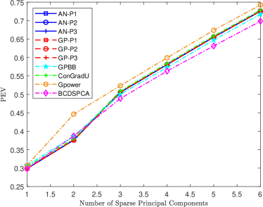
(a) PEVs with cardinality setting 7-2-3-1-1-1

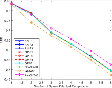
(b) RREs with cardinality setting 7-2-3-1-1-1

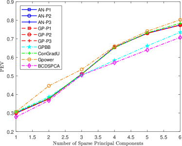
(c) PEVs with cardinality setting 7-2-4-7-2-3

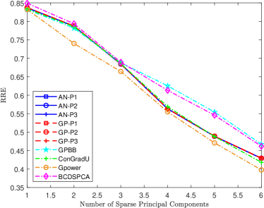
(d) RREs with cardinality setting 7-2-4-7-2-3

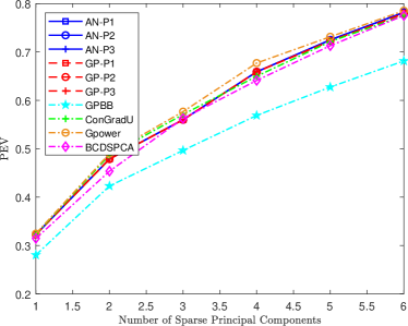
(e) PEVs with cardinality setting 12-6-5-4-3-2

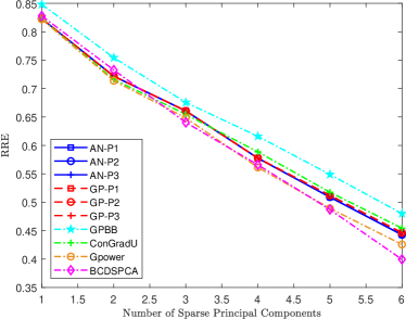
(f) RREs with cardinality setting 12-6-5-4-3-2

Figure 6: The change of PEVs and RREs of GPSPCA, ANSPCA, BCDSPCA${}_{\ell_{1}}$ and GPBB under different different sparse PCs for Pitprops data

Then Figure 6 depicts the change of PEVs and RREs under different sparse PCs of all 6 considered algorithms with three cardinality settings: 7-2-3-1-1-1, 7-2-4-7-2-3 and 12-6-5-4-3-2 for Pitprops data. From Figure 6 we also see that our algorithms perform stably and fairly on Pitprop data.

5.4.2 20 newsgroups dataset

20 Newsgroups data used in this subsection downloaded from http://cs.

nyu.edu/r̃oweis/data.html. It’s a tiny version of the 20newsgroups data, with binary occurance data for 100 words across 16242 postings (that is, $m=16242,n=100$), which is a typical low-dimension and large-sample data. Sam Roweis have tagged the postings by the highest level domain in the array “newsgroups”.

In these experiments, we set the $\l_{0}$ sparsity parameter $k$ in GPBB to be 12, 26 and 36 so that $\ell_{0}$ sparsity are 0.12, 0.26 and 0.36, respectively, then choose proper $\ell_{1}$ sparsity parameters for other algorithms. In GPSPCA, taking the lower bound $\alpha_{\min}=0.1$ and upper bound $\alpha_{\max}=10000$ of BB step size, and the tolerance error $\varepsilon_{GP}=1\hbox{e}-6$; In ANSPCA, the lower bound $\alpha_{\min}=-1\hbox{e}+7$ and upper bound $\alpha_{\max}=-0.1$ of BB step size, the tolerance error $\varepsilon_{GP}=1\hbox{e}-6$, and set $M=50$ and $\sigma=0.25$ same as in Hager et al. (2016).

Table 13: The experimental results of GPSPCA and ANSPCA for 20 newsgroups data with $\ell_{0}$ sparsity 0.12

	GP-P1	GP-P2	GP-P3	AN-P1	AN-P2	AN-P3
sparsity	0.12	0.12	0.12	0.12	0.12	0.12
non-ortho	0	0	0	0	0	0
correlation	0.088808	0.088842	0.088808	0.088834	0.088689	0.088834
PEV(%)	7.479032	7.479011	7.479032	7.491212	7.491323	7.491212
RRE	0.961729	0.961729	0.961729	0.961665	0.961665	0.961665
time(QASB)	3.291743	3.198999	3.280109	3.324865	3.282968	3.226703
time(MBNW)	3.179126	3.189656	3.289210	3.348138	3.184635	3.235251

Table 14: The experimental results of GPSPCA and ANSPCA for 20 newsgroups data with $\ell_{0}$ sparsity 0.26

	GP-P1	GP-P2	GP-P3	AN-P1	AN-P2	AN-P3
sparsity	0.26	0.26	0.26	0.26	0.26	0.26
non-ortho	0.734292	0.739734	0.734292	0.685473	0.702622	0.685473
correlation	0.073453	0.073635	0.073453	0.071822	0.072387	0.071822
PEV(%)	9.217954	9.217802	9.217954	9.219163	9.218764	9.219163
RRE	0.952703	0.952703	0.952703	0.952699	0.952700	0.952699
time(QASB)	3.113743	3.335577	3.163294	3.122756	3.297714	3.308276
time(MBNW)	3.130384	3.134944	3.041041	3.196795	3.069356	3.126040

Table 15: The experimental results of GPSPCA and ANSPCA for 20 newsgroups data with $\ell_{0}$ sparsity 0.36

	GP-P1	GP-P2	GP-P3	AN-P1	AN-P2	AN-P3
sparsity	0.36	0.36	0.36	0.36	0.36	0.36
non-ortho	1.647439	1.658136	1.647439	1.600600	1.615837	1.600600
correlation	0.069781	0.070007	0.069781	0.068823	0.068698	0.068823
PEV(%)	10.10784	10.10731	10.10784	10.11136	10.12078	10.11136
RRE	0.948046	0.948049	0.948046	0.948029	0.947980	0.948029
time(QASB)	3.2048645	3.240376	3.227912	3.257714	3.389049	3.197513
time(MBNW)	3.223576	3.105585	3.158840	3.148903	3.045804	3.184320

Table 13 - Table 15 present the performance index results of GPSPCA and ANSPCA for SCoTLASS problems (SPCA-P1), (SPCA-P2) and (SPCA-P3) on 20newsgroups with three $\ell_{0}$ sparsity: 0.12, 0.26 and 0.36. We test GPSPCA and ANSPCA algorithms using different root-finding methods QASB and MBNW. Since the solution quality are completely same, we only show the running time (in seconds) of GPSPCA and ANSPCA algorithms using QASB and MBNW in the last two rows, respectively. From Table 13 - Table 15, one also see that the solution quality of GPSPCA and ANSPCA for (P1) and (P3) subproblems are the same, there is no obvious difference between (P2) and (P1) (or (P3)) subproblems. This again confirms the conclusions in Theorem 8 and Remark 6. Moreover, one also observe that ANSPCA is faster than GPSPCA as a whole. MBNW is a little bit faster than QASB on 20 newsgroups data in most cases.

Table 16: The experimental results of all 6 considered algorithms for 20 newsgroups data with $\ell_{0}$ sparsity about 0.12

	GP-P3	AN-P3	BCD-SPCA${}_{\ell_{1}}$	GPBB	ConGradU	Gpower${}_{\ell_{1}}$
sparsity	0.12	0.12	0.12	0.12	0.14	0.13
non-ortho	0	0	0.250713	1.354993	0.060981	0
correlation	0.088808	0.088834	0.130823	0.152435	0.101326	0
PEV(%)	7.479032	7.491212	7.130721	6.298703	8.422297	8.749329
RRE	0.961729	0.961665	0.963391	0.967717	0.956709	0.955057
time(s)	3.280109	3.226703	3.477888	3.375629	3.381738	3.556981

Table 17: The experimental results of all 6 considered algorithms for 20 newsgroups data with $\ell_{0}$ sparsity about 0.26

	GP-P3	AN-P3	BCD-SPCA${}_{\ell_{1}}$	GPBB	ConGradU	Gpower${}_{\ell_{1}}$
sparsity	0.26	0.26	0.245	0.26	0.255	0.26
non-ortho	0.734292	0.685473	0.319142	1.387991	0.210248	2.320208
correlation	0.073453	0.071822	0.068810	0.157896	0.071080	0
PEV(%)	9.217954	9.219163	8.998858	6.338695	9.223777	10.03170
RRE	0.952703	0.952699	0.953850	0.967488	0.952647	0.948459
time(s)	3.163294	3.308276	4.349967	3.516325	5.482299	4.739926

Table 18: The experimental results of all 6 considered algorithms for 20 newsgroups data with $\ell_{0}$ sparsity 0.36

	GP-P3	AN-P3	BCD-SPCA${}_{\ell_{1}}$	GPBB	ConGradU	Gpower${}_{\ell_{1}}$
sparsity	0.36	0.36	0.36	0.36	0.36	0.36
non-ortho	1.647439	1.600600	3.627874	1.404085	1.489592	2.801727
correlation	0.069781	0.068823	0.095851	0.159895	0.066832	0
PEV(%)	10.10784	10.11136	10.11587	6.34829	10.10969	10.40544
RRE	0.948046	0.948029	0.947941	0.967430	0.948041	0.946460
time(s)	3.227912	3.197513	3.441490	3.799539	3.319411	3.139909

Table 16-Table 18 present the performance index results of BCD-SPCA${}_{\ell_{1}}$, GPBB, ConGradU, Gpower${}_{\ell_{1}}$ and our GP-P3 and AN-P3 algorithms (using QASB). We bold the best indexes in the table. As shown in Table 16-Table 18, Gpower${}_{\ell_{1}}$ performs the best on 20newsgroups data; our GPSPCA and ANSPCA algorithms perform fairly on 20newsgroups data. When the sparsity is higher, the solution quality and efficiency of our GPSPCA and ANSPCA algorithms are better.

5.4.3 ColonCancer dataset

ColonCancer dataset is similar to the yeast gene expression dataset. It contains expression levels of 2000 genes taken in 62 different samples (20 normal samples and 42 cancerous sample). For each sample it is indicated whether it came from a tumor biopsy or not.

In these experiments, we will examine the performance of GPSPCA and ANSPCA algorithms for SCoTLASS problems (SPCA-P1), (SPCA-P2) and (SPCA-P3), and compare them with the $\ell_{0}$-constrained GPBB method in Hager et al. (2016) for such high-dimension and small-sample data. Here ten PCs are retained, the $\ell_{0}$ sparsity are set to be 0,025 and 0.05, respectively. In GPSPCA, taking the lower bound $\alpha_{\min}=0.1$ and upper bound $\alpha_{\max}=1\hbox{e}+7$ of BB step size, and the tolerance error $\varepsilon_{GP}=1\hbox{e}-7$; In ANSPCA, the lower bound $\alpha_{\min}=-1\hbox{e}+7$ and upper bound $\alpha_{\max}=-0.1$ of BB step size, the tolerance error $\varepsilon_{AN}=1\hbox{e}-7$, and set $M=50$ and $\sigma=0.25$ same as in Hager et al. (2016).

Table 19: The experimental results of GPSPCA and ANSPCA for ColonCancer data with $\ell_{0}$ sparsity 0.025

	GP-P1	GP-P2	GP-P3	AN-P1	AN-P2	AN-P3
sparsity	0.025	0.025	0.025	0.025	0.025	0.025
non-ortho	9.060925	9.060925	9.060925	8.773778	8.773778	8.773778
correlation	0.656520	0.656520	0.656520	0.652649	0.652649	0.652649
PEV(%)	44.60294	44.60294	44.60294	44.55103	44.55103	44.55103
RRE	0.658404	0.658404	0.658404	0.658836	0.658836	0.658836
time(QASB)	14.17658	13.46575	13.57485	9.2298437	9.389257	9.11774
time(MBNW)	14.78742	13.85781	13.95844	9.4749378	9.625218	9.54209

Table 20: The experimental results of GPSPCA and ANSPCA for ColonCancer data with $\ell_{0}$ sparsity 0.05

	GP-P1	GP-P2	GP-P3	AN-P1	AN-P2	AN-P3
sparsity	0.05	0.05	0.05	0.05	0.05	0.05
non-ortho	7.960083	7.960083	7.960083	7.886136	7.886136	7.886136
correlation	0.707783	0.707783	0.707783	0.707460	0.707460	0.707460
PEV(%)	53.67847	53.67847	53.67847	53.67487	53.67487	53.67487
RRE	0.605869	0.605869	0.605869	0.605950	0.605950	0.605950
time(QASB)	19.83169	18.93937	18.92147	15.09567	15.73355	15.07514
time(MBNW)	22.76613	19.65183	19.70344	15.42362	17.81128	16.87169

Table 19 and Table 20 present the performance index results of GPSPCA and ANSPCA for SCoTLASS problems (SPCA-P1), (SPCA-P2) and (SPCA-P3) on ColonCancer data with two $\ell_{0}$ sparsity: 0.025, and 0.05. We also test GPSPCA and ANSPCA algorithms using different root-finding methods QASB and MBNW. The solution quality are still completely same, we also show the running time (in seconds) of GPSPCA and ANSPCA algorithms using QASB and MBNW in the last two rows, respectively. From Table 19 and Table 20, one see that the solution quality of GPSPCA and ANSPCA for (P1), (P2) and (P3) subproblems are the same for very small $t$. This again confirms the conclusions in Theorem 8 and Remark 6. Moreover, one also observe that ANSPCA is faster than GPSPCA as a whole. As shown in Table 3 and Table 4, QASB is a little bit faster than MBNW on ColonCancer data.

Table 21: The experimental results of 5 considered algorithms for ColonCancer data with $\ell_{0}$ sparsity about 0.025

	GP-P3	AN-P3	BCD-SPCA${}_{\ell_{1}}$	GPBB	Gpower${}_{\ell_{1}}$
sparsity	0.025	0.025	0.0252	0.025	0.025
non-ortho	9.060925	8.773778	87.108222	43.451939	9.437723
correlation	0.656520	0.652649	0.995545	0.912070	0.430196
PEV(%)	44.60294	44.55103	11.51628	45.40040	47.68198
RRE	0.658404	0.658836	0.626347	0.629980	0.630322
time(s)	13.574848	9.117742	581.309018	44.457744	8.8651

Table 22: The experimental results of 5 considered algorithms for ColonCancer data with $\ell_{0}$ sparsity about 0.05

	GP-P3	AN-P3	BCD-SPCA${}_{\ell_{1}}$	GPBB	Gpower${}_{\ell_{1}}$
sparsity	0.05	0.05	0.05015	0.05	0.05005
non-ortho	7.960083	7.886136	86.460665	38.650985	6.123612
correlation	0.707783	0.707460	0.998639	0.842065	0.131793
PEV(%)	53.67847	53.67487	17.21433	53.16904	66.59446
RRE	0.605869	0.605950	0.568248	0.576578	0.564061
time(s)	18.921469	15.075141	325.143882	66.982931	9.697913

Table 21 and Table 22 present the performance index results of BCD-SPCA${}_{\ell_{1}}$, GPBB, Gpower${}_{\ell_{1}}$ and our GP-P3 and AN-P3 algorithms (using QASB) with two $\ell_{0}$ sparsity: 0.025 and 0.05 on ColonCancer data. We bold the best indexes in the table. As shown in Table 21 and Table 22, Gpower${}_{\ell_{1}}$ performs the best on ColonCancer data; our GPSPCA and ANSPCA algorithms perform well and stably on ColonCancer data, especially they are faster than the other two constrained BCD-SPCA${}_{\ell_{1}}$, GPBB algorithms.

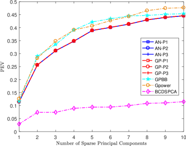
(a) PEV with $\ell_{0}$ sparsity 0.025

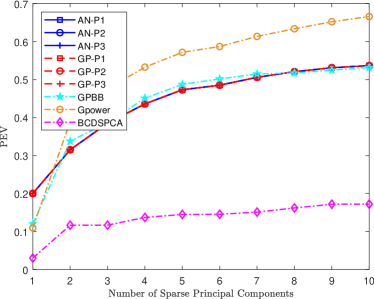
(b) PEV with $\ell_{0}$ sparsity 0.05

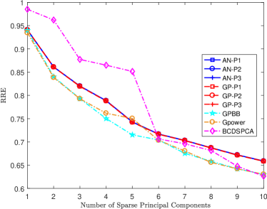
(c) RRE with $\ell_{0}$ sparsity 0.025

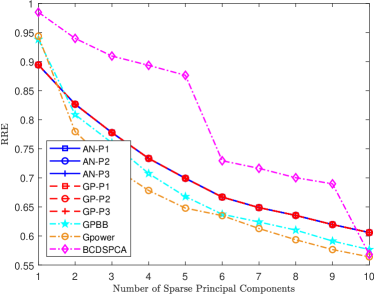
(d) RRE with $\ell_{0}$ sparsity 0.05

Figure 7: The change of PEV and RRE with different numbers of sparse PCs for GPSPCA, ANSPCA, BCDSPCA${}_{\ell_{1}}$, GPBB and Gpower${}_{\ell_{1}}$ on ColonCancer data

Figure 7 further depicts the change of PEV and RRE with different numbers of sparse PCs for GPSPCA, ANSPCA, BCDSPCA${}_{\ell_{1}}$, GPBB and Gpower${}_{\ell_{1}}$ on ColonCancer data. From Figure 7 we see that PEV increases and RRE decreases with growth of the numbers of sparse PCs. Same as shown in Table 21 and Table 22, Gpower${}_{\ell_{1}}$ performs the best on ColonCancer data; our GPSPCA and ANSPCA algorithms perform well on ColonCancer data.

As a whole, through comparing the proposed GPSPCA and ANSPCA algorithms for SCoTLASS problems (SPCA-P1), (SPCA-P2) and (SPCA-P3) with the present typical algorithms GPBB, BCDSPCA${}_{\ell_{1}}$, ConGradU and Gpower${}_{\ell_{1}}$ on three typical real dataset, we find that our proposed algorithms GPSPCA and ANSPCA for three SCoTLASS problems perform stably, are faster than the other two constrained algorithms BCD-SPCA${}_{\ell_{1}}$ and GPBB on the large-scale dataset. Although our GPSPCA and ANSPCA algorithms did not perform the best, the $\ell_{1}$ sparse parameters are easy to be set since the initial vector can be chosen simply, and the (P1), (P2) and (P3) subproblems have analytic solutions, the proposed GPSPCA and ANSPCA algorithms can be all computed efficiently, and used for large-scale computation. From the experimental results we also see that Gpower${}_{\ell_{1}}$ perform the best in solution quality and efficiency, however, its penalized parameters are difficult to be chosen, and one need to spend much longer time to find them.

6 Conclusions

In this paper, we employed the projection method onto the intersection of an $\ell_{1}$ ball/sphere and an $\ell_{2}$ ball/sphere proposed in Liu et al. (2020), designed a gradient projection method (GPSPCA for short) and an approximate Newton algorithm (ANSPCA for short) for three SCoTLASS problems (SPCA-P1), (SPCA-P2) and (SPCA-P3), and proved the global convergence for them. We showed the equivalence of the solution to SPCA-P1 and SPCA-P3, and the solution to SPCA-P2 and SPCA-P3 are the same in most case. We conducted several numerical experiments in MATLAB environment to exmine the performance of our proposed GPSPCA and ANSPCA algorithms. The simulation results confirmed the conclusions in Theorem 8 and Remark 6, and showed that ANSPCA was faster than GPSPCA on large-scale data. Compare to the typical SPCA algorithms GPBB Hager et al. (2016), BCDSPCA${}_{\ell_{1}}$ Zhao et al. (2015), ConGradU Witten et al. (2009) and Gpower${}_{\ell_{1}}$ Journée et al. (2010), the proposed GPSPCA and ANSPCA algorithms performed fairly well and stably, and highly efficient for large-scale computation.

References

References

• Jolliffe (2002) I. T. Jolliffe, Principal Component Analysis, 2nd ed., Springer, New York, 2002.
• Jolliffe et al. (2003) I. T. Jolliffe, N. T. Trendafilov, M. Uddin, A modified principal component technique based on the LASSO, Journal of computational and Graphical Statistics 12 (3) (2003) 531–547.
• Liu et al. (2020) H. Liu, H. Wang, M. Song, Projections onto the Intersection of a One-Norm Ball or Sphere and a Two-Norm Ball or Sphere, Journal of Optimization Theory and Applications 187 (2020) 520–534.
• Trendafilov and Jolliffe (2006) N. T. Trendafilov, I. T. Jolliffe, Projected gradient approach to the numerical solution of the SCoTLASS, Computational Statistics & Data Analysis 50 (2006) 242–253.
• Witten et al. (2009) D. M. Witten, R. Tibshirani, T. Hastie, A penalized matrix decomposition, with applications to sparse principal components and canonical correlation analysis, Biostatistics 10 (3) (2009) 515–534.
• Zou et al. (2006) H. Zou, T. Hastie, R. Tibshirani, Sparse principal component analysis, Journal of computational and graphical statistics 15 (2) (2006) 265–286.
• Shen and Huang (2008) H. Shen, J. Z. Huang, Sparse principal component analysis via regularized low rank matrix approximation, Journal of Multivariate Analysis 99 (2008) 1015–1034.
• d’Aspremont et al. (2008) A. d’Aspremont, F. Bach, L. E. Ghaoui, Optimal solutions for sparse principal component analysis, Journal of Machine Learning Research 9 (2008) 1269–1294.
• Journée et al. (2010) M. Journée, Y. Nesterov, P. Richtárik, R. Sepulchre, Generalized power method for sparse principal component analysis, J. Mach. Learn. Res. 11 (2010) 517–553.
• d’Aspremont et al. (2005) A. d’Aspremont, L. E. Ghaoui, M. I. Jordan, G. R. Lanckriet, A direct formulation for sparse PCA using semidefinite programming, in: Advances in neural information processing systems, 41–48, 2005.
• Luss and Teboulle (2011) R. Luss, M. Teboulle, Convex approximations to sparse PCA via Lagrangian duality, Operations Research Letters 39 (1) (2011) 57–61.
• Sigg and Buhmann (2008) C. Sigg, J. Buhmann, Expectation-maximization for sparse and non-negative PCA, in: Machine Learning, Proceedings of the Twenty-Fifth International Conference (ICML 2008), 960–967, doi:10.1145/1390156.1390277, 2008.
• Luss and Teboulle (2013) R. Luss, M. Teboulle, Conditional gradient algorithmsfor rank-one matrix approximations with a sparsity constraint, SIAM Review 55 (1) (2013) 65–98.
• Lu and Zhang (2012) Z. Lu, Y. Zhang, An augmented Lagrangian approach for sparse principal component analysis, Mathematical Programming, Series A 135 (2012) 149–193.
• Zhao et al. (2015) Q. Zhao, D. Meng, Z. Xu, C. Gao, A block coordinate descent approach for sparse principal component analysis., Neurocomputing 153 (2015) 180–190.
• Yang (2017) Q. Yang, The block algorithm study for sparse principal component analysis, Master’s thesis, Beihang University, Beijing, P. R. China, 2017.
• Bertsimas and Kitane (2022) D. Bertsimas, D. L. Kitane, Sparse PCA: a geometric approach, Journal of Machine Learning Research 23 (2022) 1–33.
• Hager et al. (2016) W. W. Hager, D. T. Phan, J. Zhu, Projection algorithms for nonconvex minimization with application to sparse principal component analysis, Jouranl of Global Optimization 65 (2016) 657–676.
• Bertsekas (1976) D. Bertsekas, On the Goldstein-Levitin-Polyak gradient projection method, IEEE Transactions on automatic control 21 (2) (1976) 174–184.
• Barzilai and Borwein (1988) J. Barzilai, J. M. Borwein, Two-point step size gradient methods, IMA journal of numerical analysis 8 (1) (1988) 141–148.
• Birgin et al. (2000) E. G. Birgin, J. M. Martínez, M. Raydan, Nonmonotone spectral projected gradient methods on convex sets, SIAM Journal on Optimization 10 (4) (2000) 1196–1211.
• Figueiredo et al. (2007) M. A. Figueiredo, R. D. Nowak, S. J. Wright, Gradient projection for sparse reconstruction: Application to compressed sensing and other inverse problems, IEEE Journal of selected topics in signal processing 1 (4) (2007) 586–597.
• Wright et al. (2009) S. J. Wright, R. D. Nowak, M. A. Figueiredo, Sparse reconstruction by separable approximation, IEEE Transactions on Signal Processing 57 (7) (2009) 2479–2493.
• Bottou (2010) L. Bottou, Large-scale machine learning with stochastic gradient descent, in: Proceedings of COMPSTAT’2010, Springer, 177–186, 2010.
• Cevher et al. (2014) V. Cevher, S. Becker, M. Schmidt, Convex optimization for big data: Scalable, randomized, and parallel algorithms for big data analytics, IEEE Signal Processing Magazine 31 (5) (2014) 32–43.
• Thom et al. (2015) M. Thom, M. Rapp, G. Palm, Efficient dictionary learning with sparseness-enforcing projections, International Journal of Computer Vision 114 (2-3) (2015) 168–194.
• Duchi et al. (2008) J. Duchi, S. Shalev-Shwartz, Y. Singer, T. Chandra, Efficient projections onto the $\ell_{1}$-ball for learning in high dimensions, Proceedings of the 25th International Conference on Machine Learning (2008) 272–279doi:10.1145/1390156.1390191.
• Liu and Ye (2009) J. Liu, J. Ye, Efficient Euclidean projections in linear time, in: Proceedings of the 26th Annual International Conference on Machine Learning, ACM, 657–664, 2009.
• Songsiri (2011) J. Songsiri, Projection onto an $\ell_{1}$-norm ball with application to identification of sparse autoregressive models, in: Asean Symposium on Automatic Control (ASAC), 2011.
• Condat (2016) L. Condat, Fast projection onto the simplex and the $\ell_{1}$ ball, Mathematical Programming 158 (1-2) (2016) 575–585.
• Mackey (2009) L. Mackey, Deflation methods for sparse PCA, Advances in Neural Information Processing Systems 21 (2009) 1017–1024.
• Rockafellar (1972) R. T. Rockafellar, Convex anaysis, 2nd Printing, Princeton University Press, Princeton, New York, 1972.
• Bolte et al. (2014) J. Bolte, S. Sabach, M. Teboulle, Proximal alternating linearized minimization for nonconvex and nonsmooth problems, Mathematical Programming 146 (2014) 459–494, doi:10.1007/s10107-013-0701-9.
• Jeffers et al. (1967) J. Jeffers, R. Chandler, P. Smith, Two case studies in the application of principal component analysis, Journal of the Royal Statistical Society Series C 16 (3) (1967) 225–236.