Inflation with shallow dip and primordial black holes

Abstract

Primordial black holes may arise through ultra slow-roll inflation. In this work we study a toy model of ultra slow-roll inflation with a shallow dip. The ultra slow-roll stage enhances the curvature perturbations and thus the primordial scalar power spectrum. We analyze the features of the power spectrum numerically and analytically, and then give a rough estimate of the lower and upper bound of the enhancement. These large perturbations also produce second order gravitational waves, which are in the scope of future observations.

I Introduction

Inflationary cosmology has great success in solving the puzzles of standard big bang theory. In addition, it provides elegant explanations for the temperature fluctuations of the cosmic microwave background (CMB) and the seeds for large scale structure (LSS) formation. Present observations of CMB [1] and LSS [2] have significantly constrained inflation on large scales. However, the constraints on small scales are much more weaker, leaving the details of inflationary dynamics on these scales unknown.

A bold but intriguing postulation is that primordial black holes (PBHs) may arise in very early universe [3, 4, 5]. These black holes are a type of hypothetical objects formed from the collapse of overdense region caused by large perturbations on small scales. Due to the primordial origin, they have a wide range of mass down to $\sim 10^{-5}$ g and up to as heavy as supermassive black holes. The PBHs lighter than $\sim 10^{15}$g have evaporated through Hawking radiation, while those heavier still survive at present epoch. These relic PBHs are natural dark matter candidate because they are collision-less and friction-less. They are also considered as the sources of the gravitational wave signals observed by LIGO/Virgo/KAGRA [6, 7, 8, 9, 10, 11, 12, 13, 14, 15, 16, 17, 18, 19, 20, 21]. Current data from various channels of observations have imposed severe constraints on the mass (energy) fraction of PBHs [22, 23, 24, 25, 26, 27, 28, 29, 30, 31, 32, 33, 34, 35, 36, 37, 38, 39, 40]. For example, the mass range $10^{5}-10^{12}~{}M_{\odot}$ is strongly limited by the spectral distortion of the CMB [41, 42, 43, 44], the range $10^{-13}-10^{-5}~{}M_{\odot}$ by gravitational lensing [28, 45, 46], and the range $10^{-3}-1~{}M_{\odot}$ by Pulsar Timing Arrays [47], etc. In most mass windows, the fraction of PBHs as dark matter is less than $1\%$. However, there is still an asteroid mass window, $10^{-16}-10^{-13}~{}M_{\odot}$, in which the PBHs could contribute a large fraction or the total of dark matter.

The most commonly considered mechanism of generating the large perturbations required for PBH formation is inflation, which provides the origin of the primordial quantum fluctuations naturally. To have the PBHs formed, the curvature perturbations need to be enhanced sufficiently. For gaussian distributed curvature perturbations, the primordial scalar power spectrum at scales related to the PBH formation is required to be roughly seven orders larger than that at CMB scales [48]. This may change if the details like non-Gaussianities and non-linear effects are considered [49, 50, 51, 52, 53, 54, 55, 56, 57, 58, 59, 60, 61, 62, 63, 64, 65, 66, 67]. The enhancement can be realised in various inflation models, of which one of the simplest is the single field inflation with an ultra slow-roll (USR) stage. Usually, the USR phase appears if the potential has, for instance, a quasi-inflection point [22, 68, 69, 70, 71, 72, 72, 73, 74, 75], a local minimum/maximum [76, 77, 78, 52, 79, 80, 81, 82], etc. When the inflaton rolls over these features, the slow roll phase transitions to be USR and the inflaton is largely decelerated. In such a stage the curvature perturbations and the primordial power spectrum would be amplified. The PBHs may form after these amplified perturbations re-enter the horizon, provided that the enhancement is sufficient and the USR phase is long enough. The enhancement mechanism is also widely studied in inflation models constructed with piecewise potentials [83, 84, 85, 86]. This type of theories are useful to show the details of the amplification mechanism. However, the non-smooth features may lead to sharp and instantaneous transitions. As is discussed recently [87, 88, 89, 90, 91, 92, 93, 94, 95], such transitions may have significant loop corrections from the small scales to the power spectrum at large scales and spoil the CMB observations. Hence it is of great importance to consider smooth and more realistic models. One may also consider non-standard theories like non-canonical scalar field [96, 97, 98, 99, 100, 101, 102, 103], modified gravity [104, 105, 106, 107, 108], multi-field inflation [109, 110, 111, 112, 113, 114], etc.

In this work we consider the non-monotonic model proposed in [82]. The potential has a shallow dip, with a local minimum and a local maximum. We study the primordial power spectrum both numerically and analytically. In particular, we try to improve the analytical expression of the power spectrum. The analytical description of the power spectrum [115, 116, 117, 118, 119, 81] is meaningful since it relates the model parameters or the slow-roll parameters to the PBH abundance directly. It would be instructive for model building if the analytical expression is highly precise. We also study the second order gravitational waves (GWs) produced by the large perturbations [120, 121, 122, 123, 124, 125, 126, 127]. These GWs are in the scope of future observatories. The detection of stochastic GWs background would imply new physics of the universe. However, the non-detection would also impose strong constraints on the early universe.

This paper is organized as follows. We first introduce the model briefly in section II, then we solve the perturbations and give the numerical and analytical power spectrum in section III. The PBH formation and the induced gravitational waves are considered in section IV and V, respectively. The summary is given in the final section.

II The model

The model proposed in [82] contains two parts,

$$V(\phi)=\alpha\frac{f_{1}(\phi)}{1+f_{1}(\phi)}+\xi\frac{f_{2}(\phi)}{1+f_{2}(\phi)},$$ (1)

where $f_{1}=\frac{1}{4}\lambda\phi^{2}\left((\phi-\upsilon_{1})^{2}+\upsilon_{2}^{2}\right)$ and $f_{2}=\phi^{4}/\upsilon_{3}^{4}$. The first term of the potential features a local minimum, which makes the inflaton undergo an USR period. The second term is the usual slow-roll inflation potential and predicts the CMB observables on large scales. Hence, we require $\xi\gg\alpha$ so that our theory is consistent with CMB observations.

The field equation of the inflaton is

$$\ddot{\phi}+3H\dot{\phi}+V_{,\phi}=0,$$ (2)

where dot represents time derivative. One may also write this equation with the e-folding number,

$$\phi_{,NN}+3\phi_{,N}-\frac{1}{2}\phi_{,N}^{3}+\left(3-\frac{1}{2}\phi_{,N}^{2}\right)\frac{V_{,\phi}}{V}=0.$$ (3)

Defining the slow-roll parameter,

$$\epsilon\equiv-\frac{\dot{H}}{H^{2}}=-\frac{1}{2}\phi_{,N}^{2},\quad\eta\equiv\frac{\dot{\epsilon}}{H\epsilon}=2\frac{\phi_{,NN}}{\phi_{,N}},$$ (4)

the evolution equation (3) then becomes

$$\eta=-2(3-\epsilon)\left(1\pm\sqrt{\frac{\epsilon_{V}}{\epsilon}}\right),$$ (5)

where

$$\epsilon_{V}=\frac{1}{2}\left(\frac{V_{,\phi}}{V}\right)^{2}$$ (6)

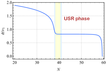
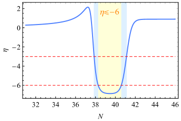
is the potential slow-roll parameter. The “$\pm$” sign appears because of the nonmonotonicity of the potential in our theory. For the usual slow-roll inflation, the potential is monotonic (for inflation period) and $V_{\phi}$ is always positive (or negative) in inflation phase. For USR inflation with a quasi-inflection point (but still monotonic), the potential is extremely flat and the slope $V_{,\phi}\simeq 0$. Equation (5) has a “$-$” sign and straightforwardly gives $\eta\simeq-6$ around the plateau. In our theory, equation (5) has “$-$” sign before the inflaton rolls down to the local minimum. After the inflaton passes through the local minimum, equation (5) has a “$+$” sign before the local maximum. In this period we have $\eta<-6$. This can be shown by the evolution of $\eta$ in Fig. 1.

Figure 1: The evolution of the inflaton (upper) and the slow-roll parameters (lower) for parameter set $P_{1}$ in Table 1. The yellow region represents the USR stage with $\eta\leq-6$, while the region with $\eta\leq-3$ are shaded blue.

Sets	$\phi_{\text{CMB}}[M_{p}]$	$\alpha[M_{p}^{4}]$	$\xi[M_{p}^{4}]$	$\upsilon_{1}[M_{p}]$	$\upsilon_{2}[M_{p}]$	$\upsilon_{3}[M_{p}]$
$P_{1}$	0.1912	$1.425\times 10^{-15}$	$1.425\times 10^{-13}$	$0.094$	$0.02446015$	$0.0099$
$P_{2}$	0.1930	$1.933\times 10^{-15}$	$1.740\times 10^{-13}$	0.096	0.0254076	0.01
$P_{3}$	0.1920	$1.530\times 10^{-15}$	$1.530\times 10^{-15}$	0.095	0.024643	0.01
$P_{4}$	0.1935	$1.530\times 10^{-15}$	$1.530\times 10^{-15}$	0.098	0.02569	0.01

Table 1: Parameter sets used in this paper.

III The curvature perturbations and the power spectrum

III.1 The analytical approach

The USR stage amplifies the curvature perturbations. To be more specific, let us consider the evolution of the curvature perturbations analytically. The evolution equation of the curvature perturbation modes is

$$\mathcal{R}_{k}^{\prime\prime}+(3-\epsilon+\eta)\mathcal{R}_{k}^{\prime}+\frac{k^{2}}{a^{2}H^{2}}\mathcal{R}_{k}=0.$$ (7)

It is also convenient to work in the conformal time coordinate and use the Mukhanov-Sasaki variable. In this work however, we deal with the equation (7) directly. For constant $\epsilon$ and $\eta$, the general solution is

$$\mathcal{R}_{k}(N)=CF^{(1)}_{\nu}\left(\frac{k}{aH}\right)+DF^{(2)}_{\nu}\left(\frac{k}{aH}\right),$$ (8)

where $F^{(1)}_{\alpha}(x)=\left(x/2\right)^{\alpha}J_{-\alpha}(x)\Gamma(1-\alpha)$ and $F^{(2)}_{\alpha}(x)=\left(x/2\right)^{\alpha}J_{\alpha}(x)\Gamma(1+\alpha)$, with $J_{\alpha}(x)$ the Bessel function of the first kind and $\Gamma(x)$ the Gamma function. $C$ and $D$ are coefficients with $k$ dependence, and $\nu=(3-\epsilon+\eta)/2$.

Based on the above observation and the evolution of the slow-roll parameters, we divide the inflation process into four stages, the slow-roll stage ($N<N_{1}$), the USR stage ($N_{1}\leq N<N_{2}$), the constant-roll stage ($N_{2}\leq N<N_{3}$), and the final slow-roll stage ($N_{3}\leq N$). The slow-roll parameter $\epsilon$ will be neglected in the rest of this paper due to its smallness, and the parameter $\eta$ is approximated as

$$\eta\simeq\left\{\begin{array}[]{ll}0,&\hbox{$0\leq N<N_{1}$}\\ \eta_{u},&\hbox{$N_{1}\leq N<N_{2}$}\\ \eta_{c},&\hbox{$N_{2}\leq N<N_{3}$}\\ 0,&\hbox{$N_{3}\leq N$}\end{array}\\ \right..$$ (9)

Note that $N=0$ corresponds to the start of inflation.

Figure 2: Upper: The schematic of the model (9) and its comparison to the numerical $\eta$ (for $P_{1}$ set parameters). The parameters are $N_{2}-N_{1}=2.5$, $\eta_{u}=-6.2$, $N_{3}-N_{2}=18$, and $\eta_{c}=0.9$. The transition $N_{1}\simeq 38.4$ is set such that the predicted dip of the power spectrum coincide with that of the numerical one. Note that the CMB scales exit the horizon at $N_{\text{CMB}}\simeq 9$. Lower: A comparison of the power spectrum obtained by numerical evolution (for parameter set $P_{1}$) and the analytical one constructed in upper panel. The dashed vertical lines correspond to $k_{1}$ (left) and $k_{2}$ (right).

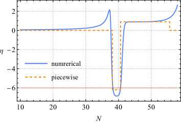
From the numerical evolution of the background quantities in Fig. 1, we see that the slow-roll parameter $\eta$ starts growing and exceeds unity after the constant-roll stage. This certainly violates the slow-roll condition. However, in (9) we assume that for $N\geq N_{3}$ the inflation process turns back to be slow-roll and $\eta\simeq 0$ for simplicity. This approximation is reasonable provided that the constant-roll phase lasts long enough, in which case the scales responsible for PBH production have exited the horizon and being frozen for a long time at $N=N_{3}$, so that they would not be affected by the final stage ($N\geq N_{3}$).

Under this setup we can solve the curvature perturbation modes in each stage analytically. The coefficients are obtained by the continuity conditions at transitions. Finally, the power spectrum in the late time limit ($k\ll aH$) is given by

$$\mathcal{P}_{\mathcal{R}}(k)=\lim_{k\ll aH}\frac{k^{3}}{2\pi^{2}}\big{|}\mathcal{R}^{(3)}_{k}\big{|}^{2}\simeq\frac{k^{3}}{2\pi^{2}}\left|C_{3}\right|^{2}.$$ (10)

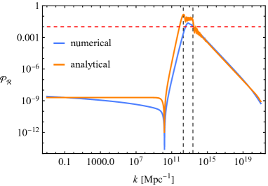
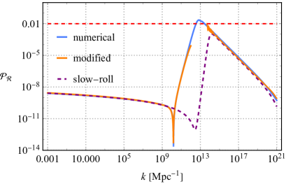
The coefficients are computed in the Apendix. We show the comparison of the numerically calculated power spectrum and the analytical one in Fig. 2. We see that they have some differences. The largest discrepancy is the prediction on large scales that exit the horizon in slow-roll regime ($N\leq N_{1}$). This is because the analytical approach neglected the evolution of the slow-roll parameter $\epsilon$ in deriving the analytical power spectrum (10). To understand this, let us consider the expansion of the power spectrum (10) in $k$,

$$\mathcal{P}_{\mathcal{R}}(k)\simeq\frac{H^{2}}{8\pi^{2}\epsilon_{*}}\Bigg{[}1+c_{2}\left(\frac{k}{k_{1}}\right)^{2}+c_{4}\left(\frac{k}{k_{1}}\right)^{4}$$

$$+c_{6}\left(\frac{k}{k_{1}}\right)^{6}+\mathcal{O}(k^{8})\Bigg{]},$$ (11)

where $\epsilon_{*}$ is evaluated at the time when the CMB pivot scale $k_{*}=0.05~{}\text{Mpc}^{-1}$ exits the horizon, and $k_{1}=a(N_{1})H$ represents the scale that exits the horizon at transition $N=N_{1}$. The coefficients $c_{i}$ are functions of slow-roll parameters and the duration of the each stage of inflation, hence the effects of super-horizon evolution are included in them. This expansion gives a scale invariant power spectrum for scales $k\ll k_{1}$, as is shown in Fig. 2. As a rough modification which includes the evolution of $\epsilon$, we replace the constant parameter $\epsilon_{*}$ by $\epsilon(\tau_{k})$,

Figure 3: The power spectrum computed by different approaches. The parameters are the same as those of Fig. 2.

$$\mathcal{P}_{\mathcal{R}}(k)\simeq\frac{H^{2}}{8\pi^{2}\epsilon(\tau_{k})}\Bigg{[}1+c_{2}\left(\frac{k}{k_{1}}\right)^{2}+c_{4}\left(\frac{k}{k_{1}}\right)^{4}$$

$$+c_{6}\left(\frac{k}{k_{1}}\right)^{6}+\mathcal{O}(k^{8})\Bigg{]}.$$ (12)

The slow-roll parameter $\epsilon(\tau_{k})$ is computed at horizon crossing time $\tau_{k}=-1/k$. On the other hand, the series of $k/k_{1}$ in the above square brackets are derived at the end of inflation so that the super-horizon evolution of the curvature perturbations are included. This implies that the approximation (12) is only valid for $k\ll k_{1}$. We thus give a modified power spectrum

$$\mathcal{P}_{\mathcal{R}}(k)\simeq\begin{cases}\frac{k^{3}}{2\pi^{2}}\frac{\epsilon_{*}}{\epsilon(\tau_{k})}\left|C_{3}\right|^{2},&k\leq k^{\prime}_{1}\\ \frac{k^{3}}{2\pi^{2}}\left|C_{3}\right|^{2},&k\geq k^{\prime}_{2},\end{cases}$$ (13)

where $k^{\prime}_{1}\ll k_{1}$ and $k^{\prime}_{2}>k_{2}$. This expression is not applicable for the scales $k_{1}^{\prime}<k<k_{2}^{\prime}$. We show the comparison of (13) and the numerical one in Fig. 2. We see that this modification gives a more accurate result than (10) for the modes $k\ll k_{1}$. Now the remaining problem is, to what scales the approximation (13) is applicable. Unfortunately, the exact bounds $k_{1}^{\prime}$ and $k^{\prime}_{2}$ are not known since the approximation is not derived rigorously. We will investigate this problem in our future work.

The second difference is the oscillations around the peak, which is absent in the numerical power spectrum. This is related to the instantaneous transition in the analytical approach. Oscillations of the power spectrum usually appear for potential with sharp features. It was pointed out in [128] that the oscillations would disappear if sufficiently long enough smooth transitions are included.

The third difference is that, the analytical power spectrum has a slightly steeper growth rate before the peak. This is also related to the ignorance of the evolution of $\epsilon$. The expansion (11) predicts a growth rate of $\sim k^{4}$ due to the constant $\epsilon_{*}$ [117]. This conclusion would be changed if the evolution of $\epsilon$ is considered. As is shown in Fig. 1, the parameter $\epsilon(N)$ grows in $N$ before the transition at $N_{1}$, hence $\epsilon(\tau_{k})$ grows with $k$ ($k<k_{1}$). Therefore the $k$-dependence of the parameter $\epsilon(\tau_{k})$ slightly reduces the $k^{4}$ growth of the power spectrum. This is consistent with the numerical results.

At last, the analytical power spectrum predicts a larger amplitude of peak, indicating a deviation from the realistic model. We will discuss this issue in next subsection.

III.2 The enhancement

We are interested in how many orders of magnitude the power spectrum could be enhanced, since this is responsible to the PBH production. For the toy model (9), the magnitude of enhancement of the power spectrum is [84, 85, 86]

$$\Delta_{\mathcal{P_{R}}} = \log_{10}\frac{\mathcal{P_{R}}(k_{\text{peak}})}{\mathcal{P_{R}}(k_{*})}\simeq\log_{10}\frac{\epsilon(N_{1})}{\epsilon(N_{2})}$$ (14)

$$= -0.434\int_{N_{1}}^{N_{2}}\eta dN,$$

where the factor $0.434\simeq\log_{10}{e}$. However, this estimation would be problematic for realistic models since there are uncertainties in determining the bounds of the integral (14). This is because the transitions between slow-roll and ultra slow-roll are non-instantaneous. One may intuitively replace the integral bounds $N_{1}$ and $N_{2}$ by $N_{-6_{-}}$ and $N_{-6_{+}}$,

$$\Delta_{-6}\simeq-0.434\int_{N_{-6_{-}}}^{N_{-6_{+}}}\eta dN,$$ (15)

where $N_{-6_{\pm}}$ are the e-folding numbers when $\eta=-6$. This estimation predicts an enhancement close to the exact value for short transitions ($\Delta N\lesssim 1$). Nevertheless, it underestimates the enhancement since the curvature perturbations grow even if $\eta>-6$. Mathematically, the equation (7) has exponentially growing solution as long as $3-\epsilon+\eta<0$, irrespective of whether the mode is sub-horizon or super-horizon. Neglecting the parameter $\epsilon$, this corresponds to $\eta<-3$. Hence, a conservative estimate for the upper bound of $\Delta_{\mathcal{P_{R}}}$ is

$$\Delta_{\text{max}}\simeq-0.434\int_{N_{-3_{-}}}^{N_{-3_{+}}}\eta dN,$$ (16)

where $N_{-3_{\pm}}$ corresponds to $\eta=-3$. We compare the enhancement predicted by equation (15), (16), and the numerical results in Tab. 2. We see that the magnitude of enhancement is between the estimate (15) and (16). As expected, the equation (15) gives a close but lower estimate of enhancement. The equation (16) overestimates the enhancement because of the ignorance of the details of each stage. As was pointed out in [117, 128], the stages before and after USR and the details of the transitions between different stages have significant effects on the amplitude of the power spectrum. Therefore, an exact estimate for the amplitude of the peak should contain the information of the whole inflation process.

Sets	$\mathcal{P}_{\mathcal{R}}(k_{\text{peak}})$	$\Delta_{\text{num}}$	$\Delta_{-6}$	$\Delta_{\text{max}}$
$P_{1}$	$2.22\times 10^{-2}$	7.0	6.7	8.6
$P_{2}$	$1.36\times 10^{-3}$	5.8	5.4	7.7
$P_{3}$	$4.60\times 10^{-4}$	5.3	5.1	7.2
$P_{4}$	$4.45\times 10^{-7}$	2.3	—	4.7

Table 2: The magnitude of enhancement and the estimated lower and upper bounds. Note that the parameter $\eta$ is always larger than $-6$ for the set $P_{4}$.

Figure 4: The power spectrum for parameter choices $P_{1}$ (blue), $P_{2}$ (orange), $P_{3}$ (green), and $P_{4}$ (gray) in Tab. 2.

IV PBH formation

PBHs can be formed when the large fluctuations re-enter the horizon. The mass fraction of PBHs at formation is [48, 31]

$$\beta(M)=\frac{\rho_{\text{PBH}}}{\rho_{\text{tot}}}=\gamma\int_{\delta_{c}}^{+\infty}\frac{\mathrm{d}\delta}{\sqrt{2\pi}\sigma_{M}}e^{-\frac{\delta^{2}}{2\sigma^{2}_{M_{\text{PBH}}}}},$$ (17)

where the density fraction $\delta$ is related to the curvature perturbation by

$$\delta(t,k)=\frac{2(1+\omega)}{5+3\omega}\left(\frac{k}{aH}\right)\mathcal{R}_{k}.$$ (18)

The threshold $\delta_{c}$ is the critical value of density contrast over which the PBHs could be formed. Its value depends on the details of the collapse and still has uncertainties. In this work we set $\delta_{c}=0.51$ [57]. The parameter $\gamma=0.2$ is the fraction of mass collapsed to be PBHs that has $\delta>\delta_{c}$. $\sigma_{M_{\text{PBH}}}$ is the standard deviation of $\delta$, defined by

$$\sigma_{M}^{2}=\int_{0}^{\infty}\frac{\mathrm{d}k}{k}\frac{16}{81}(kR)^{4}W^{2}(kR)\mathcal{P}_{\mathcal{R}}(k),$$ (19)

where $W(kR)$ is the window function. Due to the increasing of the power spectrum, $W^{2}(kR)\mathcal{P}_{\mathcal{R}}$ has its maximum at $k\sim 1/R$, hence one has $\sigma_{M_{\mathrm{PBH}}}\sim 4\sqrt{\mathcal{P}_{\mathcal{R}}}/9$. Furthermore, the mass of the produced PBHs are related to the wave number by

$$M_{\mathrm{PBH}}\simeq 30M_{\odot}\left(\frac{\gamma}{0.2}\right)\left(\frac{g_{*,\mathrm{f}}}{10.75}\right)^{-\frac{1}{6}}\left(\frac{k}{2.9\times 10^{5}\text{Mpc}^{-1}}\right)^{-2},$$ (20)

where $M_{\odot}$ is the solar mass and $g_{*,\mathrm{f}}$ the relativistic degrees of freedom. The fraction of PBHs as dark matter at present time can be expressed as

$$f_{\text{PBH}}(M_{\text{PBH}})= 2.7\times 10^{8}\left(\frac{\gamma}{0.2}\right)^{1/2}\left(\frac{g_{*,\text{f}}}{10.75}\right)^{-1/4}$$ (21)

$$\times\left(\frac{M_{\text{PBH}}}{M_{\odot}}\right)^{-1/2}\beta(M).$$

Now, the fraction $f_{\text{PBH}}$ can be computed by using the power spectrum $\mathcal{P}_{\mathcal{R}}(k)$.

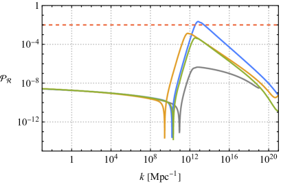
To produce the PBHs with mass in the range $10^{-16}M_{\odot}\lesssim M_{\text{PBH}}\lesssim 10^{-13}M_{\odot}$, in which the PBHs could constitute all the dark matter, the power spectrum should peak at $10^{12}~{}\text{Mpc}^{-1}\lesssim k\lesssim 10^{14}~{}\text{Mpc}^{-1}$. These scales exit the horizon around $30.6\sim 35.2$ e-foldings after the horizon exit of the CMB scales. In our model, the parameter set $P_{1}$ gives $k_{\text{peak}}\simeq 6.7\times 10^{12}~{}\text{Mpc}^{-1}$, leading to the PBHs with $f_{\text{PBH}}\sim 1$ for $M_{\text{PBH}}\simeq 5.6\times 10^{-14}M_{\odot}$.

V The induced gravitational waves

The scalar perturbations decouple with the GWs at linear order. However, they couple at nonlinear orders. Hence, the large scalar perturbations are possible to induce GWs at nonlinear orders. This topic has been widely studied in previous literatures [120, 121, 24, 124, 125, 126, 127]. We follow these works and study the induced GWs in our model. Let us consider the metric

$$\mathrm{d}s^{2}=a^{2}(\tau)\bigg{\{}-\left(1+2\Phi\right)\mathrm{d}\tau^{2}+\bigg{[}(1-2\Psi)\delta_{ij}$$

$$+\frac{1}{2}h_{ij}\bigg{]}\mathrm{d}x^{i}\mathrm{d}x^{j}\bigg{\}},$$ (22)

where $\Phi$ and $\Psi$ are the first order scalar perturbations and $h_{ij}$ is the second order transverse-traceless tensor perturbation, representing the induced GWs. In the absence of anisotropic stress part, one has $\Phi=\Psi$. In Fourier space, the equation of $h_{ij}$ is given by

$$h_{\mathbf{k}}^{\prime\prime}+2\mathcal{H}h_{\mathbf{k}}^{\prime}+k^{2}h_{\mathbf{k}}=4S_{\mathbf{k}},$$ (23)

with $\mathcal{H}=a^{\prime}/a$. Here prime denotes the derivative with respect to the conformal time $\tau$, and $h_{\mathbf{k}}$ is the Fourier mode of $h_{ij}$ defined by

$$h_{ij}(\tau,\mathbf{x})=\int\frac{\mathrm{d}^{3}k}{(2\pi)^{3/2}}e^{i\mathbf{k}\cdot\mathbf{x}}[h_{\mathbf{\mathbf{k}}}(\tau)e_{ij}(\mathbf{k})+\bar{h}_{\mathbf{k}}(\tau)\bar{e}_{ij}(\mathbf{k})],$$ (24)

where $e_{ij}(\mathbf{k})$ and $\bar{e}_{ij}(\mathbf{k})$ are two unit vector bases perpendicular to $\mathbf{k}$ that are orthogonal to each other. $S_{\mathbf{k}}$ is the source term of the induced GWs defined by

$$S_{\mathbf{k}}=\int\frac{\mathrm{d}^{3}q}{(2\pi)^{3/2}}e_{ij}(\mathbf{k})q_{i}q_{j}\Bigg{[}2\Phi_{\mathbf{q}}\Phi_{\mathbf{k}-\mathbf{q}}+\frac{4}{3(1+\omega)}$$

$$\times\left(\frac{\Phi^{\prime}_{\mathbf{q}}}{H}+\Phi_{\mathbf{q}}\right)\left(\frac{\Phi^{\prime}_{\mathbf{k}-\mathbf{q}}}{H}+\Phi_{\mathbf{k}-\mathbf{q}}\right)\Bigg{]}.$$ (25)

Note that the equation of state parameter $\omega$ is introduced.

The energy density of the GWs in sub-horizon is

$$\rho_{GW}=\frac{1}{16a^{2}}\langle\overline{\partial_{k}h_{ij}\partial^{k}h^{ij}}\rangle,$$ (26)

where overline denotes the average over oscillations. The dimensionless power spectrum could be defined by the two-point correlation function,

$$\langle h_{\mathbf{k}}^{\lambda}h_{\mathbf{k^{\prime}}}^{\lambda^{\prime}}\rangle=\delta_{\lambda\lambda^{\prime}}\delta^{3}(\mathbf{k}+\mathbf{k}^{\prime})\frac{2\pi^{3}}{k^{3}}\mathcal{P}_{h}(\tau,k),$$ (27)

where the index $\lambda$, $\lambda^{\prime}$ represent the polarization modes $+$, $\times$. The energy density of GWs per logarithmic wavelength is

$$\Omega_{\mathrm{GW}}=\frac{\rho_{\mathrm{GW}}(\tau,k)}{\rho_{\text{tot}}(k)}=\frac{1}{24}\left(\frac{k}{aH}\right)^{2}\mathcal{P}_{{h}}(\tau,k).$$ (28)

The power spectrum of GWs $\mathcal{P}_{{h}}(\tau,k)$ has a lengthy expression. The final result of the energy density at production is [124]

$$\Omega_{\mathrm{GW,f}}(k)\! \!=\! \!\frac{1}{12}\int_{0}^{\infty}\!\mathrm{d}\upsilon\!\int^{1+\upsilon}_{|1-\upsilon|}\!\mathrm{d}u\!\left(\frac{4\upsilon^{2}-(1+\upsilon^{2}-u^{2})^{2}}{4u\upsilon}\right)^{2}$$ (29)

$$\!\times\! \!\mathcal{P}_{s}(k\upsilon)\mathcal{P}_{s}(ku)\left(\frac{3(u^{2}+\upsilon^{2}-3)}{4u^{3}\upsilon^{3}}\right)^{2}$$

$$\!\times\! \!\!\Bigg{[}\!\left(\!-4u\upsilon+(u^{2}+\upsilon^{2}-3)\log\left|\frac{3-(u+\upsilon)^{2}}{3-(u-\upsilon)^{2}}\right|\right)$$

$$\!+\! \!\pi^{2}(u^{2}+\upsilon^{2}-3)^{2}\Theta(u+\upsilon-\sqrt{3})\Bigg{]},$$

where $\Theta(x)$ is the step function. The energy density of GWs at present time is then

$$\Omega_{\mathrm{GW,0}}=\Omega_{\mathrm{r,0}}\Omega_{\mathrm{GW,f}},$$ (30)

where $\Omega_{\mathrm{r,0}}$ is the energy density of radiation at present time.

Figure 5: The energy density of the induced GWs for parameter sets $P_{1}$ (blue), $P_{2}$ (orange), and $P_{3}$ (green) against the sensitivity curves of future detectors.

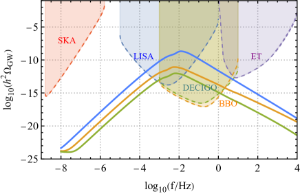
Using the numerical power spectrum, the energy density of the induced GWs can be obtained. The results of our model are shown in Fig. 5. An interesting feature is that, the parameter sets $P_{2}$ and $P_{3}$, which are not expected to produce PBHs, leads to detectable stochastic GWs by future observatories. This is because the induced GWs are not the product of PBHs, but are of the large perturbations. This confirms the idea that the non-detection of stochastic GWs would strongly constrain the early universe. Recently, the pulsar timing array (PTA) collaborations reported strong evidence for the presence of stochastic GW background [129, 130, 131, 132, 133], possibly from supermassive black-hole binaries, but the possibility of other sources like scalar induced GWs are not excluded. If they are induced GWs, it would give a lot of new implications for the primordial curvature perturbations and PBHs [134, 135, 136, 137, 138, 139, 140, 141].

VI Discussion and conclusions

In this work we studied the inflation model proposed in our previous work [82]. The model features a shallow local minimum. Inflation transitions to USR stage when the inflaton rolls over the local minimum. In this stage the perturbations and thus the power spectrum are amplified. For appropriate parameter choices, it is possible to produce PBHs that contribute a large fraction to the dark matter and be consistent with the observations on CMB scales simultaneously. We also studied the induced second order GWs. The GWs are one of the indirect probes of PBHs. The GWs induced by the large perturbations that produce the asteroid mass PBHs are detectable by future experiments like LISA, DECIGO, etc. If these GWs are not observed in future experiments, one would have strong constraints on the primordial scalar power spectrum.

An important issue discussed in this work is the analytical power spectrum. The numerical solution gives the exact power spectrum while the analytical expression would reveal how the power spectrum is controlled by the model parameters. Due to the exponential dependence between the PBH fraction and the power spectrum, a tiny difference of power spectrum would lead to a large deviation of prediction for PBHs. Therefore, an accurate analytical power spectrum would be important and helpful for model building. In this work we give a rough analytical expression. It is accurate for the modes that exit the horizon before the transition to USR but breaks down for the modes exit the horizon in the USR stage. We expect to give a complete and accurate power spectrum in future work.

The coefficients $C_{i}$ and $D_{i}$

For $0\leq N<N_{1}$, the slow-roll conditions are satisfied and we have

$$\mathcal{R}_{k}(N)=CF^{(1)}_{\nu}\left(\frac{k}{aH}\right)+DF^{(2)}_{\nu}\left(\frac{k}{aH}\right),$$ (31)

By imposing the Bunch-Davis initial condition, the coefficients $C_{0}$ and $D_{0}$ can be determined,

$$C_{0}=\frac{iH}{2\sqrt{\epsilon_{1}k^{3}}},\quad D_{0}=-\frac{4H}{3\sqrt{\epsilon_{1}k^{3}}}.$$ (32)

Hence

$$\mathcal{R}^{(0)}_{k}(N)=i\frac{H}{2\sqrt{\epsilon_{*}k^{3}}}e^{i\frac{k}{aH}}\left(1-i\frac{k}{aH}\right).$$ (33)

In the USR stage ($N_{1}\leq N<N_{2}$), the solution is

$$\mathcal{R}^{(1)}_{k}(N)=C_{1}F^{(1)}_{\nu_{u}}\left(\frac{k}{aH}\right)+D_{1}F^{(2)}_{\nu_{u}}\left(\frac{k}{aH}\right),$$ (34)

with $\nu_{u}\simeq(3+\eta_{u})/2$. The coefficients $C_{1}$ and $C_{2}$ are determined by the continuity conditions of $\mathcal{R}_{k}$ and $\mathcal{R}^{\prime}_{k}$ at $N_{1}$, namely,

$$\mathcal{R}^{(0)}_{k}=\mathcal{R}^{(1)}_{k}\big{|}_{N=N_{1}},\quad\mathcal{R^{\prime}}^{(0)}_{k}=\mathcal{R^{\prime}}^{(1)}_{k}\big{|}_{N=N_{1}}.$$ (35)

The result is

$$C_{1}=-\frac{iH}{2\sqrt{k^{3}\epsilon_{*}}}\frac{\frac{k^{2}}{a_{1}^{2}H^{2}}F_{\nu_{u}}^{(2)}\left(\frac{k}{a_{1}H}\right)+\left(1-i\frac{k}{a_{1}H}\right)F_{\nu_{u}}^{\prime(2)}\left(\frac{k}{a_{1}H}\right)}{W\left[F_{\nu_{u}}^{(2)}\left(\frac{k}{a_{1}H}\right),F_{\nu_{u}}^{(1)}\left(\frac{k}{a_{1}H}\right)\right]}e^{i\frac{k}{a_{1}H}},$$ (36)

$$D_{1}=-\frac{iH}{2\sqrt{k^{3}\epsilon_{*}}}\frac{\frac{k^{2}}{a_{1}^{2}H^{2}}F_{\nu_{u}}^{(1)}\left(\frac{k}{a_{1}H}\right)+\left(1-i\frac{k}{a_{1}H}\right)F_{\nu_{u}}^{\prime(1)}\left(\frac{k}{a_{1}H}\right)}{W\left[F_{\nu_{u}}^{(1)}\left(\frac{k}{a_{1}H}\right),F_{\nu_{u}}^{(2)}\left(\frac{k}{a_{1}H}\right)\right]}e^{i\frac{k}{a_{1}H}},$$ (37)

where $\nu_{u}\simeq(3+\eta_{u})/2$ and $W[f,g]=fg^{\prime}-f^{\prime}g$ is the Wronskian. After the USR stage, the inflaton undergoes a constant-roll phase ($N_{2}\leq N\leq N_{3}$), in which the curvature perturbation is

$$\mathcal{R}^{(2)}_{k}(N)=C_{2}F^{(1)}_{\nu_{c}}\left(\frac{k}{aH}\right)+D_{2}F^{(2)}_{\nu_{c}}\left(\frac{k}{aH}\right),$$ (38)

with $\nu_{c}\simeq{3+\eta_{c}}/2$. The coefficients $C_{2}$ and $D_{2}$ can be obtained by repeating the above matching conditions at $N_{2}$,

$$C_{2}=\frac{W\left[C_{1}F^{(1)}_{\nu_{u}}\left(\frac{k}{a_{2}H}\right)+D_{1}F^{(2)}_{\nu_{u}}\left(\frac{k}{a_{2}H}\right),F^{(2)}_{\nu_{c}}\left(\frac{k}{a_{2}H}\right)\right]}{W\left[F_{\nu_{c}}^{(1)}\left(\frac{k}{a_{2}H}\right),F^{(2)}_{\nu_{c}}\left(\frac{k}{a_{2}H}\right)\right]},$$

$$D_{2}=\frac{W\left[C_{1}F^{(1)}_{\nu_{u}}\left(\frac{k}{a_{2}H}\right)+D_{1}F^{(2)}_{\nu_{u}}\left(\frac{k}{a_{2}H}\right),F^{(1)}_{\nu_{c}}\left(\frac{k}{a_{2}H}\right)\right]}{W\left[F_{\nu_{c}}^{(2)}\left(\frac{k}{a_{2}H}\right),F^{(1)}_{\nu_{c}}\left(\frac{k}{a_{2}H}\right)\right]}.$$ (39)

In the final slow-roll stage we have

$$\mathcal{R}^{(3)}_{k}(N)=C_{3}F^{(1)}_{3/2}\left(\frac{k}{aH}\right)+D_{3}F^{(2)}_{3/2}\left(\frac{k}{aH}\right).$$ (40)

Note that we assumed that $\eta=0$ and $\nu=3/2$ in this stage. The coefficients $C_{3}$ and $D_{3}$ are given by the matching at $N_{3}$,

$$C_{3}=\frac{W\left[C_{2}F^{(1)}_{\nu_{c}}\left(\frac{k}{a_{3}H}\right)+D_{2}F^{(2)}_{\nu_{c}}\left(\frac{k}{a_{3}H}\right),F^{(2)}_{3/2}\left(\frac{k}{a_{3}H}\right)\right]}{W\left[F^{(1)}_{3/2}\left(\frac{k}{a_{3}H}\right),F^{(2)}_{3/2}\left(\frac{k}{a_{3}H}\right)\right]},$$

$$D_{3}=\frac{W\left[C_{2}F^{(1)}_{\nu_{c}}\left(\frac{k}{a_{3}H}\right)+D_{2}F^{(2)}_{\nu_{c}}\left(\frac{k}{a_{3}H}\right),F^{(1)}_{3/2}\left(\frac{k}{a_{3}H}\right)\right]}{W\left[F^{(2)}_{3/2}\left(\frac{k}{a_{3}H}\right),F^{(1)}_{3/2}\left(\frac{k}{a_{3}H}\right)\right]}.$$ (41)

Using the asymptotic property of the Bessel functions, we have

$$\lim_{k\ll aH}F^{(1)}_{3/2}\left(\frac{k}{aH}\right)=1,\quad\lim_{k\ll aH}F^{(2)}_{3/2}\left(\frac{k}{aH}\right)=0.$$ (42)

Thus, the power spectrum in the late time limit is given by

$$\mathcal{P}_{\mathcal{R}}(k)=\frac{k^{3}}{2\pi^{2}}\big{|}\mathcal{R}^{(3)}_{k}\big{|}_{k\ll aH}^{2}\simeq\frac{k^{3}}{2\pi^{2}}\big{|}C_{3}\big{|}^{2}.$$ (43)

References

- Akrami et al. [2020] Y. Akrami et al. (Planck), Astron. Astrophys. 641, A10 (2020), arXiv:1807.06211 [astro-ph.CO] .
- Tegmark et al. [2004] M. Tegmark et al. (SDSS), Phys. Rev. D 69, 103501 (2004), arXiv:astro-ph/0310723 .
- Zel’dovich and Novikov [1966] Y. B. Zel’dovich and I. D. Novikov, Sov. Astron. 10, 602 (1966).
- Hawking [1971] S. Hawking, Mon. Not. Roy. Astron. Soc. 152, 75 (1971).
- Carr and Hawking [1974] B. J. Carr and S. W. Hawking, Mon. Not. Roy. Astron. Soc. 168, 399 (1974).
- Sasaki et al. [2016] M. Sasaki, T. Suyama, T. Tanaka, and S. Yokoyama, Phys. Rev. Lett. 117, 061101 (2016), [Erratum: Phys.Rev.Lett. 121, 059901 (2018)], arXiv:1603.08338 [astro-ph.CO] .
- Raidal et al. [2017] M. Raidal, V. Vaskonen, and H. Veermäe, JCAP 09, 037 (2017), arXiv:1707.01480 [astro-ph.CO] .
- Ali-Haïmoud et al. [2017] Y. Ali-Haïmoud, E. D. Kovetz, and M. Kamionkowski, Phys. Rev. D 96, 123523 (2017), arXiv:1709.06576 [astro-ph.CO] .
- Raidal et al. [2019] M. Raidal, C. Spethmann, V. Vaskonen, and H. Veermäe, JCAP 02, 018 (2019), arXiv:1812.01930 [astro-ph.CO] .
- Vaskonen and Veermäe [2020] V. Vaskonen and H. Veermäe, Phys. Rev. D 101, 043015 (2020), arXiv:1908.09752 [astro-ph.CO] .
- De Luca et al. [2020a] V. De Luca, G. Franciolini, P. Pani, and A. Riotto, JCAP 04, 052 (2020a), arXiv:2003.02778 [astro-ph.CO] .
- De Luca et al. [2020b] V. De Luca, G. Franciolini, P. Pani, and A. Riotto, JCAP 06, 044 (2020b), arXiv:2005.05641 [astro-ph.CO] .
- Clesse and Garcia-Bellido [2022] S. Clesse and J. Garcia-Bellido, Phys. Dark Univ. 38, 101111 (2022), arXiv:2007.06481 [astro-ph.CO] .
- Hall et al. [2020] A. Hall, A. D. Gow, and C. T. Byrnes, Phys. Rev. D 102, 123524 (2020), arXiv:2008.13704 [astro-ph.CO] .
- De Luca et al. [2021a] V. De Luca, V. Desjacques, G. Franciolini, P. Pani, and A. Riotto, Phys. Rev. Lett. 126, 051101 (2021a), arXiv:2009.01728 [astro-ph.CO] .
- Wong et al. [2021] K. W. K. Wong, G. Franciolini, V. De Luca, V. Baibhav, E. Berti, P. Pani, and A. Riotto, Phys. Rev. D 103, 023026 (2021), arXiv:2011.01865 [gr-qc] .
- Hütsi et al. [2021] G. Hütsi, M. Raidal, V. Vaskonen, and H. Veermäe, JCAP 03, 068 (2021), arXiv:2012.02786 [astro-ph.CO] .
- De Luca et al. [2021b] V. De Luca, G. Franciolini, P. Pani, and A. Riotto, JCAP 05, 003 (2021b), arXiv:2102.03809 [astro-ph.CO] .
- Franciolini et al. [2022a] G. Franciolini, V. Baibhav, V. De Luca, K. K. Y. Ng, K. W. K. Wong, E. Berti, P. Pani, A. Riotto, and S. Vitale, Phys. Rev. D 105, 083526 (2022a), arXiv:2105.03349 [gr-qc] .
- Franciolini et al. [2022b] G. Franciolini, R. Cotesta, N. Loutrel, E. Berti, P. Pani, and A. Riotto, Phys. Rev. D 105, 063510 (2022b), arXiv:2112.10660 [astro-ph.CO] .
- Franciolini and Pani [2022] G. Franciolini and P. Pani, Phys. Rev. D 105, 123024 (2022), arXiv:2201.13098 [astro-ph.HE] .
- Ivanov et al. [1994] P. Ivanov, P. Naselsky, and I. Novikov, Phys. Rev. D 50, 7173 (1994).
- Carr et al. [2010] B. J. Carr, K. Kohri, Y. Sendouda, and J. Yokoyama, Phys. Rev. D 81, 104019 (2010), arXiv:0912.5297 [astro-ph.CO] .
- Saito and Yokoyama [2010] R. Saito and J. Yokoyama, Prog. Theor. Phys. 123, 867 (2010), [Erratum: Prog.Theor.Phys. 126, 351–352 (2011)], arXiv:0912.5317 [astro-ph.CO] .
- Barnacka et al. [2012] A. Barnacka, J. F. Glicenstein, and R. Moderski, Phys. Rev. D 86, 043001 (2012), arXiv:1204.2056 [astro-ph.CO] .
- Capela et al. [2013] F. Capela, M. Pshirkov, and P. Tinyakov, Phys. Rev. D 87, 123524 (2013), arXiv:1301.4984 [astro-ph.CO] .
- Carr et al. [2016] B. Carr, F. Kuhnel, and M. Sandstad, Phys. Rev. D 94, 083504 (2016), arXiv:1607.06077 [astro-ph.CO] .
- Niikura et al. [2019a] H. Niikura et al., Nature Astron. 3, 524 (2019a), arXiv:1701.02151 [astro-ph.CO] .
- Carr et al. [2017] B. Carr, M. Raidal, T. Tenkanen, V. Vaskonen, and H. Veermäe, Phys. Rev. D 96, 023514 (2017), arXiv:1705.05567 [astro-ph.CO] .
- Zumalacarregui and Seljak [2018] M. Zumalacarregui and U. Seljak, Phys. Rev. Lett. 121, 141101 (2018), arXiv:1712.02240 [astro-ph.CO] .
- Sasaki et al. [2018] M. Sasaki, T. Suyama, T. Tanaka, and S. Yokoyama, Class. Quant. Grav. 35, 063001 (2018), arXiv:1801.05235 [astro-ph.CO] .
- Niikura et al. [2019b] H. Niikura, M. Takada, S. Yokoyama, T. Sumi, and S. Masaki, Phys. Rev. D 99, 083503 (2019b), arXiv:1901.07120 [astro-ph.CO] .
- Montero-Camacho et al. [2019] P. Montero-Camacho, X. Fang, G. Vasquez, M. Silva, and C. M. Hirata, JCAP 08, 031 (2019), arXiv:1906.05950 [astro-ph.CO] .
- Laha [2019] R. Laha, Phys. Rev. Lett. 123, 251101 (2019), arXiv:1906.09994 [astro-ph.HE] .
- Dasgupta et al. [2020] B. Dasgupta, R. Laha, and A. Ray, Phys. Rev. Lett. 125, 101101 (2020), arXiv:1912.01014 [hep-ph] .
- Carr et al. [2021] B. Carr, K. Kohri, Y. Sendouda, and J. Yokoyama, Rept. Prog. Phys. 84, 116902 (2021), arXiv:2002.12778 [astro-ph.CO] .
- Carr and Kuhnel [2020] B. Carr and F. Kuhnel, Ann. Rev. Nucl. Part. Sci. 70, 355 (2020), arXiv:2006.02838 [astro-ph.CO] .
- Green and Kavanagh [2021] A. M. Green and B. J. Kavanagh, J. Phys. G 48, 043001 (2021), arXiv:2007.10722 [astro-ph.CO] .
- Mittal et al. [2022] S. Mittal, A. Ray, G. Kulkarni, and B. Dasgupta, JCAP 03, 030 (2022), arXiv:2107.02190 [astro-ph.CO] .
- Özsoy and Tasinato [2023] O. Özsoy and G. Tasinato, (2023), arXiv:2301.03600 [astro-ph.CO] .
- Fixsen et al. [1996] D. J. Fixsen, E. S. Cheng, J. M. Gales, J. C. Mather, R. A. Shafer, and E. L. Wright, Astrophys. J. 473, 576 (1996), arXiv:astro-ph/9605054 .
- Chluba et al. [2012] J. Chluba, A. L. Erickcek, and I. Ben-Dayan, Astrophys. J. 758, 76 (2012), arXiv:1203.2681 [astro-ph.CO] .
- Kohri et al. [2014] K. Kohri, T. Nakama, and T. Suyama, Phys. Rev. D 90, 083514 (2014), arXiv:1405.5999 [astro-ph.CO] .
- Nakama et al. [2018] T. Nakama, B. Carr, and J. Silk, Phys. Rev. D 97, 043525 (2018), arXiv:1710.06945 [astro-ph.CO] .
- Diego et al. [2018] J. M. Diego et al., Astrophys. J. 857, 25 (2018), arXiv:1706.10281 [astro-ph.CO] .
- Oguri et al. [2018] M. Oguri, J. M. Diego, N. Kaiser, P. L. Kelly, and T. Broadhurst, Phys. Rev. D 97, 023518 (2018), arXiv:1710.00148 [astro-ph.CO] .
- Chen et al. [2020a] Z.-C. Chen, C. Yuan, and Q.-G. Huang, Phys. Rev. Lett. 124, 251101 (2020a), arXiv:1910.12239 [astro-ph.CO] .
- Young et al. [2014] S. Young, C. T. Byrnes, and M. Sasaki, JCAP 07, 045 (2014), arXiv:1405.7023 [gr-qc] .
- Young and Byrnes [2013] S. Young and C. T. Byrnes, JCAP 08, 052 (2013), arXiv:1307.4995 [astro-ph.CO] .
- Pattison et al. [2017] C. Pattison, V. Vennin, H. Assadullahi, and D. Wands, JCAP 10, 046 (2017), arXiv:1707.00537 [hep-th] .
- Franciolini et al. [2018] G. Franciolini, A. Kehagias, S. Matarrese, and A. Riotto, JCAP 03, 016 (2018), arXiv:1801.09415 [astro-ph.CO] .
- Biagetti et al. [2018] M. Biagetti, G. Franciolini, A. Kehagias, and A. Riotto, JCAP 07, 032 (2018), arXiv:1804.07124 [astro-ph.CO] .
- Ezquiaga and García-Bellido [2018] J. M. Ezquiaga and J. García-Bellido, JCAP 08, 018 (2018), arXiv:1805.06731 [astro-ph.CO] .
- Atal and Germani [2019] V. Atal and C. Germani, Phys. Dark Univ. 24, 100275 (2019), arXiv:1811.07857 [astro-ph.CO] .
- Passaglia et al. [2019] S. Passaglia, W. Hu, and H. Motohashi, Phys. Rev. D 99, 043536 (2019), arXiv:1812.08243 [astro-ph.CO] .
- Young et al. [2019] S. Young, I. Musco, and C. T. Byrnes, JCAP 11, 012 (2019), arXiv:1904.00984 [astro-ph.CO] .
- Young [2019] S. Young, Int. J. Mod. Phys. D 29, 2030002 (2019), arXiv:1905.01230 [astro-ph.CO] .
- Kehagias et al. [2019] A. Kehagias, I. Musco, and A. Riotto, JCAP 12, 029 (2019), arXiv:1906.07135 [astro-ph.CO] .
- Ezquiaga et al. [2020] J. M. Ezquiaga, J. García-Bellido, and V. Vennin, JCAP 03, 029 (2020), arXiv:1912.05399 [astro-ph.CO] .
- Kitajima et al. [2021] N. Kitajima, Y. Tada, S. Yokoyama, and C.-M. Yoo, JCAP 10, 053 (2021), arXiv:2109.00791 [astro-ph.CO] .
- Figueroa et al. [2022] D. G. Figueroa, S. Raatikainen, S. Rasanen, and E. Tomberg, JCAP 05, 027 (2022), arXiv:2111.07437 [astro-ph.CO] .
- Cai et al. [2021a] Y.-F. Cai, X.-H. Ma, M. Sasaki, D.-G. Wang, and Z. Zhou, (2021a), arXiv:2112.13836 [astro-ph.CO] .
- Cai et al. [2022] Y.-F. Cai, X.-H. Ma, M. Sasaki, D.-G. Wang, and Z. Zhou, JCAP 12, 034 (2022), arXiv:2207.11910 [astro-ph.CO] .
- Young [2022] S. Young, JCAP 05, 037 (2022), arXiv:2201.13345 [astro-ph.CO] .
- Ferrante et al. [2023] G. Ferrante, G. Franciolini, A. Iovino, Junior., and A. Urbano, Phys. Rev. D 107, 043520 (2023), arXiv:2211.01728 [astro-ph.CO] .
- Pi and Sasaki [2023] S. Pi and M. Sasaki, Phys. Rev. Lett. 131, 011002 (2023), arXiv:2211.13932 [astro-ph.CO] .
- van Laak and Young [2023] R. van Laak and S. Young, JCAP 05, 058 (2023), arXiv:2303.05248 [astro-ph.CO] .
- Yokoyama [1998] J. Yokoyama, Phys. Rev. D 58, 083510 (1998), arXiv:astro-ph/9802357 .
- Cheng et al. [2017] S.-L. Cheng, W. Lee, and K.-W. Ng, JHEP 02, 008 (2017), arXiv:1606.00206 [astro-ph.CO] .
- Garcia-Bellido and Ruiz Morales [2017] J. Garcia-Bellido and E. Ruiz Morales, Phys. Dark Univ. 18, 47 (2017), arXiv:1702.03901 [astro-ph.CO] .
- Ezquiaga et al. [2018] J. M. Ezquiaga, J. Garcia-Bellido, and E. Ruiz Morales, Phys. Lett. B 776, 345 (2018), arXiv:1705.04861 [astro-ph.CO] .
- Germani and Prokopec [2017] C. Germani and T. Prokopec, Phys. Dark Univ. 18, 6 (2017), arXiv:1706.04226 [astro-ph.CO] .
- Cicoli et al. [2018] M. Cicoli, V. A. Diaz, and F. G. Pedro, JCAP 06, 034 (2018), arXiv:1803.02837 [hep-th] .
- Özsoy et al. [2018] O. Özsoy, S. Parameswaran, G. Tasinato, and I. Zavala, JCAP 07, 005 (2018), arXiv:1803.07626 [hep-th] .
- Cicoli et al. [2022] M. Cicoli, F. G. Pedro, and N. Pedron, JCAP 08, 030 (2022), arXiv:2203.00021 [hep-th] .
- Kannike et al. [2017] K. Kannike, L. Marzola, M. Raidal, and H. Veermäe, JCAP 09, 020 (2017), arXiv:1705.06225 [astro-ph.CO] .
- Ballesteros and Taoso [2018] G. Ballesteros and M. Taoso, Phys. Rev. D 97, 023501 (2018), arXiv:1709.05565 [hep-ph] .
- Hertzberg and Yamada [2018] M. P. Hertzberg and M. Yamada, Phys. Rev. D 97, 083509 (2018), arXiv:1712.09750 [astro-ph.CO] .
- Mishra and Sahni [2020] S. S. Mishra and V. Sahni, JCAP 04, 007 (2020), arXiv:1911.00057 [gr-qc] .
- Figueroa et al. [2021] D. G. Figueroa, S. Raatikainen, S. Rasanen, and E. Tomberg, Phys. Rev. Lett. 127, 101302 (2021), arXiv:2012.06551 [astro-ph.CO] .
- Karam et al. [2022] A. Karam, N. Koivunen, E. Tomberg, V. Vaskonen, and H. Veermäe, (2022), arXiv:2205.13540 [astro-ph.CO] .
- Gu et al. [2023] B.-M. Gu, F.-W. Shu, K. Yang, and Y.-P. Zhang, Phys. Rev. D 107, 023519 (2023), arXiv:2207.09968 [astro-ph.CO] .
- Kefala et al. [2021] K. Kefala, G. P. Kodaxis, I. D. Stamou, and N. Tetradis, Phys. Rev. D 104, 023506 (2021), arXiv:2010.12483 [astro-ph.CO] .
- Inomata et al. [2021] K. Inomata, E. McDonough, and W. Hu, Phys. Rev. D 104, 123553 (2021), arXiv:2104.03972 [astro-ph.CO] .
- Dalianis et al. [2021] I. Dalianis, G. P. Kodaxis, I. D. Stamou, N. Tetradis, and A. Tsigkas-Kouvelis, Phys. Rev. D 104, 103510 (2021), arXiv:2106.02467 [astro-ph.CO] .
- Inomata et al. [2022] K. Inomata, E. McDonough, and W. Hu, JCAP 02, 031 (2022), arXiv:2110.14641 [astro-ph.CO] .
- Kristiano and Yokoyama [2022] J. Kristiano and J. Yokoyama, (2022), arXiv:2211.03395 [hep-th] .
- Riotto [2023] A. Riotto, (2023), arXiv:2301.00599 [astro-ph.CO] .
- Choudhury et al. [2023a] S. Choudhury, M. R. Gangopadhyay, and M. Sami, (2023a), arXiv:2301.10000 [astro-ph.CO] .
- Choudhury et al. [2023b] S. Choudhury, S. Panda, and M. Sami, (2023b), arXiv:2302.05655 [astro-ph.CO] .
- Kristiano and Yokoyama [2023] J. Kristiano and J. Yokoyama, (2023), arXiv:2303.00341 [hep-th] .
- Choudhury et al. [2023c] S. Choudhury, S. Panda, and M. Sami, (2023c), arXiv:2303.06066 [astro-ph.CO] .
- Firouzjahi and Riotto [2023] H. Firouzjahi and A. Riotto, (2023), arXiv:2304.07801 [astro-ph.CO] .
- Franciolini et al. [2023a] G. Franciolini, A. Iovino, Junior., M. Taoso, and A. Urbano, (2023a), arXiv:2305.03491 [astro-ph.CO] .
- Fumagalli [2023] J. Fumagalli, (2023), arXiv:2305.19263 [astro-ph.CO] .
- Cai et al. [2018] Y.-F. Cai, X. Tong, D.-G. Wang, and S.-F. Yan, Phys. Rev. Lett. 121, 081306 (2018), arXiv:1805.03639 [astro-ph.CO] .
- Ballesteros et al. [2019] G. Ballesteros, J. Beltran Jimenez, and M. Pieroni, JCAP 06, 016 (2019), arXiv:1811.03065 [astro-ph.CO] .
- Kamenshchik et al. [2019] A. Y. Kamenshchik, A. Tronconi, T. Vardanyan, and G. Venturi, Phys. Lett. B 791, 201 (2019), arXiv:1812.02547 [gr-qc] .
- Lin et al. [2020] J. Lin, Q. Gao, Y. Gong, Y. Lu, C. Zhang, and F. Zhang, Phys. Rev. D 101, 103515 (2020), arXiv:2001.05909 [gr-qc] .
- Chen et al. [2020b] C. Chen, X.-H. Ma, and Y.-F. Cai, Phys. Rev. D 102, 063526 (2020b), arXiv:2003.03821 [astro-ph.CO] .
- Yi et al. [2021] Z. Yi, Q. Gao, Y. Gong, and Z.-h. Zhu, Phys. Rev. D 103, 063534 (2021), arXiv:2011.10606 [astro-ph.CO] .
- Solbi and Karami [2021] M. Solbi and K. Karami, JCAP 08, 056 (2021), arXiv:2102.05651 [astro-ph.CO] .
- Teimoori et al. [2021] Z. Teimoori, K. Rezazadeh, M. A. Rasheed, and K. Karami, (2021), arXiv:2107.07620 [astro-ph.CO] .
- Pi et al. [2018] S. Pi, Y.-l. Zhang, Q.-G. Huang, and M. Sasaki, JCAP 05, 042 (2018), arXiv:1712.09896 [astro-ph.CO] .
- Fu et al. [2019] C. Fu, P. Wu, and H. Yu, Phys. Rev. D 100, 063532 (2019), arXiv:1907.05042 [astro-ph.CO] .
- Heydari and Karami [2022] S. Heydari and K. Karami, Eur. Phys. J. C 82, 83 (2022), arXiv:2107.10550 [gr-qc] .
- Kawai and Kim [2021] S. Kawai and J. Kim, Phys. Rev. D 104, 083545 (2021), arXiv:2108.01340 [astro-ph.CO] .
- Frolovsky et al. [2022] D. Frolovsky, S. V. Ketov, and S. Saburov, Mod. Phys. Lett. A 37, 2250135 (2022), arXiv:2205.00603 [astro-ph.CO] .
- Garcia-Bellido et al. [1996] J. Garcia-Bellido, A. D. Linde, and D. Wands, Phys. Rev. D 54, 6040 (1996), arXiv:astro-ph/9605094 .
- Palma et al. [2020] G. A. Palma, S. Sypsas, and C. Zenteno, Phys. Rev. Lett. 125, 121301 (2020), arXiv:2004.06106 [astro-ph.CO] .
- Braglia et al. [2020] M. Braglia, D. K. Hazra, F. Finelli, G. F. Smoot, L. Sriramkumar, and A. A. Starobinsky, JCAP 08, 001 (2020), arXiv:2005.02895 [astro-ph.CO] .
- Cai et al. [2021b] R.-G. Cai, C. Chen, and C. Fu, Phys. Rev. D 104, 083537 (2021b), arXiv:2108.03422 [astro-ph.CO] .
- Hooshangi et al. [2022] S. Hooshangi, A. Talebian, M. H. Namjoo, and H. Firouzjahi, Phys. Rev. D 105, 083525 (2022), arXiv:2201.07258 [astro-ph.CO] .
- Geller et al. [2022] S. R. Geller, W. Qin, E. McDonough, and D. I. Kaiser, Phys. Rev. D 106, 063535 (2022), arXiv:2205.04471 [hep-th] .
- Chongchitnan and Efstathiou [2007] S. Chongchitnan and G. Efstathiou, JCAP 01, 011 (2007), arXiv:astro-ph/0611818 .
- Motohashi and Hu [2017] H. Motohashi and W. Hu, Phys. Rev. D 96, 063503 (2017), arXiv:1706.06784 [astro-ph.CO] .
- Byrnes et al. [2019] C. T. Byrnes, P. S. Cole, and S. P. Patil, JCAP 06, 028 (2019), arXiv:1811.11158 [astro-ph.CO] .
- Liu et al. [2020] J. Liu, Z.-K. Guo, and R.-G. Cai, Phys. Rev. D 101, 083535 (2020), arXiv:2003.02075 [astro-ph.CO] .
- Tasinato [2021] G. Tasinato, Phys. Rev. D 103, 023535 (2021), arXiv:2012.02518 [hep-th] .
- Ananda et al. [2007] K. N. Ananda, C. Clarkson, and D. Wands, Phys. Rev. D 75, 123518 (2007), arXiv:gr-qc/0612130 .
- [121] D. Baumann, K. Ichiki, P. J. Steinhardt, and K. Takahashi, 10.1103/PhysRevD.76.084019, hep-th/0703290v1 .
- Saito and Yokoyama [2009] R. Saito and J. Yokoyama, Phys. Rev. Lett. 102, 161101 (2009), [Erratum: Phys.Rev.Lett. 107, 069901 (2011)], arXiv:0812.4339 [astro-ph] .
- Bugaev and Klimai [2010] E. Bugaev and P. Klimai, Phys. Rev. D 81, 023517 (2010), arXiv:0908.0664 [astro-ph.CO] .
- Kohri and Terada [2018] K. Kohri and T. Terada, Phys. Rev. D 97, 123532 (2018), arXiv:1804.08577 [gr-qc] .
- Cai et al. [2019] R.-g. Cai, S. Pi, and M. Sasaki, Phys. Rev. Lett. 122, 201101 (2019), arXiv:1810.11000 [astro-ph.CO] .
- Inomata and Nakama [2019] K. Inomata and T. Nakama, Phys. Rev. D 99, 043511 (2019), arXiv:1812.00674 [astro-ph.CO] .
- Domènech [2021] G. Domènech, Universe 7, 398 (2021), arXiv:2109.01398 [gr-qc] .
- Cole et al. [2022] P. S. Cole, A. D. Gow, C. T. Byrnes, and S. P. Patil, (2022), arXiv:2204.07573 [astro-ph.CO] .
- Xu et al. [2023] H. Xu et al., Res. Astron. Astrophys. 23, 075024 (2023), arXiv:2306.16216 [astro-ph.HE] .
- Agazie et al. [2023a] G. Agazie et al. (NANOGrav), Astrophys. J. Lett. 951, L8 (2023a), arXiv:2306.16213 [astro-ph.HE] .
- Agazie et al. [2023b] G. Agazie et al. (NANOGrav), Astrophys. J. Lett. 951, L9 (2023b), arXiv:2306.16217 [astro-ph.HE] .
- Reardon et al. [2023] D. J. Reardon et al., Astrophys. J. Lett. 951, L6 (2023), arXiv:2306.16215 [astro-ph.HE] .
- Antoniadis et al. [2023] J. Antoniadis et al., (2023), arXiv:2306.16214 [astro-ph.HE] .
- Arzoumanian et al. [2018] Z. Arzoumanian et al. (NANOGRAV), Astrophys. J. 859, 47 (2018), arXiv:1801.02617 [astro-ph.HE] .
- Ashoorioon et al. [2022] A. Ashoorioon, K. Rezazadeh, and A. Rostami, Phys. Lett. B 835, 137542 (2022), arXiv:2202.01131 [astro-ph.CO] .
- Cai et al. [2023] Y.-F. Cai, X.-C. He, X. Ma, S.-F. Yan, and G.-W. Yuan, (2023), arXiv:2306.17822 [gr-qc] .
- Inomata et al. [2023] K. Inomata, K. Kohri, and T. Terada, (2023), arXiv:2306.17834 [astro-ph.CO] .
- Depta et al. [2023] P. F. Depta, K. Schmidt-Hoberg, and C. Tasillo, (2023), arXiv:2306.17836 [astro-ph.CO] .
- Franciolini et al. [2023b] G. Franciolini, A. Iovino, Junior., V. Vaskonen, and H. Veermae, (2023b), arXiv:2306.17149 [astro-ph.CO] .
- Liu et al. [2023] L. Liu, Z.-C. Chen, and Q.-G. Huang, (2023), arXiv:2307.01102 [astro-ph.CO] .
- Firouzjahi and Talebian [2023] H. Firouzjahi and A. Talebian, (2023), arXiv:2307.03164 [gr-qc] .