A nontopological soliton in an $\mathcal{N}=1$ supersymmetric gauge Abelian model

Abstract

A version of $\mathcal{N}=1$ supersymmetric scalar electrodynamics is considered here, and it is shown that an electrically charged nontopological soliton exists in this model. In addition to the long-range electric field, the soliton also possesses a long-range scalar field, which leads to a modification of the intersoliton interaction potential at large distances. The supersymmetry of the model makes it possible to express fermionic zero modes of the soliton in terms of bosonic fields. The properties of the nontopological soliton are investigated using analytical and numerical methods.

1 Introduction

Many models of field theory have solutions that describe spatially localised and nonspreading field configurations with a finite energy [1, 2]. Nontopological solitons [3] represent one of these field configurations. A necessary condition for the existence of a nontopological soliton is the symmetry of the corresponding field model, which may be both global and local. In addition, the interaction potentials of the model must meet a certain condition [4, 5]. The symmetry of the model results in the existence of a conserved Noether charge. The field configuration of a nontopological soliton is an extremum (minimum or saddle point) of the energy functional at a fixed value of the Noether charge, and this basic property largely determines the other properties of a nontopological soliton; in particular, it leads to the characteristic time dependence $\exp\left(-i\omega t\right)$ of a soliton field.

Nontopological solitons may be formed during a primordial phase transition, thus making a contribution to various scenarios of the evolution of the early Universe [6]. Furthermore, they may play an essential role in baryogenesis via the Affleck-Dine mechanism [7], and are considered to be places where dark matter may be concentrated [8].

Some field models with local Abelian symmetry admit the existence of electrically charged nontopological solitons. First described in Refs. [9, 10], they have since been investigated in many other works (see, e.g., Refs. [11, 12, 13, 14, 15, 16, 17, 18, 19, 20, 21, 22, 23]). The properties of electrically charged solitons differ significantly from those of solitons without an electric charge; in particular, the electric charge and the energy of a nontopological soliton cannot be arbitrarily large in the general case [10, 20]. In addition, an electrically charged nontopological soliton can exist only if the gauge coupling constant does not exceed some maximum value [10].

The main goal of this work is to study a non-topological soliton in a version of $\mathcal{N}=1$ supersymmetric scalar electrodynamics. The interaction potential of this model is expressed in terms of a superpotential, which leads to relations between the nonlinear interaction constants. In addition, the superpotential largely determines the form of the scalar-fermion interaction. The requirements of renormalisability and gauge invariance impose severe restrictions on the form of the superpotential, all of which significantly reduces the number of model parameters compared to the nonsupersymmetric case.

Throughout this paper, we use the natural units $c=1$, $\hbar=1$. The metric tensor and the Dirac matrices are defined according to Ref. [24].

2 Lagrangian and field equations of the model

The $\mathcal{N}=1$ supersymmetric gauge model under consideration includes three left-chiral matter superfields $\Phi_{-1}$, $\Phi_{0}$, and $\Phi_{+1}$, and one Abelian gauge superfield $V$. The left-chiral superfield $\Phi_{n}$ contains two components: the complex scalar field $\phi_{n}$ and the left-hand Dirac spinor field $\psi_{nL}$. Written in the Wess-Zumino gauge, the gauge superfield $V$ also contains two components: the Abelian gauge field $A_{\mu}$ and the Majorana spinor field $\lambda$. The superfields $\Phi_{n}$ and $V$ also contain auxiliary fields, but these can be expressed in terms of the above mentioned physical fields.

The Lagrangian of the model takes the form

$$\mathcal{L}=-\frac{1}{4}F_{\mu\nu}F^{\mu\nu}-\sum\limits_{n}\left(D_{\mu}\phi_{n}\right)^{\ast}D^{\mu}\phi_{n}-V\left(\phi\right)$$

$$-\frac{1}{2}\bar{\lambda}\gamma^{\mu}\partial_{\mu}\lambda-\sum\limits_{n}\overline{\psi_{nL}}\gamma^{\mu}D_{\mu}\psi_{nL}$$

$$-\frac{1}{2}\sum\limits_{nm}\left\{f_{nm}\left(\psi_{nL}^{\text{T}}\epsilon\psi_{mL}\right)+f_{nm}^{\ast}\left(\psi_{nL}^{\text{T}}\epsilon\psi_{mL}\right)^{\ast}\right\}$$

$$+i\sqrt{2}\sum\limits_{n}q_{n}\left\{\phi_{n}\left(\overline{\psi_{nL}}\lambda\right)-\phi_{n}^{\ast}\left(\bar{\lambda}\psi_{nL}\right)\right\}.$$ (1)

In Eq. (1), the matrix $\epsilon=-i\gamma_{0}\gamma_{2}\gamma_{5}$, the Latin indices $n$ and $m$ run over the set $[-1,0,1]$, and the covariant derivatives

$$D_{\mu}\phi_{n} =\partial_{\mu}\phi_{n}-iq_{n}A_{\mu}\phi_{n},$$ (2a)

$$D_{\mu}\psi_{n} =\partial_{\mu}\psi_{n}-iq_{n}A_{\mu}\psi_{n},$$ (2b)

where $q_{n}=ne$ are the Abelian charges of the left-chiral superfield $\Phi_{n}$. To avoid $U(1)$-$U(1)$-$U(1)$ and $U(1)$-graviton-graviton anomalies, the sum of the $U(1)$ quantum numbers of all left-chiral superfields and the sum of their cubes should vanish, which is obviously true in our case. The field-dependent coefficients $f_{nm}$ and the interaction potential $V\left(\phi\right)$ are expressed in terms of the superpotential

$$f\left(\phi\right)=m\phi_{-1}\phi_{+1}+g\phi_{-1}\phi_{0}\phi_{+1},$$ (3)

where $m$ is a mass parameter and $g$ is a coupling constant. The coefficients $f_{nm}=\partial^{2}f/\partial\phi_{n}\partial\phi_{m}$, and the interaction potential

$$V\left(\phi\right) =\sum\limits_{n}\left|\partial f/\partial\phi_{n}\right|^{2}+\frac{1}{2}\Bigl{(}\sum\limits_{n}q_{n}\phi_{n}^{\ast}\phi_{n}\Bigr{)}^{2}$$

$$=\left|m+g\phi_{0}\right|^{2}\left(\left|\phi_{-1}\right|^{2}+\left|\phi_{+1}\right|^{2}\right)$$

$$+g^{2}\left|\phi_{-1}\right|^{2}\left|\phi_{+1}\right|^{2}$$

$$+\frac{e^{2}}{2}\left(\left|\phi_{+1}\right|^{2}-\left|\phi_{-1}\right|^{2}\right)^{2}.$$ (4)

The field equations of model (1) have the form

$$\partial_{\mu}F^{\mu\nu}=j^{\nu},$$ (5)

$$D_{\mu}D^{\mu}\phi_{n}-\frac{\partial V}{\partial\phi_{n}^{\ast}}-\frac{1}{2}\sum\limits_{k^{\prime}m^{\prime}}f_{k^{\prime}m^{\prime}n}^{\ast}\left(\psi_{k^{\prime}L}^{\text{T}}\epsilon\psi_{m^{\prime}L}\right)^{\ast}$$

$$-i\sqrt{2}q_{n}\left(\overline{\lambda}\psi_{nL}\right)=0,$$ (6)

$$\not{D}\psi_{nL}-\sum\limits_{m^{\prime}}f_{nm^{\prime}}^{\ast}\epsilon\left(\overline{\psi_{m^{\prime}L}}\right)^{\text{T}}-i\sqrt{2}q_{n}\phi_{n}\lambda_{R}=0,$$ (7)

$$\not{\partial}\lambda+i\sqrt{2}\sum\limits_{m^{\prime}}q_{m^{\prime}}\left\{\phi_{m^{\prime}}\epsilon\left(\overline{\psi_{m^{\prime}L}}\right)^{\text{T}}+\phi_{m^{\prime}}^{\ast}\psi_{m^{\prime}L}\right\}=0,$$ (8)

where the coefficients $f_{kmn}=\partial^{3}f/\partial\phi_{k}\partial\phi_{m}\partial\phi_{n}$ and the electromagnetic current

$$j^{\nu}=i\sum\limits_{n}q_{n}\phi_{n}^{\ast}\overset{\longleftrightarrow}{D^{\nu}}\phi_{n}-i\sum\limits_{n}q_{n}\overline{\psi_{nL}}\gamma^{\nu}\psi_{nL}.$$ (9)

Later on, we shall also need the expression for the energy density of an electrically charged bosonic field configuration of the model

$$\mathcal{E} =\frac{1}{2}E_{i}E_{i}+\sum\limits_{n}\left\{\left(D_{t}\phi_{n}\right)^{\ast}D_{t}\phi_{n}\right.$$

$$\left.+\left(D_{i}\phi_{n}\right)^{\ast}D_{i}\phi_{n}\right\}+V\left(\phi\right),$$ (10)

where $E_{i}=F_{i0}$ are the components of the electric field strength.

3 Ansatz and some properties of the nontopological soliton

The model (1) can be viewed as the Abelian gauge version of a model of the Wess-Zumino type [25]. In Ref. [26], it was shown that for superpotentials of the type in Eq. (3), these models admit the existence of nontopological solitons. It follows from continuity considerations that nontopological solitons can also exist in gauge model (1), at least for sufficiently small values of the gauge coupling constant $e$.

Let us define the shifted field $\varphi_{0}\left(\mathbf{x},t\right)=mg^{-1}+\phi_{0}\left(\mathbf{x},t\right)$. To find a nontopological soliton solution, we shall use the spherically symmetrical ansatz:

$$\phi_{+1}\left(\mathbf{x},t\right) =2^{-\frac{1}{2}}\exp\left(-i\omega t\right)f_{+1}\left(r\right),$$ (11a)

$$\phi_{-1}\left(\mathbf{x},t\right) =2^{-\frac{1}{2}}\exp\left(i\omega t\right)f_{-1}\left(r\right),$$ (11b)

$$\varphi_{0}\left(\mathbf{x},t\right) =2^{-\frac{1}{2}}(\chi_{1}\left(r\right)+i\chi_{2}\left(r\right)),$$ (11c)

$$A^{\mu}\left(\mathbf{x},t\right) =\left(\Phi\left(r\right),\,0\right).$$ (11d)

The energy density (10), written in terms of the ansatz functions (11), takes the form

$$\mathcal{E} =\frac{1}{2}\Omega^{2}\left(f_{-1}^{2}+f_{+1}^{2}\right)+\frac{1}{2}\Phi^{\prime 2}$$

$$+\frac{1}{2}\left(f_{-1}^{\prime 2}+f_{+1}^{\prime 2}+\chi_{1}^{\prime 2}+\chi_{2}^{\prime 2}\right)+V,$$ (12)

where the interaction potential

$$V =\frac{g^{2}}{4}\left(f_{-1}^{2}+f_{+1}^{2}\right)\left(\chi_{1}^{2}+\chi_{2}^{2}\right)$$

$$+\frac{g^{2}}{4}f_{-1}^{2}f_{+1}^{2}+\frac{e^{2}}{8}\left(f_{+1}^{2}-f_{-1}^{2}\right)^{2},$$ (13)

the function $\Omega\left(r\right)=\omega-e\Phi\left(r\right)$, and the prime indicates the derivative with respect to $r$. The Lagrangian density $\mathcal{L}$ differs from the energy density $\mathcal{E}$ only in regard to the sign of the terms in the second line of Eq. (12). The electromagnetic current of spherically symmetrical field configuration (11) is

$$j^{\nu}=\left(e\Omega\left(f_{-1}^{2}+f_{+1}^{2}\right),0,0,0\right).$$ (14)

Substituting ansatz (11) into the bosonic parts of field equations (5) and (6), we obtain a system of nonlinear differential equations for the ansatz functions:

$$\Omega^{\prime\prime}+\frac{2}{r}\Omega^{\prime}-e^{2}\left(f_{-1}^{2}+f_{+1}^{2}\right)\Omega=0,$$ (15)

$$f_{\pm 1}^{\prime\prime}+\frac{2}{r}f_{\pm 1}^{\prime}+\frac{\partial U}{\partial f_{\pm 1}}=0,$$ (16)

$$\chi_{1,2}^{\prime\prime}+\frac{2}{r}\chi_{1,2}^{\prime}+\frac{\partial U}{\partial\chi_{1,2}}=0,$$ (17)

where the effective potential

$$U=\frac{1}{2}\Omega^{2}\left(f_{-1}^{2}+f_{+1}^{2}\right)-V.$$ (18)

The regularity of the soliton field configuration and the finiteness of the soliton energy lead to the following boundary conditions:

$$f_{\pm 1}^{\prime}\left(0\right) =0, f_{\pm 1}\left(r\right) \underset{r\rightarrow\infty}{\longrightarrow}0,$$ (19a)

$$\chi_{1,2}^{\prime}\left(0\right) =0, \chi_{1,2}\left(r\right) \underset{r\rightarrow\infty}{\longrightarrow}\chi_{1,2\,\text{vac}},$$ (19b)

$$\Omega^{\prime}\left(0\right) =0, \Omega\left(r\right) \underset{r\rightarrow\infty}{\longrightarrow}\omega.$$ (19c)

The boundary conditions in Eqs. (19b) and (19c) need some explanation. From Eqs. (1) and (4), it follows that the classical vacuum of model (1) is

$$F_{\mu\nu}=0,\quad\phi_{\pm 1}=0,\quad\phi_{0}=\phi_{0\,\text{vac}},$$ (20)

where $\phi_{0\,\text{vac}}$ is an arbitrary complex constant. From Eq. (20), it follows that model (1) has an infinite number of vacua at the classical level, as reflected in the boundary condition in Eq. (19b). All of these vacua are invariant under both the $U(1)$ gauge and $\mathcal{N}=1$ supersymmetry transformations. According to the non-renormalisation theorems [27, 28], this will also be true when perturbative quantum corrections are taken into account.

Eqs. (13), (17), and (18) tell us that $\chi_{1}$ and $\chi_{2}$ satisfy the same linear homogeneous differential equation, while Eq. (19b) tells us that $\chi_{1}$ and $\chi_{2}$ satisfy the same homogeneous boundary condition at $r=0$. It follows that the ratio $\chi_{2}(r)/\chi_{1}(r)$ does not depend on $r$, and is equal to $\chi_{2\,\text{vac}}/\chi_{1\,\text{vac}}$. The phase of the ansatz function $\varphi_{0}(r)=2^{-1/2}(\chi_{1}(r)+i\chi_{2}(r))$ is therefore a constant. However, from Eqs. (12) and (13), it follows that in this case, the energy density and the Lagrangian density do not depend on the phase of $\varphi_{0}\left(r\right)$. Without loss of generality, we can set this phase (and hence $\chi_{2}(r)$) equal to zero.

The field configurations of model (1) are determined up to gauge transformations. In particular, the choice of ansatz (11) is equivalent to the choice of the radial gauge. However, this gauge does not fix the soliton field configuration completely; to do this, we need to impose an additional condition $\Phi(\infty)=0$, which is equivalent to Eq. (19c).

The basic property of any non-topological soliton is that it is an extremum of the energy functional $E$ at a fixed value of some Noether charge $Q_{N}$ (in our case $E=4\pi\int\nolimits_{0}^{\infty}\mathcal{E}(r)r^{2}dr$ and $Q_{N}=4\pi e^{-1}\int\nolimits_{0}^{\infty}j^{0}(r)r^{2}dr$). This property results in the differential relation

$$dE/dQ_{N}=\Omega_{\infty},$$ (21)

where $\Omega_{\infty}\equiv\Omega(\infty)=\omega-e\Phi(\infty)=\omega$. Note that a similar relation also holds for the electrically charged magnetic monopoles [29].

Eqs. (13) and (18) tell us that the potentials $V$ and $U$ are invariant under the permutation $f_{-1}\leftrightarrow f_{+1}$. It follows that if $f_{-1}(r)$, $f_{+1}(r)$, $\chi_{1}(r)$, and $\Omega(r)$ is a solution of system (15) – (17), then $f_{+1}(r)$, $f_{-1}(r)$, $\chi_{1}(r)$, and $\Omega(r)$ is also a solution. Using qualitative research methods for differential equations, it can be shown that the solutions $f_{-1}(r)$ and $f_{+1}(r)$ coincide when the gauge coupling constant $e=0$. In the following, we define the function $\delta\left(r,e^{2}\right)=f_{+1}\left(r,e^{2}\right)-f_{-1}\left(r,e^{2}\right)$, where the dependence on the gauge coupling constant is explicitly indicated and we use the fact that the potential $V$ depends on $e$ only through $e^{2}$. The function $\delta\left(r,e^{2}\right)$ satisfies the nonlinear differential equation

$$\delta^{\prime\prime}+\frac{2}{r}\delta^{\prime}+\left[\Omega^{2}+2^{-1}g^{2}\left(f_{-1}^{2}-\chi_{1}^{2}\right)-2e^{2}f_{-1}^{2}\right]\delta$$

$$+2^{-1}\left(g^{2}-4e^{2}\right)f_{-1}\delta^{2}-2^{-1}e^{2}\delta^{3}=0,$$ (22)

where the dependence of $\delta$, $\Omega$, $f_{-1}$, and $\chi_{1}$ on $r$ and $e^{2}$ is omitted. From Eq. (19a), it follows that $\delta\left(r,e^{2}\right)$ satisfies the boundary conditions

$$\delta^{\prime}\left(0,e\right)=0,\quad\delta\left(\infty,e\right)=0.$$ (23)

Our goal is to find the derivatives $\delta^{(n)}\equiv\partial^{n}\delta/\partial e^{n}$ at $e=0$. To do this, we differentiate Eq. (22) with respect to $e$, and then set $e=0$. As a result, we obtain the trivial linear equation $\delta^{\left(1\right)\prime\prime}+2r^{-1}\delta^{\left(1\right)\prime}=0$. Its solution must satisfy the boundary conditions in Eq. (23) differentiated with respect to $e$, and it is therefore easy to see that the solution is $\delta^{\left(1\right)}(r,0)=0$. Thus, we have established that $\delta(r,0)=0$ and $\delta^{\left(1\right)}(r,0)=0$. By continuing to differentiate Eq. (22) with respect to $e$, setting $e=0$, and taking into account the previous results at each step, it can be shown that $\delta^{(n)}(r,0)=0$ for any $n\geq 0$. It follows that $\delta\left(r,e^{2}\right)$ vanishes, and hence $f_{+1}\left(r,e^{2}\right)=f_{-1}\left(r,e^{2}\right)\equiv f\left(r,e^{2}\right)$.

We now examine the asymptotics of the soliton fields for large $r$. Suppose that $f(r)$ tends to zero exponentially as $r\rightarrow\infty$. In this case, we can neglect the nonlinear terms in Eqs. (15) and (17), and obtain the asymptotic forms of $\Omega(r)$ and $\chi_{1}(r)$ as $r\rightarrow\infty$:

$$\Omega\sim\omega-\frac{e}{4\pi}\frac{Q}{r},$$ (24)

$$\chi_{1}\sim\chi_{1\,\text{vac}}-\frac{1}{4\pi}\frac{Q_{\text{s}}}{r},$$ (25)

where $Q=4\pi\int\nolimits_{0}^{\infty}j^{0}(r)r^{2}dr$ is the electric charge of the soliton, and $Q_{s}$ is the scalar charge defined by analogy with the large-distance asymptotics $\Phi\sim Q/(4\pi r)$ for the electric potential. We see that both $\Omega=\omega-e\Phi$ and $\chi_{1}$ tend rather slowly ($\propto r^{-1}$) to their limiting values as $r\rightarrow\infty$. It should be noted that nontopological solitons with a long-range scalar field were studied in Refs. [26, 30, 31]. Furthermore, electrically charged nontopological solitons with a long-range scalar field were studied in Refs. [21, 23, 32].

By substituting Eqs. (24) and (25) into Eq. (16), retaining the terms linear in $f(r)$, and solving the resulting differential equation, we obtain the large-distance asymptotics of $f(r)$ as

$$f\left(r\right) \sim f_{\infty}e^{-\Delta r}\left(\Delta r\right)^{\beta}$$

$$\times\left(1-\frac{a^{2}}{32\pi^{2}\Delta^{3}r}-\frac{b}{8\pi\Delta^{2}r}\right),$$ (26)

where $f_{\infty}$ is a constant,

$$\Delta =\left(\omega_{\max}^{2}-\omega^{2}\right)^{1/2},$$ (27a)

$$a =e\omega_{\max}\left|Q\right|-g\left|\omega\right|\left|Q_{\text{s}}\right|,$$ (27b)

$$b =e\left|\omega\right|\left|Q\right|-g\omega_{\max}\left|Q_{\text{s}}\right|,$$ (27c)

$$\beta =-1-b/\left(4\pi\Delta\right),$$ (27d)

and the parameter $\omega_{\max}=2^{-1/2}g\left|\chi_{1\,\text{vac}}\right|$. We see that our assumption about the exponential asymptotics of $f(r)$ turned out to be correct; we also see that the long-range terms in the asymptotics of $\Omega(r)$ and $\chi_{1}(r)$ modify the pre-exponential factor in the asymptotics of $f(r)$. Furthermore, we can conclude that the nontopological soliton cannot exist when $\left|\omega\right|>\omega_{\max}$, since in this case asymptotics (26) shows oscillating behavior, leading to an infinite energy and charge for the corresponding field configuration.

The presence of two long-range fields in Eqs. (24) and (25) leads to a modification of the intersoliton interaction potential at large distances. It can be shown that in the case of large distances and low velocities, the leading term of the intersoliton interaction potential is

$$V_{12}=\frac{Q^{\left(1\right)}Q^{\left(2\right)}-Q_{\text{s}}^{\left(1\right)}Q_{\text{s}}^{\left(2\right)}}{4\pi r_{12}},$$ (28)

where $Q^{\left(i\right)}$ ($Q_{\text{s}}^{\left(i\right)}$) is the electric (scalar) charge of the $i$-th soliton. Eq. (28) tells us that the energy of the intersoliton interaction is the sum of the energies of the Coulomb and scalar interactions. Depending on the signs of $Q^{(1)}$ and $Q^{(2)}$, the Coulomb energy may be both positive (repulsion) and negative (attraction). At the same time, it follows from the inhomogeneity of the boundary condition in Eq. (19b) that for the fixed vacuum in Eq. (20), the scalar charges $Q_{\text{s}}^{\left(i\right)}$ of the solitons must have the same sign. Hence, unlike the Coulomb field, the long-range scalar field always leads to attraction between solitons.

4 Fermionic zero modes

The Lagrangian density (1) is written in the Wess-Zumino gauge, meaning that the corresponding action $S=\int\mathcal{L}d^{4}x$ is not invariant under the usual $\mathcal{N}=1$ supersymmetry transformations. However, it will be invariant under the modified supersymmetry transformations [33]:

$$\delta\phi_{n} =\sqrt{2}\overline{\alpha_{R}}\psi_{nL},$$ (29a)

$$\delta\psi_{nL} =\sqrt{2}\gamma^{\mu}\left(D_{\mu}\phi_{n}\right)\alpha_{R}+\sqrt{2}\mathcal{F}_{n}\alpha_{L},$$ (29b)

$$\delta A_{\mu} =\bar{\alpha}\gamma_{\mu}\lambda,$$ (29c)

$$\delta\lambda =i\mathcal{D}\gamma_{5}\alpha-\frac{1}{4}F_{\mu\nu}\left[\gamma^{\mu},\gamma^{\nu}\right]\alpha,$$ (29d)

where

$$\alpha=-i\begin{pmatrix}\epsilon_{a}\\ \sum\nolimits_{b}e_{ab}\epsilon_{b}^{\ast}\end{pmatrix},$$ (30)

$$\begin{pmatrix}\epsilon_{1}\\ \epsilon_{2}\end{pmatrix}=\begin{pmatrix}\epsilon_{11}+i\epsilon_{12}\\ \epsilon_{21}+i\epsilon_{22}\end{pmatrix},$$ (31)

$$\mathcal{F}_{n}=-\left(\partial f/\partial\phi_{n}\right)^{\ast},$$ (32)

and

$$\mathcal{D}=e\left(\phi_{+1}^{\ast}\phi_{+1}-\phi_{-1}^{\ast}\phi_{-1}\right).$$ (33)

In Eq. (31), $\epsilon_{ij}$ are real infinitesimal anticommuting transformation parameters and $e_{ab}$ is an antisymmetric $2\times 2$ matrix with $e_{12}=+1$, from which it follows that $\alpha$ in Eq. (30) is the Majorana spinor. In Eq. (32), the auxiliary fields $\mathcal{F}_{n}$ are expressed in terms of superpotential (3), and it is assumed that all the fields in Eqs. (29a)–(29d) satisfy field equations (5)–(8).

Fermionic zero modes are generated by the action of transformations (29b) and (29d) on purely bosonic field configuration (11). To represent these in a compact form, we introduce a column $\Psi$ consisting of four fermionic fields included in the Lagrangian (1). The transposed form of $\Psi$ is

$$\Psi^{\text{T}}=N\left(\psi_{+1L}^{\text{T}},\psi_{0L}^{\text{T}},\psi_{-1L}^{\text{T}},\lambda^{\text{T}}\right),$$ (34)

where

$$\psi_{\pm 1L}=\begin{pmatrix}A_{\pm 1}f+Cf^{\prime}\\ B_{\pm 1}f+Df^{\prime}\\ 0\\ 0\end{pmatrix}e^{\mp i\omega t},$$ (35)

$$\psi_{0L}=\begin{pmatrix}i\epsilon_{1}2^{-\frac{1}{2}}gf^{2}+C\chi_{1}^{\prime}\\ i\epsilon_{2}2^{-\frac{1}{2}}gf^{2}+D\chi_{1}^{\prime}\\ 0\\ 0\end{pmatrix},$$ (36)

$$\lambda=i\Phi^{\prime}\begin{pmatrix}\epsilon_{1}c+\epsilon_{2}e^{-i\varphi}s\\ -\epsilon_{2}c+\epsilon_{1}e^{i\varphi}s\\ -\epsilon_{2}^{\ast}c+\epsilon_{1}^{\ast}e^{-i\varphi}s\\ -\epsilon_{1}^{\ast}c-\epsilon_{2}^{\ast}e^{i\varphi}s\end{pmatrix},$$ (37)

and $N$ is a normalisation factor. For brevity, in Eqs. (35)–(37), we use the notation

$$A_{\pm 1} =\pm i\epsilon_{2}^{\ast}\Omega+i2^{-\frac{1}{2}}\epsilon_{1}g\chi_{1},$$ (38a)

$$B_{\pm 1} =\mp i\epsilon_{1}^{\ast}\Omega+i2^{-\frac{1}{2}}\epsilon_{2}g\chi_{1},$$ (38b)

$$C =-\epsilon_{2}^{\ast}c+\epsilon_{1}^{\ast}e^{-i\varphi}s,$$ (38c)

$$D =-\epsilon_{1}^{\ast}c-\epsilon_{2}^{\ast}e^{i\varphi}s,$$ (38d)

where $c=\cos(\theta)$, $s=\sin(\theta)$, $\epsilon_{1}=\epsilon_{11}+i\epsilon_{12}$, and $\epsilon_{2}=\epsilon_{21}+i\epsilon_{22}$.

Eqs. (35)–(37) depend linearly on the four anticommuting parameters $\epsilon_{ij}$, and hence Eq. (34) can be written as $\Psi=\sum\nolimits_{ij}\epsilon_{ij}\Psi_{ij}$. It follows that there are four (according to the number of the $\mathcal{N}=1$ supersymmetry generators) independent fermionic zero modes $\Psi_{ij}$ expressed in terms of ansatz functions (11). It can be shown that the components of the fermionic zero modes $\Psi_{ij}$ satisfy field equations (7) and (8), provided that the ansatz functions $\Omega$, $f$, and $\chi_{1}$ satisfy Eqs. (15)–(17). The fermionic zero modes satisfy the orthonormality condition

$$\int\Psi_{ij}^{\dagger}\Psi_{i^{\prime}j^{\prime}}d^{3}x=\delta_{ii^{\prime}}\delta_{jj^{\prime}},$$ (39)

provided that the normalisation factor

$$N =\left[2\pi\int\nolimits_{0}^{\infty}\left[4\left(\Phi^{\prime 2}+f^{\prime 2}\right)+2\chi_{1}^{\prime 2}\right.\right.$$

$$\biggl{.}\left.+g^{2}f^{4}+2f^{2}\left(2\Omega^{2}+g^{2}\chi_{1}^{2}\right)\right]r^{2}dr\biggr{]}^{-\frac{1}{2}}.$$ (40)

From Eq. (37), it follows that the gaugino component $\lambda$ of the fermionic zero mode $\Psi_{ij}$ is proportional to the electric field strength $E_{r}=-\Phi^{\prime}$ of the soliton, and therefore decreases rather slowly ($\propto r^{-2}$) at large distances. Furthermore, Eqs. (25) and (36) tell us that at large distances, the component $\psi_{0L}\propto\chi_{1}^{\prime}\sim Q_{\text{s}}/(4\pi r^{2})$. We see that similarly to the $\lambda$ component, the $\psi_{0L}$ component of $\Psi_{ij}$ decreases slowly ($\propto r^{-2}$) at large distances. In contrast, Eqs. (26) and (35) tell us that the two remaining components $\psi_{\pm 1L}$ of $\Psi_{ij}$, which correspond to the short-range scalar fields $\phi_{\pm 1}$, decrease exponentially away from the soliton.

Written in terms of the left-handed fermion fields (including the massless “neutrino” $\psi_{0L}$), the Lagrangian (1) is not invariant under the $P$ and $C$ transformations; it is, however, invariant under the combined $CP$ transformation. Under the latter transformation, the original soliton solution ($f(r)\exp(\mp i\omega t)$, $\chi_{1}(r)$, $\Phi(r)$, $\Omega(r)$) of the energy $E$ and electric charge $Q$ is transformed into an antisoliton solution ($f(r)\exp(\pm i\omega t)$, $\chi_{1}(r)$, $-\Phi(r)$, $-\Omega(r)$) of the energy $E$ and electric charge $-Q$. It can be shown that under the $CP$ transformation, the fermionic zero modes $\Psi_{ij}$ of the soliton turn into those $\tilde{\Psi}_{ij}$ of the antisoliton:

$$\left[\Psi_{11}(x)\right]^{CP} = -\tilde{\Psi}_{22}(x),$$

$$\left[\Psi_{12}(x)\right]^{CP} = -\tilde{\Psi}_{21}(x),$$

$$\left[\Psi_{21}(x)\right]^{CP} = \tilde{\Psi}_{12}(x),$$

$$\left[\Psi_{22}(x)\right]^{CP} = \tilde{\Psi}_{11}(x).$$ (41)

This is because the $CP$ transformation is a discrete symmetry of the Lagrangian (1), and hence must convert one fermion-soliton solution into another.

5 Numerical results

The system of differential equations (15) – (17) with boundary conditions (19) represents a mixed boundary value problem on the semi-infinite interval $r\in\left[0,\infty\right)$. To solve this system, we use the numerical methods provided in the Maple package [34].

Formally, the boundary value problem (15) – (19) depends on five parameters: $\omega$, $m$, $g$, $e$, and $\chi_{1\,\text{vac}}$. However, it is easily shown that the energy and Noether charge of the soliton depends nontrivially on only three dimensionless parameters:

$$E\left(\omega,m,g,e,\chi_{1\,\text{vac}}\right)=mg^{-2}\tilde{E}\left(\tilde{\omega},\tilde{e},\tilde{\chi}_{1\,\text{vac}}\right),$$ (42)

$$Q_{N}\left(\omega,m,g,e,\chi_{1\,\text{vac}}\right)=g^{-2}\tilde{Q}_{N}\left(\tilde{\omega},\tilde{e},\tilde{\chi}_{1\,\text{vac}}\right),$$ (43)

where $\tilde{\omega}=\omega/m$, $\tilde{e}=e/g$, and $\tilde{\chi}_{1\,\text{vac}}=\chi_{1\,\text{vac}}/m$. Hence, without loss of generality, we can set the parameters $m$ and $g$ equal to unity. In addition, we set the dimensionless parameter $\tilde{\chi}_{1\,\text{vac}}=2\sqrt{2}$ in these numerical calculations.

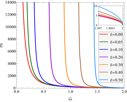
Figure 1: Dependence of the soliton energy $\tilde{E}$ on the phase frequency $\tilde{\omega}$ for several values of the gauge coupling constant $\tilde{e}$.

Figure 1 shows the dependence of the soliton energy $\tilde{E}$ on the phase frequency $\tilde{\omega}$ for several values of the gauge coupling constant $\tilde{e}$. We see that for each $\tilde{e}$, the phase frequency $\tilde{\omega}\in\left(\tilde{\omega}_{\min}(\tilde{e}),\tilde{\omega}_{\max}\right]$, where $\tilde{\omega}_{\max}=2^{-1/2}\tilde{\chi}_{1\,\text{vac}}=2$. As $\tilde{e}$ decreases, the minimum allowable frequency $\tilde{\omega}_{\min}(\tilde{e})$ falls monotonically, reaching the limiting value $\tilde{\omega}_{\min}(0)=0$. Using numerical methods, we can show that as $\tilde{\omega}\rightarrow\tilde{\omega}_{\min}(\tilde{e})$, the soliton energy

$$\tilde{E}\left(\tilde{\omega},\tilde{e}\right)\sim a(\tilde{e})(\tilde{\omega}-\tilde{\omega}_{\min}(\tilde{e}))^{-2},$$ (44)

where $a(\tilde{e})$ is a function of $\tilde{e}$. It follows that the soliton energy increases indefinitely as $\tilde{\omega}\rightarrow\tilde{\omega}_{\min}(\tilde{e})$. On the other hand, $\tilde{\omega}_{\min}(\tilde{e})$ monotonically increases with $\tilde{e}$, meaning that there is a limiting value $\tilde{e}_{\max}$ for which $\tilde{\omega}_{\min}(\tilde{e}_{\max})=\tilde{\omega}_{\max}$. It follows that the nontopological soliton can exist only when $\tilde{e}\in\left[0,\tilde{e}_{\max}\right)$.

In the subplot in Fig. 1, we can see the curves $\tilde{E}(\tilde{\omega},\tilde{e})$ in the vicinity of the maximum allowable phase frequency $\tilde{\omega}_{\max}$. All the curves $\tilde{E}(\tilde{\omega},\tilde{e})$ in the subplot tend to zero as $\tilde{\omega}\rightarrow\tilde{\omega}_{\max}$. It has been found numerically that as $\tilde{\omega}\rightarrow\tilde{\omega}_{\min}(\tilde{e})$, the soliton energy

$$\tilde{E}\left(\tilde{\omega},\tilde{e}\right)\approx b(\tilde{e})\left(\tilde{\omega}_{\max}-\tilde{\omega}\right)^{1/2},$$ (45)

where $b(\tilde{e})$ is an increasing function of $\tilde{e}$.

According to Eq. (21), the curves $\tilde{Q}_{N}(\tilde{\omega},\tilde{e})$ are related to the curves $\tilde{E}(\tilde{\omega},\tilde{e})$ by the integral relation $\tilde{Q}_{N}\left(\tilde{\omega},\tilde{e}\right)=-\int\nolimits_{\tilde{\omega}}^{\tilde{\omega}_{\max}}\tau^{-1}\partial_{\tau}\tilde{E}\left(\tau,\tilde{e}\right)d\tau$. It follows that the curves $\tilde{Q}_{N}(\tilde{\omega},\tilde{e})$ will be similar to the curves $\tilde{E}(\tilde{\omega},\tilde{e})$ shown in Fig. 1; in particular, the behavior of the curves $\tilde{Q}_{N}(\tilde{\omega},\tilde{e})$ in the neighborhoods of $\tilde{\omega}_{\min}$ and $\tilde{\omega}_{\max}$ is the same as that of the curves $\tilde{E}(\tilde{\omega},\tilde{e})$.

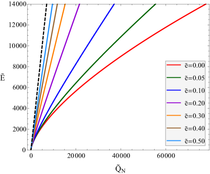
Figure 2: Dependence of the soliton energy $\tilde{E}$ on the Noether charge $\tilde{Q}_{N}$ for several values of the gauge coupling constant $\tilde{e}$.

Figure 2 shows the dependence of the soliton energy $\tilde{E}$ on the Noether charge $\tilde{Q}_{N}$ for several values of the gauge coupling constant $\tilde{e}$. In Fig. 2, the black dashed line $\tilde{E}=\tilde{\omega}_{\max}\tilde{Q}_{N}$ corresponds to the energy of a plane-wave configuration with a given Noether charge $\tilde{Q}_{N}$. We see that for all values of $\tilde{e}$ considered here, the energies of the solitons with a given $\tilde{Q}_{N}$ are lower than the energy of the corresponding plane-wave configuration. It follows that these solitons are stable against decay into massive charged $\phi$-mesons.

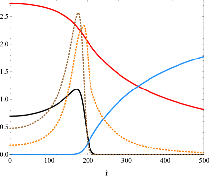
Figure 3: Scaled dimensionless functions $10\times\tilde{f}(\tilde{r})$ (solid black), $\tilde{\Phi}(\tilde{r})$ (solid red), $\tilde{\chi}_{1}(\tilde{r})$ (solid blue), $10^{4}\times\tilde{\mathcal{E}}(\tilde{r})$ (dashed orange), and $10^{3}\times\tilde{j}_{N}^{0}(\tilde{r})$ (dashed brown). The functions correspond to the parameters $\tilde{e}=0.1$ and $\tilde{\omega}=0.32214$.

We have established that the energy $\tilde{E}(\tilde{\omega},\tilde{e})$ and the Noether charge $\tilde{Q}_{N}(\tilde{\omega},\tilde{e})$ of the soliton increase indefinitely as $\tilde{\omega}\rightarrow\tilde{\omega}_{\min}(\tilde{e})$. In view of this, it would be interesting to explore the behavior of the soliton fields in this limit. To do this, we define the dimensionless profile functions $\tilde{f}(\tilde{r})=m^{-1}gf(r)$, $\tilde{\chi}_{1}(\tilde{r})=m^{-1}g\chi_{1}(r)$, and $\tilde{\Phi}(\tilde{r})=m^{-1}g\Phi(r)$, where $\tilde{r}=m^{-1}r$. We also define the dimensionless energy density $\tilde{\mathcal{E}}(\tilde{r})=m^{-4}g^{2}\mathcal{E}(r)$ and the dimensionless Noether charge density $\tilde{j}_{N}^{0}(\tilde{r})=m^{-3}g^{2}j_{N}^{0}(r)$. Figure 3 shows these dimensionless functions for parameter values $\tilde{e}=0.1$ and $\tilde{\omega}=0.32214$. Note that $\tilde{\omega}=0.32214$ is the minimum value of the phase frequency, which we were able to achieve by numerical methods for $\tilde{e}=0.1$. We see that only $\tilde{f}(\tilde{r})$ and $\tilde{j}^{0}_{N}(\tilde{r})$ are localised, whereas $\tilde{\Phi}(\tilde{r})$, $\tilde{\chi}_{1}(\tilde{r})$, and $\tilde{\mathcal{E}}(\tilde{r})$ are long-range, which is consistent with the asymptotic forms in Eqs. (24), (25), and (26). We also see that $\tilde{\chi}_{1}(\tilde{r})\approx 0$ in the interior of the soliton. The long-range character ($\propto r^{-4}$) of the energy density $\tilde{\mathcal{E}}$ arises from the gradient of the long-range electric potential $\tilde{\Phi}$ and the gradient of the long-range neutral scalar field $\tilde{\chi}_{1}$. According to Eq. (14), the local character of the charge density $\tilde{j}_{N}^{0}$ is due to the local character of the function $\tilde{f}$. Note that the electrostatic repulsion causes the electric charge density to increase near the surface of the soliton.

Eq. (25) tells us that the asymptotics of $\tilde{\chi}_{1}$ is characterised by the scalar charge $\tilde{Q}_{\text{s}}=gQ_{\text{s}}$. Using numerical methods, we find that similarly to the energy $\tilde{E}$ and the Noether charge $\tilde{Q}_{N}$, the scalar charge

$$\tilde{Q}_{\text{s}}\left(\tilde{\omega},\tilde{e}\right)\propto\left(\tilde{\omega}-\tilde{\omega}_{\min}\left(\tilde{e}\right)\right)^{-2}$$ (46)

as $\tilde{\omega}\rightarrow\tilde{\omega}_{\min}$. However, unlike the Noether (electric) charge $Q_{N}$ ($Q=eQ_{N}$), the scalar charge $Q_{\text{s}}$ is simply a definition and is not related to any symmetry of model (1).

6 Conclusion

In the present paper, we show that an electrically charged nontopological soliton exists in a version of $\mathcal{N}=1$ supersymmetric scalar electrodynamics. A characteristic feature of this soliton is the presence of two long-range fields, which slowly ($\propto r^{-1}$) tend to limiting values: these are the electrostatic Coulomb field, and the electrically neutral massless scalar field. The presence of these two long-range fields leads to a modification of the intersoliton interaction in comparison with the purely Coulomb case. Another feature of the soliton is that its energy and electric charge take arbitrarily large values when the modulus of the phase frequency tends to the minimum possible value. In contrast, the energy and electric charge of the soliton vanish when the modulus of the phase frequency tends to the maximum possible value.

We note that in the general case, the energy and electric charge of a nontopological soliton cannot be arbitrarily large due to Coulomb repulsion [10, 20]. We avoid this restriction because the attraction due to the massless scalar field compensates for the Coulomb repulsion. A similar situation also arises in the massless limit of the gauged Fridberg-Lee-Sirlin model [21, 23]. It is also worth noting that the electric charge and energy of the dyon (electrically charged magnetic monopole) also cannot be arbitrarily large in the general non-BPS case [35]. Only in the BPS limit, when the scalar field of the dyon becomes massless, can the energy and electric charge take arbitrarily large values.

The $\mathcal{N}=1$ supersymmetry of the model makes it possible to obtain expressions for the fermionic zero modes in terms of bosonic fields of the soliton. The fermionic zero modes are bound states of the fermion-soliton system, and their components that correspond to the long-range bosonic fields are also long-range. In accordance with the number of $\mathcal{N}=1$ supersymmetry generators, the number of independent fermionic zero modes of the soliton is four. The fermionic zero modes of two solitons with opposite electric charges are related by the $CP$ transformation.

In this work, we have investigated a nontopological soliton of an $\mathcal{N}=1$ supersymmetric Abelian gauge model. It is known [36, 37], however, that nontopological solitons can also exist in non-Abelian gauge models. In particular, it was shown in Ref. [38] that an electrically charged nontopological soliton exists in the Weinberg-Salam model of electroweak interactions. This model allows for $\mathcal{N}=1$ supersymmetric extension, and its fermionic sector contains both massive ($e$, $\mu$, $\tau$) and massless ($\nu_{e}$, $\nu_{\mu}$, $\nu_{\tau}$) fermions. The bosonic superpartners of the neutrinos (sneutrinos) also have zero masses. We can assume that, similarly to the nonsupersymmetric case [38], an electrically charged nontopological soliton also exists in this model, meaning that some properties of this soliton will be similar to those studied in this work. In particular, in addition to the long-range Coulomb field, this soliton will have long-range fields of massless sneutrinos. Furthermore, it will be possible to express the fermionic zero modes of this soliton in terms of its bosonic fields.

Figure captions

Fig. 1. Dependence of the soliton energy $\tilde{E}$ on the phase frequency $\tilde{\omega}$ for several values of the gauge coupling constant $\tilde{e}$.

Fig. 2. Dependence of the soliton energy $\tilde{E}$ on the Noether charge $\tilde{Q}_{N}$ for several values of the gauge coupling constant $\tilde{e}$.

Fig. 3. Scaled dimensionless functions $10\times\tilde{f}(\tilde{r})$ (solid black), $\tilde{\Phi}(\tilde{r})$ (solid red), $\tilde{\chi}_{1}(\tilde{r})$ (solid blue), $10^{4}\times\tilde{\mathcal{E}}(\tilde{r})$ (dashed orange), and $10^{3}\times\tilde{j}_{N}^{0}(\tilde{r})$ (dashed brown). The functions correspond to the parameters $\tilde{e}=0.1$ and $\tilde{\omega}=0.32214$.

References

- [1] N. Manton, P. Sutclffe, Topological Solitons, Cambridge University Press, Cambridge, 2004.
- [2] V. Rubakov, Classical Theory of Gauge Fields, Princeton University Press, Princeton, 2002.
- [3] T. D. Lee, Y. Pang, Phys. Rep. 221 (1992) 251. doi:10.1016/0370-1573(92)90064-7.
- [4] S. Coleman, Nucl. Phys. B 262 (1985) 263. doi:/10.1016/0550-3213(85)90286-X.
- [5] F. P. Correia, M. Schmidt, Eur. Phys. J. C 21 (2001) 181. doi:10.1007/s100520100710.
- [6] A. Kusenko, Phys. Lett. B 406 (1997) 26. doi:10.1016/S0370-2693(97)00700-4.
- [7] I. Affleck, M. Dine, Nucl. Phys. B 249 (1985) 361. doi:10.1016/0550-3213(85)90021-5.
- [8] A. Kusenko, M. Shaposhnikov, Phys. Lett. B 418 (1998) 46. doi:10.1016/S0370-2693(97)01375-0.
- [9] G. Rosen, J. Math. Phys. (N.Y.) 9 (1968) 999. doi:/10.1063/1.1664694.
- [10] K. Lee, J. A. Stein-Schabes, R. Watkins, L. M. Widrow, Phys. Rev. D 39 (1989) 1665. doi:10.1103/PhysRevD.39.1665.
- [11] C. H. Lee, S. U.Yoon, Mod. Phys. Lett. A 6 (1991) 1479. doi:10.1142/S0217732391001597.
- [12] K. N. Anagnostopoulos, M. Axenides, E. G. Floratos, N. Tetradis, Phys. Rev. D 64 (2001) 125006. doi:10.1103/PhysRevD.64.125006.
- [13] T. S. Levi, M. Gleiser, Phys. Rev. D 66 (2002) 087701. doi:10.1103/PhysRevD.66.087701.
- [14] E. Radu, M. Volkov, Phys. Rep. 468 (2008) 101. doi:10.1016/j.physrep.2008.07.002.
- [15] H. Arodz, J. Lis, Phys. Rev. D 79 (2009) 045002. doi:10.1103/PhysRevD.79.045002.
- [16] T. Tamaki, N. Sakai, Phys. Rev. D 90 (2014) 085022. doi:10.1103/PhysRevD.90.085022.
- [17] I. E. Gulamov, E. Y. Nugaev, M. N. Smolyakov, Phys. Rev. D 89 (2014) 085006. doi:10.1103/PhysRevD.89.085006.
- [18] Y. Brihaye, V. Diemer, B. Hartmann, Phys. Rev. D 89 (2014) 084048. doi:10.1103/PhysRevD.89.084048.
- [19] J.-P. Hong, M. Kawasaki, M. Yamada, Phys. Rev. D 92 (2015) 063521. doi:10.1103/PhysRevD.92.063521.
- [20] I. E. Gulamov, E. Y. Nugaev, A. G. Panin, M. N. Smolyakov, Phys. Rev. D 92 (2015) 045011. doi:10.1103/PhysRevD.92.045011.
- [21] V. Loiko, Ya. Shnir, Phys. Lett. B 797 (2019) 134810. doi:10.1016/j.physletb.2019.134810.
- [22] A. Yu. Loginov, V. V. Gauzshtein, Phys. Rev. D 102 (2020) 025010. doi:10.1103/PhysRevD.102.025010.
- [23] V. Loiko, Ya. Shnir, Phys. Rev. D 106 (2022) 045021. doi:10.1103/PhysRevD.106.045021.
- [24] S. Weinberg, The Quantum Theory of Fields, Vol.3: Supersymmetry, Cambridge University Press, Cambridge, 2000.
- [25] J. Wess, B. Zumino, Nucl. Phys. B 70 (1974) 39. doi:10.1016/0550-3213(74)90355-1.
- [26] A. Yu. Loginov, Phys. At. Nucl. 73 (2010) 448. doi:10.1134/S1063778810030075.
- [27] M. T. Grisaru, W. Siegel, M. Rǒcek, Nucl. Phys. B 159 (1979) 429. doi:10.1016/0550-3213(79)90344-4.
- [28] N. Seiberg, Phys. Lett. B 318 (1993) 469. doi:10.1016/0370-2693(93)91541-T.
- [29] A. Yu. Loginov, Phys. Lett. B 822 (2021) 136662. doi:10.1016/j.physletb.2021.136662.
- [30] A. Levin, V. Rubakov, Mod. Phys. Lett. A 26 (2011) 409. doi:10.1142/S0217732311034992.
- [31] V. Loiko, I. Perapechka, Ya. Shnir, Phys. Rev. D 98 (2018) 045018. doi:10.1103/PhysRevD.98.045018.
- [32] J. Kunz, V. Loiko, Ya. Shnir, Phys. Rev. D 105 (2022) 085013. doi:10.1103/PhysRevD.105.085013.
- [33] B. de Wit, D. Z. Freedman, Phys. Rev. D 12 (1975) 2286. doi:10.1103/PhysRevD.12.2286.
- [34] Maple User Manual, (Maplesoft, Waterloo, Canada, 2019).
- [35] Y. Brihaye, B. Kleihaus, D. H. Tchrakian, J. Math. Phys. 40 (1999) 1136. doi:10.1063/1.532793.
- [36] R. Friedberg, T. D. Lee, A. Sirlin, Nucl. Phys. B 115 (1976) 1. doi:10.1016/0550-3213(76)90274-1.
- [37] R. Friedberg, T. D. Lee, A. Sirlin, Nucl. Phys. B 115 (1976) 32. doi:10.1016/0550-3213(76)90275-3.
- [38] A. Yu. Loginov, JETP 114 (2012) 48. doi:10.1134/S1063776111150076.