A space-time finite element method for the eddy current approximation of rotating electric machines

Abstract

In this paper we formulate and analyze a space-time finite element method for the numerical simulation of rotating electric machines where the finite element mesh is fixed in space-time domain. Based on the Babuška–Nečas theory we prove unique solvability both for the continuous variational formulation and for a standard Galerkin finite element discretization in the space-time domain. This approach allows for an adaptive resolution of the solution both in space and time, but it requires the solution of the overall system of algebraic equations. While the use of parallel solution algorithms seems to be mandatory, this also allows for a parallelization simultaneously in space and time. This approach is used for the eddy current approximation of the Maxwell equations which results in an elliptic-parabolic interface problem. Numerical results for linear and nonlinear constitutive material relations confirm the applicability, efficiency and accuracy of the proposed approach.

1 Introduction

Electric machines have become an integral part of everyday life with a large share of global electric energy being converted into mechanical energy by electric machines. The efficient and accurate numerical simulation of electric machines is thus an important topic in particular in order to design new machines with high performance indicators. Mathematical models for computing the magnetic flux density and the magnetic field inside an electric machine are based on low-frequency approximations to Maxwell’s equations such as the magneto-quasi-static or the magneto-static approximations. While the former accounts for eddy currents in conducting regions and is also refered to as the eddy current approximation of Maxwell’s equations [26], the more widely used magneto-static approximation ignores these effects. Eddy currents yield thermal losses [14] and thus are typically an unwanted effect in electric machines and therefore often counteracted, e.g., by assembling the machine from thin laminated steel sheets. Nevertheless, these effects are still present, e.g., in permanent magnets or when non-laminated designs are chosen [20], and their accurate computation is of high relevance. While the magneto-static approximation to Maxwell’s equations for rotating electric machines results in a sequence of independent static problems, the eddy current approximation yields a time-dependent problem of mixed parabolic-elliptic type [3]. This type of problems is typically solved by frequency domain methods such as the multi-harmonic finite element method [38] or the harmonic balance method [13, 25], or by classical time-stepping methods in time domain [36]. Since classical time-stepping methods suffer from the curse of sequentiality, different ways to employ parallelization also in time direction have been investigated over the past decades [9] including shooting methods, domain decomposition or multigrid methods [11] in time. We mention the application of parareal [10, 15] and multigrid reduction in time [4, 8] algorithms to the time-parallel simulation of eddy current problems for electric machines.

On the other hand, space-time finite element methods [33] for the numerical solution of time-dependent partial differential equations have gained increasing attention over the past decade due to increasing computing capabilities. Here, the idea is to treat the time variable like an additional space variable and to construct a $(d+1)$-dimensional space-time mesh when the spatial domain is in $\mathbb{R}^{d}$. In this setting, a moving domain can conveniently be captured by the space-time mesh. While, at the first glance, the method comes with the challenge of higher-dimensional linear systems to be solved, it allows for both parallelization [11] and adaptivity [18, 32] not only in space or time, but also in space-time. Moreover, in the context of optimization problems with partial differential equations as constraint, and involving an adjoint state which is directed backward in time, space-time methods allow for an additional level of parallelism by solving the coupled system for the state and the adjoint in parallel [19]. Finally, we will see that for space-time finite element methods temporal periodicity conditions as they appear for rotating electric machines at a fixed operating point can be incorporated in a straightforward manner.

The numerical analysis of space-time variational formulations for parabolic evolution equations in Bochner spaces is based on the Babuška–Nečas theory [2, 22] which requires the proof of an inf-sup stability condition to ensure uniqueness, and of a surjectivity condition to ensure existence of a solution. In the context of space-time finite element methods this was done in [28], see also [1, 30, 37]. Alternatively, one may use isogeometric space-time finite element methods [16], least squares formulations [35], or a Galerkin space-time finite element method in anisotropic Sobolev spaces [34].

In this paper, we extend the analysis of [30], which is based on the Babuška–Nečas theorem, to the case of a coupled elliptic-parabolic partial differential equation which is formulated in a spatial domain which is changing in time. In particular we will restrict ourselves to the case of a rotating subdomain as it is the case for rotating electric machines. While we exploit this property in our proof of surjectivity of the bilinear form (Lemma 3.1), we claim that the presented approach can also be applied in more general settings, also including compressible deformations of the computational domain.

The rest of this paper is organized as follows: In Section 2, starting out from Maxwell’s equations, we derive the mathematical model of two-dimensional magneto-quasi-statics which we consider in the sequel. The main part of this paper is Section 3 where we verify the conditions of the Babuška–Nečas theorem and conclude existence of a unique solution. In Section 4 we introduce a space-time finite element discretization and give the corresponding stability and error estimates before resorting to numerical experiments in Section 5, where we also discuss the parallel solution of the algebraic equations. In addition to the linear model problem we also include a nonlinear model to describe the reluctivity in iron. Finally, we summarize and comment on ongoing and future work.

2 Model description

To model the electromagnetic fields in a rotating electric machine, e.g., an electric motor, we consider the eddy current approximation of the Maxwell equations, see, e.g., [17],

$$\text{curl}_{y}H(y,t)=J(y,t),\quad\text{curl}_{y}E(y,t)=-\partial_{t}B(y,t),\quad\text{div}_{y}B(y,t)=0,$$ (2.1)

subject to the constitutive equations

$$B(y,t)=\mu(y)H(y,t)+M(y,t),\quad J(y,t)=J_{i}(y,t)+\sigma(y)\Big{[}E(y,t)+v(y,t)\times B(y,t)\Big{]},$$ (2.2)

where $\mu$ is the material dependent magnetic permeability, $\sigma$ is the electric conductivity, $J_{i}$ is an impressed electric current, $M$ is the magnetization which vanishes outside permanent magnets, and $v=\frac{d}{dt}y(t)$ is the velocity along the trajectory $y(t)=\varphi(t,x)\in{\mathbb{R}}^{3}$ for a reference point $x\in{\mathbb{R}}^{3}$. We assume that the deformation $\varphi$ is bijective and sufficiently regular for all $t\in(0,T)$, satisfying $\varphi(0,x)=x$. Here, $T>0$ is a given time horizon, and we assume that $\text{div}_{y}v(y,t)=0$.

When using the vector potential ansatz $B=\text{curl}_{y}A$ satisfying $\text{div}_{y}B=\text{div}_{y}\text{curl}_{y}A=0$, we can rewrite the second equation in (2.1) as $0=\text{curl}_{y}E+\partial_{t}B=\text{curl}_{y}[E+\partial_{t}A]$, which implies, recall that the vector potential $A$ is unique up to a gradient field only, $E=-\partial_{t}A$. When using the reluctivity $\nu=1/\mu$ we then have $H=\nu(B-M)=\nu(\text{curl}_{y}A-M)$ in order to rewrite the first equation in (2.1) as

$$\text{curl}_{y}\Big{[}\nu(y)\Big{(}\text{curl}_{y}A(y,t)-M(y,t)\Big{)}\Big{]}=J_{i}(y,t)-\sigma(y)\Big{[}\partial_{t}A(y,t)+\text{curl}_{y}A(y,t)\times v(y,t)\Big{]}.$$ (2.3)

Assuming that

$$H(y,t)=(H_{1}(y_{1},y_{2},t),H_{2}(y_{1},y_{2},t),0)^{\top},\quad M(y,t)=(M_{1}(y_{1},y_{2},t),M_{2}(y_{1},y_{2},t),0)^{\top},$$

and

$$v(y,t)=(v_{1}(y_{1},y_{2},t),v_{2}(y_{1},y_{2},t),0)^{\top},\quad J_{i}(y,t)=(0,0,j_{i}(y_{1},y_{2},t))^{\top},$$

which is often (approximately) the case for electric machines, it follows that $A=(0,0,u(y_{1},y_{2},t))^{\top}$, and we can consider a spatially two-dimensional reference domain $\Omega\subset{\mathbb{R}}^{2}$ describing the cross-section of the electric motor. Using $x=(x_{1},x_{2},0)^{\top}$ for $(x_{1},x_{2})\in\Omega$, we can rewrite (2.3) as

$$\sigma(y_{1},y_{2})\frac{d}{dt}u(y_{1},y_{2},t)-\text{div}_{(y_{1},y_{2})}[\nu(y_{1},y_{2})\nabla_{(y_{1},y_{2})}u(y_{1},y_{2},t)]$$ (2.4)

$$\hskip 113.81102pt=j_{i}(y_{1},y_{2},t)-\text{div}_{(y_{1},y_{2})}[\nu(y_{1},y_{2})M^{\perp}(y_{1},y_{2},t)],$$

where

$$\frac{d}{dt}u(y_{1},y_{2},t):=\partial_{t}u(y_{1},y_{2},t)+v(y_{1},y_{2},t)\cdot\nabla_{(y_{1},y_{2})}u(y_{1},y_{2},t)$$

is the total time derivative, and $M^{\perp}=(-M_{2}(y_{1},y_{2},t),M_{1}(y_{1},y_{2},t))^{\top}$ is the perpendicular of the first two components of the magnetization $M$. In addition to the partial differential equation (2.4) we consider homogeneous Dirichlet boundary conditions $u=0$ on $\partial\Omega\times(0,T)$ which implies that $B\cdot n=0$ on $\partial\Omega\times(0,T)$, i.e., no magnetic flux leaves the computational domain, and either the initial condition $u(x_{1},x_{2},0)=0$ or the periodicity condition $u(x_{1},x_{2},T)=u(x_{1},x_{2},0)$, both for $(x_{1},x_{2})\in\Omega$ when $\sigma(x_{1},x_{2})>0$. Note that, in the case of periodicity conditions, we assume that also the geometry and the sources are periodic with respect to the period $T$.

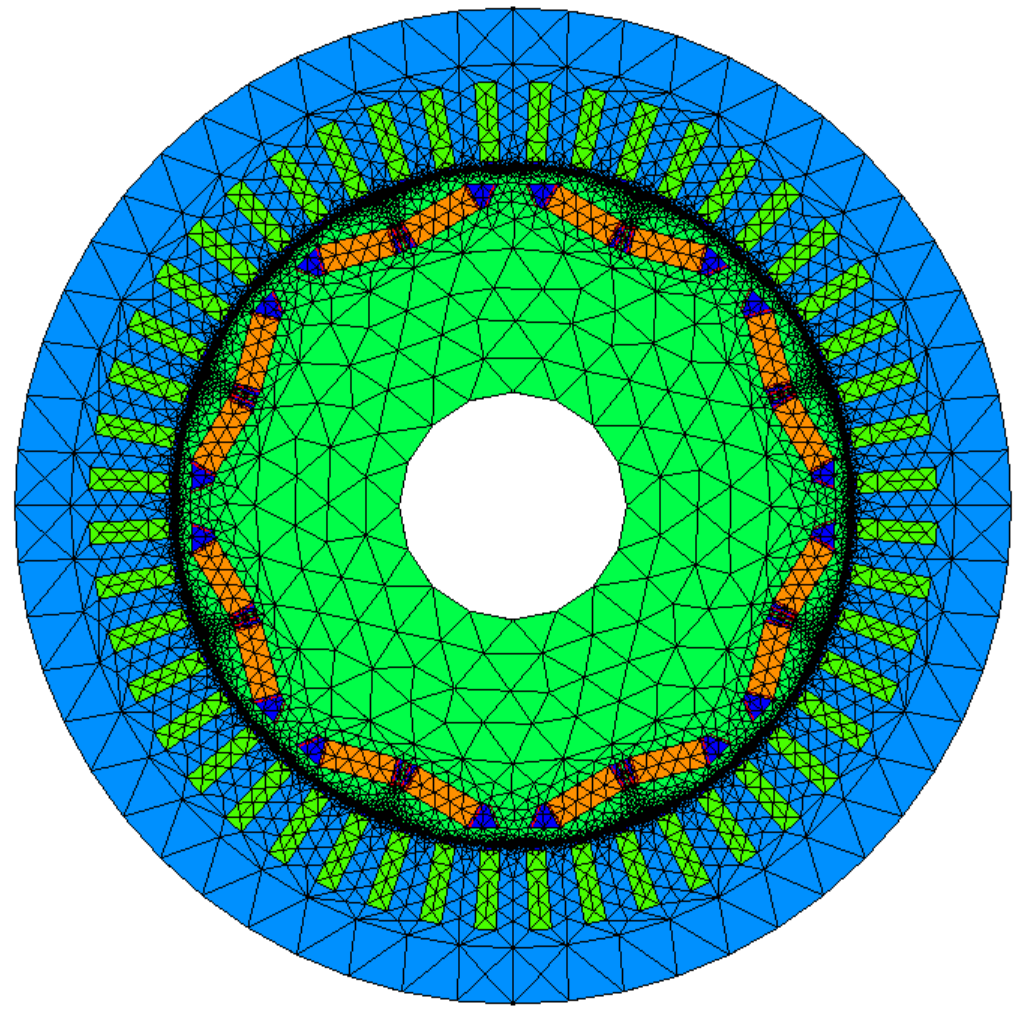
Figure 1: Finite element mesh of the reference domain $\Omega$ describing an electric motor with the stator $\Omega_{s}$ including the coils, the rotor domain $\Omega_{r}=\Omega_{r}(t)$ including the magnets and surrounding air pockets, and the thin air gap $\Omega_{air}$ separating $\Omega_{r}$ from $\Omega_{s}$.

We consider an electric motor as shown in Fig. 1 which consists of a rotor in $\Omega_{r}(t)$, the stator in $\Omega_{s}$, and the air domain $\Omega_{air}$ which is non-conducting, i.e., $\sigma=0$ in $\Omega_{air}$. In this case, the evolution equation (2.4) degenerates to a coupled parabolic-elliptic interface problem. Within the stator there are $48$ coils excited with a current and which are considered to be non-conducting, since certain materials are used to ensure this property. We furthermore denote the union of all non-conducting regions ($\sigma=0$) by $\Omega_{non}$, and the regions with conducting material ($\sigma>0$) by $\Omega_{con}$. The stator in $\Omega_{s}$ is fixed, i.e., $y=\varphi(t,x)=x$ for all $t\in(0,T)$ implying $v\equiv 0$, but the rotor and the magnets within the rotor are rotating.

To cover all different regions, i.e., rotor, stator, and air, in a unified framework, we use polar coordinates to write $(x_{1},x_{2})^{\top}=r(\cos\phi,\sin\phi)^{\top}\in\Omega$ for $\phi\in[0,2\pi)$ and $r\in(r_{0},R)$, where $r_{0}$ and $R$ are the interior and exterior radii of the motor, respectively. In addition, for $r\in(r_{0},r_{1})$ we describe the rotor in the domain $\Omega_{r}(t)$ which is rotating with a velocity $\alpha$, and which may contain non-conducting areas such as air as well, while for $r\in(r_{1},r_{2})$ we have the stator domain $\Omega_{s}$ which is fixed in time. In the remaining ring domain $r\in(r_{1},r_{2})$ we model non-conducting air in $\Omega_{air}$. When using

$$\psi(r)=\left\{\begin{array}[]{cl}1&\mbox{for}\;r\in(r_{0},r_{1}),\\[5.69054pt] \displaystyle\frac{r_{2}-r}{r_{2}-r_{1}}&\mbox{for}\;r\in(r_{1},r_{2}),\\[8.53581pt] 0&\mbox{for}\;r\in(r_{2},R),\end{array}\right.$$

we can introduce the deformation

$$y(t)=\varphi(t,x)=\begin{pmatrix}y_{1}(t)\\[5.69054pt] y_{2}(t)\end{pmatrix}=\,r\,\begin{pmatrix}\cos\Big{(}\phi+\alpha\,\psi(r)t\Big{)}\\[2.84526pt] \sin\Big{(}\phi+\alpha\psi(r)t\Big{)}\end{pmatrix}\in\Omega(t)\;\mbox{for}\;t\in(0,T)$$ (2.5)

which is a rotation of velocity $\alpha$ in the rotor, and which is fixed in the stator. Here, $\Omega(t):=\varphi(t,\Omega)$ represents the moving domain at time $t\in[0,T]$, and likewise we will use $\Omega_{r}(t)$, $\Omega_{non}(t)$ and $\Omega_{con}(t)$. In general, the velocity is given as

$$v(y,t)=\frac{d}{dt}y(t)\,=\,\alpha\,\psi(r)\,r\,\begin{pmatrix}-\sin\left(\phi+\alpha\,\psi(r)\,t\right)\\[2.84526pt] \cos\left(\phi+\alpha\,\psi(r)\,r\right)\end{pmatrix}=\,\alpha\,\psi(r)\,\begin{pmatrix}-y_{2}(t)\\[5.69054pt] y_{1}(t)\end{pmatrix}.$$

A simple calculation shows, recall $r=\sqrt{y_{1}^{2}+y_{2}^{2}}$, that

$$\frac{\partial}{\partial y_{1}}v_{1}(y,t)=-\alpha\,y_{2}\,\psi^{\prime}(r)\,\frac{y_{1}}{\sqrt{y_{1}^{2}+y_{2}^{2}}},\quad\frac{\partial}{\partial y_{2}}v_{2}(y,t)=\alpha\,y_{1}\,\psi^{\prime}(r)\,\frac{y_{2}}{\sqrt{y_{1}^{2}+y_{2}^{2}}},$$

and hence, $\text{div}_{(y_{1},y_{2})}v(y_{1},y_{2},t)=0$ follows. With this we can write Reynold’s transport theorem as

$$\frac{d}{dt}\int_{\Omega(t)}u(y_{1},y_{2},t)\,dy_{1}dy_{2}=\int_{\Omega(t)}\Big{(}\partial_{t}u(y_{1},y_{2},t)+\text{div}_{(y_{1},y_{2})}[u(y_{1},y_{2},t)\,v(y_{1},y_{2},t)]\Big{)}\,dy_{1}dy_{2}$$

$$=\int_{\Omega(t)}\Big{(}\partial_{t}u(y_{1},y_{2},t)+u(y_{1},y_{2},t)\,\text{div}_{(y_{1},y_{2})}v(y_{1},y_{2},t)+v(y_{1},y_{2},t)\cdot\nabla_{(y_{1},y_{2})}u(y_{1},y_{2},t)\Big{)}\,dy_{1}dy_{2}$$

$$=\int_{\Omega(t)}\Big{(}\partial_{t}u(y_{1},y_{2},t)+v(y_{1},y_{2},t)\cdot\nabla_{(y_{1},y_{2})}u(y_{1},y_{2},t)\Big{)}\,dy_{1}dy_{2}$$

$$=\int_{\Omega(t)}\frac{d}{dt}u(y_{1},y_{2},t)\,dy_{1}dy_{2}\,.$$ (2.6)

3 Space-time variational formulation

We consider the evolution equation

$$\sigma(y)\frac{d}{dt}u(y,t)-\mbox{div}_{y}[\nu(y)\nabla_{y}u(y,t)]=j_{i}(y,t)-\mbox{div}_{y}[\nu(y)M^{\bot}(y,t)]\quad\mbox{for}\;(y,t)\in Q,$$ (3.1)

where the space-time domain $Q$ is given by the deformation (2.5) as

$$Q:=\Big{\{}(y,t)\in{\mathbb{R}}^{3}:y=\varphi(t,x)\in\Omega(t),\,x\in\Omega\subset{\mathbb{R}}^{2},\,t\in(0,T)\Big{\}},$$

with homogeneous Dirichlet boundary conditions $u(x,t)=0$ for $(y,t)\in\partial\Omega(t)\times(0,T)$, and with either the initial condition $u(x,0)=0$ or the periodicity condition $u(x,T)=u(x,0)$ for $x\in\Omega\backslash\Omega_{non}$. Note that the partial differential equation (3.1) covers both conducting ($\sigma>0$) and non-conducting materials ($\sigma=0$), and the case of a fixed domain $(v=0)$ as well as the rotating regions.

In order to introduce a variational formulation of (3.1) in the space-domain $Q$ we first define the Bochner space $Y:=L^{2}(0,T;H^{1}_{0}(\Omega(t))$ covering the homogeneous Dirichlet boundary conditions, equipped with the norm

$$\|z\|_{Y}^{2}:=\int_{0}^{T}\int_{\Omega(t)}\nu(y)\,|\nabla_{y}z(y,t)|^{2}\,dy\,dt\,,$$

and the ansatz space

$$X:=\left\{u\in Y:\sigma\frac{d}{dt}u\in Y^{*},\;u(x,0)=0\text{ for }x\in\Omega_{con}\right\}\subset Y,$$

in the case of homogeneous initial conditions, or

$$X:=\left\{u\in Y:\sigma\frac{d}{dt}u\in Y^{*},\;u(x,T)=u(x,0)\text{ for }x\in\Omega_{con}\right\}\subset Y$$

in the case of a periodic behavior. The graph norm in $X$ is given in both cases as

$$\|u\|_{X}^{2}:=\|u\|_{Y}^{2}+\|\sigma\frac{d}{dt}u\|_{Y^{*}}^{2}=\|u\|^{2}_{Y}+\|w_{u}\|^{2}_{Y},$$

where $w_{u}\in Y$ is the unique solution of the variational formulation

$$\int_{0}^{T}\int_{\Omega(t)}\nu\,\nabla_{y}w_{u}\cdot\nabla_{y}z\,dy\,dt=\int_{0}^{T}\int_{\Omega(t)}\sigma\,\frac{d}{dt}u\,z\,dy\ dt\quad\mbox{for all}\;z\in Y.$$ (3.2)

Now, the space-time variational formulation of the evolution equation (3.1) is to find $u\in X$ such that

$$b(u,z):=\int_{0}^{T}\int_{\Omega(t)}\left[\sigma\,\frac{d}{dt}u\,z+\nu\,\nabla_{y}u\cdot\nabla_{y}z\right]\,dy\,dt=\int_{0}^{T}\int_{\Omega(t)}\left[j_{i}\,z+M^{\perp}\cdot\nabla_{y}z\right]\,dy\,dt$$ (3.3)

is satisfied for all $z\in Y$. As in the case of a fixed domain $\Omega$, see [30], we conclude that the bilinear form $b(\cdot,\cdot)$ is bounded, satisfying

$$|b(u,z)|\,\leq\,\sqrt{2}\,\|u\|_{X}\,\|z\|_{Y}\quad\mbox{for all}\;u\in X,z\in Y.$$

Moreover, similar as in [30] and due to (2.6) we can prove that the bilinear form $b(\cdot,\cdot)$ satisfies the inf-sup stability condition

$$\frac{1}{\sqrt{2}}\,\|u\|_{X}\leq\sup\limits_{0\neq z\in Y}\frac{b(u,z)}{\|z\|_{Y}}\quad\mbox{for all}\;u\in X\,.$$ (3.4)

Indeed, for any given $u\in X$ let $w_{u}\in Y$ be the unique solution of the variational formulation (3.2). Due to $X\subset Y$ we can consider $z_{u}:=u+w_{u}\in Y$ to obtain, when using (3.2) twice,

$$b(u,z_{u}) = b(u,u+w_{u})\,=\,\int_{0}^{T}\int_{\Omega(t)}\sigma\frac{d}{dt}u\,u\,dy\,dt+\int_{0}^{T}\int_{\Omega(t)}\nu\,\nabla_{y}u\cdot\nabla_{y}u\,dy\,dt$$

$$\hskip 71.13188pt+\int_{0}^{T}\int_{\Omega(t)}\sigma\frac{d}{dt}u\,w_{u}\,dy\,dt+\int_{0}^{T}\int_{\Omega(t)}\nu\,\nabla_{y}u\cdot\nabla_{y}w_{u}\,dy\,dt$$

$$=\,2\int_{0}^{T}\int_{\Omega(t)}\sigma\frac{d}{dt}u\,u\,dy\,dt+\int_{0}^{T}\int_{\Omega(t)}\nu\,\nabla_{y}u\cdot\nabla_{y}u\,dy\,dt+\int_{0}^{T}\int_{\Omega(t)}\nu\,\nabla_{y}w_{u}\cdot\nabla_{y}w_{u}\,dy\,dt$$

$$=\int_{0}^{T}\int_{\Omega(t)}\sigma\,\frac{d}{dt}[u]^{2}\,dy\,dt+\|u\|_{Y}^{2}+\|w_{u}\|^{2}_{Y}\,\geq\,\|u\|_{X}^{2}\,.$$

Note that, since $\sigma$ is constant in time, we can use (2.6) to conclude

$$\int_{0}^{T}\int_{\Omega(t)}\sigma\,\frac{d}{dt}[u]^{2}\,dy\,dt = \int_{0}^{T}\frac{d}{dt}\int_{\Omega(t)}\sigma\,[u]^{2}\,dy\,dt\,=\,\left.\int_{\Omega(t)}\sigma(y)\,[u(y,t)]^{2}\,dy\right|_{0}^{T}$$

$$= \int_{\Omega_{con}(T)}\sigma(y)\,[u(y,T)]^{2}\,dy\,>\,0$$

in the case of initial conditions $u(x,0)=0$ for $x\in\Omega_{con}(0)$, or

$$\int_{0}^{T}\int_{\Omega(t)}\sigma\,\frac{d}{dt}[u]^{2}\,dy\,dt\,=\,\int_{\Omega_{con}(T)}\sigma(y)\,[u(y,T)]^{2}\,dy-\int_{\Omega_{con}(0)}\sigma(y)\,[u(y,0)]^{2}\,dy\,=\,0$$

in the case of periodicity $u(x,T)=u(x,0)$.

On the other hand, by the triangle and Hölder inequality we have

$$\|z_{u}\|_{Y}=\|u+w_{u}\|_{Y}\leq\|u\|_{Y}+\|w_{u}\|_{Y}\leq\sqrt{2}\,\sqrt{\|u\|_{Y}^{2}+\|w_{u}\|_{Y}^{2}}=\sqrt{2}\,\|u\|_{X},$$

i.e.,

$$b(u,z_{u})\,\geq\,\|u\|_{X}^{2}\,\geq\,\frac{1}{\sqrt{2}}\,\|u\|_{X}\|z_{u}\|_{Y}$$

implies the inf-sup stability condition (3.4).

More involved, and not as simple as in the static case, is to prove that the bilinear form $b(\cdot,\cdot)$ is also surjective.

Lemma 3.1

For all $z\in Y\backslash\{0\}$ there exists a $\widetilde{u}\in X$ such that

$$b(\widetilde{u},z)\neq 0\,.$$

Proof. We first consider the case of initial conditions $u(x,0)=0$ for $x\in\Omega_{con}$. Using the representation (2.5) and for given $z\in Y\backslash\{0\}$ we first define

$$\widetilde{u}(y,t)=\widetilde{u}(\varphi(t,x),t):=\int_{0}^{t}z(\varphi(s,x),s)\,ds,\quad\frac{d}{dt}\widetilde{u}(y,t)=z(y,t)\quad\mbox{for}\;y\in\Omega_{con}(t),t\in(0,T).$$

By definition we have $\widetilde{u}\in X$ satisfying the initial condition $\widetilde{u}(x,0)=0$ for $x\in\Omega_{con}$ and

$$b(\widetilde{u},z) = \int_{0}^{T}\int_{\Omega(t)}\sigma(y)\frac{d}{dt}\widetilde{u}(y,t)\,z(y,t)\,dy\,dt+\int_{0}^{T}\int_{\Omega(t)}\nu(y)\,\nabla_{y}\widetilde{u}(y,t)\cdot\nabla_{y}z(y,t)\,dy\,dt$$

$$= \int_{0}^{T}\int_{\Omega_{con}(t)}\sigma(y)\,[z(y,t)]^{2}\,dy\,dt+\int_{0}^{T}\int_{\Omega(t)}\nu(y)\,\nabla_{y}\widetilde{u}(y,t)\cdot\nabla_{y}\frac{d}{dt}\widetilde{u}(y,t)\,dy\,dt\,.$$

Since the first term is obviously positive, it remains to treat the second term which involves an integral over $\Omega(t)=(\Omega_{s}\cap\Omega_{con})\cup(\Omega_{r}(t)\cap\Omega_{con}(t))\cup\Omega_{non}(t)$. In the stator domain $\Omega_{s}$, i.e., for $r\in(r_{2},R)$, we have $y(t)=x$ for all $t\in(0,T)$ and $v(y,t)=0$, and hence

$$\int_{0}^{T}\int_{\Omega_{s}\cap\Omega_{con}}\nu(x)\,\nabla_{x}\widetilde{u}_{s}(x,t)\cdot\nabla_{x}\partial_{t}\widetilde{u}_{s}(x,t)\,dx\,dt = \frac{1}{2}\int_{0}^{T}\frac{d}{dt}\int_{\Omega_{s}\cap\Omega_{con}}\nu(x)\,|\nabla_{x}\widetilde{u}_{s}(x,t)|^{2}dx\,dt$$

$$= \frac{1}{2}\int_{\Omega_{s}\cap\Omega_{con}}\nu(x)\,|\nabla_{x}\widetilde{u}_{s}(x,T)|^{2}dx\geq 0\,.$$

Next we consider the rotor domain $\Omega_{r}(t)$, i.e., $r\in(r_{0},r_{1})$. For the total time derivative we then obtain

$$\frac{d}{dt}\widetilde{u}(y,t) = \frac{\partial}{\partial t}\widetilde{u}(y,t)+v(y,t)\cdot\nabla_{y}\widetilde{u}(y,t)$$

$$= \frac{\partial}{\partial t}\widetilde{u}(y,t)-\alpha\,y_{2}\frac{\partial}{\partial y_{1}}\widetilde{u}(y,t)+\alpha\,y_{1}\frac{\partial}{\partial y_{2}}\widetilde{u}(y,t).$$

To compute the spatial gradient, we now consider

$$\frac{\partial}{\partial y_{1}}\frac{d}{dt}\widetilde{u}(y,t) = \frac{\partial}{\partial y_{1}}\left[\frac{\partial}{\partial t}\widetilde{u}(y,t)-\alpha\,y_{2}\frac{\partial}{\partial y_{1}}\widetilde{u}(y,t)+\alpha\,y_{1}\frac{\partial}{\partial y_{2}}\widetilde{u}(y,t)\right]$$

$$= \frac{\partial}{\partial y_{1}}\frac{\partial}{\partial t}\widetilde{u}(y,t)-\alpha\,y_{2}\frac{\partial^{2}}{\partial y_{1}^{2}}\widetilde{u}(y,t)+\alpha\,y_{1}\frac{\partial}{\partial y_{1}}\frac{\partial}{\partial y_{2}}\widetilde{u}(y,t)+\alpha\,\frac{\partial}{\partial y_{2}}\widetilde{u}(y,t)$$

$$= \frac{\partial}{\partial t}\frac{\partial}{\partial y_{1}}\widetilde{u}(y,t)-\alpha\,y_{2}\frac{\partial^{2}}{\partial y_{1}^{2}}\widetilde{u}(y,t)+\alpha\,y_{1}\frac{\partial}{\partial y_{2}}\frac{\partial}{\partial y_{1}}\widetilde{u}(y,t)+\alpha\,\frac{\partial}{\partial y_{2}}\widetilde{u}(y,t)$$

$$= \frac{d}{dt}\frac{\partial}{\partial y_{1}}\widetilde{u}(y,t)+\alpha\,\frac{\partial}{\partial y_{2}}\widetilde{u}(y,t),$$

and

$$\frac{\partial}{\partial y_{2}}\frac{d}{dt}\widetilde{u}(y,t) = \frac{\partial}{\partial y_{2}}\left[\frac{\partial}{\partial t}\widetilde{u}(y,t)-\alpha\,y_{2}\frac{\partial}{\partial y_{1}}\widetilde{u}(y,t)+\alpha\,y_{1}\frac{\partial}{\partial y_{2}}\widetilde{u}(y,t)\right]$$

$$= \frac{\partial}{\partial y_{2}}\frac{\partial}{\partial t}\widetilde{u}(y,t)-\alpha\,y_{2}\frac{\partial}{\partial y_{2}}\frac{\partial}{\partial y}\widetilde{u}(y,t)+\alpha y_{1}\frac{\partial^{2}}{\partial y_{2}^{2}}\widetilde{u}(y,t)-\alpha\,\frac{\partial}{\partial y_{1}}\widetilde{u}(y,t)$$

$$= \frac{\partial}{\partial t}\frac{\partial}{\partial y_{2}}\widetilde{u}(y,t)-\alpha\,y_{2}\frac{\partial}{\partial y_{1}}\frac{\partial}{\partial y_{2}}\widetilde{u}(y,t)+\alpha\,y_{1}\frac{\partial^{2}}{\partial y_{2}^{2}}\widetilde{u}(y,t)-\alpha\,\frac{\partial}{\partial y_{1}}\widetilde{u}(y,t)$$

$$= \frac{d}{dt}\frac{\partial}{\partial y_{2}}\widetilde{u}(y,t)-\alpha\,\frac{\partial}{\partial y_{1}}\widetilde{u}(y,t).$$

Hence we obtain

$$\nabla_{y}\widetilde{u}(y,t)\cdot\nabla_{y}\frac{d}{dt}\widetilde{u}(y,t) = \frac{\partial}{\partial y_{1}}\widetilde{u}(y,t)\frac{\partial}{\partial y_{1}}\frac{d}{dt}\widetilde{u}(y,t)+\frac{\partial}{\partial y_{2}}\widetilde{u}(y,t)\frac{\partial}{\partial y_{2}}\frac{d}{dt}\widetilde{u}(y,t)$$

$$=\frac{\partial}{\partial y_{1}}\widetilde{u}(y,t)\left[\frac{d}{dt}\frac{\partial}{\partial y_{1}}\widetilde{u}(y,t)+\alpha\,\frac{\partial}{\partial y_{2}}\widetilde{u}(y,t)\right]+\frac{\partial}{\partial y_{2}}\widetilde{u}(y,t)\left[\frac{d}{dt}\frac{\partial}{\partial y_{2}}\widetilde{u}(y,t)-\alpha\,\frac{\partial}{\partial y_{1}}\widetilde{u}(y,t)\right]$$

$$=\frac{\partial}{\partial y_{1}}\widetilde{u}(y,t)\frac{d}{dt}\frac{\partial}{\partial y_{1}}\widetilde{u}(y,t)+\frac{\partial}{\partial y_{2}}\widetilde{u}(y,t)\frac{d}{dt}\frac{\partial}{\partial y_{2}}\widetilde{u}(y,t)$$

$$=\nabla_{y}\widetilde{u}(y,t)\cdot\frac{d}{dt}\nabla_{y}\widetilde{u}(y,t),$$

and therefore,

$$\int_{0}^{T}\int_{\Omega_{r}(t)\cap\Omega_{con}(t)}\nu(y)\,\nabla_{y}\widetilde{u}(y,t)\cdot\nabla_{y}\frac{d}{dt}\widetilde{u}(y,t)\,dy\,dt$$

$$\hskip 85.35826pt=\,\int_{0}^{T}\int_{\Omega_{r}(t)\cap\Omega_{con}(t)}\nu(y)\,\nabla_{y}\widetilde{u}(y,t)\cdot\frac{d}{dt}\nabla_{y}\widetilde{u}(y,t)\,dy\,dt$$

$$\hskip 85.35826pt=\,\frac{1}{2}\int_{0}^{T}\int_{\Omega_{r}(t)\cap\Omega_{con}(t)}\nu(y)\,\frac{d}{dt}\,|\nabla_{y}\widetilde{u}(y,t)|^{2}\,dy\,dt$$

$$\hskip 85.35826pt=\,\frac{1}{2}\int_{0}^{T}\frac{d}{dt}\int_{\Omega_{r}(t)\cap\Omega_{con}(t)}\nu(y)\,|\nabla_{y}\widetilde{u}(y,t)|^{2}\,dy\,dt$$

$$\hskip 85.35826pt=\,\frac{1}{2}\int_{\Omega_{r}(T)\cap\Omega_{con}(T)}\nu(y)\,|\nabla_{y}\widetilde{u}(y,T)|^{2}\,dy\geq 0$$

follows, i.e.,

$$b(\widetilde{u},z)\geq\int_{0}^{T}\int_{\Omega_{con}(t)}\sigma(y)\,[z(y,t)]^{2}\,dy\,dz+\int_{0}^{T}\int_{\Omega_{non}(t)}\nu(y)\,\nabla_{y}\widetilde{u}(y,t)\cdot\nabla_{y}z(y,t)\,dy\,dt\,.$$

It remains to define $\widetilde{u}$ in the non-conduction regions in suitable way. In any non-conducting subregion we can write

$$\int_{0}^{T}\int_{\Omega_{non}(t)}\nu(y)\,\nabla_{y}\widetilde{u}(y,t)\cdot\nabla_{y}z(y,t)\,dy\,dt$$

$$\hskip 28.45274pt=\int_{0}^{T}\int_{\Omega_{non}(t)}[z(y,t)]^{2}\,dy\,dt+\int_{0}^{T}\int_{\partial\Omega_{non}(t)}n_{y}\cdot[\nu(y)\,\nabla_{y}\widetilde{u}(y,t)]\,z(y,t)\,ds_{y}dt,$$

when $\widetilde{u}$ is a solution of the quasi-static partial differential equation

$$-\mbox{div}_{y}[\nu(y)\nabla_{y}\widetilde{u}(y,t)]=z(y,t)\quad\mbox{for}\;y\in\Omega_{non}(t),\,t\in(0,T).$$

To ensure $\widetilde{u}\in L^{2}(0,T;H^{1}_{0}(\Omega(t)))$ we formulate the boundary conditions $\widetilde{u}_{|\Omega_{non}(t)}=\widetilde{u}_{|\Omega_{con}(t)}$ on $\partial\Omega_{non}(t)\cap\partial\Omega_{con}(t)$ and $\widetilde{u}_{|\Omega_{non}(t)}=0$ on $\partial\Omega_{non}(t)\cap\partial\Omega(t)$ for all $t\in(0,T)$. The solution of this quasi-static Dirichlet boundary value problem implies the Dirichlet to Neumann map

$$n_{y}\cdot\Big{[}\nu(y)\,\nabla_{y}\widetilde{u}(y,t)\Big{]}=(S\widetilde{u})(y,t)\quad\mbox{for}\;y\in\partial\Omega_{non}(t),\,t\in(0,T),$$

with the Steklov–Poincaré operator $S:H^{1/2}(\partial\Omega_{non}(t))\to H^{-1/2}(\partial\Omega_{non}(t))$. Since the shape of $\Omega_{non}(t)$ is fixed, $S$ does not depend on time. On the other hand, since $S$ is self-adjoint and positive semi-definite, we can factorize $S$ to write

$$\int_{0}^{T}\int_{\partial\Omega_{non}(t)}(S\widetilde{u})(y,t)\,z(y,t)\,ds_{y}dt = \int_{0}^{T}\int_{\partial\Omega_{non}(t)}(S^{1/2}\widetilde{u})(y,t)\,(S^{1/2}z)(y,t)\,ds_{y}dt$$

$$= \int_{0}^{T}\int_{\partial\Omega_{non}(t)}(S^{1/2}\widetilde{u})(y,t)\,\frac{d}{dt}(S^{1/2}\widetilde{u})(y,t)\,ds_{y}dt$$

$$= \frac{1}{2}\int_{0}^{T}\frac{d}{dt}\int_{\partial\Omega_{non}(t)}\Big{[}(S^{1/2}\widetilde{u})(y,t)\Big{]}^{2}\,ds_{y}dt$$

$$= \frac{1}{2}\int_{\partial\Omega_{non}(t)}\Big{[}(S^{1/2}\widetilde{u})(y,T)\Big{]}^{2}\,ds_{y}dt\,\geq\,0\,.$$

This finally gives

$$b(\widetilde{u},z)\geq\int_{0}^{T}\int_{\Omega_{con}(t)}\sigma(y)\,[z(y,t)]^{2}\,dy\,dt+\int_{0}^{T}\int_{\Omega_{non}(t)}[z(y,t)]^{2}\,ds_{y}\,dt>0.$$

It remains to consider the case of the periodicity condition $\widetilde{u}(x,T)=\widetilde{u}(x,0)$ for $x\in\Omega_{con}$. In order to construct a suitable $\widetilde{u}$ in this case, let us recall that in the case of the initial condition $\widetilde{u}(x,0)$ for $x\in\Omega_{con}$ we have constructed $\widetilde{u}$ as solution of the ordinary differential equation

$$\frac{d}{dt}\widetilde{u}(\varphi(t,x),t)=z(\varphi(t,x),t)\quad\mbox{for}\;t\in(0,T),\quad\widetilde{u}(\varphi(0,x),0)=0.$$

To allow for a periodic behavior of the solution $\widetilde{u}$, we now consider the ordinary differential equation

$$\frac{d}{dt}\widetilde{u}(\varphi(t,x),t)+\widetilde{u}(\varphi(t,x),t)=z(\varphi(t,x),t)\quad\mbox{for}\;t\in(0,T),$$

with the solution

$$\widetilde{u}(\varphi(t,x),t)=e^{-t}\,\widetilde{u}(\varphi(0,x),0)+\int_{0}^{t}e^{s-t}z(\varphi(s,x),s)\,ds.$$

From the periodicity condition $\widetilde{u}(x,T)=\widetilde{u}(x,0)$ we then conclude

$$\widetilde{u}(\varphi(0,x),0)=\widetilde{u}(\varphi(T,x),T)=e^{-T}\,\widetilde{u}(\varphi(0,x),0)+\int_{0}^{T}e^{s-T}z(\varphi(s,x),s)\,ds,$$

i.e.,

$$\widetilde{u}(\varphi(0,x),0):=\frac{1}{1-e^{-T}}\int_{0}^{T}e^{s-T}z(\varphi(s,x),s)\,ds.$$

By construction we have $\widetilde{u}\in X$, and hence

$$\int_{0}^{T}\int_{\Omega_{con}(t)}\sigma(y)\,\frac{d}{dt}\widetilde{u}(y,t)\,z(y,t)\,dy\,dt+\int_{0}^{T}\int_{\Omega_{con}(t)}\nu(y)\,\nabla_{y}\widetilde{u}(y,t)\cdot\nabla_{y}z(y,t)\,dy\,dt$$

$$\hskip 14.22636pt=\int_{0}^{T}\int_{\Omega_{con}(t)}\sigma(y)\,\frac{d}{dt}\widetilde{u}(y,t)\,\left[\frac{d}{dt}\widetilde{u}(y,t)+\widetilde{u}(y,t)\right]\,dy\,dt$$

$$\hskip 28.45274pt+\int_{0}^{T}\int_{\Omega_{con}(t)}\nu(y)\,\nabla_{y}\widetilde{u}(y,t)\cdot\nabla_{y}\left[\frac{d}{dt}\widetilde{u}(y,t)+\widetilde{u}(y,t)\right]\,dy\,dt$$

$$\hskip 14.22636pt=\int_{0}^{T}\int_{\Omega_{con}(t)}\sigma(y)\,\left[\frac{d}{dt}\widetilde{u}(y,t)\right]^{2}\,dy\,dt+\int_{0}^{T}\int_{\Omega_{con}(t)}\nu(y)\,|\nabla_{y}\widetilde{u}(y,t)|^{2}\,dy\,dt$$

$$+\int_{0}^{T}\int_{\Omega_{con}(t)}\sigma(y)\,\frac{d}{dt}\widetilde{u}(y,t)\,\widetilde{u}(y,t)\,dy\,dt+\int_{0}^{T}\int_{\Omega_{con}(t)}\nu(y)\,\nabla_{y}\widetilde{u}(y,t)\cdot\nabla_{y}\frac{d}{dt}\widetilde{u}(y,t)\,dy\,dt.$$

Now the assertion follows as in the previous case. $\Box$

To summarize, all assumptions of the Babuška–Nečas theorem [2, 7, 22] are satisfied, which finally ensures unique solvability of the space-time variational formulation (3.3).

4 Space-time finite element discretization

For the space-time finite element discretization of the variational formulation (3.3) we introduce conforming finite dimensional spaces $X_{h}\subset X$ and $Y_{h}\subset Y$ where we assume as in the continuous case $X_{h}\subset Y_{h}$. For our specific purpose we even consider

$$X_{h}=Y_{h}:=S_{h}^{1}(Q_{h})\cap X=\text{span}\{\varphi_{k}\}_{k=1}^{M}$$

as the space of piecewise linear and continuous basis functions $\varphi_{k}$ which are defined with respect to some admissible locally quasi-uniform decomposition $Q_{h}=\{\tau_{\ell}\}_{\ell=1}^{N}$ of the space-time domain $Q$ into shape-regular simplicial finite elements $\tau_{\ell}$ of mesh size $h_{\ell}$, see e.g. [21, 30], and Fig. 2 for a space-time finite element mesh of a rotating electric motor.

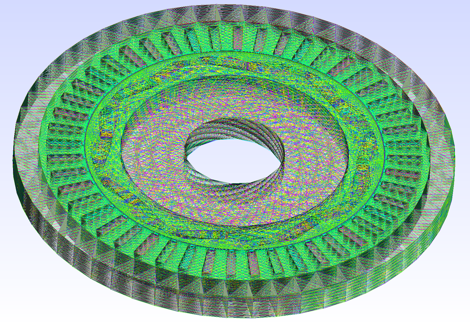
Figure 2: The space-time mesh of an 90 degrees rotating electric motor with 16 magnets and 48 coils generated by Gmsh [12]. The mesh is divided into 30 time slices in temporal direction and consists of 333 288 nodes and 1 978 689 elements.

The Galerkin space-time finite element variational formulation of (3.3) reads to find $u_{h}\in X_{h}$, such that

$$\int_{0}^{T}\int_{\Omega(t)}\left[\sigma\,\frac{d}{dt}u_{h}\,z_{h}+\nu\,\nabla_{y}u_{h}\cdot\nabla_{y}z_{h}\right]\,dy\,dt=\int_{0}^{T}\int_{\Omega(t)}\left[j_{i}\,z_{h}+M^{\perp}\cdot\nabla_{y}z_{h}\right]\,dy\,dt$$ (4.1)

is satisfied for all $z_{h}\in Y_{h}$. To ensure unique solvability of (4.1) and to derive related error estimates we proceed as in the case of a fixed domain [30]. For any $u\in X$ we define $w_{uh}\in Y_{h}$ as the unique solution of the Galerkin variational formulation

$$\int_{0}^{T}\int_{\Omega(t)}\nu\,\nabla_{y}w_{uh}\cdot\nabla_{y}z_{h}\,dy\,dt=\int_{0}^{T}\int_{\Omega(t)}\sigma\,\frac{d}{dt}u\,z_{h}\,dy\,dt\quad\mbox{for all}\;z_{h}\in Y_{h}$$ (4.2)

in order to define the discrete norm

$$\|u\|^{2}_{X_{h}}:=\|u\|^{2}_{Y}+\|w_{uh}\|^{2}_{Y}\leq\|u\|^{2}_{Y}+\|w_{u}\|^{2}_{Y}=\|u\|^{2}_{X}\quad\mbox{for all}\;u\in X.$$ (4.3)

Correspondingly, for $u_{h}\in X_{h}$ we define $w_{u_{h}h}\in Y$, and hence we can consider, due to $X_{h}\subset Y_{h}$, the particular test function $z_{h}:=u_{h}+w_{u_{h}h}\in Y_{h}$ to conclude, as in the continuous case,

$$b(u_{h},u_{h}+w_{u_{h}h})\geq\|u_{h}\|_{Y}^{2}+\|w_{u_{h}h}\|^{2}_{Y}=\|u_{h}\|^{2}_{X_{h}},\quad\|z_{h}\|_{Y}\leq\|u_{h}\|_{y}+\|w_{u_{h}h}\|_{Y}\leq\sqrt{2}\,\|u_{h}\|_{X_{h}},$$

and therefore the discrete inf-sup condition

$$\frac{1}{\sqrt{2}}\,\|u_{h}\|_{X_{h}}\leq\sup\limits_{0\neq z_{h}\in Y_{h}}\frac{b(u_{h},z_{h})}{\|z_{h}\|_{Y}}\quad\mbox{for all}\;u_{h}\in X_{h}$$ (4.4)

follows. From (4.4) we obtain unique solvability of the Galerkin variational formulation (4.1), and due to

$$\frac{1}{\sqrt{2}}\,\|u_{h}\|_{X_{h}}\leq\sup\limits_{0\neq z_{h}\in Y_{h}}\frac{b(u_{h},z_{h})}{\|z_{h}\|_{Y}}=\sup\limits_{0\neq z_{h}\in Y_{h}}\frac{b(u,z_{h})}{\|z_{h}\|_{Y}}\leq\sqrt{2}\,\|u\|_{X}$$

we conclude the boundedness of the Galerkin projection $u_{h}=G_{h}u$, i.e.,

$$\|G_{h}u\|_{X_{h}}=\|u_{h}\|_{X_{h}}\leq 2\,\|u\|_{X}\quad\mbox{for all}\;u\in X.$$

From this we further obtain

$$\|u-u_{h}\|_{X_{h}}\leq\|u-z_{h}\|_{X_{h}}+\|G_{h}(z_{h}-u)\|_{X_{h}}\leq 3\,\|u-z_{h}\|_{X}\quad\mbox{for all}\;z_{h}\in X_{h},$$

i.e., we have Cea’s lemma

$$\|u-u_{h}\|_{X_{h}}\leq 3\inf\limits_{z_{h}\in X_{h}}\|u-z_{h}\|_{X}.$$ (4.5)

When using standard finite element error estimates [5, 29] for piecewise linear approximations we finally conclude the error estimate

$$\|u-u_{h}\|_{Y}\,\leq\,c\,h\,|u|_{H^{2}(Q)}$$

when assuming $u\in H^{2}(Q)$, see [30] for the case of a fixed domain.

The Galerkin space-time finite element variational formulation (4.1) results in a huge linear system of algebraic equations, which has to be solved efficiently, and in parallel.

5 Numerical experiments

In this section we provide some numerical results in order to illustrate the applicability, the accuracy and the efficiency of the proposed approach.

We consider the electric motor as shown in Fig. 1, where both the rotor and the stator are made of laminated iron sheets, with $16$ magnets within the rotor and $48$ coils within the stator. Between the rotor and the stator there is a thin air gap, and also at the ends of the magnets air pockets are included. The material parameters for the electric conductivity $\sigma$ and the magnetic reluctivity $\nu$ for the different materials are given in Table 1. Note that the electric conductivity for iron and for the coils as given in Table 1 are chosen to be zero, since the materials in the electric motor are laminated. Moreover, we account for saturation of the ferromagnetic material, thus the reluctivity $\nu_{\text{iron}}$ in iron is a nonlinear function of the magnitude of the magnetic flux density $|B|=|\nabla u|$. Hence, the variational problem (4.1) is a nonlinear problem. The nonlinear reluctivity is computed from a spline interpolation of given discrete values for the $BH$-curve representing the relationship between magnetic flux density $B$ and magnet field strength $H$ in a ferromagnetic material. It follows from physical properties of $BH$-curves that the corresponding reluctivity function $\nu_{\text{iron}}$ satisfies a Lipschitz and strong monotonicity condition, see [24]. In the coils we are given a three-phase alternating current with an amplitude of 1555A, from which the impressed current density $j_{i}$ is obtained after dividing by the coil area. The magnetization $M$ in the permanent magnets is constant for each of the magnets and for each pair of magnets (see Fig. 1) points alternatingly inwards or outwards. The magnetization $M$ is then given by the unit vector representing a magnet’s magnetization direction multiplied with the remanence flux density $B_{R}=1.216$.

The motor is pulled up in time, where the rotation of the rotating parts, i.e., the rotor, the magnets and the air around the magnets, is already considered within the mesh for a $90$ degree rotation. As before, the time component is treated as the third spatial dimension with a time span $(0,T)$, $T=0.015$ seconds. Note that this corresponds to a rotational speed of $1000$ rotations per minute. Moreover, $30$ time slices are inserted in order to have a good temporal resolution, where the mesh is completely unstructured within the time slices, see Fig. 2. The space-time finite element mesh consists of $978689$ tetrahedral finite elements, and $333288$ nodes.

Table 1: Material parameter to desribe the electric motor.

material	$\sigma$	$\nu$
air	0	$10^{7}/(4\pi)$
coils	0	$10^{7}/(4\pi)$
magnets	$10^{6}$	$10^{7}/(4.2\pi)$
iron	0	$\nu_{\text{iron}}(|\nabla u|)$

We solve the resulting system in parallel, using a mesh decomposition method provided by the finite element library Netgen/NGSolve [27]. For our purpose, MPI parallelization is used, however the computations are done on one computer with 384 GiB RAM and two Intel Xenon Gold 5218 CPU’s with 20 cores each. For the solution of the nonlinear problem we use Newton’s method with damping where the linearized system of every Newton step is solved with GMRES supported by PETSc [6].

In a first numerical experiment, we solve a linear approximation to the nonlinear problem at hand by replacing the nonlinear magnetic reluctivity function $\nu_{\text{iron}}(|\nabla u|)$ by a constant $\nu_{1}=10^{7}/(5100\cdot 4\pi)$, which is a realistic approximation when saturation of the material does not occur. The solution to this linear problem including homogeneous initial conditions is displayed in Figure 3. Here, we made cross sections in temporal directions at specific time points. In Table 2 and Table 3 the computational times with respect to the number of cores are given for the linear problem with homogeneous initial conditions. Next we used the solution of this linearized problem as initial guess in Newton’s method for solving the nonlinear problem with the reluctivity function $\nu_{\text{iron}}=\nu_{\text{iron}}(|\nabla u|)$. The solution of the initial value problem for different points in time is depicted in Figure 4. Table 4 shows the computational time with respect to the number of cores of the Newton method stopped after 100 iterations. The initial value for the Newton method is the solution of the linear problem with zero initial conditions, as visualized in Fig. 3. Moreover, the solutions for the nonlinear problem with periodic temporal conditions are displayed in Fig. 5, but this problem was not solved in parallel.

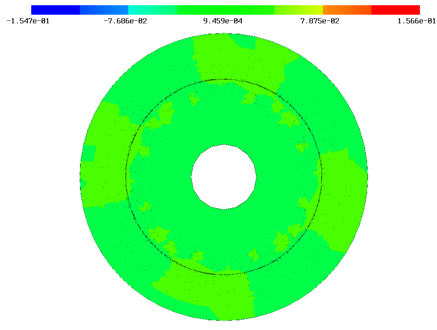
Solution at time $t=0.0$.

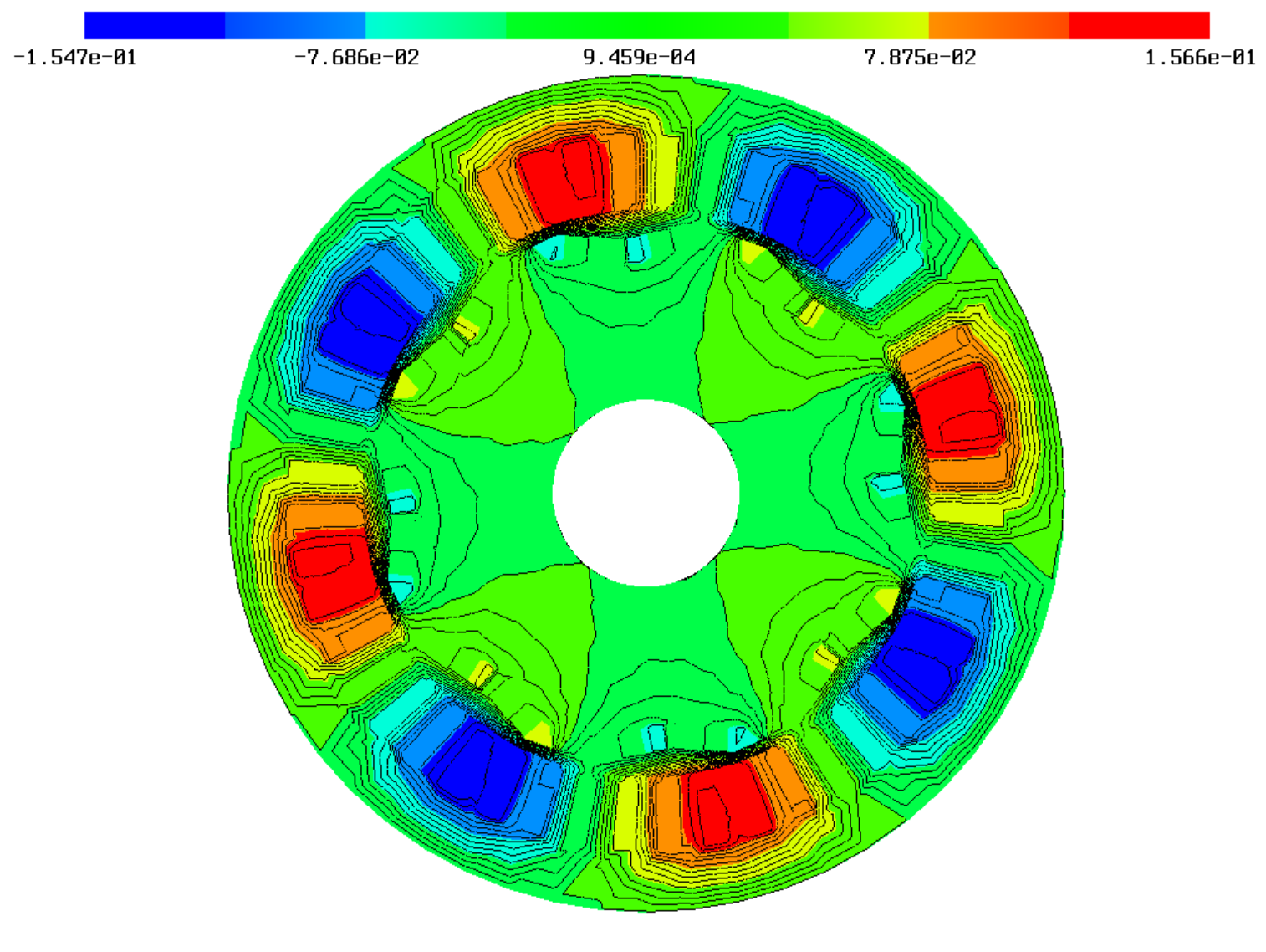
Solution at time $t=0.0045$.

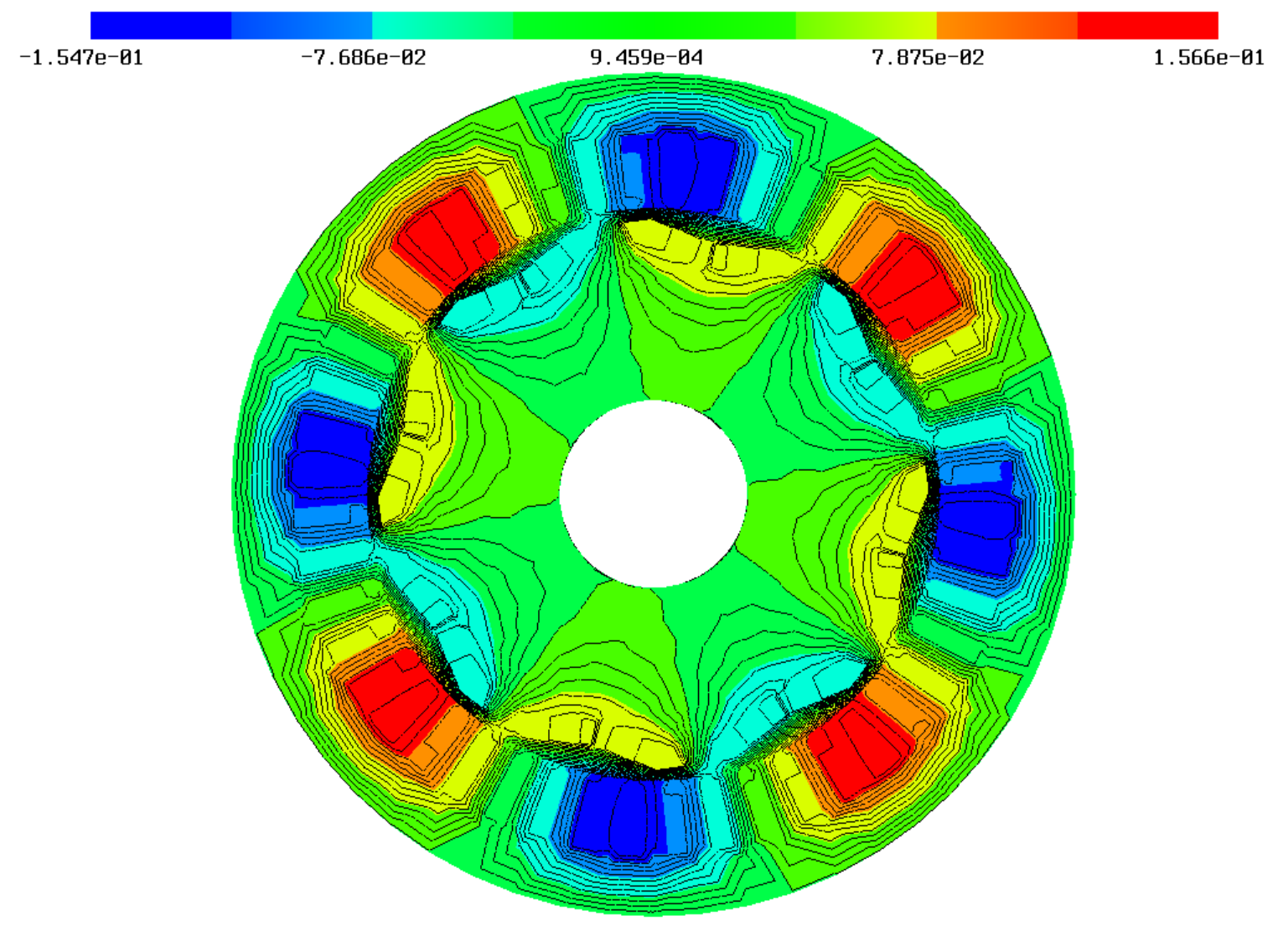
Solution at time $t=0.009$.

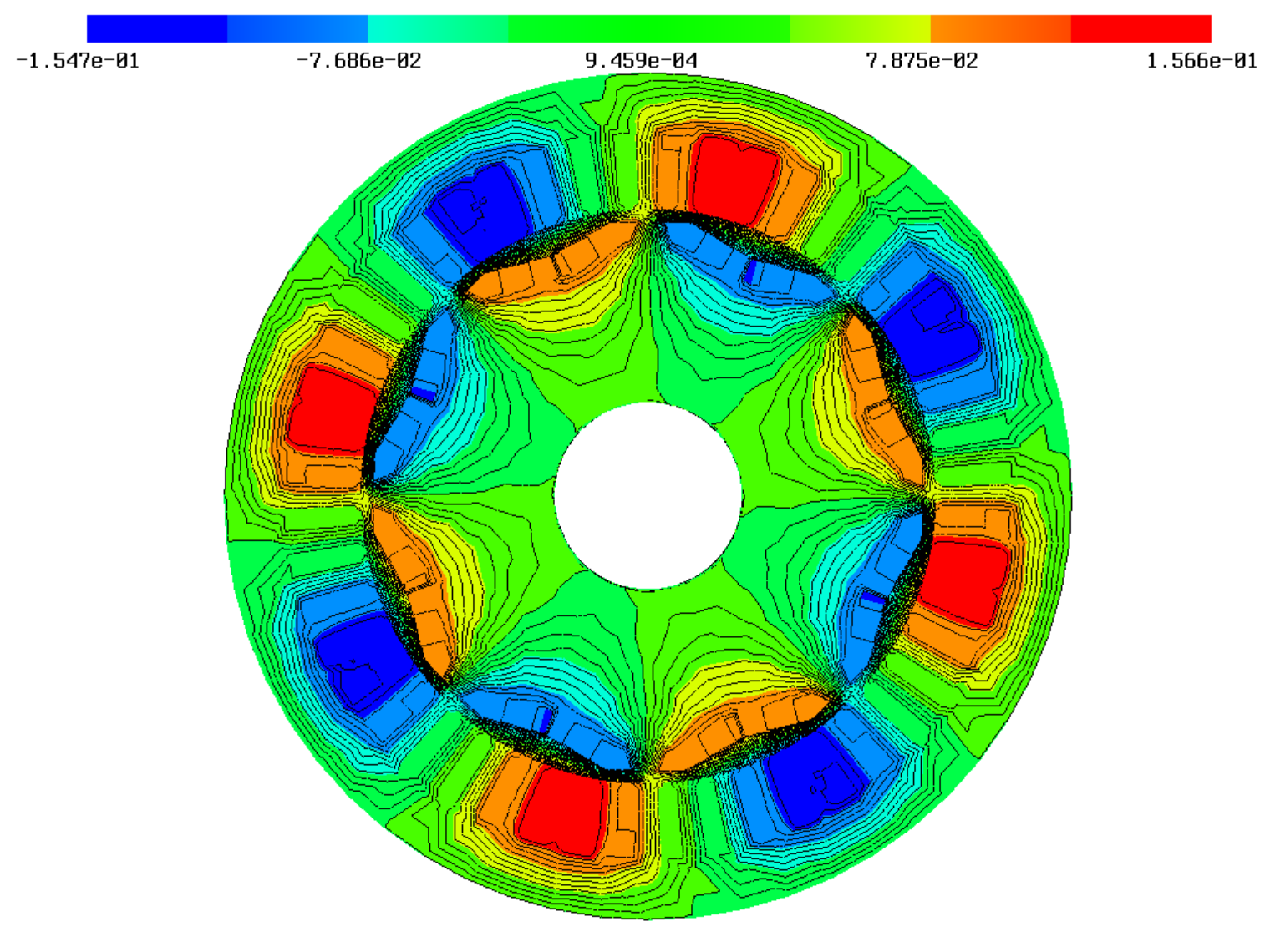
Solution at time $t=0.015$.

Figure 3: Cross sections of the solution for specific time points of the linear problem with zero initial conditions, which is considered as the start value for Newton’s method.

Table 2: Computational times in seconds of the linear problem with homogeneous initial conditions solved with MUMPS provided by PETSc [6].

number of cores	1	2	4	8	16
time in seconds	14.12	12.2	10.75	9.63	10.17

Table 3: Computational times in seconds of the linear problem with homogeneous initial conditions solved with GMRES provided by PETSc [6] up to 1000 iterations.

number of cores	1	2	4	8	16
time in seconds	16.5	11.86	7.87	4.79	3.23

Table 4: Computational times in seconds of the nonlinear problem with homogeneous initial conditions solved with GMRES with 250 iterations in every Newton iteration with a maximum of 100 Newton iterations.

number of cores	1	2	4	8	16
time in seconds	9952	5103	2761	1463	848

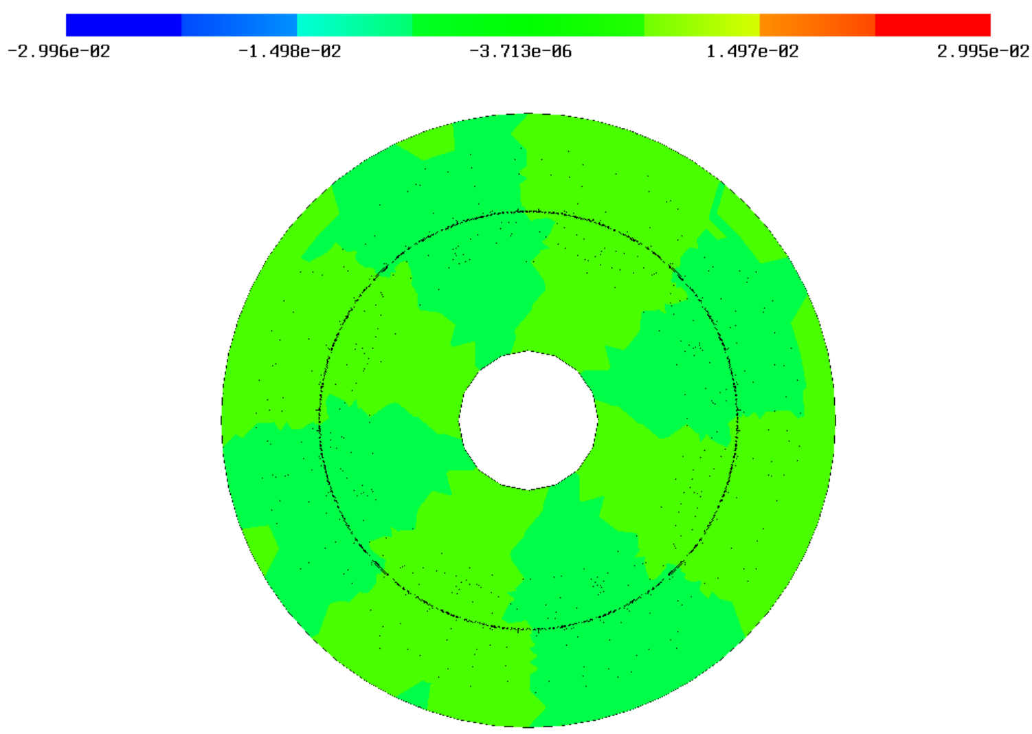
Solution at time $t=0.0$.

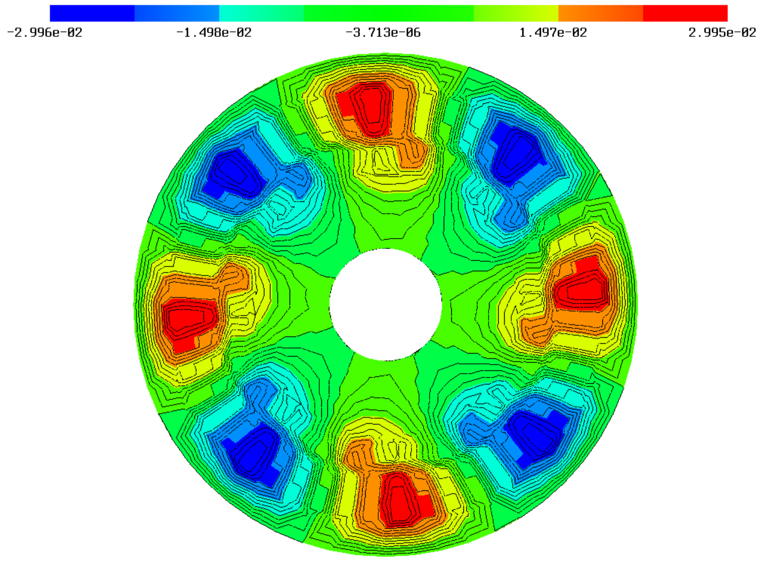
Solution at time $t=0.0045$.

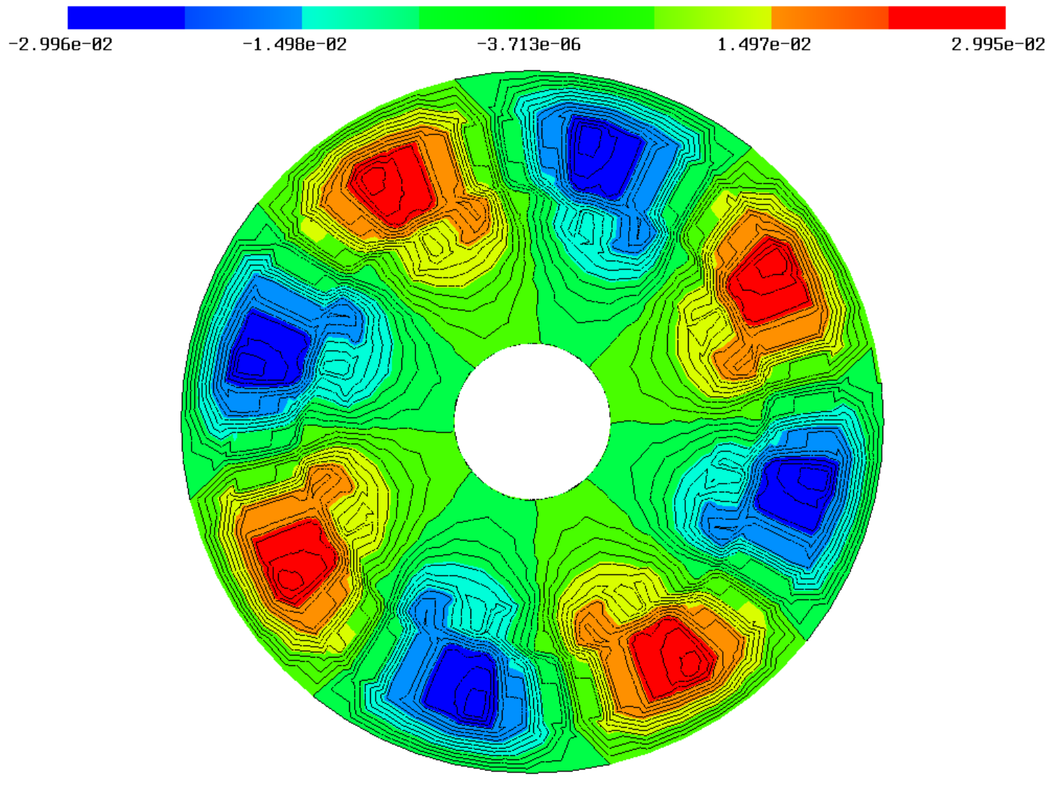
Solution at time $t=0.009$.

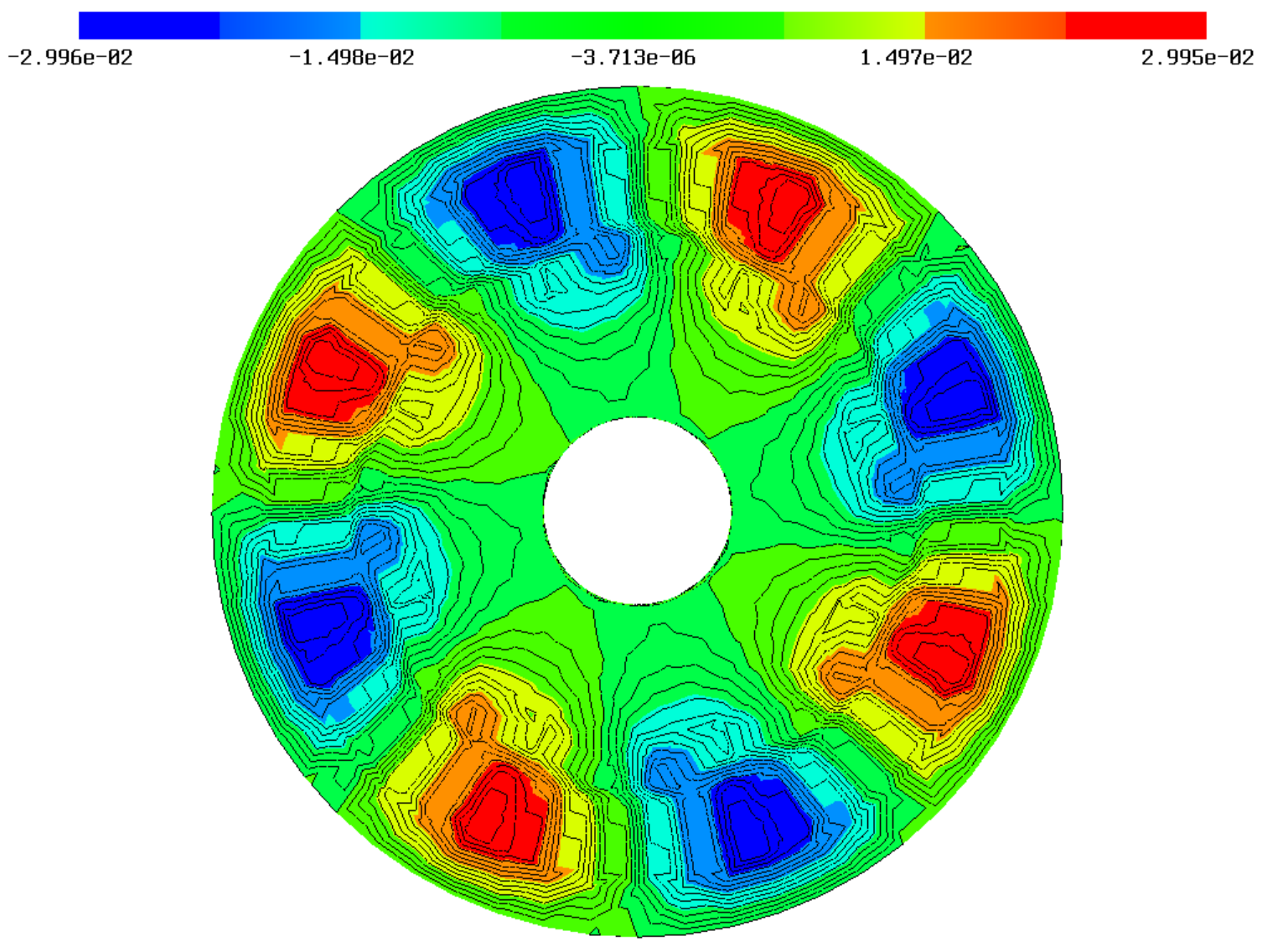
Solution at time $t=0.015$.

Figure 4: Cross sections of the solution for specific time points of the nonlinear problem with zero initial conditions.

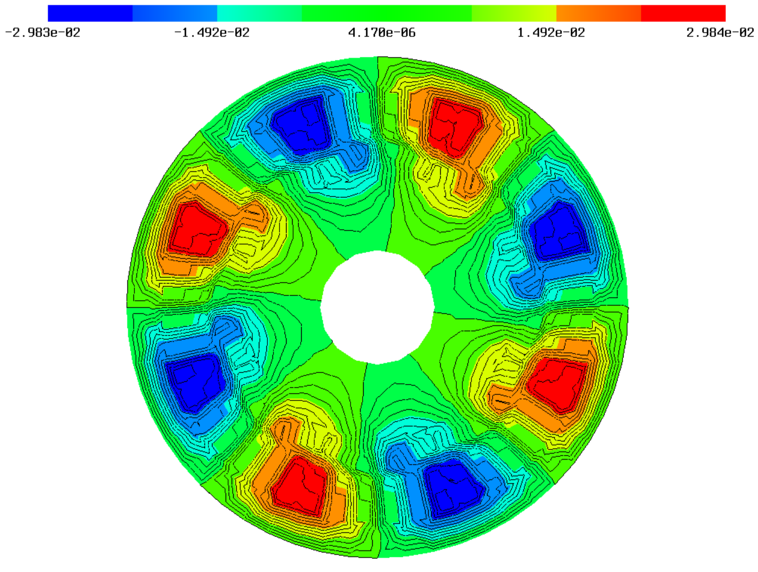
Solution at time $t=0.0$.

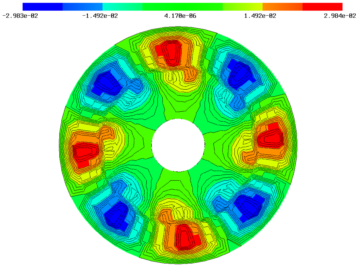
Solution at time $t=0.0045$.

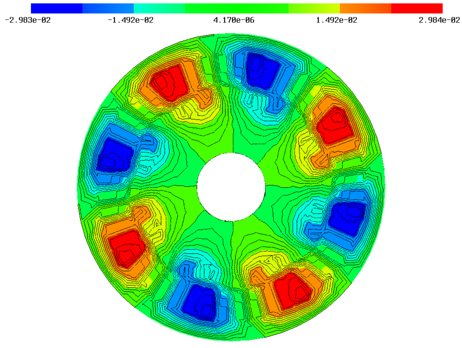
Solution at time $t=0.009$.

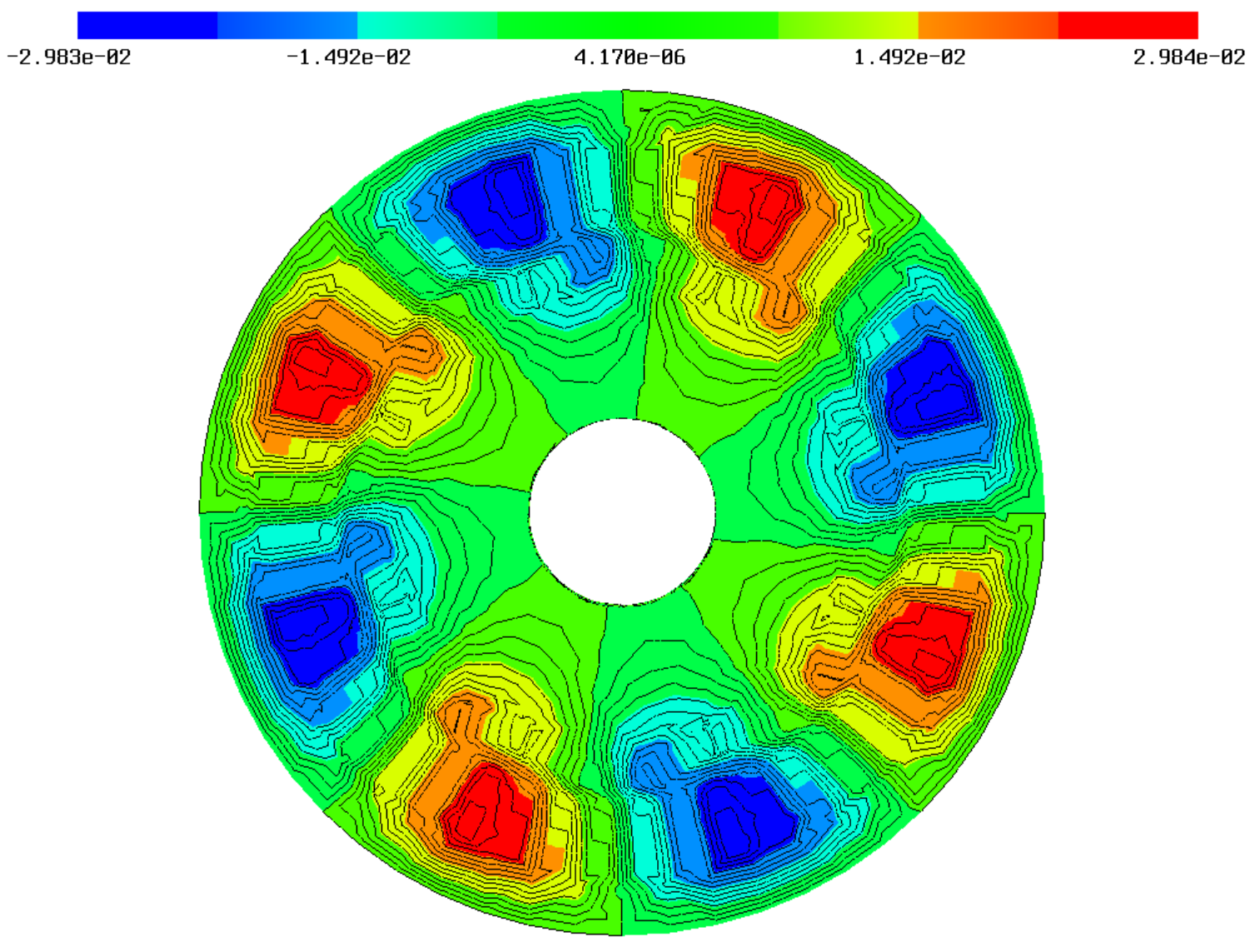
Solution at time $t=0.015$.

Figure 5: Cross sections of the solution for specific time points of the nonlinear time periodic problem.

Finally, we want to illustrate that our space-time method is also applicable to the magnetostatic problem which is obtained from (2.4) by setting $\sigma=0$ in the whole computational domain. This yields a quasi-static problem where the right hand side and the geometry are time-dependent, but no time derivative of the solution is involved. In this case, the underlying function spaces are $X=Y=L^{2}(0,T;H^{1}_{0}(\Omega(t))$ with their corresponding conforming finite dimensional subspaces $X_{h}=Y_{h}$ as described in Section 4. We consider the nonlinear reluctivity $\nu_{\text{iron}}(|\nabla u|)$ and solve the resulting system in parallel using again a damped version of Newton’s method within the FE software Netgen/NGSolve [27]. In each Newton step the linearized system is solved with GMRES or MUMPS supported by PETSc [6], where the computational times with respect to the number of cores are given in Table 5 and Table 6, respectively. The solution is visualized by making cross sections at certain time points in Fig. 6.

Table 5: Computational times in seconds of the nonlinear magnetostatic problem solved with GMRES with 250 iterations in every Newton iteration with a maximum of 100 Newton iterations.

number of cores	1	2	4	8	16
time in seconds	2979	1618	897	490	292

Table 6: Computational times in seconds of the nonlinear magnetostatic problem solved with MUMPS in every Newton iteration within 53 Newton iterations.

number of cores	1	2	4	8	16
time in seconds	2166	1374	977	733	675

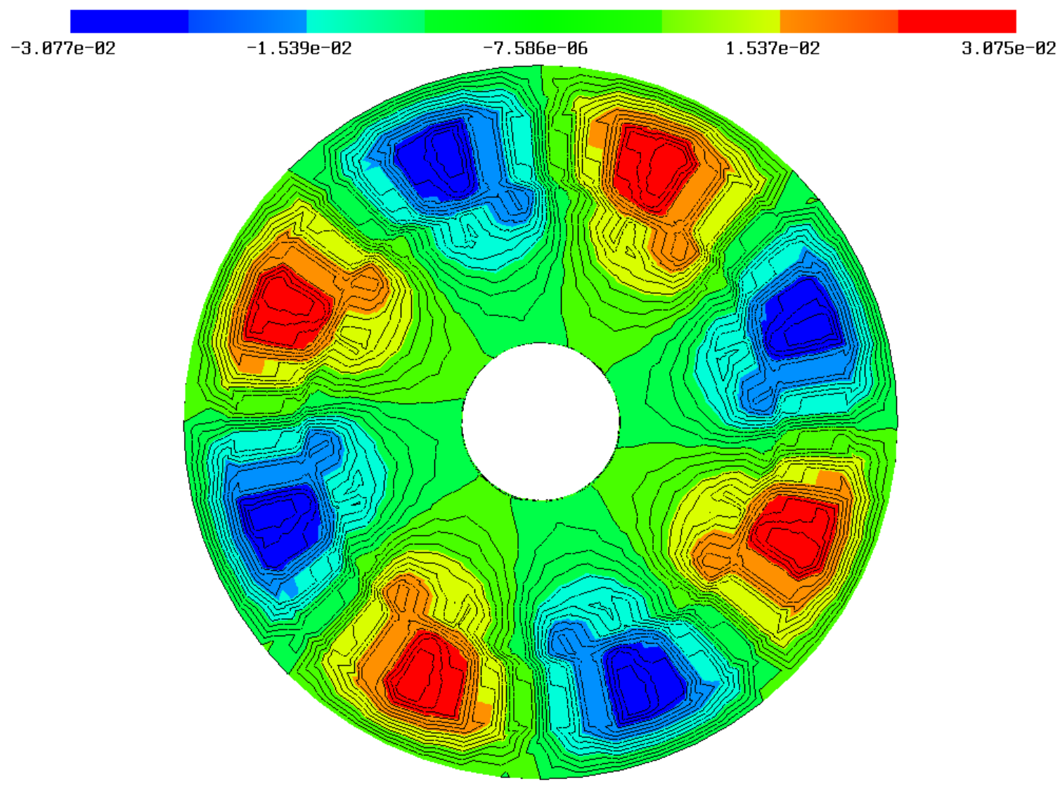
Solution at time $t=0.0$.

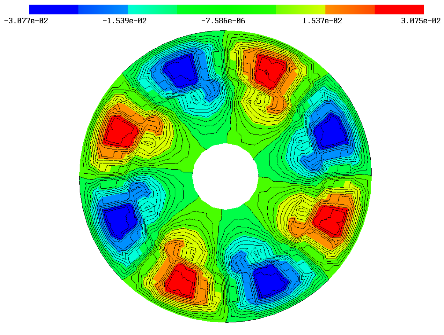
Solution at time $t=0.0045$.

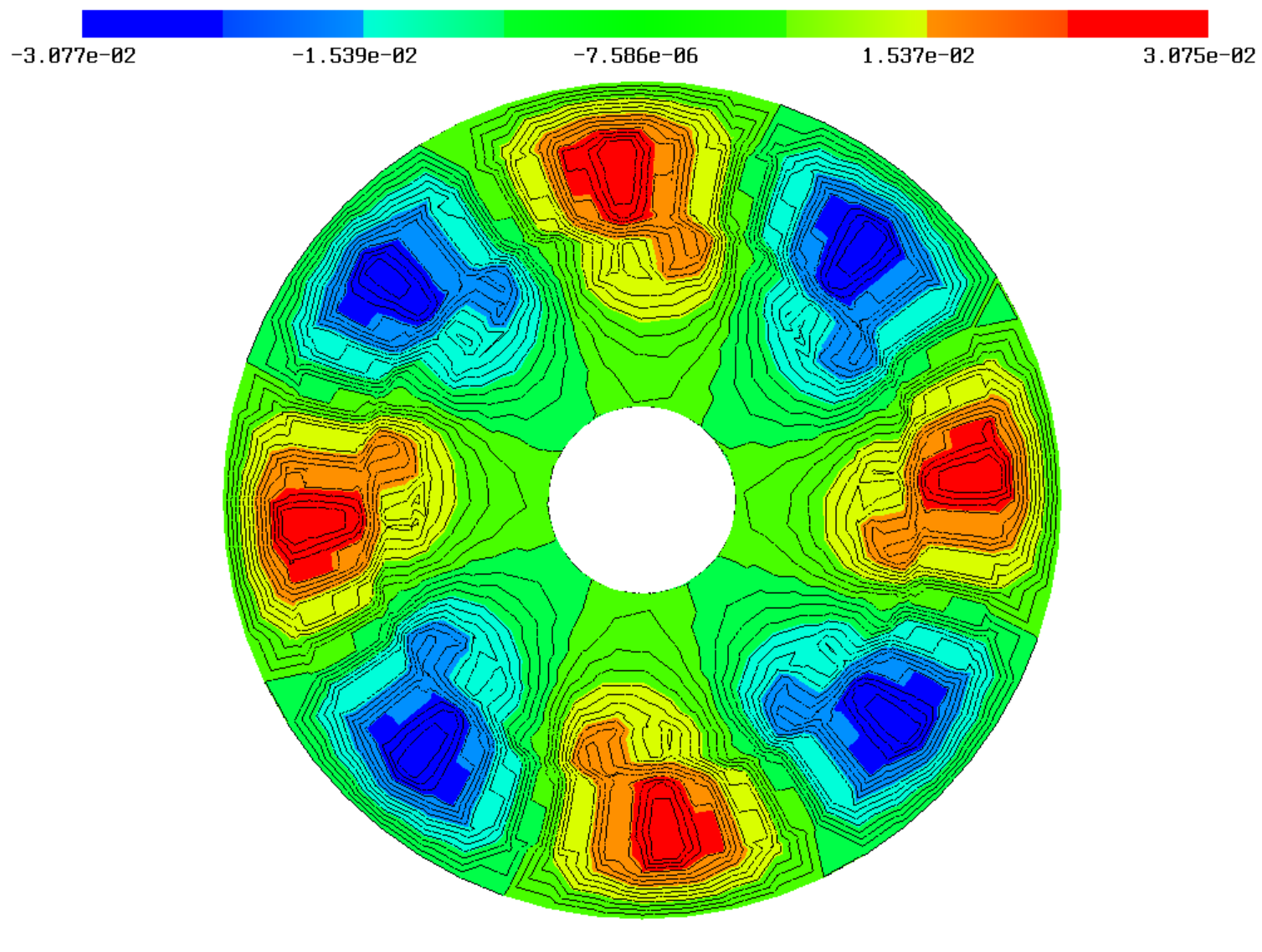
Solution at time $t=0.009$.

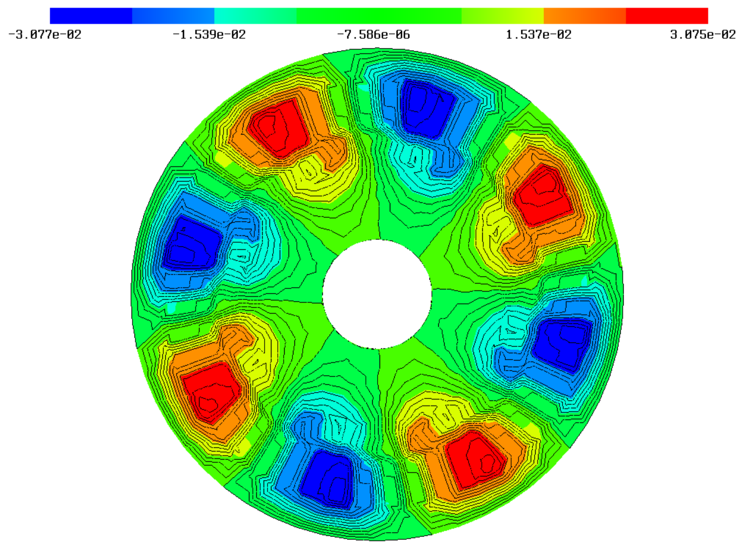
Solution at time $t=0.015$.

Figure 6: Cross sections of the solution for specific time points of the nonlinear magnetostatic problem.

6 Conclusions

In this paper we have formulated and analyzed a space-time finite element method for the numerical simulation of electromagnetic fields in rotating electric machines. As is the case of a fixed computational domain we can apply the Babuška–Nečas theory to establish unique solvability. We have presented first numerical results considering different settings for the mathematical model, including a quasi-static model, as well as a nonlinear model to describe the reluctivity. Although we have applied this approach already to an example of practical interest, it is still a challenging task to improve the parallel solver in order to handle problems with a much higher number of degrees of freedom. In addition to geometric or algebraic multigrid methods we may use space-time domain decomposition methods [31] including space-time tearing and interconnecting methods [23].

References

• [1] R. Andreev. Stability of sparse space-time finite element discretizations of linear parabolic evolution equations. IMA J. Numer. Anal., 33:242–260, 2013.
• [2] I. Babuška and A. K. Aziz. The mathematical foundations of the finite element method with applications to partial differential equations. Academic Press, New York, 1972.
• [3] F. Bachinger, U. Langer, and J. Schöberl. Numerical analysis of nonlinear multiharmonic eddy current problems. Numer. Math., 100(4):593–616, May 2005.
• [4] M. Bolten, S. Friedhoff, J. Hahne, and S. Schöps. Parallel-in-time simulation of an electrical machine using MGRIT. Comput. Visual. Sci., 23, 14, 2020.
• [5] S. C. Brenner and L. R. Scott. The mathematical theory of finite element methods, volume 15 of Texts in Applied Mathematics. Springer, New York, third edition, 2008.
• [6] L. D. Dalcin, R. R. Paz, P. A. Kler, and A. Cosimo. Parallel distributed computing using Python. Adv. Water Resour., 34:1124–1139, 2011.
• [7] A. Ern and J. Guermond. Theory and Practice of Finite Elements. Springer, New York, 2004.
• [8] S. Friedhoff, J. Hahne, I. Kulchytska-Ruchka, and S. Schöps. Exploring parallel-in-time approaches for eddy current problems. In I. Faragó, F. Izsák, and P. L. Simon, editors, Progress in Industrial Mathematics at ECMI 2018, pages 373–379, Cham, 2019. Springer.
• [9] M. Gander. 50 years of time parallel time integration, chapter Multiple shooting and time domain decomposition methods, pages 69–113. Cham: Springer, 2015.
• [10] M. J. Gander, I. Kulchytska-Ruchka, I. Niyonzima, and S. Schöps. A new parareal algorithm for problems with discontinuous sources. SIAM J. Sci. Comput., 41(2):B375–B395, 2019.
• [11] M. J. Gander and M. Neumüller. Analysis of a new space-time parallel multigrid algorithm for parabolic problems. SIAM J. Sci. Comput., 38(4):A2173–A2208, 2016.
• [12] C. Geuzaine and J.-F. Remacle. Gmsh: A three-dimensional finite element mesh generator with built-in pre- and post-processing facilities (version 2.02), 2009.
• [13] J. Gyselinck, L. Vandevelde, P. Dular, C. Geuzaine, and W. Legros. A general method for the frequency domain fe modeling of rotating electromagnetic devices. IEEE Trans. Magnet., 39(3):1147–1150, 2003.
• [14] N. Ida and J. P. A. Bastos. Electromagnetics and Calculation of Fields. Springer, New York, 1997.
• [15] I. Kulchytska-Ruchka and S. Schöps. Efficient parallel-in-time solution of time-periodic problems using a multiharmonic coarse grid correction. SIAM J. Sci. Comput., 43(1):C61–C88, 2021.
• [16] U. Langer, S. E. Moore, and M. Neumüller. Space-time isogeometric analysis of parabolic evolution problems. Comput. Methods Appl. Mech. Engrg., 306:342–363, 2016.
• [17] U. Langer, D. Pauly, and S. Repin, editors. Maxwell’s equations. Analysis and numerics, volume 24 of Radon Series on Computational and Applied Mathematics. de Gruyter, Berlin, 2019.
• [18] U. Langer and A. Schafelner. Adaptive space-time finite element methods for non-autonomous parabolic problems with distributional sources. Comput. Methods Appl. Math., 20(4):677–693, 2020.
• [19] U. Langer, O. Steinbach, F. Tröltzsch, and H. Yang. Unstructured space-time finite element methods for optimal control of parabolic equations. SIAM J. Sci. Comput., 43:A744–A771, 2021.
• [20] C. Mellak, J. Deuringer, and A. Muetze. Impact of aspect ratios of solid rotor, large air gap induction motors on run-up time and energy input. IEEE Transactions on Industry Applications, 58(5):6045–6056, 2022.
• [21] M. Neumüller and E. Karabelas. Generating admissible space-time meshes for moving domains in (d+1) dimensions. In U. Langer and O. Steinbach, editors, Space-time methods. Applications to partial differential equations, volume 25 of Radon Series on Computational and Applied Mathematics, pages 185–206. de Gruyter, Berlin, 2019.
• [22] J. Nečas. Sur une méthode pour résoudre les équations aux dérivées partielles du type elliptique, voisine de la variationnelle. Ann. Scuola Norm. Sup. Pisa, 4:305–326, 1962.
• [23] D. Pacheco and O. Steinbach. Space-time finite element tearing and interconnecting domain decomposition methods. In S. Brenner, E. Chung, A. Klawonn, F. Kwok, J. Xu, and J. Zou, editors, Domain Decomposition Methods in Science and Engineering XXVI, volume 145 of Lecture Notes in Computational Science and Engineering, pages 479–486, Cham, 2022. Springer.
• [24] C. Pechstein and B. Jüttler. Monotonicity-preserving interproximation of B–H-curves. J. Comput. Appl. Math., 196:45–57, 2006.
• [25] P. Putek. Nonlinear magnetoquasistatic interface problem in a permanent-magnet machine with stochastic partial differential equation constraints. Engineering Optimization, 51(12):2169–2192, 2019.
• [26] A. A. Rodríguez and A. Valli. Eddy Current Approximation of Maxwell Equations. Springer, Milano, 2010.
• [27] J. Schöberl. Netgen/ngsolve (version 6.2.2302), 2019.
• [28] C. Schwab and R. Stevenson. Space-time adaptive wavelet methods for parabolic evolution problems. Math. Comput., 78:1293–1318, 2009.
• [29] O. Steinbach. Numerical approximation methods for elliptic boundary value problems. Finite and boundary elements. Springer, New York, 2008.
• [30] O. Steinbach. Space-time finite element methods for parabolic problems. Comput. Methods Appl. Math., 15:551–566, 2015.
• [31] O. Steinbach and P. Gaulhofer. On space-time finite element domain decomposition methods for the heat equation. In S. Brenner, E. Chung, A. Klawonn, F. Kwok, J. Xu, and J. Zou, editors, Domain Decomposition Methods in Science and Engineering XXVI, volume 145 of Lecture Notes in Computational Science and Engineering, pages 547–554, Cham, 2022. Springer.
• [32] O. Steinbach and H. Yang. An algebraic multigrid method for an adaptive space–time finite element discretization. In I. Lirkov and S. Margenov, editors, Large-Scale Scientific Computing, pages 66–73, Cham, 2018. Springer International Publishing.
• [33] O. Steinbach and H. Yang. Space-time finite element methods for parabolic evolution equations: Discretization, a posteriori error estimation, adaptivity and solution. In U. Langer and O. Steinbach, editors, Space-time methods. Applications to partial differential equations, volume 25 of Radon Series on Computational and Applied Mathematics, pages 207–248. de Gruyter, Berlin, 2019.
• [34] O. Steinbach and M. Zank. Coercive space-time finite element methods for initial boundary value problems. Electron. Trans. Numer. Anal., 52:154–194, 2020.
• [35] R. Stevenson and J. Westerdiep. Stability of Galerkin discretizations of a mixed space-time variational formulation of parabolic evolution equations. IMA J. Numer. Anal., 41:28–47, 2021.
• [36] V. Thomée. Galerkin Finite Element Methods for Parabolic Problems. Springer, Berlin, Heidelberg, 2006.
• [37] K. Urban and A. T. Patera. An improved error bound for reduced basis approximation of linear parabolic problems. Math. Comput., 83:1599–1615, 2014.
• [38] M. Wolfmayr. A posteriori error estimation for time-periodic eddy current problems, 2023. arXiv:2305.01749.