On convergence of waveform relaxation for nonlinear systems of ordinary differential equations

Abstract

To integrate large systems of nonlinear differential equations in time, we consider a variant of nonlinear waveform relaxation (also known as dynamic iteration or Picard–Lindelöf iteration), where at each iteration a linear inhomogeneous system of differential equations has to be solved. This is done by the exponential block Krylov subspace (EBK) method. Thus, we have an inner-outer iterative method, where iterative approximations are determined over a certain time interval, with no time stepping involved. This approach has recently been shown to be efficient as a time-parallel integrator within the PARAEXP framework. In this paper, convergence behavior of this method is assessed theoretically and practically. We examine efficiency of the method by testing it on nonlinear Burgers and Liouville–Bratu–Gelfand equations and comparing its performance with that of conventional time-stepping integrators.

1 Introduction

Large systems of time-dependent ordinary differential equations arise in various applications and in many cases have to be integrated in time by implicit methods, see e.g. [1, 2]. Last decennia the niche of implicit methods has been gradually taken up by exponential time integrators [3]. For implicit and exponential methods the key issue is how to solve arising nonlinear systems and (or) to evaluate related matrix functions efficiently. To achieve efficiency, different approaches exist and widely applied, such as inexact Newton methods combined with powerful linear preconditioned solvers [4, 5, 6], splitting and Rosenbrock methods [7, 8, 9, 10, 1] and approximate iterative implicit schemes (which can be seen as stabilized explicit schemes) [11, 12, 13, 14, 15, 16, 17, 18, 19].

Another important approach to achieve efficiency in implicit and exponential time integrators is based on waveform relaxation methods [20, 21, 22], where iterative approximations are time dependent functions rather than time step values of a numerical solution. These methods have also been known as dynamic iteration or Picard–Lindelöf iteration [23]. They have been developed since the 80s [21, 24, 25, 26, 27] and have received attention recently in connection to the time-parallel exponential method PARAEXP [28] and its extension to nonlinear problems [29, 30].

Typically matrix function evaluations within exponential integrators are carried out by special linear algebra iterative procedures (often these are Krylov subspace or Chebyshev polynomial methods) [31, 32, 33, 14, 34, 35, 36]. The key attractive feature of the waveform relaxation methods is that they employ this linear algebra machinery across a certain time interval rather than within a time step, so that computational costs are distributed across time. This leads to a higher computational efficiency as well as to a parallelism across time [22].

One promising time-integration exponential method of this class is the nonlinear EBK (exponential block Krylov) method [29, 30]. It is based on block Krylov subspace projections [37] combined with waveform relaxation iteration employed to handle nonlinearities. The nonlinear EBK method possesses an across-time parallelism, and, in its parallel implementation, can be seen as an efficient version of the time-parallel PARAEXP method [29, 30].

Convergence of the waveform relaxation methods has been studied in different settings, in particular, for linear initial-value problems, for nonlinear Gauss–Seidel and Jacobi iterations (the working horses of classical waveform relaxation) and for time-discretized settings, see [23, 22] for a survey. Convergence results for waveform relaxation in general nonlinear settings are scarse, and it is often assumed that “studying the linear case carefully … might be what users really need” [23]. Except book [22], containing some general introductory convergence results, one of the papers where nonlinear waveform relaxation is studied is [38]. Below, in Remark 2, we comment more specifically on the results presented there. The aim of this paper is to extend convergence results for waveform relaxation to a nonlinear setting employed in the EBK method. This also yields an insight on its convergence behavior in practice.

The paper is organized as follows. In Section 2.1 a problem setting and the assumptions made are formulated. Main convergence results are presented in Section 2.2. Since the results are formulated for the error function which is in general unknown, in Section 2.3 an error estimate in terms of a computable nonlinear residual is formulated. At each waveform relaxation iteration a linear initial-value problem (IVP) has to be solved which, in current setting, is done by an iterative block Krylov subspace method (the linear EBK method). Therefore, in Section 2.4 we show how the nonlinear iteration convergence is affected if the linear IVP is solved inexactly. In Section 2.5 implementation issues are briefly discussed. Numerical experiments are described in Section 3.1 (for a 1D Burgers equation) and Section 3.2 (for a 3D Liouville–Bratu–Gelfand equation). We finish the paper with conclusions drawn in Section 4.

2 Nonlinear waveform relaxation and its convergence

2.1 Problem setting, assumptions and notation

We consider an IVP for nonlinear ODE system

$$y^{\prime}(t)=F(t,y(t)),\quad y(0)=v,\quad t\in[0,T]$$ (1)

where $F:\mathbb{R}\times\mathbb{R}^{N}\rightarrow\mathbb{R}^{N}$, $v\in\mathbb{R}^{N}$ and $T>0$ are given. Without loss of generality, we assume that the time dependence in the right hand side function $F$ is of the form

$$F(t,y)=\bar{F}(y)+g(t),\quad\bar{F}:\mathbb{R}^{N}\rightarrow\mathbb{R}^{N},\quad g:\mathbb{R}\rightarrow\mathbb{R}^{N}.$$ (2)

Otherwise, we can transform (1) to an equivalent autonomous form (usually this is done by extending the unknown vector function $y(t)$ with an additional $(N+1)$-th coordinate $y_{N+1}(t)=t$ and adding an ODE $y_{N+1}^{\prime}(t)=1$ to the system).

Iterative methods considered in this note are based on a family of splittings

$$F(t,y)=-A_{k}y(t)+f_{k}(y(t))+g(t),\qquad\forall\;y\in\mathbb{R}^{N},\;t\geqslant 0,$$ (3)

with $k$ being the iteration number, so that matrices $A_{k}\in\mathbb{R}^{N\times N}$ and mappings $f_{k}:\mathbb{R}^{N}\rightarrow\mathbb{R}^{N}$ may vary from iteration to iteration. The mappings $f_{k}$ in (3) are all assumed to be Lipschitz continuous with a common Lipschitz constant $L$, i.e.,

$$\forall k:\quad\|f_{k}(u)-f_{k}(v)\|\leqslant L\|u-v\|,\qquad\forall\;u,v\in\mathbb{R}^{N}.$$ (4)

Here and throughout the paper $\|\cdot\|$ denotes a vector norm in $\mathbb{C}^{N}$ or a corresponding induced matrix norm. Furthermore, we assume that for all the matrices $A_{k}$ in (3) there exist constants $C>0$ and $\omega\geqslant 0$ such that

$$\|\exp(-tA_{k})\|\leqslant Ce^{-\omega t},\qquad t\geqslant 0.$$ (5)

For a particular matrix $A=A_{k}$, condition (5) holds, for instance, in the 2-norm if the numerical range of $A$ lies in the complex halfplane $\{z=x+iy\;|\;x\geqslant 0,y\in\mathbb{R},i^{2}=-1\}$. In this case $C=1$ and $\omega$ is the smallest eigenvalue of the symmetric part $\frac{1}{2}(A+A^{T})$ of $A$. Condition (5) is closely related to the concept of the matrix logarithmic norm, see, e.g., [39, 1]. In particular, if $\mu(-A)$ is the logarithmic norm of $-A$ then condition (5) holds, with $C=1$ and for all $t\geqslant 0$, if and only if [1, Theorem I.2.4]

$$\mu(-A)\leqslant-\omega.$$

In the analysis below, we also use functions $\varphi_{j}$ [3, relation (2.10)], defined for $j=0,1,2,\dots$ as

$$\varphi_{j+1}(z)=\frac{\varphi_{j}(z)-\varphi_{j}(0)}{z},\qquad\varphi_{0}(z)=e^{z},$$ (6)

where we set $\varphi_{j}(0)=1/k!$, which makes $\varphi_{j}$ entire functions. In this paper, the following variation-of-constants formula (see, e.g., [1, Section I.2.3], [3, relation (1.5)]) is instrumental:

$$y(t)=\exp(-tA_{k})v+\int_{0}^{t}\exp(-(t-s)A_{k})\left[f_{k}(y(s))+g(s)\right]\mathrm{d}s,\quad t\in[0,T],$$ (7)

where $y(t)$ is solution of IVP (1),(3).

2.2 Nonlinear waveform relaxation

Let $y_{0}(t)$ be an approximation to the unknown function $y(t)$ for $t\in[0,T]$, with $y_{0}(0)=v$. Usually $y_{0}(t)$ is taken to be $y_{0}(t)\equiv v$ for all $t\in[0,T]$. To solve (1), in this paper we consider nonlinear waveform relaxation iteration where we solve successfully, for $k=0,1,2,\dots$, a linear inhomogeneous IVP

$$y_{k+1}^{\prime}(t)=-A_{k}y_{k+1}(t)+f_{k}(y_{k}(t))+g(t),\quad y_{k+1}(0)=v,\quad t\in[0,T].$$ (8)

Here the matrices $A_{k}\in\mathbb{R}^{N\times N}$ and the mappings $f_{k}:\mathbb{R}^{N}\rightarrow\mathbb{R}^{N}$ form a splitting of $F$, see (3), and satisfy, for all $k$, the assumptions (4),(5). We emphasize that at each iteration an approximation $y_{k+1}(t)$ is computed and stored for the whole time range $t\in[0,T]$. In Section 2.5 below we briefly discuss how to do this efficiently.

The following proposition provides a sufficient condition for iteration (8) to converge.

Proposition 1.

Let IVP (1) be solved iteratively by (8) and let assumptions (4),(5) hold for $A_{k}$ and $f_{k}$ in (8), $k=0,1,\dots$. Then for the error $\epsilon_{k+1}(t)\equiv y(t)-y_{k+1}(t)$ of the iterative approximation $y_{k+1}(t)$ holds, for $k=0,1,\dots$,

$$\|\epsilon_{k+1}(t)\|\leqslant CLt\varphi_{1}(-\omega t)\max_{s\in[0,t]}\|\epsilon_{k}(s)\|,\quad\forall t\in[0,T],$$ (9)

and nonlinear waveform relaxation (8) converges for $t\in[0,T]$ to solution $y(t)$ of IVP (1),(3) provided that

$$CLT\varphi_{1}(-\omega T)<1.$$ (10)

Proof.

For simplicity of notation throughout the proof we skip the subindeces $(\cdot)_{k}$ in the matrix $A_{k}$ and mapping $f_{k}$. Subtracting the iteration formula $y_{k+1}^{\prime}(t)=-Ay_{k+1}(t)+f(y_{k}(t))+g(t)$ from the ODE $y^{\prime}(t)=-Ay(t)+f(y(t))+g(t)$ and taking into account that $y(0)=y_{k+1}(0)=v$, we see that the error $\epsilon_{k+1}(t)$ satisfies IVP

$$\epsilon_{k+1}^{\prime}(t)=-A\epsilon_{k+1}(t)+f(y(t))-f(y_{k}(t)),\quad\epsilon_{k+1}(0)=0.$$ (11)

Then, applying the variation-of-constants formula (7) to IVP (11), we obtain

$$\epsilon_{k+1}(t)=\int_{0}^{t}\exp(-(t-s)A)\left[f(y(s))-f(y_{k}(s))\right]\mathrm{d}s.$$

Therefore, using (4) and (5), we can bound

$$\|\epsilon_{k+1}(t)\| \leqslant\int_{0}^{t}\|\exp(-(t-s)A)\|\,\|\left[f(y(s))-f(y_{k}(s))\right]\|\mathrm{d}s$$

$$\leqslant\int_{0}^{t}\|\exp(-(t-s)A)\|\,L\|y(s))-y_{k}(s)\|\mathrm{d}s$$

$$\leqslant L\max_{s\in[0,t]}\|\epsilon_{k}(s)\|\int_{0}^{t}\|\exp(-(t-s)A)\|\,\mathrm{d}s$$

$$\leqslant CL\max_{s\in[0,t]}\|\epsilon_{k}(s)\|\int_{0}^{t}e^{-\omega(t-s)}\,\mathrm{d}s=CLt\varphi_{1}(-\omega t)\max_{s\in[0,t]}\|\epsilon_{k}(s)\|.$$

Thus, (9) is proved. Taking into account that $t\varphi_{1}(-\omega t)$ is a monotonically increasing function of $t$, we obtain (10). ∎

Remark 1.

Proposition 1 shows that we can choose a length $T$ of the time interval $[0,T]$ such that the nonlinear waveform relaxation converges. The larger the Lipschitz constant $L$, the smaller $T$ should be taken.

Remark 2.

To solve an initial-value problem for an autonomous ODE system

$$C(y)y^{\prime}(t)-\bar{F}(y(t))=0,$$

in [38] a nonlinear waveform iteration

$$y^{\prime}_{k+1}(t)-\bar{F}(y_{k+1}(t))=\widehat{g}(y^{\prime}_{k}(t))$$ (12)

is considered, where $C(y)$ is a matrix and $C(y)y^{\prime}=y^{\prime}-\widehat{g}(y^{\prime})$. A convergence analysis of (12) is given in assumption that $\widehat{g}$ is Lipschitz-continuous with a Lipschitz constant less than one. In [38], a particular case of (12) is also considered with $\bar{F}(y)=-Ay+f(y)$, i.e.,

$$y^{\prime}_{k+1}(t)+Ay_{k+1}(t)-f(y_{k+1}(t))=\widehat{g}(y^{\prime}_{k}(t)).$$

Hence, our results here do not overlap with the results in [38].

In case $f(y)$ is linear, waveform relaxation (8) is known to have an attractive property to converge superlinearly for final $T$, see, e.g., [40, Theorem 5.1] and, for inexact waveform relaxation, [41, Theorem 2]. The following result shows that the superlinear convergence property is shared by nonlinear waveform relaxation (8).

Proposition 2.

Let IVP (1) be solved iteratively by (8) and let assumptions (4),(5) hold for $A_{k}$ and $f_{k}$ in (8), $k=0,1,\dots$. Then for the error $\epsilon_{k}(t)$ of the iterative approximation $y_{k}(t)$ holds, for $k=1,2,\dots$,

$$\|\epsilon_{k}(t)\| \leqslant(CL)^{k}t^{k}e^{-\omega t}\varphi_{k}(\omega t)\max_{s\in[0,t]}\|\epsilon_{0}(s)\|$$ (13)

$$\leqslant(CL)^{k}\frac{t^{k}}{k!}\max_{s\in[0,t]}\|\epsilon_{0}(s)\|,\quad\forall t\in[0,T].$$

Proof.

The proof is very similar to the proof of [40, Theorem 5.1], where a linear equivalent of (1),(8) is considered. The estimate (13) will be proven by induction. Note that $t\varphi_{1}(-\omega t)=te^{-\omega t}\varphi_{1}(\omega t)$. Therefore, the estimate (13) for $k=1$ holds, as it coincides with (9) for $k=0$. Assume that (13) holds for a certain $k$. From the proof of Proposition 1, we see that

$$\|\epsilon_{k+1}(t)\| \leqslant CL\int_{0}^{t}e^{-(t-s)\omega}\|\epsilon_{k}(s)\|\mathrm{d}s$$

and, by the induction assumption,

$$\leqslant CL\int_{0}^{t}e^{-(t-s)\omega}(CL)^{k}s^{k}e^{-\omega s}\varphi_{k}(\omega s)\max_{\tilde{s}\in[0,s]}\|\epsilon_{0}(\tilde{s})\|\mathrm{d}s$$

$$=(CL)^{k+1}e^{-\omega t}\int_{0}^{t}s^{k}\varphi_{k}(\omega s)\max_{\tilde{s}\in[0,s]}\|\epsilon_{0}(\tilde{s})\|\mathrm{d}s$$

$$\leqslant(CL)^{k+1}e^{-\omega t}\max_{s\in[0,t]}\|\epsilon_{0}(s)\|\int_{0}^{t}s^{k}\varphi_{k}(\omega s)\mathrm{d}s$$

$$=(CL)^{k+1}t^{k+1}e^{-\omega t}\varphi_{k+1}(\omega t)\max_{s\in[0,t]}\|\epsilon_{0}(s)\|,$$

where the relation $\int_{0}^{t}s^{k}\varphi_{k}(\omega s)\mathrm{d}s=t^{k+1}\varphi_{k+1}(\omega t)$ is employed. Thus, the induction step is done. Finally, using the definition of $\varphi_{k}$ and the fact that $\omega\geqslant 0$, it is not difficult to check that

$$t^{k}e^{-\omega t}\varphi_{k}(\omega t)\leqslant\frac{t^{k}}{k!},\quad t\geqslant 0,$$

which proves the second inequality in (13). ∎

2.3 Residual of the nonlinear problem

To control convergence of waveform relaxation (8) in practice, it is natural to consider a residual $r_{k}(t)$ of an iterative approximation $y_{k}(t)$ in (8). Since $y_{k}(t)$ is defined by (8),(3) written for $k-1$, it is natural to define the residual with respect to IVP (1) combined with splitting (3) for $k-1$, i.e., for IVP

$$y^{\prime}(t)=-A_{k-1}y(t)+f_{k-1}(y(t))+g(t),\quad y(0)=v,\quad t\in[0,T].$$ (14)

Hence, we define

$$r_{k}(t)\equiv-A_{k-1}y_{k}(t)+f_{k-1}(y_{k}(t))+g(t)-y_{k}^{\prime}(t),\quad t\in[0,T],$$ (15)

and write

$$r_{k}(t) =-A_{k-1}y_{k}(t)+f_{k-1}(y_{k}(t))+g(t)-y_{k}^{\prime}(t)\pm f_{k-1}(y_{k-1}(t))$$ (16)

$$=\underbrace{-A_{k-1}y_{k}(t)+f_{k-1}(y_{k-1}(t))+g(t)-y_{k}^{\prime}(t)}_{=0}+f_{k-1}(y_{k}(t))-f_{k-1}(y_{k-1}(t))$$

$$=f_{k-1}(y_{k}(t))-f_{k-1}(y_{k-1}(t)),\quad t\in[0,T],\quad k=1,2,\dots.$$

Note that the residual $r_{k}(t)$ possesses the backward error property, i.e., iterative approximation $y_{k}(t)$ can be viewed as the exact solution of a perturbed IVP (14)

$$y_{k}^{\prime}(t)=-A_{k-1}y_{k}(t)+f_{k-1}(y_{k}(t))+g(t)-r_{k}(t),\quad y_{k}(0)=v\quad t\in[0,T].$$ (17)

Subtracting the ODE of this problem from the ODE in (14), we obtain an IVP for the error $\epsilon_{k}(t)$

$$\epsilon_{k}^{\prime}(t)=-A_{k-1}\epsilon_{k}(t)+f_{k-1}(y(t))-f_{k-1}(y_{k}(t))+r_{k}(t),\quad\epsilon_{k}(0)=0,$$ (18)

which is equivalent to the IVP (11). The following proposition shows that the residual can be seen as an upper bound bound for the error.

Proposition 3.

Let IVP (1) be solved iteratively by (8) and let assumptions (4),(5) hold for $A_{k}$ and $f_{k}$ in (8), $k=0,1,\dots$. Let $T>0$ be chosen such that the sufficient condition (10) for convergence of (8) holds

$$CLT\varphi_{1}(-\omega T)\leqslant\delta<1,$$ (19)

for a certain constant $\delta\in(0,1)$. Then, for $\forall t\in[0,T]$,

$$\max_{s\in[0,t]}\|\epsilon_{k}(s)\|\leqslant\frac{Ct\varphi_{1}(-\omega t)}{1-CLt\varphi_{1}(-\omega t)}\max_{s\in[0,t]}\|r_{k}(s)\|\leqslant\frac{\delta}{(1-\delta)L}\max_{s\in[0,t]}\|r_{k}(s)\|.$$ (20)

Note that $T\varphi_{1}(-\omega T)$ increases with $T$ monotonically.

Proof.

Employing the variation-of-constants formula for IVP (18), we can bound

$$\|\epsilon_{k}(t)\| \leqslant\int_{0}^{t}\left\|\exp(-(t-s)A_{k-1})\left[f_{k-1}(y(s))-f_{k-1}(y_{k}(s))+r_{k}(s)\right]\right\|\mathrm{d}s$$

$$\leqslant\max_{s\in[0,t]}\left\|f_{k-1}(y(s))-f_{k-1}(y_{k}(s))+r_{k}(s)\right\|\int_{0}^{t}\|\exp(-(t-s)A_{k-1})\|\,\mathrm{d}s$$

$$\leqslant\max_{s\in[0,t]}\left\|f_{k-1}(y(s))-f_{k-1}(y_{k}(s))+r_{k}(s)\right\|\,Ct\varphi_{1}(-\omega t)$$

$$\leqslant\left(L\max_{s\in[0,t]}\|\epsilon_{k}(s)\|+\max_{s\in[0,t]}\|r_{k}(s)\|\right)\,Ct\varphi_{1}(-\omega t)$$

$$\leqslant CLt\varphi_{1}(-\omega t)\max_{s\in[0,t]}\|\epsilon_{k}(s)\|+Ct\varphi_{1}(-\omega t)\max_{s\in[0,t]}\|r_{k}(s)\|.$$

Taking into account that $CLt\varphi_{1}(-\omega t)\leqslant CLT\varphi_{1}(-\omega T)\leqslant\delta<1$ for $t\in[0,T]$, we obtain

$$(1-CLt\varphi_{1}(-\omega t))\max_{s\in[0,t]}\|\epsilon_{k}(s)\| \leqslant Ct\varphi_{1}(-\omega t)\max_{s\in[0,t]}\|r_{k}(s)\|$$

$$\max_{s\in[0,t]}\|\epsilon_{k}(s)\| \leqslant\frac{Ct\varphi_{1}(-\omega t)}{1-CLt\varphi_{1}(-\omega t)}\max_{s\in[0,t]}\|r_{k}(s)\|,$$

which yields (20). ∎

2.4 Linear inner iteration and its residual

In practice, the linear ODE system (8) at each waveform relaxation iteration can be solved by any suitable integrator with a certain accuracy tolerance. In the context of the time-parallel PARAEXP scheme, the nonlinear waveform relaxation appeared to be efficient for fluid dynamics problems [29, 30], with linear IVP (8) solved by the exponential block Krylov subspace (EBK) method [37]. Thus, in this setting we have an inner-outer iterative process where each nonlinear waveform relaxation iteration (8) involves an inner Krylov subspace iterative process $\tilde{y}_{k+1,\ell}(t)\rightarrow y_{k+1}(t)$, with $\ell$ being the inner iteration number. For notation simplicity we omit the dependence on the inner iteration number $\ell$ in $\tilde{y}_{k+1,\ell}(t)$ and write $\tilde{y}_{k+1}(t)$. These inner EBK iterations are controled by checking the norm of a residual defined, for $\tilde{y}_{k+1}(t)\approx y_{k+1}(t)$, as

$$\tilde{r}_{k+1}(t)\equiv-A_{k}\tilde{y}_{k+1}(t)+f_{k}(\tilde{y}_{k}(t))+g(t)-\tilde{y}^{\prime}_{k+1}(t),\quad t\in[0,T].$$ (21)

Here we assume that the previous iterative approximation $y_{k}(t)$ is also computed inexactly and therefore we replace $y_{k}(t)$ by $\tilde{y}_{k}(t)$. The inner iterations stop after a certian number $\ell$ of inner iterations as soon as the linear residual $\tilde{r}_{k+1}(t)$, defined by (21), is small enough in norm. The residual $\tilde{r}_{k+1}(t)$ turns out to be easily computable as a by-product of the block Krylov subspace method [37]. Moreover, the residual in (21) can be used as a controller for the error in the linear IVP (8), see [37, relation 16].

The following result shows that convergence in the nonlinear waveform relaxation is retained if the IVP (8) at each nonlinear iteration is solved approximately, such that residual (21) is small enough in norm, i.e., more precisely, is bounded in norm by the error achieved at a previous nonlinear iteration ((22)).

Proposition 4.

Let IVP (1) be solved iteratively by (8) and let assumptions (4),(5) hold. Furthermore, let the IVP (8) at each nonlinear iteration $k=0,1,\dots$ be solved approximately with $\ell$ inner iterations such that for the inner iteration residual (21) holds

$$\max_{s\in[0,t]}\|\tilde{r}_{k+1}(s)\|\leqslant l\max_{s\in[0,t]}\|\tilde{\epsilon}_{k}(s)\|,\quad\forall t\in[0,T],$$ (22)

where $\tilde{\epsilon}_{k}(t)\equiv y(t)-\tilde{y}_{k}(t)$ and $l>0$ is a constant. Then for the error $\tilde{\epsilon}_{k+1}(t)$ of the iterative approximation $\tilde{y}_{k+1}(t)$ holds, for $k=0,1,\dots$,

$$\|\tilde{\epsilon}_{k+1}(t)\|\leqslant C(L+l)t\varphi_{1}(-\omega t)\max_{s\in[0,t]}\|\tilde{\epsilon}_{k}(s)\|,\quad\forall t\in[0,T].$$ (23)

Hence, the inexact nonlinear waveform relaxation (8) converges for $t\in[0,T]$ to solution $y(t)$ of IVP (1),(3) provided that

$$C(L+l)T\varphi_{1}(-\omega T)<1.$$ (24)

Proof.

It follows from (21) that $\tilde{y}^{\prime}_{k+1}(t)$ solves a perturbed ODE system

$$\tilde{y}^{\prime}_{k+1}(t)=-A_{k}\tilde{y}_{k+1}(t)+f_{k}(\tilde{y}_{k}(t))+g(t)-\tilde{r}_{k+1}(t).$$

Subtracting this equation from the original nonlinear ODE $y^{\prime}(t)=-A_{k}y(t)+f_{k}(y(t))+g(t)$ and taking into account that $\tilde{y}_{k+1}(0)=y(0)=v$, we obtain an IVP for the error $\tilde{\epsilon}_{k+1}(t)\equiv y(t)-\tilde{y}_{k}(t)$ (cf. (11)):

$$\tilde{\epsilon}^{\prime}_{k+1}(t)=-A_{k}\tilde{\epsilon}_{k+1}(t)+f_{k}(y(t))-f_{k}(\tilde{y}_{k}(t))+\tilde{r}_{k+1}(t),\quad\tilde{\epsilon}_{k+1}(0)=0.$$

The rest of the proof closely follows the proof of Proposition 1. With the help of variation-of-constants formula (7), we obtain

$$\tilde{\epsilon}_{k+1}(t)=\int_{0}^{t}\exp(-(t-s)A_{k})\left[f_{k}(y(s))-f_{k}(\tilde{y}_{k}(s))+\tilde{r}_{k+1}(s)\right]\mathrm{d}s.$$

Then, using (4),(5),(22) and making the estimates similar to the proof of Proposition 1, we have

$$\|\tilde{\epsilon}_{k+1}(t)\| \leqslant\int_{0}^{t}\|\exp(-(t-s)A_{k})\|\,\|\left[f_{k}(y(s))-f_{k}(\tilde{y}_{k}(s))+\tilde{r}_{k+1}(s)\right]\|\mathrm{d}s$$

$$\leqslant Ct\varphi_{1}(-\omega t)\left[L\max_{s\in[0,t]}\|\tilde{\epsilon}_{k}(s)\|+\max_{s\in[0,t]}\|\tilde{r}_{k+1}(s)\|\right]$$

$$\leqslant Ct\varphi_{1}(-\omega t)\left[L\max_{s\in[0,t]}\|\tilde{\epsilon}_{k}(s)\|+l\max_{s\in[0,t]}\|\tilde{\epsilon}_{k}(s)\|\right],$$

which is the sought after estimate (23). Condition (24) then follows from the observation that $t\varphi_{1}(-\omega t)$ is a monotonically increasing function of $t$. ∎

Remark 3.

Since the error $\tilde{\epsilon}_{k}(t)$ is unknown, in practice condition (22) can be replaced by requirement that $\|\tilde{r}_{k+1}(t)\|$ is small with respect to the nonlinear residual norm $\|r_{k}(t)\|$, cf. (20).

2.5 Implementation of nonlinear waveform relaxation

We take initial guess function $y_{0}(t)$ identically (i.e., for all $t\in[0,T]$) equal to the initial vector $y_{0}(t)\equiv v$. Then, at each iteration (8) we set $\tilde{g}(t):=f_{k}(y_{k}(t))+g(t)$ and solve a linear IVP

$$y^{\prime}_{k+1}(t)=-A_{k}y_{k+1}(t)+\tilde{g}(t),\quad y_{k+1}(0)=v,\quad t\in[0,T].$$ (25)

Since this IVP is solved by the EBK method [37], the solution $y_{k+1}(t)$ at every iteration is obtained as a linear combination of Krylov subspace vectors, where the coefficients of this combination are solution of a small-sized projected IVP. This allows to store $y_{k+1}(t)$ in a compact way for all $t\in[0,T]$. At each nonlinear iteration $k$ the EBK method stops as soon as the residual (21) is small enough in norm. The residual norm is easily computable and is checked for several values of $t\in[0,T]$.

Starting with the second iteration $k=1$, before the IVP (25) is solved, the vector function $\tilde{g}(y_{k}(t))$ is sampled at $s$ points $t_{!}$, …, $t_{s}$ covering the time interval $[0,T]$. Usually, it is sensible to take $t_{1}=0$, $t_{s}=T$ and the other $t_{j}$ to be the Chebyshev polynomial roots:

$$t_{j}=\frac{T}{2}\left(1-\cos\frac{\pi(j-3/2)}{s-2}\right),\quad j=2,\dots,s-1.$$

The number of sample points $s$ should be taken such that $\tilde{g}(y_{k}(t))$ is sufficiently well approximated by its linear interpolation at $t_{1}$, …, $t_{s}$. The computed samples $\tilde{g}(t_{j})=\tilde{g}(y_{k}(t_{j}))$, $j=1,\dots,s$, are then stored as the columns of a matrix $\tilde{G}\in\mathbb{R}^{n\times s}$ and the thin singular value decomposition of $\tilde{G}$ is employed to obtain a low rank representation

$$\tilde{g}(t)\approx Up(t),\quad U\in\mathbb{R}^{n\times m},\quad t\in[0,T],$$ (26)

where typically $m<10$. For more details of this procedure we refer to [37] or to [29]. Usually the computational work needed to obtain representation $\tilde{g}(t)\approx Up(t)$ is negligible with respect to the other work in the EBK method. The nonlinear iteration (8) is stopped as soon as the nonlinear residual (16) is small enough in norm (in our limited experience, in practice it suffice to check the residual norm at final time $t=T$ only).

3 Numerical experiments

3.1 1D Burgers equation

This IVP is taken from [42, Ch. IV.10]. To find unknown function $u(x,t)$, we solve a 1D Burgers equation

$$u_{t}=\nu u_{xx}-uu_{x},\quad 0\leqslant x\leqslant 1,\quad 0\leqslant t\leqslant T,$$

with viscosity $\nu=3\cdot 10^{-4}$ and $\nu=3\cdot 10^{-5}$. Initial and boundary conditions are

$$u(x,0)=\frac{3}{2}x(1-x)^{2},\quad u(0,t)=u(1,t)=0,$$

and the final time $T$ is set to $0.5$, $1.0$, and $1.5$. We discretize the Burgers equation by finite differences on a uniform mesh with $n$ internal nodes $x_{j}=j\Delta x$, $j=1,\dots,n$, $\Delta x=1/(n+1)$. To avoid numerical energy dissipation and to guarantee that a discretization of the advection term $uu_{x}$ results in a skew-symmetric matrix [43], we apply the standard second-order central differences in the following way

$$uu_{x}=\frac{1}{3}uu_{x}+\frac{2}{3}\left(\frac{u^{2}}{2}\right)_{x}\approx\frac{1}{3}u_{i}\frac{u_{i+1}-u_{i-1}}{2\Delta x}+\frac{2}{3}\frac{u_{i+1}^{2}-u_{i-1}^{2}}{4\Delta x}.$$

The diffusion term $\nu u_{xx}$ is discretized by second-order central differences in the usual way. Then this finite difference discretization leads to an IVP of the form

$$y^{\prime}(t)=-A_{\mathrm{symm}}y(t)-A_{\mathrm{skew}}(y(t))y(t),\quad y(0)=v,$$ (27)

where

$$A_{\mathrm{symm}}y\approx-\nu u_{xx},\quad A_{\mathrm{skew}}(y)y\approx uu_{x},$$

$A_{\mathrm{symm}}=A_{\mathrm{symm}}^{T}$ is positive definite and $(A_{\mathrm{skew}}(y))^{T}=-A_{\mathrm{skew}}(y)$ for all $y\in\mathbb{R}^{N}$. A straightforward way to apply the nonlinear iteration (8) to (27) would be setting in (3) $A_{k}:=A_{\mathrm{symm}}$, $f_{k}(y):=-A_{\mathrm{skew}}(y)y$. However, to decrease the Lipschitz constant of $f_{k}(y)$ (cf. condition (10)), we also include a linear part of $-A_{\mathrm{skew}}(y)y$ to the $-A_{k}y$ term in (3). More specifically, we apply the nonlinear iteration (8) to semidiscrete Burgers equation (27) in the form

$$y_{k+1}^{\prime}(t)=-(\,\underbrace{A_{\mathrm{symm}}+A_{\mathrm{skew}}(\bar{y}_{k})}_{\displaystyle A_{k}}\,)y_{k+1}(t)+\underbrace{\left[A_{\mathrm{skew}}(\bar{y}_{k})-A_{\mathrm{skew}}(y_{k}(t))\right]y_{k}(t)}_{\displaystyle f_{k}(y_{k}(t))},$$ (28)

$$k=0,1,2,\dots,$$

where $\bar{y}_{k}=y_{k}(T)$. The nonlinear residual (16) in this case reads, for $k=0,1,\dots$,

$$r_{k+1}(t) =f_{k}(y_{k+1}(t))-f_{k}(y_{k}(t))$$

$$=\left[A_{\mathrm{skew}}(\bar{y}_{k})-A_{\mathrm{skew}}(y_{k+1}(t))\right]y_{k+1}(t)-\left[A_{\mathrm{skew}}(\bar{y}_{k})-A_{\mathrm{skew}}(y_{k}(t))\right]y_{k}(t),$$

$$r_{k+1}(T) =\left[A_{\mathrm{skew}}(\bar{y}_{k})-A_{\mathrm{skew}}(y_{k+1}(T))\right]y_{k+1}(T).$$

We stop our nonlinear iterative process (8) as soon as

$$\|r_{k}(T)\|\leqslant\texttt{tol},$$

where tol is a tolerance value. As we primarily aim at solving IVPs stemming from space discretization of PDEs, where space discretization error is significant, we settle for a moderate tolerance value $\texttt{tol}=10^{-3}$ in this test. To obtain the low rank representation (26) at each iteration $k$ we use $s=100$ sample points $t_{j}$, $j=1,\dots,s$ and set the number $m$ of singular vectors to $m=7$. The largest truncated singular value $\sigma_{m+1}$, serving as an indicator of the relative low rank representation error in (26), is then of order $10^{-6}$ for $T=0.5$ and of order $10^{-3}$ for $T=1.5$.

For the inner iterative solver EBK employed to solve (8) we set the residual tolerance to $\texttt{tol}_{\mathtt{EBK}}=\texttt{tol}$ and Krylov subspace dimension to $10$. As the block size in the Krylov subspace process is $m=7$, the EBK solver requires $m(10+1)=77$ vectors to store. Since the problem becomes stiffer as the spatial grid gets finer, we use the EBK solver in the shift-and-invert (SAI) mode [44], i.e., the block Krylov subspace is computed for the SAI matrix $(I+\gamma A_{k})^{-1}$, $\gamma=T/10$, with $A_{k}$ defined in (28). A sparse (banded in this test) LU factorization of $I+\gamma A_{k}$ is computed once at each nonlinear iteration and used every time an action of $(I+\gamma A_{k})^{-1}$ is required.

To compare our nonlinear iterative EBK solver to another solver, we also solve this test with a MATLAB stiff ODE solver ode15s. This is a variable step szie and variable order implicit multistep method [45]. The ode15s solver is run with absolute and relative tolerances set, respectively, to $\texttt{AbsTol}=\texttt{tol}$ and $\texttt{RelTol}=10^{4}\texttt{tol}$, with $\texttt{tol}=10^{-9}$. For these tolerance values both ode15s and our nonlinear EBK deliver a comparable accuracy. The relative error values reported below are computed as

$$\frac{\|y-y_{\mathrm{ref}}\|}{\|y_{\mathrm{ref}}\|},$$ (29)

where $y$ is a numerical solution at final time $T$ and $y_{\mathrm{ref}}$ is a reference solution computed at final time by the ode15s solver run with strict tolerance values $\texttt{AbsTol}=10^{-12}$ and $\texttt{RelTol}=10^{-8}$. As $y_{\mathrm{ref}}$ is computed on the same spatial grid as $y$, the error value can be seen as a reliable measure of time accuracy [13].

Actual delivered accuracies and corresponding required computational work for both solvers are reported in Table 1 (for viscosity $\nu=3\cdot 10^{-4}$) and Table 2 (for $\nu=3\cdot 10^{-5}$). For our nonlinear EBK solver the work is reported as the number of nonlinear iterations, with one LU factorization and one matrix-vector product (matvec) per iteration, and the total number of linear systems solutions (which equals the total number of Krylov steps times the block size $m$). The reported total number of LU applications is not necessarily a multiple of the block size $m=7$ because at the first nonlinear iteration the approximate solution is constant in time and, hence, we set $m=1$ in (26) at the first iteration. The computational work for the ode15s solver is reported as the number of time steps, computed LU factorizations and the ODE right hand side function evaluations (fevals).

Table 1: The 1D Burgers test problem, viscosity $\nu=3\cdot 10^{-4}$. Attained error and computational work for our nonlinear EBK method and the ode15s solver. For the EBK method the work is reported as the nonlinear iteration number, number of LU factorizations, their applications and matvecs. For the ode15s solver the work is measured the as the number of time steps, LU factorizations, their applications and fevals.

	method,	iter./	LUs (LUs applic.),	relative
$T$	tolerance	steps	matvecs/fevals	error
grid $n=500$, $\|A_{\mathrm{symm}}+A_{\mathrm{skew}}(y(T))\|_{1}\approx 300$
$0.5$	nonlin.EBK($m=7$), 1e-03	5	5 (141), 5	5.17e-06
$1.0$	nonlin.EBK($m=7$), 1e-03	7	7 (220), 7	2.03e-05
$1.5$	nonlin.EBK($m=7$), 1e-03	10	10 (340), 10	5.31e-05
$0.5$	ode15s, 1e-09	59	14 (73), 575	1.93e-06
$1.0$	ode15s, 1e-09	70	16 (86), 588	8.38e-06
$1.5$	ode15s, 1e-09	83	19 (118), 620	2.21e-05
grid $n=1000$, $\|A_{\mathrm{symm}}+A_{\mathrm{skew}}(y(T))\|_{1}\approx 1\,200$
$0.5$	nonlin.EBK($m=7$), 1e-03	5	5 (170), 5	5.06e-06
$1.0$	nonlin.EBK($m=7$), 1e-03	7	7 (256), 7	2.00e-05
$1.5$	nonlin.EBK($m=7$), 1e-03	10	10 (389), 10	5.30e-05
$0.5$	ode15s, 1e-09	67	15 (83), 1085	1.76e-06
$1.0$	ode15s, 1e-09	78	17 (104), 1106	1.13e-05
$1.5$	ode15s, 1e-09	91	19 (134), 1136	2.48e-05
grid $n=2000$, $\|A_{\mathrm{symm}}+A_{\mathrm{skew}}(y(T))\|_{1}\approx 4\,800$
$0.5$	nonlin.EBK($m=7$), 1e-03	5	5 (177), 5	5.07e-06
$1.0$	nonlin.EBK($m=7$), 1e-03	7	7 (277), 7	2.00e-05
$1.5$	nonlin.EBK($m=7$), 1e-03	11	11 (452), 11	4.38e-05
$0.5$	ode15s, 1e-09	73	16 (91), 2093	2.29e-06
$1.0$	ode15s, 1e-09	85	19 (107), 2109	7.96e-06
$1.5$	ode15s, 1e-09	98	22 (139), 2141	2.22e-05
grid $n=4000$, $\|A_{\mathrm{symm}}+A_{\mathrm{skew}}(y(T))\|_{1}\approx 19\,200$
$0.5$	nonlin.EBK($m=7$), 1e-03	5	5 (193), 5	5.06e-06
$1.0$	nonlin.EBK($m=7$), 1e-03	8	8 (347), 8	4.82e-06
$1.5$	nonlin.EBK($m=7$), 1e-03	11	11 (501), 11	4.38e-05
$0.5$	ode15s, 1e-09	79	18 (99), 4101	1.93e-06
$1.0$	ode15s, 1e-09	90	20 (112), 4114	8.25e-06
$1.5$	ode15s, 1e-09	103	23 (144), 4146	2.21e-05

As we can see in Tables 1 and 2, our solver requires less LU factorizations than the ode15s solver. It does require more LU factorization actions but these are relatively cheap. Moreover, in EBK they are carried out simultaneously for blocks of $m$ right hand sides. For both solvers, in Figure 1 we plot the numbers of LU factorizations (presented in the tables) versus the grid size. The number of nonlinear iterations in the EBK solver (with one LU factorization per iteration) remains practically constant as the grid gets finer, whereas the number of LU factorizations in ode15s increases with the grid size. Furthermore, we see that the ode15s solver requires more time steps and significantly more fevals on the finer grids, which is not the case for our solver. $T=1.5$ is approximately the largest possible time for which our nonlinear EBK solver converges in this test. From Figure 1 we see that a higher efficiency is reached for larger $T$ values. Indeed, on the finest grid $n=4000$ $5\times 2=10$ LU factorizations per unit time are required for $T=0.5$, $8$ LU factorizations for $T=1$ and $11/1.5\approx 7$ factorizations for $T=1.5$.

Comparing Tables 1 and 2, we see that performance of the ode15s solver improves for the smaller viscosity value $\nu=3\cdot 10^{-5}$. This is expected as the stiffness of the space-discretized Burgers equation decreases with $\nu$. Indeed, on finer grids, where contributions of $A_{\mathrm{symm}}$ (proportional to $(\Delta x)^{-2}$) dominate those of $A_{\mathrm{skew}}(t)$ (proportional to $(\Delta x)^{-1}$), we have $\|A_{\mathrm{symm}}+A_{\mathrm{skew}}(t)\|\approx\mathcal{O}(\nu)$, see the values $\|A_{\mathrm{symm}}+A_{\mathrm{skew}}(T)\|$ reported in the tables.

In Figure 2 we plot the reference solution $y_{\mathrm{ref}}(T)$ and the first three iterative apporximations $y_{0}(T)=v$, $y_{1}(T)$ and $y_{2}(T)$. Convergence plots of the residual and error norms are shown in Figure 3. There, the shown residual norm is computed at $t=T$ according to (16) and the error norm is the relative norm defined in (29). As we see, the residual turns out to be a reliable measure of the error. Furthermore, convergence behavior is not influenced by viscosity $\nu$, which is in accordance with theory: $\nu$ does not change the nonlinear term $f_{k}$ in (8) and its Lipschitz constant.

Table 2: The 1D Burgers test problem, viscosity $\nu=3\cdot 10^{-5}$. Attained error and computational work for our nonlinear EBK method and the ode15s solver. For the EBK method the work is reported as the nonlinear iteration number, number of LU factorizations, their applications and matvecs. For the ode15s solver the work is measured the as the number of time steps, LU factorizations, their applications and fevals.

	method,	iter./	LUs (LUs applic.),	relative
$T$	tolerance	steps	matvecs/fevals	error
grid $n=500$, $\|A_{\mathrm{symm}}+A_{\mathrm{skew}}(y(T))\|_{1}\approx 90$
$0.5$	nonlin.EBK($m=7$), 1e-03	5	5 (69), 5	1.82e-05
$1.0$	nonlin.EBK($m=7$), 1e-03	7	7 (139), 7	2.26e-05
$1.5$	nonlin.EBK($m=7$), 1e-03	13	13 (414), 13	1.10e-04
$0.5$	ode15s, 1e-09	28	7 (38), 540	3.71e-06
$1.0$	ode15s, 1e-09	38	9 (53), 555	1.23e-05
$1.5$	ode15s, 1e-09	52	13 (89), 591	3.38e-05
grid $n=1000$, $\|A_{\mathrm{symm}}+A_{\mathrm{skew}}(y(T))\|_{1}\approx 210$
$0.5$	nonlin.EBK($m=7$), 1e-03	5	5 (90), 5	6.20e-06
$1.0$	nonlin.EBK($m=7$), 1e-03	7	7 (176), 7	2.25e-05
$1.5$	nonlin.EBK($m=7$), 1e-03	12	12 (430), 12	1.07e-04
$0.5$	ode15s, 1e-09	35	9 (44), 1046	2.44e-06
$1.0$	ode15s, 1e-09	45	10 (60), 1062	1.64e-05
$1.5$	ode15s, 1e-09	59	15 (99), 2102	3.83e-05
grid $n=2000$, $\|A_{\mathrm{symm}}+A_{\mathrm{skew}}(y(T))\|_{1}\approx 540$
$0.5$	nonlin.EBK($m=7$), 1e-03	5	5 (120), 5	5.29e-06
$1.0$	nonlin.EBK($m=7$), 1e-03	7	7 (190), 7	2.22e-05
$1.5$	nonlin.EBK($m=7$), 1e-03	12	12 (494), 12	1.06e-04
$0.5$	ode15s, 1e-09	42	10 (55), 2057	3.91e-06
$1.0$	ode15s, 1e-09	52	12 (70), 2072	1.32e-05
$1.5$	ode15s, 1e-09	66	17 (108), 4111	3.32e-05
grid $n=4000$, $\|A_{0}+A_{\mathrm{skew}}(y(T))\|_{1}\approx 1\,920$
$0.5$	nonlin.EBK($m=7$), 1e-03	5	5 (149), 5	5.24e-06
$1.0$	nonlin.EBK($m=7$), 1e-03	8	8 (276), 8	5.52e-06
$1.5$	nonlin.EBK($m=7$), 1e-03	12	12 (578), 12	1.07e-04
$0.5$	ode15s, 1e-09	47	11 (61), 4063	3.86e-06
$1.0$	ode15s, 1e-09	58	15 (80), 4082	1.22e-05
$1.5$	ode15s, 1e-09	71	18 (112), 8115	3.36e-05

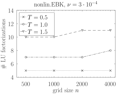
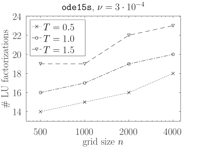
Figure 1: The Burgers test. Number of required LU factorizations versus the grid size in the nonlinear EBK solver (left) and ode15s (right) for different final time values $T$ and viscosity $\nu=3\cdot 10^{-4}$

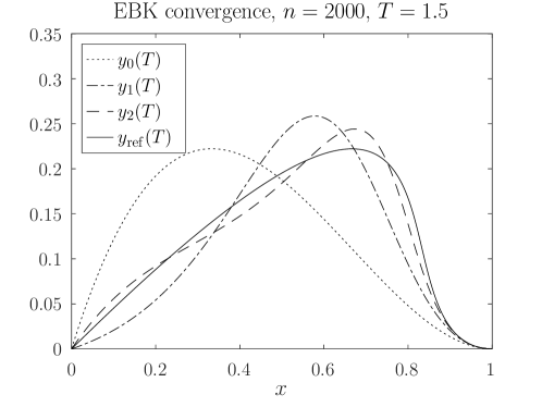
Figure 2: The Burgers test. The first three iterative apporximations $y_{0}(T)=v$, $y_{1}(T)$, $y_{2}(T)$ and reference solution $y_{\mathrm{ref}}(T)$ for the Burgers test, grid size $n=2000$, final time $T=1.5$, viscosity $\nu=3\cdot 10^{-4}$

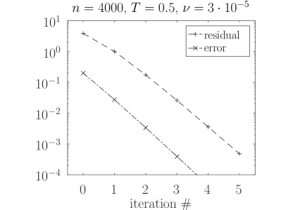
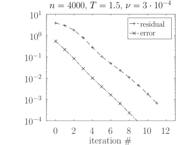
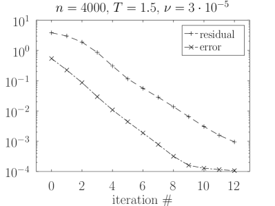
Figure 3: The Burgers test. Residual norm (16) and relative error norm (29) versus iteration number for $T=0.5$ (top plots) and $T=1.5$ (bottom plots), $\nu=3\cdot 10^{-4}$ (left plots) and $\nu=3\cdot 10^{-5}$ (right plots). The grid size is $n=4000$. Error stagnation visible at the bottom right plot can be repaired by slightly increasing the block size $m$.

3.2 3D Bratu test problem

We now consider a nonstationary IVP for Liouville–Bratu–Gelfand equation [46]: find $u=u(x,y,z,t)$ such that

$$u_{t}=10^{4}u_{xx}+10^{2}u_{yy}+u_{zz}+Ce^{u}+\tilde{g}(x,y,z,t),$$ (30)

$$\qquad\qquad(x,y,z)\in\Omega=[0,1]^{3},\quad 0\leqslant t\leqslant T,\quad C=3\cdot 10^{4},$$

$$u(x,y,z,0)=e^{-100\left((x-0.2)^{2}+(y-0.4)^{2}+(z-0.5)^{2}\right)},\quad u\bigl{|}_{\partial\Omega}=0.$$

The source function $\tilde{g}(t)$ is defined as

$$\tilde{g}(x,y,z,t)=\begin{cases}Cu(x,y,z,0),\quad&t\leqslant 5\cdot 10^{-5},\\ 0,\quad&t>5\cdot 10^{-5},\end{cases}$$

and the final time $T$ is either $T=5\cdot 10^{-5}$ or $T=1\cdot 10^{-4}$. Solution to (30) is shown in Figure 4.

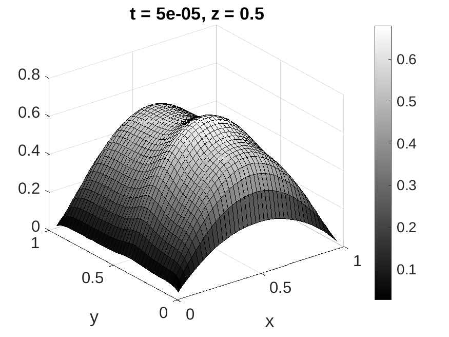
Figure 4: Left: initial value function $u(x,y,z,0)$ of the Bratu test on a uniform $40\times 40\times 40$ grid for $z=0.5$. Right: numerical solution $u(x,y,z,t)$ on the same grid for $z=0.5$ and $t=5\cdot 10^{-5}$.

The regular second order finite-difference discretization of the spatial derivatives in (30) on a uniform grid yields an IVP

$$y^{\prime}(t)=-Ay(t)+\hat{f}(y(t))+g(t),\quad y(0)=v,$$ (31)

where the entries of the vector functions $y(t)$ and $g(t)$ contain the values of the numerical solution and function $\tilde{g}(x,y,z,t)$ at the grid nodes, respectively, and

$$Ay(t)\approx-(10^{4}u_{xx}+10^{2}u_{yy}+u_{zz}).$$

Furthermore, the components $[\hat{f}(y)]_{i}$ of the vector function $\hat{f}(y)$ are defined as

$$\left[\hat{f}(y)\right]_{i}=Ce^{y_{i}},\quad i=1,\dots,n.$$

To apply nonlinear waveform relaxation (8) for solving (31), one could have chosen to set $A_{k}:=A$ and $f_{k}(y):=\hat{f}(y)$. However, to have a smaller Lipschitz constant $L$ in $f_{k}(y)$, we supplement $A$ with a linear part of $\hat{f}$, setting

$$y_{k+1}^{\prime}(t)=-(\,\underbrace{A-J(\bar{y}_{k})}_{\displaystyle A_{k}}\,)y_{k+1}(t)+\underbrace{\left[\hat{f}(y_{k}(t))-J(\bar{y}_{k})y_{k}(t)\right]}_{\displaystyle f_{k}(y_{k}(t))}+g(t),$$ (32)

$$k=0,1,2,\dots,$$

where $J(\bar{y}_{k})$ is the Jacobian matrix of $\hat{f}(y)$ evaluated at $\bar{y}_{k}=y_{k}(T)$ and an approximation

$$\hat{f}(y_{k+1}(t))\approx\hat{f}(y_{k}(t))+J(\bar{y}_{k})(y_{k+1}(t)-y_{k}(t))$$

is used. The nonlinear residual (16) takes in this case the form, for $k=0,1,\dots$,

$$r_{k+1}(t) =f_{k}(y_{k+1}(t))-f_{k}(y_{k}(t))$$

$$=\left[\hat{f}(y_{k+1}(t))-J(\bar{y}_{k})y_{k+1}(t)\right]-\left[\hat{f}(y_{k}(t))-J(\bar{y}_{k})y_{k}(t)\right]$$

$$=\hat{f}(y_{k+1}(t))-\hat{f}(y_{k}(t))-J(\bar{y}_{k})(y_{k+1}(t)-y_{k}(t)).$$

The iterations are stopped provided that $\|r_{k}(T)\|\leqslant\texttt{tol}$ for the tolerance tol set in this test to $10^{-2}$.

The low rank representation (26) at each iteration $k$ is computed at $s=100$ sample points $t_{j}$, $j=1,\dots,s$ for either $m=4$ or $m=5$ low rank terms. The residual tolerance in the EBK solver applied to solve (8) is defined as $\texttt{tol}_{\mathtt{EBK}}=\texttt{tol}$ and Krylov subspace dimension is set to $10$. Hence, for the block size $m=5$, the EBK solver has to store $5\cdot(10+1)=55$ vectors. Since the problem is stiff, just as in the previous test, the EBK solver is employed in the SAI mode, with a sparse LU factorization of $I+\gamma A$ computed and applied throughout each nonlinear iteration. The relative error values we report below are computed according to (29).

We compare our nonlinear EBK solver to the two-stage Rosenbrock method ROS2, see [10] or [1, Chapter IV.5]. For IVP (1), it can be written as

$$y^{\ell+1} =y^{\ell}+\frac{3}{2}\tau k_{1}+\frac{1}{2}\tau k_{2},$$ (33)

$$(I-\gamma\tau\widehat{A})k_{1} =F(t_{\ell},y^{\ell}),$$

$$(I-\gamma\tau\widehat{A})k_{2} =F(t_{\ell+1},y^{\ell}+\tau k_{1})-2k_{1}.$$

Here $y^{\ell}\approx y(\ell\tau)$ is numerical solution at time step $\ell=0,1,2,\dots$ ($y^{0}=v$) obtained with a time step size $\tau>0$. This scheme is second order consistent for any matrix $\widehat{A}\in\mathbb{R}^{n\times n}$. Here we take $\widehat{A}$ to be the Jacobian matrix of $F$ computed at $t_{\ell}=\ell\tau$ and $y_{\ell}$. At each time step a sparse LU factorization of $I-\gamma\tau\widehat{A}$ can be computed and used to solve the two linear systems in $k_{1,2}$. The numerical tests presented here are carried in Matlab and, as it turns out, for the grid sizes used, it is much faster to compute the action of the matrix $(I-\gamma\tau\widehat{A})^{-1}$ by the Matlab backslash operator \ than to compute a sparse LU factorization first and to apply it twice. This is apparently because Matlab creates an overhead to call sparse LU factorization routines (of the UMFPACK software [47, 48]) and then to store the computed LU factors as Matlab variables. Note that both the backslash operator as well as the LU factorization for large sparse matrices in Matlab are based on UMFPACK.

Comparison results of our nonlinear EBK solver and ROS2 method are presented in Table 3. The results clearly show that, for this test problem, the nonlinear EBK solver is much more efficient than the ROS2 method both in terms of required LU factorizations (and their actions) and the CPU time. We also see that the number of nonlinear waveform relaxation iterations does change with grid size and with final time $T$. While the convergence independence on the grid size is expected (as the grid size does not affect the nonlinear part $Ce^{u}$ in the ODE), the weak convergence dependence on $T$ is probably a property of the specific test problem. From plots in Figure 5 we see that convergence behavior does change with $T$.

Table 3: The 3D Bratu test problem. Attained error and computational work for our nonlinear EBK method and the ROS2 solver. For the EBK method the work is reported as the nonlinear iteration number, number of LU factorizations, their applications and matvecs. For the ROS2 solver the work is shown as the number of LU factorizations and their applications (two per time step).

method,	iter./	LUs (LUs applic.),	relative	CPU
tolerance / $\tau$	steps	matvecs/fevals	error	time, s
grid $40\times 40\times 40$, $T=5\cdot 10^{-5}$, $\|A(y(T))\|_{1}\approx\texttt{6.79e+07}$
nonlin.EBK($m=4$), 1e-02	4	4 (131), 4	6.21e-05	41
nonlin.EBK($m=5$), 1e-02	4	4 (161), 4	1.22e-05	42
ROS2, $\tau=T/320$	320	320 (640), 640	2.36e-04	225
ROS2, $\tau=T/640$	640	640 (1280), 1280	5.73e-07	442
grid $40\times 40\times 40$, $T=1\cdot 10^{-4}$, $\|A(y(T))\|_{1}\approx\texttt{6.79e+07}$
nonlin.EBK($m=4$), 1e-02	4	4 (131), 4	2.19e-05	40
nonlin.EBK($m=5$), 1e-02	4	4 (161), 4	1.52e-05	43
ROS2, $\tau=T/320$	320	320 (640), 640	1.51e-05	201
ROS2, $\tau=T/640$	320	640 (1280), 1280	7.51e-06	401
grid $60\times 60\times 60$, $T=5\cdot 10^{-5}$, $\|A(y(T))\|_{1}\approx\texttt{1.50e+08}$
nonlin.EBK($m=4$), 1e-02	4	4 (131), 4	6.16e-05	288
nonlin.EBK($m=5$), 1e-02	4	4 (161), 4	1.23e-05	308
ROS2, $\tau=T/320$	320	320 (640), 640	2.35e-04	2177
ROS2, $\tau=T/640$	640	640 (1280), 1280	1.66e-05	4790
grid $60\times 60\times 60$, $T=1\cdot 10^{-4}$, $\|A(y(T))\|_{1}\approx\texttt{1.50e+08}$
nonlin.EBK($m=4$), 1e-02	4	4 (131), 4	2.16e-05	288
nonlin.EBK($m=5$), 1e-02	4	4 (161), 4	1.53e-05	310
ROS2, $\tau=T/320$	320	320 (640), 640	2.11e-05	2013
ROS2, $\tau=T/640$	640	640 (1280), 1280	1.66e-05	4368

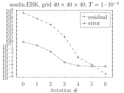
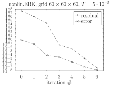
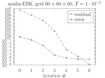
Figure 5: The Bratu 3D test. Residual and error norm versus iteration number in the nonlinear EBK solver for the grid size $40\times 40\times 40$ (top plots) and $60\times 60\times 60$ (bottom plots), $T=5\cdot 10^{-5}$ (left plots) and $T=1\cdot 10^{-4}$ (right plots). The plots are made with an increased block size $m=12$.

Results presented in Table 3 for the nonlinear EBK solver are obtained with the block size $m=4$ and $m=5$. The value $m=4$ is marginally acceptable for the accuracy point of view but does yield an acceptable error values. Therefore, the plots in Figure 5, made to get an insight in the error convergence, are produced with a larger block size $m=12$.

Finally, we briefly comment on convergence of the ROS2 method. Since its convergence order can not be seen from error values shown in Table 3, we give an error convergence plot in Figure 6, where relative error values, computed as given in (29), are plotted versus the corresponding time step sizes. The second order convergence is clearly seen.

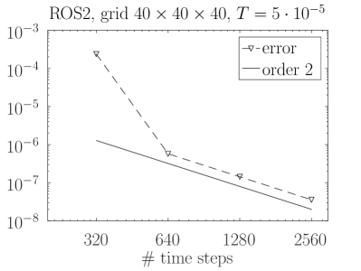
Figure 6: The Bratu 3D test. Relative error of the ROS2 method, computed as given in (29), versus the time step size.

4 Conclusions

In this paper nonlinear waveform relaxation iterations and their block Krylov subspace implementation (the nonlinear EBK method) are examined theoretically and practically. Theoretically we have shown that convergence of the considered nonlinear waveform relaxation iteration is determined by the Lipschitz constant $L$ of the nonlinear term $f_{k}$ in (3), the logarithmic norm bound $\omega$ of the linear term matrix $A_{k}$ and the time interval length $T$, see relation (10). We have also established a superlinear convergence of our nonlinear iteration, which is known to hold in the linear case, see Proposition 2. Furthermore, we have linked the residual convergence in the nonlinear iteration to the error convergence, see relation (20). Finally, it is shown that inexact solution of the linear initial-value problem arising at each waveforem relaxation iteration leads to a process whose convergence is equivalent to convergence of the exact waveforem relaxation iteration with an increased Lipschitz constant $L+l$, with $l$ being the inexactness tolerance.

Practical performance of nonlinear waveform relaxation heavily depends on the ability to solve the arising linear initial-value problem at each relaxation iteration quickly and to handle the iterative across-time solutions efficiently. As we show here, both these goals can be successfully reached by employing the exponential block Krylov subspace method EBK [37]. In the presented experiments the EBK method is used in the shift-and-invert (SAI) mode, i.e., it has been assumed that the SAI linear systems (similar to those arising in implicit time stepping) can be solved efficiently.

Comparisons with implicit time integration methods demonstated superiority and potential of our EBK-SAI based nonlinear waveform relaxation iterations. The presented nonlinear residual stopping criterion has been proven to be a reliable way to control convergence and to estimate accuracy. Moreover, as numerical tests demonstrate, the grid independent convergence of linear SAI Krylov subspace exponential time integrators (see [49, 44, 50]) is inherited by the nonlinear waveform relaxation iterations.

Nevertheless, some tuning (such as a proper choice of the block size $m$ and the time interval lengtgh $T$) is required to apply the proposed approach successfully. These issues can be addressed in more details in a future.

Recently, an alternative approach based on exponential Krylov subspace integrators has been presented in [51] for nonlinear heat equations. In this problem a rapid change in the solution seems to exclude using waveform relaxation with block Krylov subspaces as presented here. A further research should be done to get an insight on when to switch between the block Krylov subpace approach discussed here and the approach of [51]. Finally, it seems to be useful to gain more insight how these two approaches compare to other exponential time integrators for nonlinear initial-value problems [3, 52, 53].

References

- \bibcommenthead
- [1] W. Hundsdorfer, J.G. Verwer, Numerical Solution of Time-Dependent Advection-Diffusion-Reaction Equations (Springer Verlag, 2003)
- [2] H.C. Elman, D.J. Silvester, A.J. Wathen, Finite Elements and Fast Iterative Solvers with Applications in Incompressible Fluid Dynamics (Oxford University Press, Oxford, 2005)
- [3] M. Hochbruck, A. Ostermann, Exponential integrators. Acta Numer. 19, 209–286 (2010). 10.1017/S0962492910000048
- [4] P.N. Brown, Y. Saad, Convergence theory of nonlinear Newton–Krylov algorithms. SIAM J. Optimization 4(2), 297–330 (1994)
- [5] R. Choquet, J. Erhel, Newton–GMRES algorithm applied to compressible flows. Int. J. Numer. Meth. Fluids 23, 177–190 (1996)
- [6] D. Tromeur-Dervout, Y. Vassilevski, Choice of initial guess in iterative solution of series of systems arising in fluid flow simulations. Journal of Computational Physics 219(1), 210–227 (2006). https://doi.org/10.1016/j.jcp.2006.03.014. URL https://www.sciencedirect.com/science/article/pii/S0021999106001483
- [7] N.N. Yanenko, The method of fractional steps. The solution of problems of mathematical physics in several variables (Springer-Verlag, New York, 1971), pp. viii+160
- [8] E.G. D’yakonov, Difference systems of second order accuracy with a divided operator for parabolic equations without mixed derivatives. USSR Comput. Math. Math. Phys. 4(5), 206–216 (1964)
- [9] P. Csomós, I. Faragó, A. Havasi, Weighted sequential splittings and their analysis. Comput. Math. Appl. pp. 1017–1031 (2005)
- [10] J.G. Verwer, E.J. Spee, J.G. Blom, W. Hundsdorfer, A second order Rosenbrock method applied to photochemical dispersion problems. SIAM J. Sci. Comput. 20, 456–480 (1999)
- [11] P.J. van der Houwen, B.P. Sommeijer, On the internal stability of explicit -stage Runge–Kutta methods for large values of . Z. Angew. Math. Mech. 60, 479–485 (1980)
- [12] V.O. Lokutsievskii, O.V. Lokutsievskii, On numerical solution of boundary value problems for equations of parabolic type. Soviet Math. Dokl. 34(3), 512–516 (1987)
- [13] B.P. Sommeijer, L.F. Shampine, J.G. Verwer, RKC: An explicit solver for parabolic PDEs. J. Comput. Appl. Math. 88, 315–326 (1998)
- [14] H. Tal-Ezer, Spectral methods in time for parabolic problems. SIAM J. Numer. Anal. 26(1), 1–11 (1989)
- [15] V.I. Lebedev, Explicit difference schemes for solving stiff systems of ODEs and PDEs with complex spectrum. Russian J. Numer. Anal. Math. Modelling 13(2), 107–116 (1998). 10.1515/rnam.1998.13.2.107
- [16] J.G. Verwer, B.P. Sommeijer, W. Hundsdorfer, RKC time-stepping for advection–diffusion–reaction problems. Journal of Computational Physics 201(1), 61–79 (2004). https://doi.org/10.1016/j.jcp.2004.05.002. URL https://www.sciencedirect.com/science/article/pii/S0021999104001925
- [17] M.A. Botchev, G.L.G. Sleijpen, H.A. van der Vorst, Stability control for approximate implicit time stepping schemes with minimum residual iterations. Appl. Numer. Math. 31(3), 239–253 (1999). https://doi.org/10.1016/S0168-9274(98)00138-X
- [18] M.A. Botchev, H.A. van der Vorst, A parallel nearly implicit scheme. Journal of Computational and Applied Mathematics 137, 229–243 (2001). https://doi.org/10.1016/S0377-0427(01)00358-2
- [19] V.T. Zhukov, Explicit methods of numerical integration for parabolic equations. Mathematical Models and Computer Simulations 3(3), 311–332 (2011). https://doi.org/10.1134/S2070048211030136
- [20] E. Lelarasmee, A.E. Ruehli, A.L. Sangiovanni-Vincentelli, The waveform relaxation method for time-domain analysis of large scale integrated circuits. IEEE Transactions on Computer-Aided Design of Integrated Circuits and Systems 1(3), 131–145 (1982). 10.1109/TCAD.1982.1270004
- [21] A.R. Newton, A.L. Sangiovanni-Vincentelli, Relaxation-based electrical simulation. IEEE Transactions on Electron Devices 30(9), 1184–1207 (1983). 10.1109/T-ED.1983.21275
- [22] S. Vandewalle, Parallel Multigrid Waveform Relaxation for Parabolic Problems (Teubner, Stuttgart, 1993)
- [23] U. Miekkala, O. Nevanlinna, Iterative solution of systems of linear differential equations. Acta Numerica 5, 259–307 (1996). https://doi.org/10.1017/S096249290000266X
- [24] J. White, F. Odeh, A.L. Sangiovanni-Vincentelli, A. Ruehli, Waveform relaxation: Theory and practice. Tech. Rep. UCB/ERL M85/65, EECS Department, University of California, Berkeley (1985). www.eecs.berkeley.edu/Pubs/TechRpts/1985/543.html
- [25] U. Miekkala, O. Nevanlinna, Convergence of dynamic iteration methods for initial value problems. SIAM Journal on Scientific and Statistical Computing 8(4), 459–482 (1987). https://doi.org/10.1137/0908046
- [26] C. Lubich, A. Ostermann, Multi-grid dynamic iteration for parabolic equations. BIT Numerical Mathematics 27, 216–234 (1987). URL http://doi.org/10.1007/BF01934186. 10.1007/BF01934186
- [27] J. Janssen, S. Vandewalle, Multigrid waveform relaxation of spatial finite element meshes: The continuous-time case. SIAM J. Numer. Anal. 33(2), 456–474 (1996). 10.1137/0733024
- [28] M.J. Gander, S. Güttel, PARAEXP: A parallel integrator for linear initial-value problems. SIAM Journal on Scientific Computing 35(2), C123–C142 (2013)
- [29] G.L. Kooij, M.A. Botchev, B.J. Geurts, A block Krylov subspace implementation of the time-parallel Paraexp method and its extension for nonlinear partial differential equations. Journal of Computational and Applied Mathematics 316(Supplement C), 229–246 (2017). https://doi.org/10.1016/j.cam.2016.09.036
- [30] G. Kooij, M.A. Botchev, B.J. Geurts, An exponential time integrator for the incompressible Navier–Stokes equation. SIAM J. Sci. Comput. 40(3), B684–B705 (2018). https://doi.org/10.1137/17M1121950
- [31] T.J. Park, J.C. Light, Unitary quantum time evolution by iterative Lanczos reduction. J. Chem. Phys. 85, 5870–5876 (1986)
- [32] H.A. van der Vorst, An iterative solution method for solving , using Krylov subspace information obtained for the symmetric positive definite matrix . J. Comput. Appl. Math. 18, 249–263 (1987)
- [33] V.L. Druskin, L.A. Knizhnerman, Two polynomial methods of calculating functions of symmetric matrices. U.S.S.R. Comput. Maths. Math. Phys. 29(6), 112–121 (1989)
- [34] E. Gallopoulos, Y. Saad, Efficient solution of parabolic equations by Krylov approximation methods. SIAM J. Sci. Statist. Comput. 13(5), 1236–1264 (1992). http://doi.org/10.1137/0913071
- [35] V.L. Druskin, L.A. Knizhnerman, Krylov subspace approximations of eigenpairs and matrix functions in exact and computer arithmetic. Numer. Lin. Alg. Appl. 2, 205–217 (1995)
- [36] M. Hochbruck, C. Lubich, On Krylov subspace approximations to the matrix exponential operator. SIAM J. Numer. Anal. 34(5), 1911–1925 (1997)
- [37] M.A. Botchev, A block Krylov subspace time-exact solution method for linear ordinary differential equation systems. Numer. Linear Algebra Appl. 20(4), 557–574 (2013). http://doi.org/10.1002/nla.1865
- [38] O. Nevanlinna, F. Odeh, Remarks on the convergence of waveform relaxation method. Numerical functional analysis and optimization 9(3-4), 435–445 (1987). https://doi.org/10.1080/01630568708816241
- [39] K. Dekker, J.G. Verwer, Stability of Runge–Kutta methods for stiff non-linear differential equations (North-Holland Elsevier Science Publishers, 1984)
- [40] M.A. Botchev, V. Grimm, M. Hochbruck, Residual, restarting and Richardson iteration for the matrix exponential. SIAM J. Sci. Comput. 35(3), A1376–A1397 (2013). http://doi.org/10.1137/110820191
- [41] M.A. Botchev, I.V. Oseledets, E.E. Tyrtyshnikov, Iterative across-time solution of linear differential equations: Krylov subspace versus waveform relaxation. Computers & Mathematics with Applications 67(12), 2088–2098 (2014). http://doi.org/10.1016/j.camwa.2014.03.002
- [42] E. Hairer, G. Wanner, Solving Ordinary Differential Equations II. Stiff and Differential–Algebraic Problems, 2nd edn. Springer Series in Computational Mathematics 14 (Springer–Verlag, 1996)
- [43] L.A. Krukier, Implicit difference schemes and an iterative method for solving them for a certain class of systems of quasi-linear equations. Sov. Math. 23(7), 43–55 (1979). Translation from Izv. Vyssh. Uchebn. Zaved., Mat. 1979, No. 7(206), 41–52 (1979)
- [44] J. van den Eshof, M. Hochbruck, Preconditioning Lanczos approximations to the matrix exponential. SIAM J. Sci. Comput. 27(4), 1438–1457 (2006)
- [45] L.F. Shampine, M.W. Reichelt, The MATLAB ODE suite. SIAM J. Sci. Comput. 18(1), 1–22 (1997). Available at www.mathworks.com
- [46] J. Jon, S. Klaus, The Liouville–Bratu–Gelfand problem for radial operators. Journal of Differential Equations 184, 283–298 (2002). https://doi.org/10.1006/jdeq.2001.4151
- [47] T.A. Davis, A column pre-ordering strategy for the unsymmetric-pattern multifrontal method. ACM Trans. Math. Software 30(2), 167–195 (2004). 10.1145/992200.992205
- [48] T.A. Davis, Algorithm 832: UMFPACK V4.3—an unsymmetric-pattern multifrontal method. ACM Trans. Math. Software 30(2), 196–199 (2004). 10.1145/992200.992206
- [49] I. Moret, P. Novati, RD rational approximations of the matrix exponential. BIT 44, 595–615 (2004)
- [50] V. Grimm, Resolvent Krylov subspace approximation to operator functions. BIT 52(3), 639–659 (2012). 10.1007/s10543-011-0367-8
- [51] M.A. Botchev, V.T. Zhukov, Exponential Euler and backward Euler methods for nonlinear heat conduction problems. Lobachevskii Journal of Mathematics 44(1), 10–19 (2023). https://doi.org/10.1134/S1995080223010067
- [52] D. Hipp, M. Hochbruck, A. Ostermann, An exponential integrator for non-autonomous parabolic problems. ETNA 41, 497–511 (2014). http://etna.mcs.kent.edu/volumes/2011-2020/vol41/
- [53] E. Hansen, A. Ostermann, High-order splitting schemes for semilinear evolution equations. BIT Numerical Mathematics 56(4), 1303–1316 (2016)