AE-RED: A Hyperspectral Unmixing Framework Powered by Deep Autoencoder and Regularization by Denoising

Abstract

Spectral unmixing has been extensively studied with a variety of methods and used in many applications. Recently, data-driven techniques with deep learning methods have obtained great attention to spectral unmixing for its superior learning ability to automatically learn the structure information. In particular, autoencoder based architectures are elaborately designed to solve blind unmixing and model complex nonlinear mixtures. Nevertheless, these methods perform unmixing task as black-boxes and lack of interpretability. On the other hand, conventional unmixing methods carefully design the regularizer to add explicit information, in which algorithms such as plug-and-play (PnP) strategies utilize off-the-shelf denoisers to plug powerful priors. In this paper, we propose a generic unmixing framework to integrate the autoencoder network with regularization by denoising (RED), named AE-RED. More specially, we decompose the unmixing optimized problem into two subproblems. The first one is solved using deep autoencoders to implicitly regularize the estimates and model the mixture mechanism. The second one leverages the denoiser to bring in the explicit information. In this way, both the characteristics of the deep autoencoder based unmixing methods and priors provided by denoisers are merged into our well-designed framework to enhance the unmixing performance. Experiment results on both synthetic and real data sets show the superiority of our proposed framework compared with state-of-the-art unmixing approaches.

TABLE I: Notations.

$x$, $X$	scalar
$\mathbf{x}$	column vector
$\mathbf{X}$	matrix
$B$	number of spectral bands
$N$	number of pixels
$R$	number of endmembers
$\mathbf{y}_{i}\in\mathbb{R}^{B}$	spectrum of the $i$th observed pixel
$\mathbf{Y}\in\mathbb{R}^{B\times N}$	an observed hyperspectral image
$\mathbf{a}_{i}\in\mathbb{R}^{R}$	abundance vector of the $i$th pixel
$\mathbf{A}\in\mathbb{R}^{R\times N}$	abundance matrix of all pixels
$\mathbf{S}\in\mathbb{R}^{B\times R}$	endmember matrix with $R$ spectral signatures
$\bm{1}$	all one vector or matrix
$\bm{0}$	all zero vector or matrix
$\cdot\geq\cdot$	elementwise inequality between vectors or matrices

I Introduction

Hyperspectral imaging has been a widely explored imaging technique during recent years and is still receiving a growing attention in various applicative fields [1, 2]. Benefiting from the rich spectral information, hyperspectral images enable the analysis of fine materials in the observed scenes to tackle various challenging tasks such as target detection and classification [3, 4]. However, due to the limitations of the imaging acquisition devices, there is an unsurmountable trade-off between the collected spectral and spatial information, which limits the spatial resolution of the hyperspectral sensors. As a consequence, a pixel observed by a hyperspectral sensor generally corresponds to a relatively large area and may encompass several materials, in particular when observing complex scenes. More precisely, the spectrum collected at a given spatial position of the scene is assumed to be a mixture of several elementary spectral signatures associated with the materials present in the observed pixel. This has led to research focused on hyperspectral unmixing (HU), which aims at decomposing the $i$th observed pixel spectrum $\mathbf{y}_{i}\in\mathbb{R}^{B}$ into a set of $R$ spectral signatures of so-called endmembers collected in the matrix $\mathbf{S}=\left[\mathbf{s}_{1},\ldots,\mathbf{s}_{R}\right]\in\mathbb{R}^{B\times R}$ and their associated fractions or abundances $\mathbf{a}_{i}\in\mathbb{R}^{R}$ [5, 6, 7]. For the sake of physical interpretability, the abundances are subject to two constraints, namely abundance sum-to-one constraint (ASC), $\bm{1}_{R}^{\top}\mathbf{a}_{i}=1$, and abundance nonnegativity constraint (ANC), $\mathbf{a}_{i}\geq\bm{0}$. The endmembers are constrained to be nonnegative (ENC), $\mathbf{S}\geq\bm{0}$.

Many methods have been proposed in the literature to address the HU problem [8, 9, 10, 11, 12]. Considering a set of $N$ observed pixels $\mathbf{Y}=\left[\mathbf{y}_{1},\ldots,\mathbf{y}_{N}\right]\in\mathbb{R}^{B\times N}$ sharing the same endmembers, HU can be formulated as an optimization problem, which aims at estimating the endmembers $\mathbf{S}$ and the abundances $\mathbf{A}$ jointly, i.e.,

$$\begin{split}&\mathop{\rm min}_{\mathbf{S},\mathbf{A}}\quad\sum_{i=1}^{N}\mathcal{D}\left[\mathbf{y}_{i}\big{|}\big{|}{\mathcal{M}}\big{(}\mathbf{S},\mathbf{a}_{i})\big{)}\right]+\mathcal{R}\big{(}\mathbf{S},\mathbf{A}\big{)}\\ &\qquad\;\;{\rm s.t.}\quad\bm{1}_{R}^{\top}\mathbf{A}=\bm{1}_{N}^{\top},~{}\mathbf{A}\geq\bm{0},~{}\text{and}~{}\mathbf{S}\geq\bm{0}\end{split}$$ (1)

where

• $\mathcal{D}(\cdot,\cdot)$ stands for a discrepancy measure (e.g., divergence),

• $\mathcal{M}(\cdot,\cdot)$ describes the inherent nonlinear mixture model which relates the endmembers and the abundances to the measurements,

• $\mathcal{R}(\cdot,\cdot)$ acts as a regularization term that encodes prior information regarding the endmembers $\mathbf{S}$ and the abundances $\mathbf{A}$.

The regularization $\mathcal{R}(\cdot,\cdot)$ is often designed to be separable with respect to the abundances and endmembers,

$$\mathcal{R}(\mathbf{S},\mathbf{A})=\mathcal{R}_{\rm e}(\mathbf{S})+\mathcal{R}_{\rm a}(\mathbf{A}),$$ (2)

where the endmember and abundance prior information is encoded in $\mathcal{R}_{\rm e}$ and $\mathcal{R}_{\rm a}$, respectively. For instance, geometry-based penalizations, such as minimum volume [13], are often chosen as endmember regularizers. Sparsity-based  [14], low-rankness  [15] or spatial regularizers, such as total variation (TV) [16], are usually utilized to promote expected properties of the abundances. This work specifically focuses on the design of an abundance regularization.

As for the mixing process, typical methods rely on an explicit mathematical expression for $\mathcal{M}(\cdot,\cdot)$ to describe the mixture mechanism. For example, the linear mixing model (LMM) is by far the most used in the literature since it provides a generally admissible first-order approximation of the physical processes underlying the observations. LMM assumes that the measured spectrum is a linear combination of endmembers weighted by the abundances, which assumes that the incident light comes in and only reflects once on the ground before reaching the hyperspectral sensor. Besides, bilinear models consider second-order reflections, for instance in the case of multiple vegetation layers [17, 1]. These explicit models are usually designed by describing the path of the light, along with its scattering and the interaction mechanisms among the materials. They are thus generally referred to as physics-based models. However, in some acquisition scenarios, they may fail to accurately account for real complex scenes. Data-driven methods have been thus proposed to implicitly learn the mixing mechanism from the observed data. Nevertheless, if not carefully designed a data-driven method may overlook the physical mixing process and require abundant training data [18].

I-A Motivation

Numerous methods cope with the HU problem by carefully designing the data-fitting term and the regularizer [19, 20]. To reduce the computational complexity, most HU methods are based on the LMM. It may be not sufficient to account for spectral variability and endmember nonlinearity. On the other hand, designing a relevant regularizer is not always trivial and is generally driven by an empirical yet limited knowledge. For these reasons, research works have been devoted to the design of deep learning based HU approaches. Among them, autoencoders (AEs) become increasingly popular for unsupervised HU. The encoder is trained to compress the input into a lower dimensional latent representation, usually the abundances. The decoder is generally designed to mimic the mixing process parametrized by the endmember signatures and to produce the hyperspectral image from the abundances defined in the latent space. AE-based HU methods exhibit several advantages: i) they can embed a physical-based mixing model into the structure of the decoder, ii) they implicitly incorporates data-driven image priors and iii) the unmixing procedure can benefit from powerful optimizers, such as Adam [21] and SGD [22]. However, these deep architectures behave as black boxes and the results lack of interpretation. Motivated by these findings, this paper attempts to answer the following question: is it possible to design an unsupervised HU framework which combines the advantages of AE-based unmixing network while leveraging on explicit priors?

I-B Contributions

This paper derives a novel HU framework which answers to this question affirmatively. More precisely, it introduces an AE-based unmixing strategy while incorporating an explicit regularization of the form of a RED. To solve the resulting optimization problem, an alternating direction method of multiplier (ADMM) is implemented with the great advantages of decomposing the initial problem into several simpler subproblems. One of these subproblems can be interpretated as a standard training task associated with an AE. Another is a standard denoising problem. The main advantages of the proposed frameworks are threefold:

• This framework combines the deep AE with RED priors for unsupervised HU. By incorporating the benefits of AE with the regularization of denoising, the framework provides accurate unmixing results.

• The optimization procedure splits the unmixing task into two main subtasks. The first subtask involves training an AE to learn the mixing process and estimate a latent representation of the image as abundance maps. In the second subtask, a denoising step is applied to improve the estimation of the latent representation.

• The proposed framework is highly versatile and can accommodate various architectures for the encoder, and the decoder can be tailored to mimic any physics-based mixing model, such as the LMM, nonlinear mixing models, and mixing models with spectral variability.

This paper is organized as follows. Section II provides a concise overview of related HU algorithms, with a particular focus on the design of regularizations and AE-based unmixing methods. Section III describes some technical ingredients necessary to build the proposed framework. In Section IV, the proposed generic framework is derived, and details about particular instances of this framework are given. Section V reports the results obtained from extensive experiments conducted on synthetic and real datasets to demonstrate the superiority of the proposed framework. Finally, Section VI concludes the paper.

II Related works

This section provides brief overviews on two aspects related to this work, namely regularization design in HU and AE-based unmixing.

II-A Regularization design

Efficient algorithms for HU often require effective regularizations that incorporate prior knowledge about the images and constrain the solution space. Traditional methods exploit the spatial consistency of the image, and sparsity-based regularizers have also been extensively used on the abundances since the number of endmembers is typically much smaller than the size of the spectral library.

In [16], a TV regularizer is applied to the abundance to promote similarity between adjacent pixels, and an $\ell_{1}$-norm is used for sparse unmixing. Since the $\ell_{1}$-norm is inconsistent with the abundance sum-to-one constraint, $\ell_{p}$-norms with $0<p<1$ have been studied to obtain sparse estimates [23]. In [24], a non-local sparse unmixing method is proposed to exploit similar patterns and structures in the abundance image. A weighted average is applied to all pixels to exploit non-local spatial information. A weighted average is applied to all pixels to exploit non-local spatial information. Spatial group sparsity regularizers have also been proposed to incorporate spatial priors and sparse structures. The authors of [25] introduce a spatial group sparsity regularizer generated using image segmentation methods such as SLIC. In [26], a cofactorization model is used to jointly exploit spectral and spatial information, while the work of [27] introduces an adaptive graph to automatically determine the best neighbor points of pixels and assign corresponding weights. However, these methods require handcrafted regularizers, which can be time-consuming when non-standard regularizers are applied to large images.

More recently, the idea of PnP has been introduced to exploit the intrinsic properties of hyperspectral images. These methods use generic denoisers that act as explicit regularizers. In [28], an HU method based on an ADMM algorithm is introduced that can handle explicit regularizations. By selecting different pattern switch matrices, the denoising operator can be used to penalize the reconstructed hyperspectral image or estimated abundances. The work of [29] proposes a nonlinear unmixing method with prior information provided by denoisers. However, the denoisers used in these methods are traditional denoising methods or deep denoisers trained on grayscale or RGB images, which may not be optimal for hyperspectral images.

II-B Deep AE-based unmixing methods

Elegant neural network structures have been proposed to formulate the HU task as a simple training process. Early works used fully connected layers to design the model, such as [12] and [30]. However, these networks process the pixels independently and ignore the spatial correlation intrinsic to the image. To overcome this limitation, some AE-based methods include spatial regularizations, such as total variation (TV), in the loss function [31]. Recently, convolutional neural networks (CNNs) have been used to perform HU and have shown promising performance. CNNs convolve the input data with filter kernels to capture spatial information [10, 32]. Recurrent neural networks (RNNs), which have memory cells, implement a sequential process with hidden states that depend on the previous states [31]. Hyperspectral images are often corrupted by noise or outliers, which can dramatically decrease the unmixing performance. To address this issue, denoising-oriented architectures have been proposed [30]. Some works have also proposed variants of encoders. In [33], a dual-branch AE network is designed to leverage multiscale spatial contextual information.

Most AE-based HU methods use a fully connected linear layer in the decoder part to mimic the linear mixing process. However, considering the physical interactions between multiple materials and the superior ability of deep networks to model nonlinear relationships, some works [34, 32, 31, 35] have focused on the design of structured decoders to ensure the interpretability of the nonlinear model inherent in the mixing process. The work of [34] introduces a nonlinear decoder. Recycling an LMM-based AE architecture, the decoder contains two parts: one linear and the other nonlinear. The linear part is considered a rough approximation of the mixture and is then fed into two fully connected layers with a nonlinear activation function to learn the nonlinear mechanism. However, this post-nonlinear model-based decoder may not be sufficient to represent complex nonlinear cases. Some works [32, 31, 35] reexamine the nonlinear fluctuation part of the decoder. For example, the method in [35] designs a special layer to capture the second-order interaction, similar to the Fan or bilinear models. Moreover, spectral variability can also be addressed by using deep generative decoders [36, 37].

Recently, deep unfolding techniques have been used to unroll a model and its related iterative algorithm into deep networks. This approach can include physical interpretability into the design of network layers, and such model-inspired networks are also used in the design of unmixing methods. In [38], an iterative shrinkage-thresholding algorithm (ISTA)-inspired network layer is applied to build an AE-based unmixing architecture. The work of [39] unrolls a sparse non-negative matrix factorization (NMF)-based algorithm with an $\ell_{p}$-norm regularizer to integrate prior knowledge into the unmixing network. An ADMM solver with a sparse regularizer is also unrolled to build an AE-like unmixing architecture. However, these methods do not utilize spatial consistency information in the design of the network, which may limit their unmixing performance.

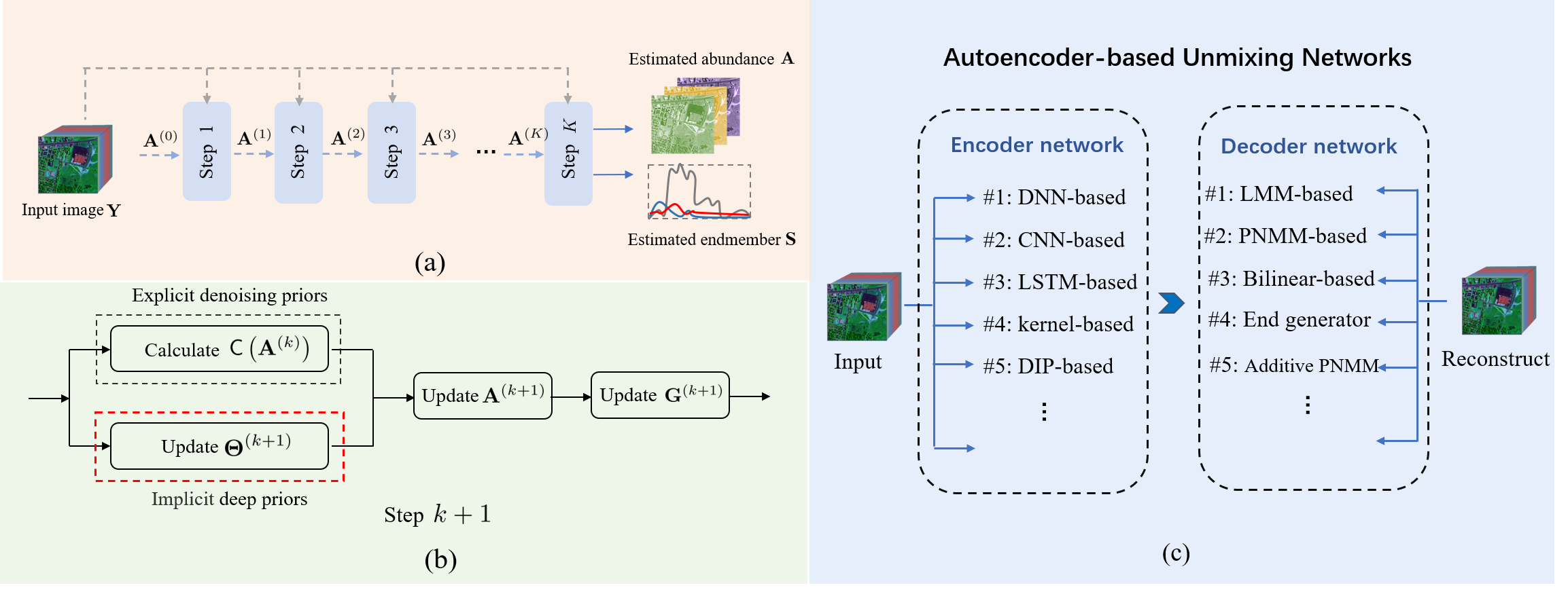
Figure 1: Framework of the proposed AE-RED. (a) The scheme of the proposed framework. (b) Flowchart of the $(k+1)$th ADMM step: the denoising operator is applied in parallel to the update of $\bm{\Theta}$ to speed up calculations. (c) An overview and some instances of AE-based unmixing networks, where the encoder embeds deep priors for abundance estimation, and the decoder can model the mixture mechanism and extract the endmembers. The choice of the encoder and decoder is let to the end-user.

III Background

III-A Autoencoder-based unmixing

As highlighted in the previous section, AEs have demonstrated to be a powerful tool to conduct unsupervised unmixing. An AE typically consists of an encoder and a decoder. The encoder, represented by $\mathsf{E}_{\bm{\Theta}_{\sf E}}(\cdot)$, aims at learning a nonlinear mapping from input data, denoted as $\mathbf{w}_{i}$, to their corresponding latent representations, denoted as $\mathbf{v}_{i}$. This can be expressed as follows:

$$\mathbf{v}_{i}=\mathsf{E}_{\bm{\Theta}_{\sf E}}(\mathbf{w}_{i}),$$ (3)

where $\bm{\Theta}_{\sf E}$ gather all parameters of the encoder. The input $\mathbf{W}=\left[\mathbf{w}_{1},\ldots,\mathbf{w}_{N}\right]$ depends on the architecture chosen for the encoder network. For instance, when dealing with the specific task of HU, the input can be chosen as the image pixels $\mathbf{Y}=\left[\mathbf{y}_{1},\ldots,\mathbf{y}_{N}\right]$ or as noise realizations $\mathbf{Z}=\left[\mathbf{z}_{1},\ldots,\mathbf{z}_{N}\right]$ with $\mathbf{z}_{i}\sim\mathcal{N}(\bm{0},\mathbf{I})$. The decoder, denoted by $\mathsf{D}_{\bm{\Theta}_{\sf D}}(\cdot)$, is responsible for reconstructing the data, or at least an approximation $\hat{\mathbf{y}}_{i}$, from the latent feature $\mathbf{v}_{i}$ provided by the encoder. This can be expressed as follows:

$$\hat{\mathbf{y}}_{i}=\mathsf{D}_{\bm{\Theta}_{\sf D}}(\mathbf{v}_{i}),$$ (4)

where $\bm{\Theta}_{\sf D}$ parameterizes the decoder. Under this paradigm, adjusting the encoder and decoder parameters $\bm{\Theta}_{\sf E}$ and $\bm{\Theta}_{\sf D}$ is generally achieved by minimizing the empirical expectation of a discrepancy measure between the input data $\mathbf{y}_{1},\ldots,\mathbf{y}_{N}$ and their corresponding approximation $\hat{\mathbf{y}}_{1},\ldots,\hat{\mathbf{y}}_{N}$, i.e.,

$$\mathcal{L}(\bm{\Theta}_{\sf E},\bm{\Theta}_{\sf D})=\frac{1}{N}\sum_{i=1}^{N}\mathcal{D}\left[\mathbf{y}_{i}||\hat{\mathbf{y}}_{i}\right]$$ (5)

with $\hat{\mathbf{y}}_{i}=\mathsf{D}_{\bm{\Theta}_{\sf D}}\left(\mathsf{E}_{\bm{\Theta}_{\sf E}}\left(\mathbf{w}_{i}\right)\right)$. This reconstruction loss function can be complemented with additional terms to account for any desired property regarding the network parameters and the latent representation.

Drawing a straightforward analogy with the problem (LABEL:eq.general_model), AE-based unmixing frameworks generally assume that the latent variable $\mathbf{V}=\left[\mathbf{v}_{1},\ldots,\mathbf{v}_{N}\right]$ can be considered as an estimate of the abundance matrix $\mathbf{A}$. The architecture of the encoder should be chosen to be able to extract key spatial features from the input data. Several choices are possible and will be discussed as archetypal examples later in Section IV-B. The decoder can then be designed to mimic the mixing process $\mathcal{M}(\cdot,\cdot)$ in (LABEL:eq.general_model). The endmember signatures to be recovered are part of the decoder parameters, i.e., $\bm{\Theta}_{\sf D}=\left\{\tilde{\bm{\Theta}}_{\sf D},\mathbf{S}\right\}$ where $\tilde{\bm{\Theta}}_{\sf D}$ are intrinsic network parameters. For instance, when the decoder is designed according to a physics-based nonlinear mixing model prescribed beforehand, $\tilde{\bm{\Theta}}_{\sf D}$ gathers the nonlinearity parameters. In the simplistic assumption of the LMM, the decoder does not depend on any additional intrinsic parameters and $\bm{\Theta}_{\sf D}=\mathbf{S}$.

III-B Regularization by denoising priors

Various regularizers have been considered to design the term $\mathcal{R}_{\mathrm{a}}(\cdot)$. Among them, PnP is a flexible and generic framework that naturally emerges when resorting to splitting-based optimization procedures. This framework replaces the proximal operator associated with $\mathcal{R}_{\mathrm{a}}(\cdot)$ by off-the-shelf and highly engineered denoiser. This strategy has been effectively used when tackling many imaging inverse problems, such as image denoising, super-resolution and inpainting [40, 41]. Recently, an advanced version of PnP, regularization by denoising (RED) [42] has demonstrated superior performance. It can be expressed as

$$\mathcal{R}_{\mathrm{a}}(\mathbf{A})=\frac{1}{2}\mathbf{A}^{\top}\left(\mathbf{A}-\mathsf{C}\left(\mathbf{A}\right)\right),$$ (6)

where $\mathsf{C}(\cdot)$ is a denoiser. This regularizer is proportional to the inner-product between the abundance and its post-denoising residual and exhibits many appealing characteristics. First, it is a convex function. Second, under some mild assumptions and reasonable conditions on $\mathsf{C}(\cdot)$, its derivative with respect to $\mathbf{A}$ is simple and given as the denoising residual, i.e., $\nabla\mathcal{R}(\mathbf{A})=\mathbf{A}-\mathsf{C}\left(\mathbf{A}\right)$ [42]. This work aims at devising a generic AE-based HU framework that can incorporate the RED regularizer.

IV Proposed method

IV-A Generic framework

The generic unmixing framework proposed in this paper, referred to as AE-RED hereafter, formulates the HU problem as the training of an AE while leveraging the RED paradigm. Adopting a conventional Euclidean divergence for $\mathcal{D}(\cdot,\cdot)$, the HU problem (LABEL:eq.general_model) is now specified as

$$\min_{\bm{\Theta}} \left\|\mathbf{Y}-\mathsf{D}_{\bm{\Theta}_{\sf D}}\left(\mathsf{E}_{\bm{\Theta}_{\sf E}}(\mathbf{W})\right)\right\|_{\text{F}}^{2}$$ (7)

$$+\lambda\mathsf{E}_{\bm{\Theta}_{\sf E}}(\mathbf{W})^{\top}\left(\mathsf{E}_{\bm{\Theta}_{\sf E}}(\mathbf{W})-\mathsf{C}\left(\mathsf{E}_{\bm{\Theta}_{\sf E}}(\mathbf{W})\right)\right)$$

s.t. $$\bm{1}^{\top}_{R}\mathsf{E}_{\bm{\Theta}_{\sf E}}(\mathbf{W})=\bm{1}_{N}^{\top},~{}\mathsf{E}_{\bm{\Theta}_{\sf E}}(\mathbf{W})\geq\bm{0}~{}\text{and}~{}\mathbf{S}\geq\bm{0}$$

with $\bm{\Theta}=\left\{\bm{\Theta}_{\sf E},\bm{\Theta}_{\sf D}\right\}$. As stated in the previous section, the endmembers are part of the set of decoder parameters, i.e., $\bm{\Theta}_{\sf D}=\left\{\tilde{\bm{\Theta}}_{\sf D},\mathbf{S}\right\}$ and the latent representation directly provides abundance estimates, i.e., $\mathbf{A}=\mathsf{E}_{\bm{\Theta}_{\sf E}}(\mathbf{W})$. This formulation of the unmixing task leverages on a combination of the AE modeling and RED, providing several benefits. First, the AE is effective in handling the mixture mechanism and learning underlying information. Second, RED provides a flexible and efficient way to model data priors.

Solving the minimization problem (7) with deep learning-flavored black-box optimizers is challenging if not infeasible, in particular because back-propagating $\bm{\Theta}_{\sf E}$ would require differentiating the denoising function $\mathsf{C}$. For most denoisers, this differentiation is not straightforward and may need a huge amount of computations. However, it is worth noting that one of the great advantages of RED is that its derivative can be directly calculated. To benefit from this property, one simple strategy consists in reintroducing the abundance matrix $\mathbf{A}$ explicitly as an auxiliary variable and then reformulating (7) as a constrained problem

$$\min_{\bm{\Theta},\mathbf{A}} \left\|\mathbf{Y}-\mathsf{D}_{\bm{\Theta}_{\sf D}}\left(\mathsf{E}_{\bm{\Theta}_{\sf E}}(\mathbf{W})\right)\right\|_{\text{F}}^{2}+\lambda{\mathbf{A}}^{\top}\left(\mathbf{A}-\mathsf{C}\left(\mathbf{A}\right)\right)$$ (8)

s.t. $$\bm{1}^{\top}_{R}\mathsf{E}_{\bm{\Theta}_{\sf E}}(\mathbf{W})=\bm{1}_{N}^{\top},~{}\mathsf{E}_{\bm{\Theta}_{\sf E}}(\mathbf{W})\geq\bm{0},~{}\mathbf{S}\geq\bm{0}$$

and $$\mathbf{A}=\mathsf{E}_{\bm{\Theta}_{\sf E}}(\mathbf{W}).$$

To solve (8), a common yet efficient strategy boils down to split the initial problems into several simpler subproblems following an ADMM. The main steps of the resulting algorithmic scheme write

$$\bm{\Theta}^{(k+1)} =\arg\min_{\bm{\Theta}}\|\mathbf{Y}-\mathsf{D}_{\bm{\Theta}_{\sf D}}\left(\mathsf{E}_{\bm{\Theta}_{\sf E}}(\mathbf{W})\right)\|_{\text{F}}^{2}$$ (9)

$$+\mu\|\mathbf{A}^{(k)}-\mathsf{E}_{\bm{\Theta}_{\sf E}}(\mathbf{W})-\mathbf{G}^{(k)}\|_{\text{F}}^{2}$$

s.t. $$\ \bm{1}^{\top}_{R}\mathsf{E}_{\bm{\Theta}_{\sf E}}(\mathbf{W})=\bm{1}_{N}^{\top},~{}\mathsf{E}_{\bm{\Theta}_{\sf E}}(\mathbf{W})\geq\bm{0}~{}\text{and}~{}\mathbf{S}\geq\bm{0}$$

$$\mathbf{A}^{(k+1)} =\arg\min_{\mathbf{A}}\lambda\mathbf{A}^{\top}\left(\mathbf{A}-\mathsf{C}\left(\mathbf{A}\right)\right)$$ (10)

$$+\mu\|\mathbf{A}-\mathsf{E}_{\bm{\Theta}_{\sf E}}^{(k+1)}(\mathbf{W})-\mathbf{G}^{(k)}\|_{\text{F}}^{2}$$

$$\mathbf{G}^{(k+1)} =\mathbf{G}-\mathbf{A}^{(k+1)}+\mathsf{E}_{\bm{\Theta}_{\sf E}}^{(k+1)}(\mathbf{W})$$ (11)

where $\mu$ is the penalty parameter and $\mathbf{G}$ is the dual variable. The framework of the proposed AE-RED is summarized in Fig. 1. It embeds a data-driven autoencoder with a model-free RED. The algorithmic scheme is shown to be a convenient way to fuse the respective advantages of these two approaches. Note that, since the AE-based formulation is nonlinear, providing convergence guarantees about the resulting optimization scheme is not trivial. However, the experimental results reported in Section V show that the proposed method is able to provide consistent performance. Finally, without loss of generality, detailed technical implementations of the first two steps (9) and (10) are discussed in the following paragraphs for specific architectures of the autoencoder.

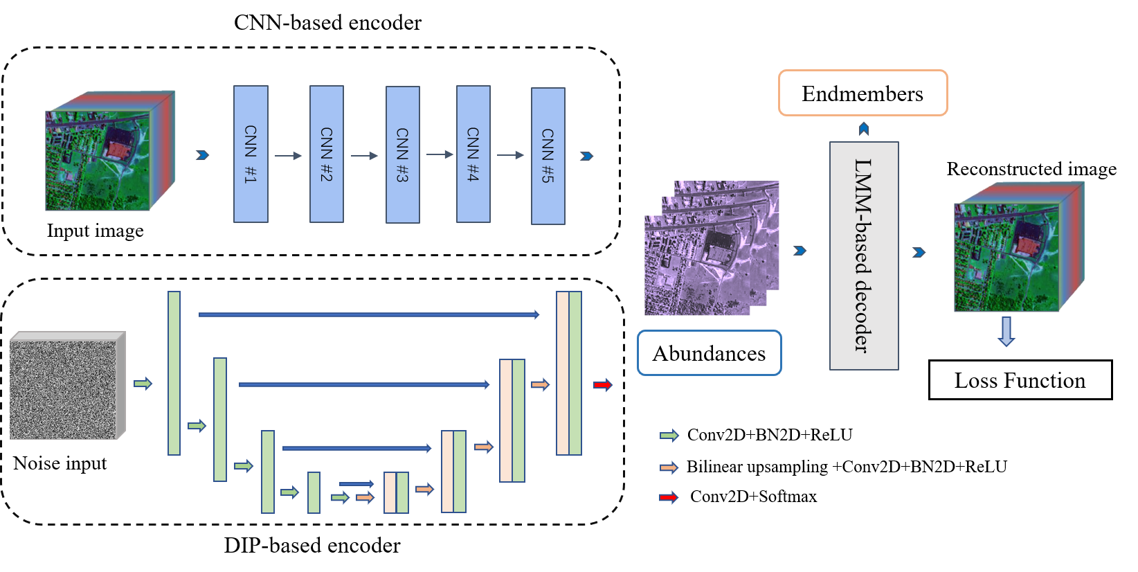
Figure 2: The architectures of CNN-based and DIP-based networks used as particular instances of the proposed method.

IV-B Updating $\bm{\Theta}$

At each iteration, the set of parameters $\bm{\Theta}$ of the autoencoder is updated through rule (9). This can be achieved by training the network with the function in (9) as the objective function. The first term measures the data fit while the second acts as a regularization to enforce the representation $\mathsf{E}_{\bm{\Theta}_{\sf E}}(\mathbf{W})$ in the latent space to be close to a corrected version $\mathbf{A}-\mathbf{G}$ of the abundance. Regarding the ASC, ANC and ENC constraints, they can be ensured by an appropriate design of the network. In practice, Adam is used to train the autoencoder.

Various autoencoder architectures can be envisioned and the encoder and the decoder can be chosen by the end-user with respect to the targeted applicative context. The encoder $\mathsf{E}_{\bm{\Theta}_{\sf E}}(\cdot)$ aims at extracting relevant features to be incorporated into the estimated abundances. A popular choice is a CNN-based architecture where the input is the observed image. Another promising approach consists in leveraging on a deep image prior (DIP) with a noise input. These two particular choices are discussed later in this section. Regarding the decoder $\mathsf{D}_{\bm{\Theta}_{\sf D}}(\cdot)$, it generally mimics the mixing process and the endmembers usually define the weights of one specially designed linear layer. Again, the proposed AE-RED framework is sufficiently flexible to host various architectures and to handle various spectral mixing models. A popular strategy is to design the decoder such that it combines physics-based and data-driven strategies to account for complex nonlinearities or spectral variabilities. For instance, additive nonlinear and post-nonlinear models have been extensively investigated [32, 31, 35] as well as spectral variability-aware endmember generators [36, 37].

Some archetypal examples of possible elements composing the architecture of the AE are (non-exhaustively) listed in Fig. 1(c). In the sequel of this paper, for illustration purpose but without loss of generality, two particular architectures are discussed and then instantiated, as shown in Fig. 2. Both consider an LMM-based decoder composed of a convolutional layer with a filter size of $1\times 1\times B$ to mimic the LMM. The adjusted decoder weights are finally extracted to estimate the endmember spectral signature. For this particular instance of the decoder, the optimization problem (9) can be rewritten as

$$\left\{\bm{\Theta}_{\sf E},\mathbf{S}\right\} \in\arg\min_{\bm{\Theta}_{\sf E},\mathbf{S}}\|\mathbf{Y}-\mathbf{S}\mathsf{E}_{\bm{\Theta}_{\sf E}}(\mathbf{W})\|_{\text{F}}^{2}$$ (12)

$$+\mu\|\mathbf{A}-\mathsf{E}_{\bm{\Theta}_{\sf E}}(\mathbf{W})-\mathbf{G}\|_{\text{F}}^{2}$$

s.t. $$\ \bm{1}^{\top}_{R}\mathsf{E}_{\bm{\Theta}_{\sf E}}(\mathbf{W})=\bm{1}_{N}^{\top},~{}\mathsf{E}_{\bm{\Theta}_{\sf E}}(\mathbf{W})\geq\bm{0}~{}\text{and}~{}\mathbf{S}\geq\bm{0}.$$

The two examples of AE considered in this paper differ by the architecture of the encoder. The first network is composed of a CNN-based encoder while the second is a DIP. These two choices are discussed below.

IV-B1 CNN-based encoder

The architecture of the CNN-based encoder is shown in Fig. 2. The whole image $\mathbf{Y}$ is used here as the input to extract the structure information from the hyperspectral image. Another choice would consist in considering over-lapping patches as the input. The encoder is composed of 5 blocks. The first two blocks implement $3\times 3$ convolution filters to learn the spatial consistency information. The next two blocks apply $1\times 1$ convolution operators (i.e., fully connected layers) to model the spectral priors. Moreover, to satisfy the ANC and ASC, the conventional LeakyReLU activation function of the last block is replaced by a softmax function. The output dimensions of each block are narrowly diminished to compress the input pixels into the abundance domain. Considering the optimization function defined in (12), the objective function to train this model is expressed as

$$\mathcal{L}_{\text{AE}}(\bm{\Theta})=\|\mathbf{Y}-\mathbf{S}\mathsf{E}_{\bm{\Theta}_{\sf E}}(\mathbf{Y})\|_{\text{F}}^{2}+\mu\|\mathbf{A}-\mathsf{E}_{\bm{\Theta}_{\sf E}}(\mathbf{Y})-\mathbf{G}\|_{\text{F}}^{2}.$$ (13)

The resulting unmixing method will be denoted as AE-RED-C in the sequel.

IV-B2 Deep image prior-based encoder

Another architecture considered in this paper exploits the DIP strategy to implicitly learn the priors of hyperspectral image. Unlike conventional AE-based unmixing methods which use spectral signatures as input for training, this network applies a Gaussian noise image $\mathbf{Z}$ of size of the abundance matrix $\mathbf{A}$ as input to generate the hyperspectral image. The encoder can be a U-net like architecture to extract the features from different levels. In this work the encoder has been designed with an encoder-decoder structure for abundance estimation. The inner encoder is composed of 4 down-sampling to compress the features. Each down-sampling block consists of three layers, namely a convolution layer with a filter of size $3\times 3$, a batch normalization layer, and a ReLU nonlinear activation layer. The inner decoder is composed of 5 up-sampling blocks. Each of the first 4 blocks has 4 layers: a bilinear upsampling layer, a convolution layer, a batch normalization layer and a ReLU nonlinear activation layer. The last block has two layers, namely a convolution layer and a softmax nonlinear activation layer to generate the estimated abundances while satisfying the ANC and ASC. Skip connections relate the encoder and decoder which are used to fuse the low-level and high-level features and to obtain multiscale information. The objective function to train this deep model is also defined as (13) where $\mathsf{E}_{\bm{\Theta}_{\sf E}}(\mathbf{Y})$ is replaced by $\mathsf{E}_{\bm{\Theta}_{\sf E}}(\mathbf{Z})$. The proposed method with this architecture is denoted as AE-RED-U.

IV-C Updating $\mathbf{A}$

The abundance matrix $\mathbf{A}$ is updated by solving (10). This problem is a standard RED objective function and can be interpreted as a denoising of $\mathsf{E}_{\bm{\Theta}_{\sf E}}(\mathbf{W})+\mathbf{G}$. The seminal paper [42] discusses two algorithmic schemes to solve this problem, namely fixed-point and gradient-descent strategies. In this work we derive a fixed-point algorithm by setting the gradient of the objective function to $\bm{0}$,

$$\lambda\left(\mathbf{A}-\mathsf{C}\left(\mathbf{A}\right)\right)+\mu\left(\mathbf{A}-\mathsf{E}_{\bm{\Theta}_{\sf E}}(\mathbf{W})-\mathbf{G}\right)=\bm{0}.$$ (14)

Then, at the $(k+1)$th iteration of the ADMM, the $j$th inner iteration of the fixed-point algorithm can be summarized as

$$\mathbf{A}^{(k+1,j+1)}\\ =\frac{1}{\lambda+\mu}\left[\lambda\mathsf{C}\left(\mathbf{A}^{(k+1,j)}\right)+\mu\left(\mathsf{E}^{(k+1)}_{\bm{\Theta}_{\sf E}}(\mathbf{W})+\mathbf{G}^{(k)}\right)\right].$$ (15)

For illustration, we consider two particular denoisers $\mathsf{C}\left(\cdot\right)$, namely nonlocal means (NLM) [43] and block-matching and 4-D filtering (BM4D) [44]. NLM is a 2D denoiser and should be applied on each spectral bands indendently while and BM4D is a 3D-cube based denoiser. Depending on the architecture chosen for the encoder (see Section IV-B), the corresponding instances of the proposed framework are named as AE-RED-CNLM, AE-RED-CBM4D, AE-RED-UNLM and AE-RED-UBM4D, respectively.

Algorithm 1 The proposed unmixing framework AE-RED

1:Hyperspectal image $\mathbf{Y}$; Regularization parameter $\lambda$; ADMM coefficient $\mu$; Denoiser $\mathsf{C}(\cdot)$; Outer and inner iteration numbers $K$ and $J$; Training parameters (learning rate, epochs, batch size).

2:% ADMM iterations

3:for $k=1,\cdots,K$ do

4:% Updating $\bm{\Theta}$

5:   for $i=1,\cdots,\textrm{epochs}$ do

6:      Update $\mathsf{E}_{\bm{\Theta}_{\sf E}}(\mathbf{W})$ via forward propagation,

7:      Compute the loss function by (13),

8:      Update $\bm{\Theta}^{(k)}$ via retropropagation,

9:   end for

10:% Updating $\mathbf{A}$

11:   Set $\mathbf{A}^{(k-1,0)}=\mathbf{A}^{(k-1)}$

12:   for $j=1,\cdots,J$  do

13:      Update $\mathbf{A}^{(k-1,j)}$ with (15),

14:   end for

15:   Set $\mathbf{A}^{(k)}=\mathbf{A}^{(k-1,J)}$

16:% Updating $\mathbf{G}$

17:   Update $\mathbf{G}^{(k)}$ with (11);

18:end for

19:Estimated abundances $\mathbf{A}$ and endmembers $\mathbf{S}$.

V Experimental results

This section presents experiments conducted to evaluate the effectiveness of the proposed unmixing framework. These experiments have been conducted on synthetic and real data sets to quantitatively assess the unmixing results and to demonstrate the effectiveness of our proposed method in real applications, respectively (see Sections V-A and V-B).

Compared methods – Several state-of-the-art methods have been compared. A first family of unmixing algorithms are conventional methods. SUnSAL-TV [16] leverages on a handcrafted TV-term to regularize the optimization function. PnP-NMF [9] is an NMF-based unmixing method, and denoisers are embedded as PnP to introduce prior information. A second family of compared methods is based on deep learning. CNNAE [10] is a deep AE-based unmixing method where convolutional filters capture spatial information. UnDIP [45] is a DIP-based unmixing method which uses a convolutional network. A geometric endmember extraction method is applied to estimate endmembers. SNMF [39] is a deep unrolling algorithm, which unfolds the $\ell_{p}$-sparsity constrained NMF model into trainable deep architectures. CyCU-Net [11] proposes a cascaded AEs for unmixing with a cycle-consistency loss to enhance the unmixing performance.

Hyperparameter settings – All hyperparameters of the compared methods have been manually adjusted to obtain the best unmixing performance. The choice of the parameters associated with the proposed AE-RED method are discussed in detail as follows. The regularization parameters $\lambda$ and $\mu$ have been selected according to the noise level of generated data. More precisely, $\lambda$ and $\mu$ have been set to $0.5$ for the data with noise levels of $5$dB and $10$dB, to $0.1$ for the data with a noise level of $20$dB, to $0.01$ for the data with a noise level of $30$dB. The learning rate to train the deep networks is set to $1\times 10^{-3}$, and set $1\times 10^{-4}$ to fine-tune the decoder weights. For the proposed CNN based unmixing method, the number $K$ of ADMM iterations is set to $15$, the number of epochs is set to $250$ and the number of inner iterations when updating the abundances is set to $J=1$. As for the proposed DIP based unmixing method, $K$, the number of epochs and $J$ are respectively set to $10$, $2300$ and $1$.

Performance metrics – The root mean square error (RMSE) is used to evaluate the abundance estimation performance, which can be expressed by

$$\text{RMSE}=\sqrt{\frac{1}{NR}\sum_{i=1}^{N}\|\mathbf{a}_{i}-\hat{\mathbf{a}}_{i}\|^{2}},$$ (16)

where $\mathbf{a}_{i}$ is the actual abundance of the $i$th pixel, and $\hat{\mathbf{a}}_{i}$ is the corresponding estimate. A smaller value of RMSE indicates better abundance estimation results. The endmember estimation is assessed by computing the mean spectral angle distance (mSAD) and the mean spectral information divergence (mSID) given by

$$\text{mSAD}=\frac{1}{R}\sum_{r=1}^{R}\arccos\left(\frac{\mathbf{s}_{r}^{\top}\hat{\mathbf{s}}_{r}}{\|\mathbf{s}_{r}\|\|\hat{\mathbf{s}}_{r}\|}\right)$$ (17)

and

$$\text{mSID}=\frac{1}{R}\sum_{r=1}^{R}\mathbf{p}_{r}\log\left(\frac{\mathbf{p}_{r}}{\hat{\mathbf{p}}_{r}}\right),$$ (18)

where $\mathbf{s}_{r}$ and $\hat{\mathbf{s}}_{r}$ are the actual and estimate of the $r$th endmember, respectively, $\mathbf{p}_{r}={\mathbf{s}_{r}}/{\bm{1}^{\top}\mathbf{s}_{r}}$ and $\hat{\mathbf{p}}_{i}={\hat{\mathbf{s}}_{r}}/{\bm{1}^{\top}\hat{\mathbf{s}}_{r}}$. A smaller value indicates better estimation results. Finally, the peak signal-to-noise ratio (PSNR) is used to evaluate the image denoising and reconstruction, which is defined by

$$\text{PSNR}=10\times\log_{10}\left(\frac{\text{MAX}^{2}}{\text{MSE}}\right)$$ (19)

where MAX is the maximum pixel value of the reconstructed image $\hat{\mathbf{Y}}$ and MSE is the mean square error between the reconstructed image and the noise-free image. A higher value of PSNR indicates better reconstruction.

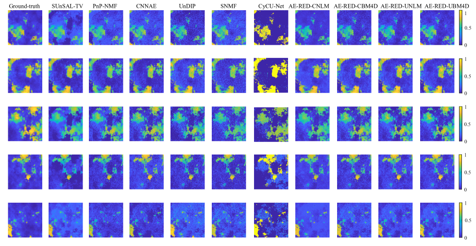
Figure 3: Synthetic data, SNR$=10$dB: estimated abundance maps.

TABLE II: synthetic data: performance (in term of RMSE) of the abundance estimation. Best RMSEs are reported in bold and underlined numbers denote the second best RMSEs.

	$5$dB	$10$dB	$20$dB	$30$dB
SUnSAL-TV	0.1112	0.0804	0.0284	0.0104
PnP-NMF	0.1029	0.0711	0.0311	0.0117
CNNAE	0.1078	0.0682	0.0292	0.0127
UnDIP	0.1469	0.0854	0.0280	0.0100
SNMF	0.1207	0.0906	0.0313	0.0112
CyCU-Net	0.1150	0.0708	0.0296	0.0139
AE-RED-CNLM	0.0943	0.0640	0.0261	0.0097
AE-RED-CBM4D	0.1009	0.0665	0.0235	0.0093
AE-RED-UNLM	0.0919	0.0602	0.0241	0.0095
AE-RED-UBM4D	0.0972	0.0585	0.0251	0.0094

TABLE III: Synthetic data: performance (in term of mSAD) of the endmember estimation. Best mSADs are reported in bold and underlined numbers denote the second best mSADs.

	$5$dB	$10$dB	$20$dB	$30$dB
SUnSAL-TV	0.1013	0.0623	0.0173	0.0052
PnP-NMF	0.0855	0.0533	0.0181	0.0083
CNNAE	0.0811	0.0481	0.0162	0.0045
UnDIP	0.0977	0.0685	0.0193	0.0057
SNMF	0.0852	0.0595	0.0113	0.0043
CyCU-Net	0.0826	0.0569	0.0146	0.0069
AE-RED-CNLM	0.0769	0.0437	0.0103	0.0041
AE-RED-CBM4D	0.0770	0.0430	0.0105	0.0042
AE-RED-UNLM	0.0767	0.0434	0.0108	0.0040
AE-RED-UBM4D	0.0768	0.0433	0.0107	0.0039

TABLE IV: Synthetic data: performance (in term of mSID) of the endmember estimation. Best mSIDs are reported in bold and underlined numbers denote the second best mSIDs.

	$5$dB	$10$dB	$20$dB	$30$dB
SUnSAL-TV	0.0391	0.0120	0.0013	0.0002
PnP-NMF	0.0195	0.0100	0.0011	0.0002
CNNAE	0.0432	0.0069	0.0013	0.0003
UnDIP	0.0650	0.0130	0.0023	0.0001
SNMF	0.1369	0.0112	0.0007	0.0001
CyCU-Net	0.0447	0.0052	0.0014	0.0003
AE-RED-CNLM	0.0184	0.0038	0.0005	0.0001
AE-RED-CBM4D	0.0189	0.0036	0.0006	0.0001
AE-RED-UNLM	0.0195	0.0037	0.0007	0.0001
AE-RED-UBM4D	0.0187	0.0037	0.0006	0.0001

TABLE V: Synthetic data: performance (in term of PSNR) of the image reconstruction. Best PSNRs are reported in bold and underlined numbers denote the second best PSNRs.

	$5$dB	$10$dB	$20$dB	$30$dB
SUnSAL-TV	30.8279	35.3531	43.9418	54.4288
PnP-NMF	31.6765	36.2873	44.3496	54.6453
CNNAE	31.4510	35.2500	43.3465	50.9367
UnDIP	30.3016	34.8235	44.3141	54.6996
SNMF	28.1358	32.2243	41.2482	51.3990
CyCU-Net	30.8153	35.4829	42.6938	50.1539
AE-RED-CNLM	32.4931	36.8916	44.4119	54.7001
AE-RED-CBM4D	31.7141	36.1305	45.3226	54.8153
AE-RED-UNLM	32.0177	36.6815	44.4916	55.0293
AE-RED-UBM4D	32.2841	36.9038	44.5306	55.2367

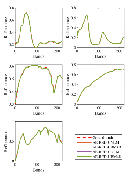
Figure 4: Estimated endmembers of synthetic data (SNR = 20 dB).

V-A Experiments on the Synthetic data set

Data description – The synthetic images are composed of $100\times 100$ pixels. Abundance maps are generated using the method of the Hyperspectral Imagery Synthesis tools to mimic a spatial homogeneity. A Gaussian field is drawn to generate the abundance matrix $\mathbf{A}$. The abundance ground-truth is shown in Fig. 3. The abundances maps satisfy ANC and ASC. Sets of $R=5$ endmembers are randomly selected from the U.S. Geological Survey (USGS) spectral library with a number of spectral bands of $B=224$. These endmembers are mixed according to the LMM and an additive zero-mean Gaussian noise is considered with variances according to $4$ signal-to-noise (SNR) ratios, i.e., $\mathrm{SNR}\in\left\{5\mathrm{dB},10\mathrm{dB},20\mathrm{dB},30\mathrm{dB}\right\}$.

Results – Tables II-V report the estimation results obtained by the compared algorithms in terms of RMSE for the abundance estimation, mSAD and mSID for the endmember estimation and PSNR for the reconstruction. Conventional unmixing methods, such as SUnSAL-TV and PnP-NMF, achieve good unmixing results, demonstrating the usefulness of the explicit prior provided by manually designed regularization. Deep learning-based methods, such as CNNAE, SNMF and CyCU-Net, they can obtain suitable unmixing results and better endmember estimation results compared with the conventional methods, illustrating the ability of deep networks of embedding prior information. These results also show that the proposed AE-RED framework outperforms the compared state-of-the-art methods, across all performance metrics and the noise levels. Fig. 3 depicts the estimated abundance maps associated with the synthetic data set with SNR$=10$dB. It can be observed that the abundance maps estimated by the AE-RED framework exhibit better agreement with the ground-truth. Fig. 4 shows the endmember estimated by the proposed framework on the synthetic data set with SNR$=20$dB, which are consistent with the ground-truth.

V-B Experiments on the Real data set

Data description – Finally, experiments conducted on two real data sets are discussed. Firstly, one considers the Samson data set, which was acquired by SAMSON observer and contains $B=156$ spectral channels ranging from $400$ nm to $889$ nm. The original image is of size of $952\times 952$ pixels, and a subimage of $95\times 95$ pixels is cropped in the experiment. There are three endmembers in this data, namely “water”, “tree” and “soil”. The second real data set used in these experiments is known as the Jasper Ridge image. It was acquired by Analytical Imaging and Geophysics (AIG) in 1999 with $B=224$ spectral bands covering a spectral range from $380$ nm to $2500$ nm. One considers a subimage of size of $100\times 100$ pixels and $B=198$ channels after removing the bands affected by water vapor and atmospheric effects. It contains $R=4$ endmembers, namely “water”, “soil”, “tree” and “road”.

TABLE VI: Samson and Jasper Ridge data sets: performance comparison in term of PSNR. Best results are reported in bold and underlined numbers denote the second best results.

	SUnSAL-TV	PnP-NMF	CNNAE	UnDIP	SNMF	CyCU-Net	AE-RED-CNLM	AE-RED-CBM4D	AE-RED-UNLM	AE-RED-UBM4D
Samson	32.6306	35.2650	28.6785	36.2918	29.7175	31.1702	35.6806	35.3954	35.5137	35.4009
Jasper Ridge	31.1325	29.2783	24.9619	32.1480	28.8746	28.7161	31.3895	30.0416	31.6140	30.0416

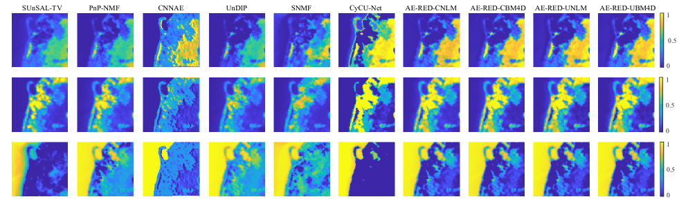
Figure 5: Samson data set: estimated abundance maps.

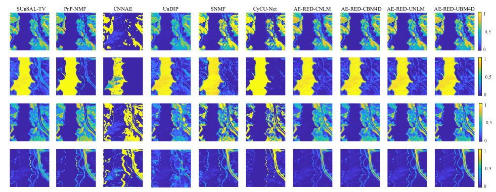
Figure 6: Jasper Ridge data set: estimated abundance maps

Results – As there is no available ground-truth for real datasets, a quantitative performance evaluation of abundances and endmembers cannot be provided. Therefore, we only rely on PSNR to evaluate the results of the compared methods. Table VI presents the PSNR performance associated with the compared methods obtained on the Samson data set. It is noteworthy that all methods produce comparable PSNR results, except for CNNAE, SNMF, and CyCU-Net, which provide significantly worse reconstruction. Although there is no ground-truth for the abundances, we can visually inspect the maps. For illustration purposes, we show the abundance maps estimated by the compared methods in Fig. 5. The proposed AE-RED framework can successfully separate the materials and provide sharp abundance estimates.

Table VI also lists the PSNR results for the Jasper Ridge data set. It can also be observed that the proposed method reaches the best PSNR. Fig. 6 depicts the abundance maps estimated by all compared methods. Some of them, such as UnDIP, fail to recover the road. Due to the learning ability of deep networks, most deep learning based methods are able distinguish the individual materials. Finally the proposed AE-RED framework provides abundance maps with more detailed information and sharper boundaries.

VI Conclusion

This paper proposed a generic unmixing framework to embed a RED within an autoencoder. By carefully designing the encoder and the decoder, the autoencoder was able to provide estimated abundance maps and endmember spectra. In particular, for illustration purpose, two different encoder architectures are considered, namely a CNN and a DIP. Moreover the decoder could be chosen according to a particular mixture model. Leveraging on ADMM scheme, the resulting optimization problem was split into simpler subproblems. The first one was described by an objective function composed of a data-fitting term and a quadratic regularization. It was solved through the training of an autoencoder. The second subproblem was a standard RED objective function and solved by the fixed-point strategy. Two denoisers were considered, namely NLM and BM4D. The effectiveness of the proposed framework was evaluated through experiments conducted on synthetic and real data sets. The results showed that the proposed framework outperformed state-of-the-art methods. Future works include considering explicit endmember priors within the proposed framework and automatically selecting mixing model.

References

- [1] N. Dobigeon, L. Tits, B. Somers, Y. Altmann, and P. Coppin, “A comparison of nonlinear mixing models for vegetated areas using simulated and real hyperspectral data,” IEEE J. Sel. Topics Appl. Earth Observations Remote Sensing, vol. 7, no. 6, pp. 1869–1878, June 2014.
- [2] P. W. Yuen and M. Richardson, “An introduction to hyperspectral imaging and its application for security, surveillance and target acquisition,” The Imaging Science Journal, vol. 58, no. 5, pp. 241–253, 2010.
- [3] Y. Duan, H. Huang, and T. Wang, “Semisupervised feature extraction of hyperspectral image using nonlinear geodesic sparse hypergraphs,” IEEE Trans. Geosci. Remote Sens., 2021.
- [4] F. Luo, L. Zhang, B. Du, and L. Zhang, “Dimensionality reduction with enhanced hybrid-graph discriminant learning for hyperspectral image classification,” IEEE Trans. Geosci. Remote Sens., vol. 58, no. 8, pp. 5336–5353, 2020.
- [5] J. M. Bioucas-Dias, A. Plaza, G. Camps-Valls, P. Scheunders, N. Nasrabadi, and J. Chanussot, “Hyperspectral remote sensing data analysis and future challenges,” IEEE Geosci. Remote Sens. Mag., vol. 1, no. 2, pp. 6–36, 2013.
- [6] N. Dobigeon, J.-Y. Tourneret, C. Richard, J. C. M. Bermudez, S. McLaughlin, and A. O. Hero, “Nonlinear unmixing of hyperspectral images: Models and algorithms,” IEEE Signal Proc. Mag., vol. 31, no. 1, pp. 82–94, 2013.
- [7] R. A. Borsoi, T. Imbiriba, J. C. M. Bermudez, C. Richard, J. Chanussot, L. Drumetz, J.-Y. Tourneret, A. Zare, and C. Jutten, “Spectral variability in hyperspectral data unmixing: A comprehensive review,” IEEE Geosci. Remote Sens. Mag., vol. 9, no. 4, pp. 223–270, 2021.
- [8] L. Dong, Y. Yuan, and X. Luxs, “Spectral–spatial joint sparse NMF for hyperspectral unmixing,” IEEE Trans. Geosci. Remote Sens., vol. 59, no. 3, pp. 2391–2402, 2020.
- [9] M. Zhao, T. Gao, J. Chen, and W. Chen, “Hyperspectral unmixing via nonnegative matrix factorization with handcrafted and learned priors,” IEEE Geoscience and Remote Sensing Letters, vol. 19, pp. 1–5, 2021.
- [10] B. Palsson, M. O. Ulfarsson, and J. R. Sveinsson, “Convolutional autoencoder for spectral–spatial hyperspectral unmixing,” IEEE Trans. Geosci. Remote Sens., vol. 59, no. 1, pp. 535–549, 2020.
- [11] L. Gao, Z. Han, D. Hong, B. Zhang, and J. Chanussot, “CyCU-Net: Cycle-consistency unmixing network by learning cascaded autoencoders,” IEEE Trans. Geosci. Remote Sens., 2021.
- [12] S. Ozkan, B. Kaya, and G. B. Akar, “Endnet: Sparse autoencoder network for endmember extraction and hyperspectral unmixing,” IEEE Trans. Geosci. Remote Sens., vol. 57, no. 1, pp. 482–496, 2018.
- [13] L. Miao and H. Qi, “Endmember extraction from highly mixed data using minimum volume constrained nonnegative matrix factorization,” IEEE Trans. Geosci. Remote Sens., vol. 45, no. 3, pp. 765–777, 2007.
- [14] M.-D. Iordache, J. M. Bioucas-Dias, and A. Plaza, “Collaborative sparse regression for hyperspectral unmixing,” IEEE Trans. Geosci. Remote Sens., vol. 52, no. 1, pp. 341–354, 2013.
- [15] P. V. Giampouras, K. E. Themelis, A. A. Rontogiannis, and K. D. Koutroumbas, “Simultaneously sparse and low-rank abundance matrix estimation for hyperspectral image unmixing,” IEEE Trans. Geosci. Remote Sens., vol. 54, no. 8, pp. 4775–4789, 2016.
- [16] M.-D. Iordache, J. M. Bioucas-Dias, and A. Plaza, “Total variation spatial regularization for sparse hyperspectral unmixing,” IEEE Trans. Geosci. Remote Sens., vol. 50, no. 11, pp. 4484–4502, 2012.
- [17] A. Halimi, Y. Altmann, N. Dobigeon, and J.-Y. Tourneret, “Nonlinear unmixing of hyperspectral images using a generalized bilinear model,” IEEE Trans. Geosci. Remote Sens., vol. 49, no. 11, pp. 4153–4162, 2011.
- [18] J. Chen, M. Zhao, X. Wang, C. Richard, and S. Rahardja, “Integration of physics-based and data-driven models for hyperspectral image unmixing: A summary of current methods,” IEEE Signal Proc. Mag., vol. 40, no. 2, pp. 61–74, 2023.
- [19] X. Zhang, Y. Yuan, and X. Li, “Sparse unmixing based on adaptive loss minimization,” IEEE Trans. Geosci. Remote Sens., vol. 60, pp. 1–14, 2022.
- [20] J. Peng, W. Sun, H.-C. Li, W. Li, X. Meng, C. Ge, and Q. Du, “Low-rank and sparse representation for hyperspectral image processing: A review,” IEEE Geosci. Remote Sens. Mag., 2021.
- [21] D. P. Kingma and J. Ba, “Adam: A method for stochastic optimization,” arXiv preprint arXiv:1412.6980, 2014.
- [22] I. Sutskever, J. Martens, G. Dahl, and G. Hinton, “On the importance of initialization and momentum in deep learning,” in International conference on machine learning. PMLR, 2013, pp. 1139–1147.
- [23] J. Sigurdsson, M. O. Ulfarsson, and J. R. Sveinsson, “Hyperspectral unmixing with regularization,” IEEE Trans. Geosci. Remote Sens., vol. 52, no. 11, pp. 6793–6806, 2014.
- [24] Y. Zhong, R. Feng, and L. Zhang, “Non-local sparse unmixing for hyperspectral remote sensing imagery,” IEEE J. Sel. Top. Appl. Earth Observat. Remote Sens., vol. 7, no. 6, pp. 1889–1909, 2013.
- [25] X. Wang, Y. Zhong, L. Zhang, and Y. Xu, “Spatial group sparsity regularized nonnegative matrix factorization for hyperspectral unmixing,” IEEE Trans. Geosci. Remote Sens., vol. 55, no. 11, pp. 6287–6304, 2017.
- [26] A. Lagrange, M. Fauvel, S. May, and N. Dobigeon, “Matrix cofactorization for joint spatial–spectral unmixing of hyperspectral images,” IEEE Trans. Geosci. Remote Sens., vol. 58, no. 7, pp. 4915–4927, 2020.
- [27] L. Tong, J. Zhou, B. Qian, J. Yu, and C. Xiao, “Adaptive graph regularized multilayer nonnegative matrix factorization for hyperspectral unmixing,” IEEE J. Sel. Top. Appl. Earth Observat. Remote Sens., vol. 13, pp. 434–447, 2020.
- [28] M. Zhao, X. Wang, J. Chen, and W. Chen, “A plug-and-play priors framework for hyperspectral unmixing,” IEEE Trans. Geosci. Remote Sens., vol. 60, pp. 1–13, 2021.
- [29] Z. Wang, L. Zhuang, L. Gao, A. Marinoni, B. Zhang, and M. K. Ng, “Hyperspectral nonlinear unmixing by using plug-and-play prior for abundance maps,” Remote Sensing, vol. 12, no. 24, p. 4117, 2020.
- [30] Y. Qu and H. Qi, “uDAS: An untied denoising autoencoder with sparsity for spectral unmixing,” IEEE Trans. Geosci. Remote Sens., vol. 57, no. 3, pp. 1698–1712, 2018.
- [31] M. Zhao, L. Yan, and J. Chen, “LSTM-DNN based autoencoder network for nonlinear hyperspectral image unmixing,” IEEE J. Sel. Top. Sig. Process., vol. 15, no. 2, pp. 295–309, 2021.
- [32] M. Zhao, M. Wang, J. Chen, and S. Rahardja, “Hyperspectral unmixing for additive nonlinear models with a 3-D-CNN autoencoder network,” IEEE Trans. Geosci. Remote Sens., vol. 60, pp. 1–15, 2021.
- [33] Z. Hua, X. Li, Y. Feng, and L. Zhao, “Dual branch autoencoder network for spectral-spatial hyperspectral unmixing,” IEEE Geosci. Remote Sens. Lett., vol. 19, pp. 1–5, 2021.
- [34] M. Wang, M. Zhao, J. Chen, and R. Susanto, “Nonlinear unmixing of hyperspectral data via deep autoencoder network,” IEEE Geosci. Remote Sens. Lett., pp. 1–5, 2019.
- [35] K. T. Shahid and I. D. Schizas, “Unsupervised hyperspectral unmixing via nonlinear autoencoders,” IEEE Trans. Geosci. Remote Sens., vol. 60, pp. 1–13, 2021.
- [36] R. Borsoi, T. Imbiriba, and J. Bermudez, “Deep generative endmember modeling: An application to unsupervised spectral unmixing,” IEEE Trans. Comput. Imag., vol. 6, pp. 374–384, 2019.
- [37] S. Shi, M. Zhao, L. Zhang, Y. Altmann, and J. Chen, “Probabilistic generative model for hyperspectral unmixing accounting for endmember variability,” IEEE Trans. Geosci. Remote Sens., vol. 60, 2022.
- [38] Y. Qian, F. Xiong, Q. Qian, and J. Zhou, “Spectral mixture model inspired network architectures for hyperspectral unmixing,” IEEE Trans. Geosci. Remote Sens., vol. 58, no. 10, pp. 7418–7434, 2020.
- [39] F. Xiong, J. Zhou, S. Tao, J. Lu, and Y. Qian, “SNMF-Net: Learning a deep alternating neural network for hyperspectral unmixing,” IEEE Trans. Geosci. Remote Sens., vol. 60, pp. 1–16, 2021.
- [40] Z. Lai, K. Wei, and Y. Fu, “Deep plug-and-play prior for hyperspectral image restoration,” Neurocomputing, vol. 481, pp. 281–293, 2022.
- [41] R. Dian, S. Li, and X. Kang, “Regularizing hyperspectral and multispectral image fusion by CNN denoiser,” IEEE transactions on neural networks and learning systems, vol. 32, no. 3, pp. 1124–1135, 2020.
- [42] Y. Romano, M. Elad, and P. Milanfar, “The little engine that could: Regularization by denoising (RED),” SIAM Journal on Imaging Sciences, vol. 10, no. 4, pp. 1804–1844, 2017.
- [43] A. Buades, B. Coll, and J.-M. Morel, “Non-local means denoising,” Image Processing On Line, vol. 1, pp. 208–212, 2011.
- [44] M. Maggioni, V. Katkovnik, K. Egiazarian, and A. Foi, “Nonlocal transform-domain filter for volumetric data denoising and reconstruction,” IEEE Trans. Image Process., vol. 22, no. 1, pp. 119–133, 2012.
- [45] B. Rasti, B. Koirala, P. Scheunders, and P. Ghamisi, “UnDIP: Hyperspectral unmixing using deep image prior,” IEEE Trans. Geosci. Remote Sens., vol. 60, pp. 1–15, 2021.