Bootstrapping the Cross-Validation Estimate

Abstract

Cross-validation is a widely used technique for evaluating the performance of prediction models. It helps avoid the optimism bias in error estimates, which can be significant for models built using complex statistical learning algorithms. However, since the cross-validation estimate is a random value dependent on observed data, it is essential to accurately quantify the uncertainty associated with the estimate. This is especially important when comparing the performance of two models using cross-validation, as one must determine whether differences in error estimates are a result of chance fluctuations. Although various methods have been developed for making inferences on cross-validation estimates, they often have many limitations, such as stringent model assumptions This paper proposes a fast bootstrap method that quickly estimates the standard error of the cross-validation estimate and produces valid confidence intervals for a population parameter measuring average model performance. Our method overcomes the computational challenge inherent in bootstrapping the cross-validation estimate by estimating the variance component within a random effects model. It is just as flexible as the cross-validation procedure itself. To showcase the effectiveness of our approach, we employ comprehensive simulations and real data analysis across three diverse applications.

Keywords: random effects model, mean absolute prediction error, c-index, individualized treatment response score

1 Introduction

Predictive modeling has emerged as a prominent tool in biomedical research, encompassing diverse applications such as disease diagnosis, patient risk stratification, and personalized treatment recommendations, as seen in studies such as [25, 13, 24, 17]. A wide range of methods have been employed to create prediction models, from basic linear regression to sophisticated deep learning algorithms. Once the models have been developed, it’s crucial to assess their performance for a number of reasons. Firstly, the results from a model cannot be effectively utilized or interpreted without understanding its accuracy. For instance, a positive result from a model with a positive predictive value (PPV) of 20% will be treated differently from a positive result with a PPV of 1% by both physicians and patients. Secondly, with a wealth of prediction tools at hand, choosing the best model from a set of models can be a challenge, with multiple factors influencing the decision, including cost, interpretability, and, most importantly, the model’s future performance in a population. This performance can be measured in various ways, depending on the intended application of the model. If the model aims to predict clinical outcomes, its accuracy can be measured by a prediction accuracy metric, such as mean squared prediction error for continuous outcomes or a receiver operating characteristics (ROC) curve for classification. In other cases, the performance measure can be more complex. If the model is used to recommend treatment to individual patients, the model performance can be measured by the observed treatment benefit among patients who are recommended to receive a particular treatment according to the model. Lastly, even in the model construction step, evaluating the model performance is often needed for optimal tuning. For example, in applying neural networks, the network structure needs to be specified by the analyst to have best prediction performance.

Cross-validation is a commonly used technique to assess the performance of a predictive model and overcome the over-optimistic bias that results from using the same data for both training and evaluating the model [9, 12, 29, 21]. The approach involves using out-of-sample observations to evaluate model performance, thus avoiding optimism bias. The resulting cross-validation estimator is a random quantity, dependent on both the random splitting of data into training and testing sets, and the observed data itself. To reduce the randomness due to the splitting of data, one can repeat the training and testing process multiple times and average the prediction performance on the testing data. The randomness inherent in the observed data reflects the fact that if a new set of data were randomly sampled from the underlying population, the cross-validation results would be different from those based on the current observed data. In essence, the cross-validation estimator is a statistic, or a function of random data, despite its complex construction.

Realizing this fact, it is important to derive and estimate the distribution of this statistic so that we may (1) understand what population parameter the cross-validation procedure estimates and (2) attach an appropriate uncertainty measure to the cross-validation estimate [3, 20, 34]. For the simple case of large sample size and small number of parameters, the asymptotic distribution of the cross-validation estimator has been studied in depth [8, 27, 15, 19]. For example, when the model training and validation are based on the same loss function, the cross-validation estimator is asymptotically Gaussian [8]. A computationally efficient variance estimator for the cross-validated area under the ROC curve has also been proposed, if the parameters used in the classifier are estimated at the root $n$ rate [19]. More recently, Bayle et al. have established the asymptotic normality of general $K$-fold cross-validated prediction error estimates and proposed a consistent variance estimator under a set of stability conditions [3]. The learning algorithm can be general and flexible, but the error estimate in the validation set needs to be in the form of sum of identically independent distributed random elements. The validity of their proposed variance estimate requires that the variation from model training is dominated by that in estimating the prediction error in the testing set. Along a similar line, Austern and Zhou (2020) have also studied the asymptotic distribution of $K$ fold cross-validation estimates allowing $K$ increases with the sample size [1]. The proposed variance estimator is very similar to that in [3]. Asymptotic normality of the cross-validation estimator has been established when the prediction model is trained on the same loss as is used for evaluation, the same case as in [8]. A nested cross-validation method has been introduced to automatically quantify the uncertainty of the cross-validation estimate and construct confidence intervals for the model performance [2]. The key is to use an additional loop of cross-validations to correct the finite-sample bias of the variance estimator proposed in [3, 1]. However, this method still requires specific forms for the performance measure of interest and may not be applicable in certain applications.

The majority of previous work on cross-validation assumes a simpler form for the performance measure, such as the average of a random variable, and requires that the prediction model is trained using the same loss function. However, there are applications of cross-validation not covered by these conventional approaches, as demonstrated in Example 3 of the paper. Additionally, the validity of the proposed confidence intervals relies on suitable stability conditions and large sample approximations. Although resampling methods are a well-known approach for estimating the variance of a statistic and can provide fairly accurate approximations even with small to moderate sample sizes, the main challenge with using them in this setting is the computational speed. This paper aims to characterize the underlying population parameter estimated by the cross-validation procedure and to propose a general, computationally efficient resampling method for constructing a confidence interval for this population parameter, removing as many restrictions as possible.

2 Method

In a very general setup, we use random vector $X$ to denote individual observations, and the observed data consist of $n$ independent identically distributed (i.i.d.) copies of $X$, i.e., $D=\{X_{1},\cdots,X_{n}\}.$ The output of the training procedure is a parameter estimate, which can be a finite dimensional vector or infinite dimensional functions, denoted by $\hat{\psi}(D)$ to emphasize its dependence on observed data $D$ and the fact that it is a random quantity. In evaluating the “performance” of $\hat{\psi}(D)$ in a new testing set consisting of $m$ i.i.d. observations $\widetilde{D}=\{\widetilde{X}_{1},\cdots,\widetilde{X}_{m}\},$ a summary statistic is calculated as a function of testing data and $\hat{\psi}(D),$ which can be written as

$$L\left\{\widetilde{D},\hat{\psi}(D)\right\}.$$

It is possible to make inference and derive confidence interval on $L\left\{\widetilde{D},\hat{\psi}(D)\right\}$ by treating $\widetilde{D}$ or both $D$ and $\widetilde{D}$ as random. In most applications, however, we only have a single dataset, and the cross-validation procedure is needed in order to objectively evaluate the model performance. Specifically, In cross-validation, we randomly divide the observed data $D$ into two non-overlapping parts denoted by $D_{train}$ and $D_{test}$, and calculate $L\left\{D_{test},\hat{\psi}(D_{train})\right\}.$ In order to reduce the variability of random splits, the aforementioned step is oftentimes repeated many times and the average performance measure is obtained as the final cross-validation estimator of the model performance:

$$\widehat{Err}^{CV}=\frac{1}{B_{CV}}\sum_{b=1}^{B_{CV}}L\left\{D_{test}^{b},\hat{\psi}(D_{train}^{b})\right\},$$

where $D=D_{train}^{b}\cup D_{test}^{b}$ represents the $b$th split. The number of replications, $B_{CV}$, needs to be relatively large to reduce the Monte-Carlo variation due to random splits. It is often in the range of several hundreds in practice. Note that although we used $Err$ to represent the model performance in consistent with notations used in the literature [2], the performance measure is not necessarily a prediction error. It can be other metric with a higher value indicating a good performance as discussed in the following sections.

2.1 Applications

Many cross-validation applications can fit into the very general framework described above. In this paper, we will focus on several typical examples.

2.1.1 Application 1

In the first example, we are interested in evaluating the performance of predicting continuous outcomes measured by mean absolute prediction error [27, 32]. The result can help us to determine, for example, whether a newly developed prediction algorithm significantly outperform an existing model. The prediction model can be constructed by fitting a standard linear regression model, i.e., calculating a regression coefficient vector $\hat{\beta}(D_{train})$ by minimizing a $L_{2}$ loss function

$$\sum_{X_{i}\in D_{train}}\left(Y_{i}-\beta^{\prime}\widetilde{Z}_{i}\right)^{2},$$

based on a training dataset $D_{train}$, where $Z_{i}$ is the baseline covariate for the $i$th patient and $\widetilde{Z}_{i}=(1,Z_{i}^{\prime})^{\prime}$ including an intercept. If nonlinear prediction models are considered, then one may construct the prediction model via a more flexible machine learning algorithm such as random forest or neural network. In all cases, the prediction error in a testing set $D_{test}$ is calculated as

$$\hat{\theta}(D_{train},D_{test})=\frac{1}{n_{test}}\sum_{X_{i}\in D_{test}}|Y_{i}-\hat{\beta}(D_{train})^{\prime}\tilde{Z}_{i}|,$$

where $n_{test}$ is the number of observations in the testing set. In cross-validation, we may repeatedly split an observed dataset $D$ into training and testing sets of given sizes, $(D_{train},D_{test})$ , and obtain the corresponding cross-validated mean absolute prediction error estimator, $\hat{\theta}(D_{train},D_{test})$. In the end, the sample average of those resulting cross-validated mean absolute prediction error estimators becomes the final estimator measuring the predictive performance of the linear model. In this application, $X=(Z,Y)$ with $Z$ and $Y$ being the predictor and outcome of interest, respectively, $\hat{\psi}(D)=\hat{\beta}(D)$, and the summary statistic measuring the prediction performance is:

$$L\left(D_{test},\psi\right)=\frac{1}{n_{test}}\sum_{X_{i}\in D_{test}}|Y_{i}-\psi^{\prime}\widetilde{Z}_{i}|.$$

2.1.2 Application 2

In the second example, we are interested in evaluating the performance of a prediction model in predicting binary outcomes by its c-index for new patients, which is the area under the ROC curve [11, 23]. The result can help us to determine, for example, whether c-index from a new prediction model is significantly higher than 0.5 or a desirable level. The prediction model can be constructed via fitting a logistic regression model, i.e., calculating a regression coefficient vector $\hat{\beta}(D_{train})$ by maximizing the log-likelihood function

$$\sum_{(Z_{i},Y_{i})\in D_{train}}\left[\beta^{\prime}Z_{i}Y_{i}-\log\left\{1+\exp(\beta^{\prime}\tilde{Z}_{i})\right\}\right],$$

based on a training dataset $D_{train}$. If the dimension of the predictor $Z_{i}$ is high, a lasso-regularization can be employed in estimating $\beta$. In any case, a concordance measure, the c-index in a testing set $D_{test}$ can be calculated as

$$\hat{\theta}(D_{train},D_{test})=\frac{1}{\tilde{n}_{test,0}\tilde{n}_{test,1}}\sum_{X_{i}\in D_{test}(0)}\sum_{X_{j}\in D_{test1}(1)}I\left(\hat{\beta}(D_{train})^{\prime}\tilde{Z}_{i}<\hat{\beta}(D_{train})^{\prime}\tilde{Z}_{j}\right),$$

where $\tilde{n}_{test,g}$ is the number of observations in the set $D_{test}(g)=\{(Z_{i},Y_{i})\in D_{test}:Y_{i}=g\},g\in\{0,1\}.$ In cross-validation, we may repeatedly split the observed dataset $D$ into training and testing sets, $(D_{train},D_{test}),$ and obtain the corresponding cross-validated c-indexes $\hat{\theta}(D_{train},D_{test})$. In the end, the sample average of those resulting cross-validated c-index estimator is our final estimator measuring the classification performance of the logistic regression. In this application, $X=(Z,Y)$ with $Z$ and $Y$ being the predictor and a binary outcome of interest, respectively, $\hat{\psi}(D)=\hat{\beta}(D)$, and

$$L\left(D_{test},\psi\right)=\frac{1}{\tilde{n}_{test,0}\tilde{n}_{test,1}}\sum_{X_{i}\in D_{test}(0)}\sum_{X_{j}\in D_{test}(1)}I\left(\psi^{\prime}\tilde{Z}_{i}<\psi^{\prime}\tilde{Z}_{j}\right).$$

Remark 1

In evaluating the performance of the logistic regression model for predicting binary outcomes, we may choose to use the entire ROC curve to measure the model performance. Since the construction of a stable ROC curve requires sufficient number of cases, i.e, observations with $Y_{i}=1,$ and controls, i.e., observations with $Y_{i}=0,$ one may want to construct the ROC curve with as many observations from testing set as possible. In particular, one can implement the $K$-fold cross-validation, i.e., randomly splitting the observed dataset $D$ in to $K$ parts of approximately equal sizes: $D=D_{1}\cup D_{2}\cup\cdots D_{K}.$ Let $\hat{\beta}(D^{(-k)})$ be the regression coefficient estimated based on observations not in the $k$th part of the observed data. We may then construct the predicted risk score for patients in the $k$th part as $\hat{\beta}(D^{(-k)})^{\prime}Z_{i}.$ Cycling through $k=1,\cdots,K,$ we can obtain a predicted risk score for every patient as

$$\hat{R}_{i}({\cal D})=\left\{\sum_{k=1}^{K}\hat{\beta}(D^{(-k)})I(X_{i}\in D_{k})\right\}^{\prime}Z_{i},i=1,\cdots,n,$$

where ${\cal D}$ represents the particular division of the observed dataset into $K$ parts. The ROC curve can then be calculated as

$$\widehat{ROC}(u\mid{\cal D})=\hat{S}_{1{\cal D}}\left\{\hat{S}_{0{\cal D}}^{-1}(u)\right\},$$

where $\hat{S}_{g{\cal D}}(\cdot)$ is the empirical survival function of $\left\{\hat{R}_{i}({\cal D})\mid Y_{i}=g,i=1,\cdots,n\right\},g\in\{0,1\},$ depending on the particular division of ${\cal D}$. In cross-validation, we may repeatedly split the observed dataset $D$ into $K$ parts and obtain the corresponding cross-validated ROC curve $\widehat{ROC}(u\mid{\cal D})$, and the sample average of those resulting ROC curves becomes the final estimator of the ROC curve measuring the predictive performance of the logistic regression. In this example,

$$L\left(D_{test},\psi\right)(u)=\hat{S}_{1}\left\{\hat{S}_{0}^{-1}(u\mid\psi,D_{test})\mid\psi,D_{test}\right\},$$

where $\hat{S}_{g}(\cdot\mid\psi,D_{test})$ is empirical survival function of $\left\{\psi^{\prime}Z_{i}\mid Y_{i}=g,X_{i}\in D_{test}\right\},g\in\{0,1\}.$ Our proposed method will cover inference for estimator from $K$ fold cross-validation as well.

2.1.3 Application 3

In the third example, we are interested in developing a precision medicine strategy and evaluating its performance in a randomized control setting. Specifically, the precision medicine strategy here is a binary classification rule to recommend a treatment to a patient based on his or her baseline characteristics to maximize the treatment benefit for individual patient as well as in a patient population of interest. Before applying this recommendation to clinical practice, it is important to estimate the uncertainty of the treatment effect in the identified subgroup who would be recommended for the treatment, to make sure the anticipated stronger treatment effect is real. There are many different ways of constructing such a treatment recommendation classifier [5, 26]. For example, one may first construct a individualized treatment response (ITR) score by minimizing a loss function based on a training dataset $D_{train},$

$$\sum_{X_{i}\in D_{train}}\left\{Y_{i}-\gamma^{\prime}\tilde{Z}_{i}-(G_{i}-\pi)\beta^{\prime}\tilde{Z}_{i}\right\}^{2},$$

where $X_{i}=(Z_{i},G_{i},Y_{i}),$ $Y_{i}$ is the response of interest with a higher value being desirable, $G_{i}\in\{0,1\}$ is a binary treatment indicator and independent of the baseline covariate $Z_{i}$ (i.e., the treatment is randomly assigned to patients in the training set), and $\pi=P(G_{i}=1).$ Let the resulting minimizers of $\gamma$ and $\beta$ be $\hat{\gamma}(D_{train})$ and $\hat{\beta}(D_{train})$, respectively [26, 33]. Note that we have the decomposition that

$$E\left\{\left(Y-\gamma^{\prime}\tilde{Z}-(G-\pi)\beta^{\prime}\tilde{Z}\right)^{2}\right\}$$

$$= P(G=1)E\left\{\left(Y^{(1)}-\gamma^{\prime}\tilde{Z}-(1-\pi)\beta^{\prime}\tilde{Z}\right)^{2}\right\}+P(G=0)E\left\{\left(Y^{(0)}-\gamma^{\prime}\tilde{Z}+\pi\beta^{\prime}\tilde{Z}\right)^{2}\right\}$$

$$= E\left[\left(Y-\gamma^{\prime}\tilde{Z}\right)^{2}+\pi(1-\pi)\left(Y^{(1)}-Y^{(0)}-\beta^{\prime}\tilde{Z}\right)^{2}-\pi(1-\pi)\left(Y^{(1)}-Y^{(0)}\right)^{2}\right],$$

where $Y^{(g)}$ is the potential outcome if the patient receives treatment $g\in\{0,1\},$ and the observed outcome $Y=Y^{(1)}G+Y^{(0)}(1-G).$ Therefore, minimizing the original loss function with respect to $\beta$ amounts to approximating the conditional average treatment effect (CATE),

$$\Delta(z)=E\left(Y^{(1)}-Y^{(0)}\mid Z=z\right),$$

via $(1,z^{\prime})\hat{\beta}(D_{train})$, a linear function of $Z=z$, because the solution $\widehat{\beta}(D_{train})$ minimizes a loss function, whose population limit is

$$E\left\{\left(Y^{(1)}-Y^{(0)}-\beta^{\prime}\tilde{Z}\right)^{2}\right\}.$$

The constructed ITR score is $\widehat{\Delta}(z\mid D_{train})=(1,z^{\prime})\hat{\beta}(D_{train}),$ which can be used to guide the treatment recommendation for individual patient. There are other ways of constructing the ITR score approximating the CATE. Once an estimated ITR score is available, one may recommend treatment $G=1$ to patients whose $\widehat{\Delta}(Z\mid D_{train})>c_{0}$ and treatment $G=0$ to patients whose $\widehat{\Delta}(Z\mid D_{train})\leq c_{0},$ where $c_{0}$ is a constant reflecting the “cost” of the treatment. Here, we choose $c_{0}=0$ for simplicity. In the testing set, one may evaluate the performance of this recommendation system by estimating the average treatment effect among the subgroup of patients recommended to receive the treatment $G=1,$ i.e, $\widehat{D}_{test}^{(1)}=\left\{X\in D_{test}\mid\widehat{\Delta}(Z\mid D_{train})>0\right\}$ and among the subgroup of patients recommended to receive the treatment $G=0,$ i.e., $\widehat{D}_{test}^{(0)}=\left\{X\in\widehat{D}_{test}\mid\widehat{\Delta}(Z\mid D_{train})\leq 0\right\}.$ Specifically, we may consider the observed treatment effects

$$\widehat{\Delta}_{1}(D_{train},D_{test})=\frac{\sum_{X_{i}\in\hat{D}_{test}^{(1)}}Y_{i}G_{i}}{\sum_{X_{i}\in\hat{D}_{test}^{(1)}}G_{i}}-\frac{\sum_{X_{i}\in\hat{D}_{test}^{(1)}}Y_{i}(1-G_{i})}{\sum_{X_{i}\in\hat{D}_{test}^{(1)}}(1-G_{i})}$$

and

$$\widehat{\Delta}_{0}(D_{train},D_{test})=\frac{\sum_{X_{i}\in\hat{D}_{test}^{(0)}}Y_{i}G_{i}}{\sum_{X_{i}\in\hat{D}_{test}^{(0)}}G_{i}}-\frac{\sum_{X_{i}\in\hat{D}_{test}^{(0)}}Y_{i}(1-G_{i})}{\sum_{X_{i}\in\hat{D}_{test}^{(0)}}(1-G_{i})}$$

If $\widehat{\Delta}_{1}(D_{train},D_{test})$ takes a “large” positive value and $\widehat{\Delta}_{0}(D_{train},D_{test})$ takes a “large” negative value, (in other words, the treatment effect is indeed estimated to be greater among those who are recommended to receive the treatment based on the constructed ITR score), then we may conclude that $\widehat{\Delta}(Z\mid D_{train})>0,$ is an effective treatment recommendation system. In cross-validation, we may repeatedly divide the observed data set $D$ into training and testing sets, $(D_{train},D_{test}),$ and obtain the corresponding cross-validated treatment effect difference $\widehat{\Delta}_{g}(D_{train},D_{test}),g\in\{0,1\}$. In the end, the sample average of those resulting cross-validated treatment effect estimators is our final cross-validation estimator measuring the performance of the treatment recommendation system. In this application $X=(Z,G,Y)$ with $Z$, $G$ and $Y$ being predictors, treatment assignment indicator, and a binary outcome, respectively, $\hat{\psi}(D)=\hat{\beta}(D)$, and

$$L\left(D_{test},\psi\right)=\frac{\sum_{X_{i}\in D_{test}}Y_{i}G_{i}I(\psi^{\prime}Z_{i}>0)}{\sum_{X_{i}\in D_{test}}G_{i}I(\psi^{\prime}Z_{i}>0)}-\frac{\sum_{X_{i}\in D_{test}}Y_{i}(1-G_{i})I(\psi^{\prime}Z_{i}>0)}{\sum_{X_{i}\in D_{test}}(1-G_{i})I(\psi^{\prime}Z_{i}>0)}$$

or

$$~{}~{}~{}~{}~{}~{}~{}~{}~{}~{}~{}~{}~{}~{}~{}~{}~{}~{}~{}\frac{\sum_{X_{i}\in D_{test}}Y_{i}G_{i}I(\psi^{\prime}Z_{i}\leq 0)}{\sum_{X_{i}\in D_{test}}G_{i}I(\psi^{\prime}Z_{i}\leq 0)}-\frac{\sum_{X_{i}\in D_{test}}Y_{i}(1-G_{i})I(\psi^{\prime}Z_{i}\leq 0)}{\sum_{X_{i}\in D_{test}}(1-G_{i})I(\psi^{\prime}Z_{i}\leq 0)}.$$

2.2 The Estimand of Cross-validation

The first important question is what population parameter the cross-validation procedure estimates. As discussed in [2], there are several possibilities. The first obvious population parameter is

$$Err(D_{n})=\lim_{N\rightarrow\infty}L\left(\tilde{D}_{N},\hat{\psi}(D_{n})\right),$$

where $D_{n}$ is the training set of sample size $n$ and $\tilde{D}_{N}$ is a new independent testing set of sample size $N$ drawing from the same distribution as the training dataset, $D_{n}$. This parameter depends on the training set $D_{n},$ and directly measures the performance of the prediction model obtained from observed data $D_{n}$ in a future population. The second population parameter of interest is

$$Err_{n}=E\{Err(D_{n})\},$$

the average performance of prediction models trained based on “all possible” training sets of size $n$ sampled from the same distribution as the observed dataset, $D_{n}.$ The subscript $n$ emphasizes the fact that this population parameter only depends on the sample size of the training set $D_{n}.$ While $Err(D_{n})$ is the relevant parameter of interest in most applications, where we want to know the future performance of the prediction model at hand, $Err_{n}$ is a population parameter reflecting the expected performance of prediction models trained via a given procedure. The prediction performance of the model from the observed dataset $D_{n}$ can be better or worse than this expected average performance. It is known that the cross-validation targets on evaluating a training procedure rather than the particular prediction model obtained from the training procedure. Specifically, the cross-validation estimator $\widehat{Err}^{CV}_{m}$ actually estimates $Err_{m}$ in the sense that

$$\left(\begin{array}[]{c}\widehat{Err}_{m}^{CV}\\ Err(D_{n})\end{array}\right)\approx\left(\begin{array}[]{c}Err_{m}+\epsilon\\ Err_{n}+\zeta\end{array}\right),$$

where $m$ is the sample size of the training set used in constructing the cross-validation estimate, i.e., the dataset $D_{n}$ is repeatedly divided into a training set of size $m$ and a testing set of size $(n-m)$ in cross-validation. Here, $\epsilon$ and $\zeta$ are two mean zero random noises and oftentimes nearly independent. In many cases $Err_{n}\approx Err_{m}$, when $m$ is not substantially smaller than $n.$ If we ignore their differences, then $\widehat{Err}^{CV}_{m}$ can also be viewed as an approximately unbiased estimator for $Err(D_{n})$, because

$$\widehat{Err}^{CV}_{m}-Err(D_{n})=(Err_{m}-Err_{n})+(\epsilon-\zeta),$$

whose mean is approximately zero. On the other hand, the variance of $\widehat{Err}^{CV}_{m}-Err(D_{n})$ tends to be substantially larger than the variance of $\widehat{Err}^{CV}_{m}-Err_{m},$ since $\epsilon$ and $\zeta$ are often independent and the variance of $\zeta$ is nontrivial relative to that of $\epsilon$. This is analogous to the phenomenon that the sample mean of observed data is a natural estimator of the population mean. It also can be viewed as an unbiased “estimator” of the sample mean of a set of future observations, because the expectation of sample mean of future observations is the same as the population mean, which can be estimated by the sample mean of observed data. In this paper, we take $Err_{m}$ as the population parameter of interest, because approximately $Err(D_{n})$ is simply $Err_{m}$ plus a random noise $\zeta$, which may be independent of the cross-validation estimate. In other words, we take the view that the cross-validation estimate evaluates the average performance of a training procedure rather than the performance of a particular prediction model. As the training sample size goes to infinity, we write $Err=\lim_{n\rightarrow\infty}Err_{n}.$ When $n$ is sufficiently large, $Err\approx Err_{n}\approx Err(D_{n}).$

In the following, we use a simple example to demonstrate the relationship of aforementioned quantities.

2.2.1 A Toy Example

Consider the linear prediction model in section 2.1.1. Suppose that covariate $Z_{i}\sim N(0,I_{10})$, and the response $Y_{i}=\alpha_{0}+\beta_{0}^{\prime}Z_{i}+\epsilon_{i},i=1,\cdots,n,$ where $I_{10}$ is 10 by 10 identity matrix, $\alpha_{0}=0$, $\beta_{0}=(1,1,1,1,0,0,0,0,0,0)^{\prime},$ $\epsilon_{i}\sim N(0,1)$ and $n=90.$ We were interested in constructing a prediction model via fitting a linear regression model and evaluating its performance in terms of the mean absolute prediction error. To this end, for each simulated dataset $D_{n}=\{X_{i}=(Z_{i},Y_{i}),i=1,\cdots,n\},$ we estimated the regression coefficients of the linear model by ordinary least square method and denoted the estimators of $\alpha_{0}$ and $\beta_{0}$ by $\hat{\alpha}(D_{n})$ and $\hat{\beta}(D_{n}),$ respectively. Then we calculated the true mean absolute prediction error as the expectation of $|G|,$ where $G\sim N\left(\hat{\alpha}(D_{n}),1+\|\hat{\beta}(D_{n})-\beta_{0}\|_{2}^{2}\right)$ is a random variable. This expectation was $Err(D_{n})$, the prediction error of the model trained based on dataset $D_{n}$ in a future population. We also constructed the cross-validation estimate of the prediction error by repeatedly splitting $D_{n}$ into a training set of size $m=80$ and a testing set of size $n-m=10.$ The resulting estimator for the estimation error was $\widehat{Err}_{m}^{CV}.$ Repeating these steps, we obtained 1000 pairs of $Err(D_{n})$ and $\widehat{Err}_{m}^{CV}$ from simulated datasets. The empirical average of 1000 $Err(D_{n})$s was an approximation to $Err_{n}=E\left\{Err(D_{n})\right\}.$ Figure 1(a) is the scatter plot of $Err(D_{n})$ vs. $\widehat{Err}^{CV}_{m}$ based on 1000 simulated datasets. It was clear that $\widehat{Err}^{CV}_{m}$ and $Err(D_{n})$ were almost independent but shared a similar center. Specifically, the empirical average of $\widehat{Err}^{CV}_{m}$ was 0.859, and the empirical average of $Err(D_{n})$ was 0.851. Therefore, the cross-validated error estimator $\widehat{Err}^{CV}_{m}$ can be viewed as a sensible estimator for $Err_{n}=E\left\{Err(D_{n})\right\}\approx 0.851$, and more precisely an unbiased estimator for $Err_{m}$, whose value was estimated as 0.861 using the same simulation described above. Note that $(m,n)=(80,90)$ and $n$ and $m$ are fairly close. The distribution of the cross-validated error estimators along with $Err_{m}$ and $Err_{n}$ are plotted in Figure 1(b), suggesting that the small difference between $Err_{80}$ and $Err_{90}$ is negligible relative to the variation of the cross-validation estimator $\widehat{Err}^{CV}_{m}$ itself. In addition, $\widehat{Err}^{CV}_{m}$ can also be thought as a “prediction” to $Err(D_{n}),$ since the latter was approximately $Err_{n}$ plus an independent mean zero “measurement error”.

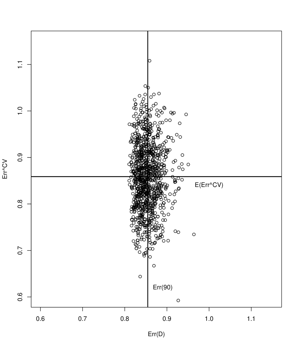
(a) $Err(D_{n})$ vs $\widehat{Err}^{CV}_{m}$ for estimating the mean absolute prediction error

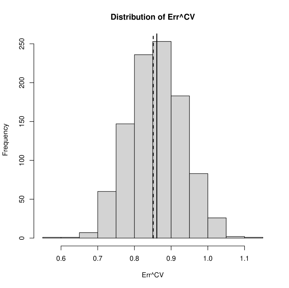
(b) The distribution of $\widehat{Err}^{CV}_{m}$ for estimating the mean absolute prediction error; $Err_{n}$: dashed line; $Err_{m}$: solid line

2.3 Statistical Inference on $Err_{m}$

In this section, we aim to construct a valid confidence interval for $Err_{m}$ based on the cross-validated estimate. First, we define the cross-validated estimate with repeated training and testing splits as

$$\widehat{Err}^{CV}_{m}=E\left[L\left\{D_{test}^{b},\hat{\psi}(D_{train}^{b})\right\}\right]$$

where the expectation is with respect to random division of training and testing sets. One may anticipate that $\widehat{Err}^{CV}$ is a “smooth” functional with respect to the empirical distribution of observed data $D_{n}$, because each individual observation’s contribution to the final estimator is “averaged” across different training and testing divisions. Therefore, we expect that $\widehat{Err}^{CV}_{m}$ is a root-$n$ regular estimator of $Err$, i.e.,

$$\sqrt{n}\left(\widehat{Err}^{CV}_{m}-Err\right)\rightarrow N(0,\sigma_{D}^{2}),$$

in distribution as $n$, the sample size of $D_{n}$, goes to infinity and $\lim_{n\rightarrow\infty}m/n\in(0,1).$ Indeed, under the following regularity conditions, this weak convergence holds in general.

1. $\hat{\psi}-\psi_{0}$ has a first order expansion, i.e,

   $$\hat{\psi}-\psi_{0}=\frac{1}{n}\sum_{i=1}^{n}\xi(X_{i})+o_{p}(n^{-1/2}),$$

   where $\hat{\psi}$ is a consistent estimator for a population parameter $\psi_{0}$ based on $D_{n}=\{X_{1},\cdots,X_{n}\},$ and $\xi(X_{i}),i=1,\cdots,n$ are independent mean zero random elements with a finite variance.

2. The process $L\left(D_{n},\psi\right)-E\left\{L(D_{n},\psi)\right\}$ is stochastic equal continuous at $\psi$, i.e.,

   $$\sqrt{n}\left[L\left(D_{n},\psi_{1}\right)-E\left\{L(D_{n},\psi_{1})\right\}\right]-\sqrt{n}\left[L\left(D_{n},\psi_{2}\right)-E\left\{L(D_{n},\psi_{2})\right\}\right]=o_{p}(1)$$

   as $\|\psi_{2}-\psi_{1}\|=o(1),$ where $\|\cdot\|$ is an appropriate norm measuring the distance between $\psi_{1}$ and $\psi_{2}.$ [16]

3. The random sequences

   $$\sqrt{n}\left[L\left(D_{n},\psi_{0}\right)-E\left\{L(D_{n},\psi_{0})\right\}\right]=\frac{1}{\sqrt{n}}\sum_{i=1}^{n}\eta(X_{i})+o_{p}(1),$$

   converges to a mean zero Gaussian distribution, where $\eta(X_{i})$ are independent mean zero random elements with a finite variance.

4. There exists a linear functional $l_{\psi}(\cdot)$ indexed by $\psi,$ such that

   $$E\left\{L(D_{n},\psi_{2})\right\}-E\left\{L(D_{n},\psi_{1})\right\}=l_{\psi_{1}}(\psi_{2}-\psi_{1})+o(\|\psi_{2}-\psi_{1}\|).$$

In the Appendix, we have provided an outline to show that

$$\sqrt{n}\left\{L\left\{D_{test}^{b},\hat{\psi}(D_{train}^{b})\right\}-Err\right\}$$

$$= \frac{1}{\sqrt{n}}\sum_{i=1}^{n}\left[\frac{I(X_{i}\in D_{test})}{1-\hat{\pi}}\eta(X_{i})+\frac{I(X_{i}\in D_{train})}{\hat{\pi}}l_{\psi_{0}}\{\xi(X_{i})\}\right]+o_{p}(1),$$

where $\hat{\pi}=m/n.$ After taking expectation with respect to the random training and testing division, i.e., indicators $\{I(X_{i}\in D_{train}),i=1,\cdots,n\},$

$$E\left\{\frac{I(X_{i}\in D_{test})}{1-\hat{\pi}}\right\}=E\left\{\frac{I(X_{i}\in D_{train})}{\hat{\pi}}\right\}=1$$

and

$$\sqrt{n}\left\{\widehat{Err}^{CV}_{m}-Err\right\}=\frac{1}{\sqrt{n}}\sum_{i=1}^{n}\left[\eta(X_{i})+l_{\psi_{n}}\{\xi(X_{i})\}\right]+o_{p}(1)$$

converges weakly to a mean zero Gaussian random distribution with a variance of

$$\sigma_{D}^{2}=E\left(\left[\eta(X)+l_{\psi_{0}}\{\xi(X)\}\right]^{2}\right).$$

For a finite sample $n$, we expect that the difference between $Err_{m}$ and $Err$ may be negligible. Specifically, the distribution of

$$\sqrt{n}\left(\widehat{Err}^{CV}_{m}-Err_{m}\right)$$

can be approximated by $N(0,\hat{\sigma}_{D}^{2}),$ if the following condition holds

1. $E\left[\lim_{N\rightarrow}\left\{L(D_{N},\widehat{\psi}_{n})\right\}\right]-Err=o_{p}(n^{-1/2}),$ where $\widehat{\psi}_{n}$ is based on training set of size $n,$ and the expectation is with respect to $\widehat{\psi}_{n}.$

This assumption is in general true, since $L(D_{N},\widehat{\psi}_{n})$ often converges to a smooth functional of $\widehat{\psi}_{n}$ as $N\rightarrow\infty,$ and the expectation of the limit can be approximated by $Err=\lim_{N\rightarrow}\left\{L(D_{N},\psi_{0})\right\}$ with the approximation error bounded by $O\left\{|E(\widehat{\psi}_{n}-\psi_{0})|\right\},$ which is in the order of $o(n^{-1/2})$ following condition C1. Since $E\left\{\widehat{Err}^{CV}_{m}\right\}$ is closer to $Err_{m}$ than $Err$ in finite sample setting, the Gaussian approximation for $\sqrt{n}\left(\widehat{Err}^{CV}_{m}-Err_{m}\right)$ is likely to be more accurate. As a consequence, an asymptotical confidence interval for $Err_{m}$ can be constructed as

$$\left[\widehat{Err}^{CV}_{m}-1.96\frac{\hat{\sigma}_{D}}{\sqrt{n}},\widehat{Err}^{CV}_{m}+1.96\frac{\hat{\sigma}_{D}}{\sqrt{n}}\right],$$

where $\hat{\sigma}_{D}$ is a consistent estimator of the standard error $\sigma_{D}.$ However, in general it is difficult to obtain such a consistent variance estimator when complex procedures such as lasso regularized regression or random forest are used for constructing the prediction model as in three examples discussed above. An appealing solution is to use the nonparametric bootstrap to estimate $\sigma_{D}^{2}$ [7, 10]. The rational is that, under the same set of assumptions,

$$\sqrt{n}\left\{\widehat{Err}^{CV*}_{m}-Err_{m}\right\}=\frac{1}{\sqrt{n}}\sum_{i=1}^{n}\left[\eta(X_{i})+l_{\psi_{0}}\{\xi(X_{i})\}\right]W_{i}+o_{P^{*}}(1),$$

where $\widehat{Err}^{CV*}_{m}$ is the cross-validated estimator based on bootstrapped data $D^{*}_{n}$, $(W_{1},\cdots,W_{n})\sim Multn\left(n,(1/n,\cdots,1/n)\right)$, $W_{i}$ is the number of observation $X_{i}$ in $D^{*}_{n},$ and $P^{*}$ is the product probability measure with respect to random data and the independent random weights $(W_{1},\cdots,W_{n}).$ Therefore, conditional on observed data $D_{n},$

$$\sqrt{n}\left\{\widehat{Err}^{CV*}_{m}-\widehat{Err}^{CV}_{m}\right\}=\frac{1}{\sqrt{n}}\sum_{i=1}^{n}\left[\eta(X_{i})+l_{\psi_{0}}\{\xi(X_{i})\}\right](W_{i}-1)+o_{P^{*}}(1),$$

converges weakly to a mean zero Gaussian distribution with a variance of

$$\hat{\sigma}^{2}_{D}=\frac{1}{n}\sum_{i=1}^{n}\left[\eta(X_{i})+l_{\psi_{0}}\{\xi(X_{i})\}\right]^{2}=\sigma_{D}^{2}+o_{P}(1).$$

Operationally, the following naive bootstrap procedure is expected to generate a consistent variance estimator of $\sigma_{D}^{2}$, $\hat{\sigma}_{D}^{2}.$

Algorithm 1 Naive Bootstrap

small

1:for $b\leftarrow 1$ to $B_{BOOT}$ do

2:     Sample original data to form a bootstrapped dataset of the size $n$ denoted by $D_{b}^{*};$

3:     Perform cross-validation based on bootstrapped dataset $D_{b}^{*};$

4:     for $k\leftarrow 1$ to $B_{CV}$ do

5:         Randomly split $D^{*}_{b}$ into $D^{*(k)}_{b,train}$ of size $m$ and $D^{*(k)}_{b,test}$ of size $n-m;$

6:         Calculate $L\left\{D_{b,test}^{*(k)},\hat{\psi}(D_{b,train}^{*(k)})\right\}$

7:     end for

8:     Calculate the bootstrapped cross-validation estimate

$$\widehat{Err}_{b,m}^{CV*}=\frac{1}{B_{CV}}\sum_{k=1}^{B_{CV}}L\left\{D_{b,test}^{*(k)},\hat{\psi}(D_{b,train}^{*(k)})\right\}.$$

9:end for

The variance $\sigma_{D}^{2}$ can be estimated by $n$ times the empirical variance of $B$ bootstrapped cross-validation estimates $\left\{\widehat{Err}_{1,m}^{CV*},\cdots,\widehat{Err}_{B_{BOOT},m}^{CV*}\right\}.$ However, there are several concerns in this naive resampling procedure, which may result in poor performance in practice.

• The bootstrap procedure samples observations with replacement and results in potential duplicates of the same observation in the bootstrapped dataset. Naively splitting the bootstrapped dataset into training and testing sets may result in overlap between them, which can induce nontrivial optimistic bias in evaluating the model performance. If we apply the naive bootstrap method to analyze the Toy Example described in section 2.2.1, then the empirical average of bootstrapped cross-validation estimates $\widehat{Err}_{b,m}^{CV*}$ was downward biased in comparison with $Err_{m}^{CV}$ by 0.80 standard deviation of cross-validation estimates $\widehat{Err}_{m}^{CV}.$ The practical influence of overlap on the variance estimation is less clear but can be potentially nontrivial.

• The training set of size $m$ in the bootstrapped dataset $D^{*}$ contains substantially fewer than $m$ distinct observations, which reduces the “effective” sample size for training a prediction model and induces a downward bias in evaluating the average model performance. This downward bias may be smaller or greater than the optimism bias induced by the overlap between training and testing sets depending on specific applications, but is undesirable in general.

• To obtain a cross-validated estimate for each bootstrap sample, one needs to perform the cross-validation multiple times to reduce the Monte-Carlo variation due to random training/testing divisions, i.e., $B_{CV}$ needs to be sufficiently big such as $\geq 200.$ In addition, the number of bootstraps also can not be too small. The conventional recommendation for estimating variance of a statistic using bootstrap is to set the number of bootstraps $B_{BOOT}\sim 400-1000.$ In such a case, one needs to train and evaluate the prediction model more than $80,000$ times and the corresponding computational burden can be prohibitive for complex training algorithm.

In this paper, we present a modified bootstrap procedure to overcome aforementioned difficulties.

First, in implementing cross-validation on a bootstrapped dataset, we view bootstrapped data as a weighted samples of the original data, i.e., observation $X_{i}$ is weighted by a random weight $W_{i}$, which is the number of this observation selected in this bootstrap iteration. In cross-validation, we first split the original dataset into training and testing sets, $D_{n}=D_{train}\cup D_{test},$ and bootstrapped training and testing sets denoted by $D^{*}_{train}$ and $D^{*}_{test}$, respectively, are then constructed by collecting all observations in $D_{train}$ and $D_{test},$ respectively, but with their respective bootstrap weights. Since $D_{train}$ and $D_{test}$ have no overlap, $D^{*}_{train}\cap D^{*}_{test}=\phi$ as well. Therefore, we don’t allow that the same observation used in both training and testing. One consequence is that the sample sizes of $D^{*}_{train}$ and $D^{*}_{test}$ are not fixed across different bootstrap samples. But their average sample sizes remain the same as those for $D_{train}$ and $D_{test}.$

Second, we note that the effective sample size of the training set based on the bootstrapped data can be substantially smaller than $m$. Specifically, the number of distinct observations in $D_{train}^{*}$ is $0.632m$ on average [9]. Therefore, it is desirable to increase the number of distinct observations of $D_{train}^{*}$ by allocating more observations to $D_{train}$, which is used to generate $D_{train}^{*}$ in a bootstrapped dataset. Ideally, we may want to increase the sample size of $D_{train}$ such that the number of distinct observations used for training is close to $m$ in bootstrapped cross-validation, i.e., $\#D_{train}^{*}\approx m,$ which requires to increase the sample size in $D_{train}$ from $m$ to $m/0.632.$ On the other hand, the sample size of $D_{test}$ and thus $D_{test}^{*}$ would be reduced by using a larger training set in the bootstrapped cross-validation and such a large reduction in testing sample size may increase the variance of the resulting estimate. In summary, while we want to increase the sample size in the training set to reduce the bias of estimating the model performance in bootstrapped cross-validation due to the fact that fewer distinct observations are used to train the prediction model, we also want to limit the reduction in the number of testing samples so that the variance of the cross-validation estimate would not be greatly affected by this adjustment in training and testing sample sizes. A compromise is to find a adjusted sample size $m_{adj}$ by minimizing the loss function

$$\left(\frac{m_{adj}}{0.632m}-1\right)^{2}+\lambda_{0}\left(\frac{n-m}{n-m_{adj}}-1\right)^{2},$$ (1)

where the first and second terms control the closeness of the “effective” sample size in the bootstrapped training set to $m$ and the relative change in the sample size of the testing set after the adjustment, respectively. Here, $\lambda_{0}$ controls the relative importance of theses two tasks in determining the final adjustment. In our limited experience, we have found that the performance of the resulting resampling procedure was not very sensitive to the selection of this penalty parameter within a wide range, and we recommended to set $\lambda_{0}=1-0.632=0.368$ in practice.

More importantly, to alleviate the computational demand for the bootstrap procedure, we propose the following algorithm:

Algorithm 2 Bootstrap Cross-Validation

1:for $b\leftarrow 1$ to $B_{BOOT}$ do

2:    Obtain a bootstrapped dataset $D^{*}_{b}$ and frequencies of all observations $\{W_{1b},\cdots,W_{nb}\}.$

3:    Calculate $m_{adj}$ by minimizing the loss function in (1) with $\lambda_{0}=0.368$;

4:    for $k\leftarrow 1$ to $B_{CV}$ do

5:         Split $D_{n}$ into training and testing sets: $D^{(k)}_{b,train}$ of size $m_{adj}$ and $D^{(k)}_{b,test}$ of size $n-m_{adj};$

6:         Construct the training and testing sets $D_{b,train}^{*(k)}$ and $D_{b,test}^{*(k)}$ by weighing patients in $D^{(k)}_{b,train}$ and $D^{(k)}_{b,test}$ with their bootstrap weights $\left\{W_{ib},i=1,\cdots,n\right\}.$

7:         Calculate the cross-validation error $\theta^{*}_{bk}=L\left\{D^{*(k)}_{b,train},D^{*(k)}_{b,test}\right\}$

8:    end for

9:    Calculate the bootstrapped cross-validation estimate $\widehat{Err}_{b,m}^{CV*}=B_{CV}^{-1}\sum_{k=1}^{B_{CV}}\theta^{*}_{bk}.$

10:end for

11:Fit a random effects model [18]

$$\theta^{*}_{bk}=\theta_{0}+\epsilon^{*}_{b}+\epsilon_{bk},b=1,\cdots,B_{BOOT};k=1,\cdots,B_{CV}$$

where $\epsilon^{*}_{b}\sim N(0,\sigma_{BT}^{2})$ and $\epsilon_{bk}$ are independent mean zero noise with a variance of $\tau_{0}^{2}$.

12:Let

$$\widehat{\sigma}_{BT}^{2}=\frac{1}{B_{BOOT}-1}\sum_{b=1}^{B_{BOOT}}(\bar{\theta}^{*}_{b}-\bar{\theta}^{*})^{2}-\frac{1}{B_{CV}(B_{CV}-1)B_{BOOT}}\sum_{b=1}^{B_{BOOT}}\sum_{k=1}^{B_{CV}}(\theta^{*}_{bk}-\bar{\theta}^{*}_{b})^{2},$$

where $\bar{\theta}_{b}^{*}=B_{CV}^{-1}\sum_{k=1}^{B_{CV}}\theta^{*}_{bk}$ and $\bar{\theta}^{*}=B_{BOOT}^{-1}\sum_{b=1}^{B_{BOOT}}\bar{\theta}^{*}_{b}.$

13:$\widehat{\sigma}_{m}^{CV}\leftarrow\widehat{\sigma}_{BT}$ is our bootstrap standard error estimator of cross-validation estimator $\widehat{Err}^{CV}_{m}$ and the 95% CI for $Err_{m}$ is

$$\left[\widehat{Err}^{CV}_{m}-1.96\times\widehat{\sigma}_{m}^{CV},\widehat{Err}^{CV}_{m}+1.96\times\widehat{\sigma}_{m}^{CV}\right].$$

The rational is that the center of $\theta^{*}_{bk}$, $\theta_{0}+\epsilon_{b}^{*},$ is approximately the cross-validation estimate based on the bootstrapped dataset $D^{*}_{b}$ as the number of random training and testing division increasing to infinity. Under this framework, $\sigma_{BT}^{2}$ measures the between-bootstrap variance, which is the bootstrap variance estimator we aim to calculate, and $\tau_{0}^{2}$ measures the within-bootstrap variance, i.e., the variance due to random training and testing divisions. The empirical variance of $\left\{\bar{\theta}^{*}_{1},\cdots,\bar{\theta}^{*}_{B}\right\}$ based on a very big $B_{CV}$ is approximately unbiased in approximating $\sigma_{BT}^{2},$ corresponding to the naive bootstrap procedure. However, this naive approach is very inefficient and there is no need to choose a very large $B_{CV}$ for eliminating the Monte-Carlo variance in estimating cross-validation prediction error for every bootstrapped dataset. Alternatively, an accurate moment estimate for the variance component in the random effects model can be constructed with a moderate $B_{CV}$, say $10-20,$ and a reasonably large $B_{BOOT},$ say 400. This can substantially reduce the computational burden from 80,000 model training to 8,000 model training.

Remark 2

The total number of model training is $B_{BOOT}\times B_{CV}.$ A natural question is how to efficiently allocate the number of bootstraps and number of cross-validations per bootstrap given the total number of model training. The variance estimator, $\hat{\sigma}_{BT}^{2},$ is a random statistic itself with a variance [4, 31], which can be approximated by

$$2\left(\frac{\left(\hat{\sigma}_{BT}^{2}+B_{CV}^{-1}\hat{\tau}_{0}^{2}\right)^{2}}{(B_{BOOT}-1)}\right)+2\left(\frac{\left(B_{CV}^{-1}\hat{\tau}_{0}^{2}\right)^{2}}{B_{BOOT}(B_{CV}-1)}\right),$$

where

$$\hat{\tau}_{0}^{2}=\frac{1}{B_{BOOT}(B_{CV}-1)}\sum_{b=1}^{B_{BOOT}}\sum_{k=1}^{B_{CV}}(\theta^{*}_{bk}-\bar{\theta}^{*}_{b})^{2}$$

is an estimator for $\tau_{0}^{2}.$ It is not difficult to show that fixing $B_{BOOT}\times B_{CV}=N_{T}$, the variance is minimized when

$$B_{BOOT}\approx\frac{\hat{\sigma}^{2}_{BT}}{\hat{\tau}^{2}_{0}}\times N_{T}$$

and

$$B_{CV}\approx\frac{\hat{\tau}^{2}_{0}}{\hat{\sigma}^{2}_{BT}}.$$

It suggests that the optimal number of cross-validation per bootstrap should be approximately constant, whose value may depend on the specific problem but doesn’t change with the budget for the total number of model training. Normally, $\hat{\tau}^{2}_{0}$ can be substantially greater than $\hat{\sigma}_{BT}^{2}$ and $B_{CV}$ should be set to be close to their ratio. In the toy example, this ratio is approximately 20. On the other hand, we always can increase the number of bootstraps to improve the precision in approximating the bootstrap variance estimator.

Remark 3

The number of distinct observations used in training the bootstrapped prediction model is smaller than $m_{adj}$. Specifically, the number of distinct observations in bootstrapped training set is on average only $0.632\times m_{adj}.$ Therefore, there is a tendency that the “effective total sample size” in bootstrap procedure is smaller than $n,$ which may cause a upward bias in estimating the variance of $\widehat{Err}_{m}^{CV}$ using the bootstrap variance estimator $\hat{\sigma}_{BT}^{2}.$ To correct this bias, we can consider an adjusted variance estimator

$$\left(\hat{\sigma}_{m,adj}^{CV}\right)^{2}=\hat{\sigma}_{BT}^{2}\left(\frac{n-m_{adj}+0.632m_{adj}}{n}\right)=\hat{\sigma}_{BT}^{2}\left(\frac{n-0.368m_{adj}}{n}\right),$$

where the factor $(n-0.368m_{adj})/n$ is introduced to account for the reduced sample size in bootstrapped training set. Note that we do not recommend a similar adjustment of the sample size in the testing set, even though that the number of distinct observations in the testing set is also smaller than $(n-m_{adj})$ in bootstrap, because in general this reduction in the number of distinct observations doesn’t affect the variance estimation.

Sometimes, training the prediction model can be very expensive in terms of computation, and it may not be feasible to conduct even the accelerated bootstrap. For example, one may only can train the prediction model 50-100 times. In such a case, regardless of the selection of $B_{BOOT}$ and $B_{CV}$, the Monte-Carlo error in estimating the bootstrap variance may not be ignorable. Consequentially,

$$\frac{\sqrt{n}(\widehat{Err}_{m}^{CV}-Err_{m})}{\widehat{\sigma}_{m}^{CV}}~{}~{}~{}\mbox{ or }~{}~{}~{}\frac{\sqrt{n}(\widehat{Err}_{m}^{CV}-Err_{m})}{\widehat{\sigma}_{m,adj}^{CV}}$$

may not follow a standard normal distribution. On the other hand, if we can empirically approximate this distribution, then one still can construct a 95% confidence interval for $Err_{m}$ based on $(\widehat{Err}_{m}^{CV},\widehat{\sigma}_{m}^{CV}).$ One analogy is that the confidence interval for the population mean of a normal distribution can be constructed using t-distribution rather than the normal distribution in small sample size setting. With a slight abuse of notations, let $\sigma_{m}^{CV}(\infty)$ be the bootstrap variance estimator, if both $B_{BOOT}$ and $B_{CV}\rightarrow\infty$, i.e., the bootstrap variance estimator without any Monte Carlo error, and we have

$$\frac{\sqrt{n}(\widehat{Err}_{m}^{CV}-Err_{m})}{\widehat{\sigma}_{m}^{CV}}=\frac{\sqrt{n}(\widehat{Err}_{m}^{CV}-Err_{m})}{\sigma_{m}^{CV}(\infty)}\times\frac{\sigma_{m}^{CV}(\infty)}{\widehat{\sigma}_{m}^{CV}}.$$ (2)

The first term of the left hand side of (2) should be approximated well by a standard Gaussian distribution since the “ideal” bootstrap variance estimator is used. The second term is independent of the first term and reflects the Monte-Carlo variation of approximating $\sigma_{m}^{CV}(\infty)$ via a small number of bootstrap and cross-validation iterations. To approximate the distribution of this ratio, we can bootstrap the variance estimator based on fitting the random effects model. This observation motivated the following additional steps presented in algorithm 3 after line (12-13) of algorithm 2, when very small $B_{BOOT}$ and $B_{CV}$ are used.

Algorithm 3 Bootstrap Calibration

13:for  $l\leftarrow 1$ to $L$ do

14:    Construct the bootstrapped dataset $\Theta_{l}^{*}=\left\{\theta^{**}_{lbk},b=1,\cdots,B_{BOOT};k=1,\cdots,B_{CV}\right\},$ where the vector $(\theta^{**}_{lb1},\cdots,\theta^{**}_{lbK})$ is a random sample from $B_{BOOT}$ vectors $\{(\theta^{*}_{b1},\cdots,\theta^{*}_{bK}),b=1,\cdots,B_{BOOT}\}.$

15:    Let

$$\hat{\sigma}_{l,BT}^{2*}=\frac{1}{B_{BOOT}-1}\sum_{b=1}^{B_{BOOT}}(\bar{\theta}^{**}_{lb}-\bar{\theta}^{**}_{l})^{2}-\frac{1}{B_{CV}(B_{CV}-1)B_{BOOT}}\sum_{b=1}^{B_{BOOT}}\sum_{k=1}^{B_{CV}}(\theta^{**}_{lbk}-\bar{\theta}^{**}_{lb})^{2},$$

where $\bar{\theta}_{lb}^{**}=B_{CV}^{-1}\sum_{k=1}^{B_{CV}}\theta^{**}_{lbk},~{}~{}\mbox{and}~{}~{}\bar{\theta}^{**}_{l}=B_{BOOT}^{-1}\sum_{b=1}^{B_{BOOT}}\bar{\theta}^{**}_{lb}.$

16:end for

17:Let $Z_{l}^{*}=Z_{l}\frac{\widehat{\sigma}_{BT}}{\widehat{\sigma}_{l,BT}^{*}},l=1,\cdots,L,$ where $Z_{l}\sim N(0,1),$ and use the distribution of $Z_{l}^{*}$ to approximating that of $\sqrt{n}(\widehat{Err}^{CV}_{m}-Err_{m})/\sigma_{m}^{CV}(\infty)\times\sigma_{m}^{CV}(\infty)/\widehat{\sigma}_{m}^{CV}.$

18:Find the cut off value $c_{1-\alpha/2}$ such that $\frac{1}{L}\sum_{l=1}^{L}I\left(|Z_{l}^{*}|<c_{1-\alpha/2}\right)=1-\alpha.$

19:The final $(1-\alpha)100$% CI for $Err_{m}$ is

$$\left[\widehat{Err}^{CV}_{m}-c_{1-\alpha/2}\times\widehat{\sigma}_{m}^{CV},\widehat{Err}^{CV}_{m}+c_{1-\alpha/2}\times\widehat{\sigma}_{m}^{CV}\right].$$

This resulting confidence interval is expected to be wider than that generated from the algorithm 2, since $c_{0.975}>1.96.$ However, this is a necessary cost to pay for using a small number of bootstrap and cross validation iterations. Note that although two bootstraps have been used in the modified algorithm, the increase in computational burden is minimal. These two bootstrap steps are not nested and the second bootstrap only involves repeated estimation of the variance component of a simple random effects model, which can be completed relatively fast especially with small or moderate $B_{BOOT}$ and $B_{CV}.$ The performance of this method depends on the normal approximation to the distribution of $(\widehat{Err}_{m}^{CV}-Err_{m})/\sigma_{m}^{CV}(\infty)$ and the bootstrap approximation to the distribution of $\sigma_{m}^{CV}(\infty)/\widehat{\sigma}_{m}^{CV}.$ The second bootstrap is a calibration step for producing a confidence interval of $Err_{m}$ with a coverage level comparable to that based on $(\widehat{Err}_{m}^{CV}-Err_{m})/\sigma_{m}^{CV}(\infty)$. If the latter yields a confidence interval which either too conservative or too liberal, then the new confidence interval based on additional bootstrap calibration would suffer the same limitation. Operationally, one may choose for example $(B_{BOOT},B_{CV})=(20,25)$ or $(20,40).$ A slightly bigger value for $B_{CV}$ can prevent a negative or zero variance component estimator in fitting the random effects model.

3 Applications

3.1 Application 1

3.1.1 Theoretical Properties

In the first example, we are interested in estimating the mean absolute prediction error from a liner regression model via cross-validation. In this case, it is not difficult to verify conditions C1-C5 under reasonable assumptions. For example, under the condition that the matrix $A_{0}=E(\tilde{Z}\tilde{Z}^{\prime})$ is non-singular, the least squared estimator of the regression coefficient in the linear regression model, $\hat{\beta},$ converges to a deterministic limit $\beta_{0}$ as $n\rightarrow\infty,$ and

$$\sqrt{n}(\hat{\beta}-\beta_{0})=\frac{1}{\sqrt{n}}\sum_{i=1}^{n}A_{0}^{-1}\left(Y_{i}-\beta_{0}^{\prime}\tilde{Z}_{i}\right)+o_{p}(1),$$

and thus C1 is satisfied. Second, the class of functions $\{|y-\beta^{\prime}\tilde{z}|\mid\beta\in\Omega\}$ is Donsker, where $\Omega\subset R^{p+1}$ is a compact set and $p=\mbox{dim}(Z).$ This fact suggests that the empirical process

$$U(\beta)=\sqrt{n}\left[L\left(D_{n},\beta\right)-E\left\{|Y-\beta^{\prime}\tilde{Z}|\right\}\right]$$

is stochastically continuous in $\beta,$ where

$$L\left(D_{n},\beta\right)=\frac{1}{n}\sum_{i=1}^{n}|Y_{i}-\beta_{0}^{\prime}\tilde{Z}_{i}|.$$

As a consequence, condition C2 is satisfied. It is clear that $E\left(|Y-\beta_{0}^{\prime}\tilde{Z}_{i}|\right)$ is differentiable in $\beta$ in a small neighborhood of $\beta_{0},$ if the random variable $\beta_{0}^{\prime}\tilde{Z}$ has a differentiable density function, which suffices for condition C3. The central limit theorem implies that

$$\sqrt{n}\left[\frac{1}{n}\sum_{i=1}^{n}|Y_{i}-\beta^{\prime}\tilde{Z}_{i}|-E\left\{|Y-\beta_{0}^{\prime}\tilde{Z}_{i}|\right\}\right]$$

converges weakly to a mean zero Gaussian distribution as $n\rightarrow\infty$ under the assumption that $E\left\{(Y_{i}-\beta_{0}^{\prime}\tilde{Z}_{i})^{2}\right\}$ is finite. Lastly, it is obvious that $E|Y-\hat{\beta}^{\prime}\tilde{Z}|-E|Y-\beta_{0}^{\prime}\tilde{Z}|=O\left\{|E(\hat{\beta})-\beta_{0}|\right\}=o_{p}(n^{-1/2})$ and C5 is also satisfied. Therefore, we expect that $\left(\widehat{Err}_{m}^{CV}-Err_{m}\right)$ can be approximated by a mean zero Gaussian distribution whose variance can be consistently estimated by the proposed bootstrap method. Note that we don’t need to assume that the linear regression model is indeed correct for the relationship between $Y_{i}$ and $Z_{i}.$

3.1.2 Simulation Study

In numerical study, we first considered a simple setting, where $Z_{i}$ followed a 10 dimensional standard multivariate Gaussian distribution and a continuous outcome $Y_{i}$ was generated via the linear model

$$Y_{i}=\beta_{0}^{\prime}\tilde{Z}_{i}+\epsilon_{i},$$

where $\beta_{0}=(0,1,1,1,1,0,0,0,0,0,0)^{\prime}$ and $\epsilon_{i}\sim N(0,1).$ The regression coefficient was selected such that the proportion of the variation explained by the true regression model was 80%. We let the sample size $n=90$ and considered the cross-validation estimate $\widehat{Err}_{m}^{CV}$ for the mean absolute prediction error $Err_{m},m\in\{40,45,50,55,60,65,70,75,80\}.$ The true value of $Err_{m}$ was obtained by averaging the empirical mean absolute prediction error of 5,000 estimated prediction models in an independent testing set consisting of 200,000 generated observations. Each prediction model was trained in a simulated training set of size $m.$ Both training and testing sets were generated according to the linear regression model specified above. Next, we generated 1,000 independent datasets, $D_{n},$ of the size $n.$ For each of dataset, we constructed the cross-validation estimator of $Err_{m}$. To this end, we divided the simulated dataset $D_{n}$ into training and testing sets $B_{CV}=400$ times and calculated the resulting $\widehat{Err}_{m}^{CV}$ as the average of $B_{CV}$ obtained mean absolute prediction errors in the testing set. We also implemented the fast bootstrap method to estimate the variance of the cross-validated estimates with $B_{BOOT}=400$ bootstraps and relatively small number of cross-validations for each bootstrap, i.e., $B_{CV}=20$. Thus, constructing one confidence interval required $8,000$ model fitting. Based on 1,000 simulated datasets, we calculated the empirical mean and standard deviation of $\widehat{Err}_{m}^{CV}$, and the empirical coverage level of 95% confidence intervals based on bootstrap variance estimator with and without the sample size adjustment. The results were reported in Table 1. Next, we examined the performance of bootstrap calibration in algorithm 3 for constructing 95% confidence intervals with a very small number of bootstraps. In particular, we set $(B_{BOOT},B_{CV})=(20,25),$ and the results are summarized in terms of empirical coverage probability of constructed confidence intervals with and without the bootstrap calibration. In this setting, the constructing a confidence interval requires only 500 model training, in contrast to 8,000 model training required by the proposed bootstrap procedure and 80,000 model training required by the regular bootstrap procedure. The results can be found in Table 2.

The empirical bias of $\widehat{Err}_{m}^{CV}$ in estimating $Err_{m}$ is almost zero, relative to either the standard deviation of $\widehat{Err}_{m}^{CV}$ or the true value of $Err_{m}.$ The empirical coverage level of the 95% confidence interval based on $B_{BOOT}=400$ bootstraps was fairly close to its nominal level as expected after the sample size adjustment. The confidence intervals were slightly conservative without the adjustment for the “effective” sample size. Ignoring the difference between $Err_{m}$ and $Err_{n}$ for $(m,n)=(80,90),$ we also examined the empirical coverage level of the constructed confidence interval with respect to $Err(D_{n}),$ which was the parameter of interest in [2]. The empirical coverage level was 92.5%. Therefore, in this case, the constructed confidence interval based on bootstrap method not only covered $Err_{m}$ with sufficient probability as proposed, but also $Err(D_{n})$. In this setting, the standard deviation of $\widehat{Err}_{m}^{CV}$, i.e., $\epsilon$ was 0.073, while the standard deviation of $Err(D_{n})$, i.e., $\zeta,$ was much smaller: 0.025. See Figure 1(a) for a graphic representation of this phenomena. Therefore, the coverage levels of constructed confidence intervals for $Err_{n}$ and $Err(D_{n})$ are similar. Lastly, one may construct the confidence interval for $Err(D_{n})$ using the nested cross-validation method proposed in [2], since the estimator of mean absolute prediction error in the testing set was a simple average of random statistics. In the simulation, the empirical coverage level of 95% confidence intervals based on nested cross-validation was 91% for $Err(D_{n})$. It was interesting to note that its coverage level for $Err_{m},m=80,$ was 91.8%, quite close to that for $Err(D_{n}).$ For confidence intervals constructed with a small number of bootstraps ($B_{BOOT}=20)$, the empirical coverage level was substantially lower than that based on $B_{BOOT}=400,$ if no calibration for the confidence interval was made (Table 2). After the additional bootstrap calibration outlined in algorithm 3, however, the empirical coverage level became similar to or higher than that based on a large number of bootstraps. As a price of recovering the proper coverage level, the median width of calibrated confidence intervals increased 11-37% depending on the training size $m.$

In the second set of simulations, we let $p=1000$ corresponding to a high dimensional case. In order to construct a prediction model in this case, we used the lasso regularization [28], i.e., minimizing the loss function

$$\frac{1}{n}\sum_{i=1}^{n}(Y_{i}-\alpha-\beta_{Z}^{\prime}Z_{i})^{2}+\lambda_{0}|\beta_{Z}|_{1},$$

where the penalty parameter $\lambda_{0}$ is fixed at 0.20 to save computational time. Letting the minimizer of the regularized loss be denoted by $\hat{\alpha}$ and $\hat{\beta}_{Z}$, the outcome of a future patient with covariate $Z$ was predicted by $\hat{\beta}^{\prime}\tilde{Z},$ where $\hat{\beta}=(\hat{\alpha},\hat{\beta}_{Z}^{\prime})^{\prime}.$ For each of 1,000 simulated datasets, we computed $\widehat{Err}_{m}^{CV}$, its variance estimator $\hat{\sigma}_{m}^{CV}$ via proposed bootstrap method, and the true prediction error $Err(D_{n})$ as in the low-dimensional case. We reported the true value of $Err_{m},$ empirical mean and standard deviation of $\widehat{Err}_{m}^{CV}$, and the empirical coverage level of the 95% confidence interval based on bootstrap variance estimate in Table 1. In addition, we examined the performance of the confidence intervals constructed via a small number of bootstraps, i.e., $(B_{BOOT},B_{CV})=(20,25).$ The corresponding results were summarized in Table 2. Similar to the low dimensional case, the empirical bias of $\widehat{Err}_{m}^{CV}$ in estimating $Err_{m}$ was almost zero and the empirical coverage level of the 95% confidence interval was slightly higher than the nominal level of 95%. The over-coverage of confidence intervals based on $\widehat{\sigma}_{m,adj}^{CV}$ was slightly smaller. The empirical coverage level of those confidence intervals was 98.8% with respect to $Err(D_{n}).$ Part of the reason of the high coverage level in this setting was the high correlation between $Err(D_{n})$ and $\widehat{Err}_{m}^{CV}$, which was 0.40 (Figure 2). In the low dimensional setting, this correlation was almost zero. Similar findings have been reported in [2] as well. Lastly, the empirical coverage level of 95% confidence intervals based on nested cross-validation was 93.9% for $Err(D_{n})$ and 91.2% for $Err_{m},$ where $(n,m)=(90,80).$ Without the bootstrap calibration, the empirical coverage level of confidence intervals constructed with a small number of bootstrap iterations was lower than those with $B_{BOOT}=400.$ After the bootstrap calibration, the empirical coverage level became similar to or higher than that based on a large number of bootstraps. The median width of calibrated confidence intervals increased 15-23% depending on the training size $m.$

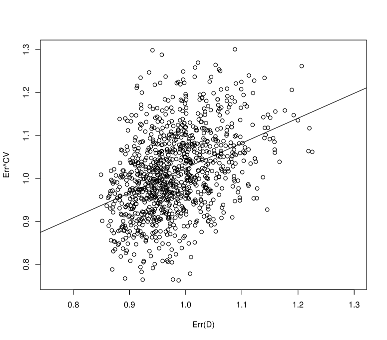
Figure 2: $Err(D)$ vs $\widehat{Err}_{m}^{CV}$ in estimating the mean absolute prediction error of a high dimensional linear regression

The lasso regularized estimator of the regression coefficient clearly does not follow a Gaussian distribution, and the theoretical justification for the Gaussian approximation of the cross-validated estimates provided for low dimensional setting is not applicable here. However, the empirical distribution of $\widehat{Err}^{CV}_{m}$ was quite “Gaussian” with its variance being approximated reasonably well by the proposed bootstrap method. This phenomena can be visualized by the QQ plot of $\widehat{Err}_{m}^{CV}$ with the smallest sample size of the training set, $m=40,$ in Figure 3, where the role of lasso regularization was expected to be the biggest. It is clear that the Gaussian approximation holds well empirically for both low and high dimensional settings. One possible explanation was that the mean absolute prediction error is a smooth function of the testing data, and thus the cross-validation estimator $\widehat{Err}^{CV}_{m}$ is still a regular root $n$ estimator of $Err_{m}$. This observation suggests a broader application of the proposed method for constructing confidence intervals for $Err_{m}.$

In summary, the proposed confidence interval has a reasonable coverage level but slightly conservative. Empirically, the interval can be viewed as confidence interval for both $Err(D_{n})$ and $Err_{m}$ when $m\approx n,$ although the procedure was designed for the latter. In this case, the confidence interval based on nested cross-validation also had a proper coverage level for both $Err(D_{n})$ and $Err_{m}$, even though the procedure was designed for the former. Furthermore, the bootstrap calibration can be used to maintain proper coverage level of confidence intervals constructed with a very small number of bootstraps at the cost of enlarging the resulting intervals.

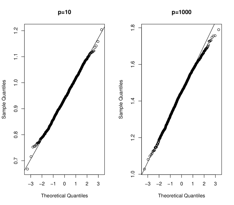
Figure 3: The QQ plot for the empirical distribution of $\widehat{Err}^{CV}_{m}$ for estimating the mean absolute prediction error

$m$	$p=10$						$p=1000$
	$Err_{m}$	$E(\widehat{Err}_{m}^{CV})$	SD	Cov-adj	Cov		$Err_{m}$	$E(\hat{Err}_{m}^{CV})$	SD	Cov-adj	Cov
40	0.941	0.938	0.077	96.7%	98.0%		1.441	1.445	0.123	97.3%	98.9%
45	0.920	0.918	0.076	96.9%	98.1%		1.334	1.341	0.126	97.0%	98.9%
50	0.906	0.904	0.075	96.5%	98.2%		1.248	1.255	0.121	97.4%	99.2%
55	0.894	0.892	0.074	96.4%	98.1%		1.179	1.187	0.115	97.6%	99.4%
60	0.885	0.883	0.074	96.0%	98.1%		1.128	1.134	0.109	98.2%	99.4%
65	0.877	0.875	0.074	95.5%	98.2%		1.087	1.093	0.103	98.6%	99.3%
70	0.870	0.869	0.073	94.9%	98.0%		1.058	1.060	0.100	98.4%	99.4%
75	0.865	0.864	0.073	94.6%	97.9%		1.031	1.034	0.097	98.5%	99.5%
80	0.861	0.859	0.073	93.3%	97.7%		1.012	1.013	0.097	97.9%	99.4%

Table 1: Simulation Results for estimating the mean absolute prediction error. $Err_{m}$, the true mean absolute prediction error; $E(\widehat{Err}_{m}^{CV}),$ the empirical average of the cross-validation estimate $\widehat{Err}_{m}^{CV}$; SD, the empirical standard deviation of the cross-validation estimate $\widehat{Err}_{m}^{CV}$ ; COV-adj, the empirical coverage level of 95% confidence intervals based on $\hat{\sigma}_{m,adj}^{CV}$ from bootstrap; COV, the empirical coverage level of 95% confidence intervals based on $\hat{\sigma}_{m}^{CV}$ from bootstrap.

$m$	Confidence Intervals Based on $\widehat{\sigma}_{m,adj}^{CV}$				Confidence Intervals based on $\widehat{\sigma}_{m}^{CV}$
	Algorithm 2	Algorithm 2	Algorithm 3		Algorithm 2	Algorithm 2	Algorithm 3
	$B_{BOOT}=400$	$B_{BOOT}=20$	$B_{BOOT}=20$		$B_{BOOT}=400$	$B_{BOOT}=20$	$B_{BOOT}=20$
	$p=10$
40	96.7%	95.1%	96.8%		98.0%	97.2%	98.4%
45	96.9%	95.2%	96.9%		98.1%	97.4%	98.7%
50	96.5%	94.6%	96.8%		98.2%	97.1%	98.8%
55	96.4%	94.4%	96.7%		98.1%	97.2%	98.9%
60	96.0%	93.2%	96.9%		98.1%	96.9%	98.7%
65	95.5%	93.1%	96.7%		98.2%	96.7%	98.9%
70	94.9%	93.1%	97.3%		98.0%	96.7%	99.1%
75	94.6%	91.6%	97.7%		97.9%	95.9%	98.8%
80	93.3%	89.8%	98.4%		97.7%	93.4%	99.1%
	$p=1000$
40	97.3%	95.9%	98.6%		98.9%	97.5%	99.3%
45	97.0%	95.3%	98.4%		98.9%	97.4%	99.3%
50	97.4%	95.6%	98.5%		99.2%	98.0%	99.4%
55	97.6%	96.4%	98.9%		99.4%	98.6%	99.7%
60	98.2%	97.2%	99.2%		99.4%	98.6%	99.7%
65	98.6%	97.3%	99.4%		99.3%	98.5%	99.9%
70	98.4%	97.5%	99.5%		99.4%	98.7%	99.8%
75	98.5%	96.5%	99.4%		99.5%	98.6%	99.8%
80	97.9%	96.1%	99.4%		99.4%	98.4%	99.7%

Table 2: Empirical coverage levels of 95% confidence intervals of the mean absolute prediction error using different numbers of bootstrap iterations.

3.1.3 Real Data Examples

The example is from the UCI machine learning repository. The dataset contains per capita violent crime rate and 99 prediction features for their plausible connection to crime in 1,994 communities after dropping communities and features with missing data. The crimes rate was calculated as the number of violated crimes per 100,000 residents in the community of interest. The violent crimes included murder, rape, robbery, and assault. The crime rate ranged from 0 to 1.0 with a median of 0.15. The predictors in the analysis mainly involved the community of interest, such as the percent of the urban population, the median family income, and law enforcement, such as per capita number of police officers, and percent of officers assigned to drug units. The objective of the analysis was to use these 99 community features to predict the violent crime rate. For demonstration purpose, we considered a subset consisting of first 600 observations as the observed dataset. First, we constructed the prediction model by fitting a linear regression model with lasso regularization, where the penalty parameter $\lambda$ was fixed at 0.005 for convenience. We applied our method for $m\in\{60,120,180,240,300,360,420,480,540\},$ i.e., the proportion of the observations used for training varied from 10%, to 20%, 30%, $\cdots$, 90%. Based on 500 cross-validations, the cross-validation estimate of the mean absolute prediction error for different training sizes was 0.141, 0.121, 0.115, 0.113, 0.111, 0.110, 0.109, 0.109 and 0.108, respectively. The 95% confidence interval for $Err_{m}^{CV}$ was then constructed based on the proposed bootstrap method. The number of bootstraps was 500 and the number of cross validations per bootstrap was 20. The results are summarized in Table 3. We also constructed the confidence interval for $Err(D_{n})$ using nested cross-validation. The resulting 95% confidence interval was [0.100, 0.116], which was fairly close to the bootstrap-based confidence interval for $Err_{540}^{CV}$ where the training size $m$ was the closest to $n=600.$

$m$	MAPE1	95% CI		MAPE	95% CI		$\Delta$ MAPE	95% CI
	Lasso			Random Forest			Difference2 $(\times 10^{-2})$
60	0.141	[0.128, 0.154]		0.121	[0.110, 0.132]		2.13	[1.50, 2.76]
120	0.121	[0.109, 0.133]		0.116	[0.105, 0.126]		0.58	[0.08, 1.09]
180	0.115	[0.105, 0.126]		0.113	[0.103, 0.124]		0.15	[-0.34, 0.64]
240	0.113	[0.102, 0.123]		0.112	[0.101, 0.122]		0.01	[-0.46, 0.48]
300	0.111	[0.101, 0.121]		0.111	[0.101, 0.122]		-0.05	[-0.51, 0.40]
360	0.110	[0.100, 0.120]		0.110	[0.100, 0.121]		-0.06	[-0.52, 0.41]
420	0.109	[0.100, 0.119]		0.109	[0.099, 0.120]		-0.05	[-0.52, 0.41]
480	0.109	[0.100, 0.118]		0.109	[0.098, 0.119]		-0.03	[-0.50, 0.44]
540	0.108	[0.099, 0.117]		0.108	[0.098, 0.118]		0.00	[-0.48, 0.48]
${}^{1}:$ mean absolute prediction error (MAPE).
${}^{2}:$ the difference in MAPE between the lasso regularized linear model and random forest.

Table 3: Results of estimating the mean absolute prediction error (MAPE) in predicting the crime rate based on community crime rate data from UCI repository

We have also considered a different prediction model trained using random forest. The output the random forest algorithm was an ensemble of 200 regression trees constructed based on bootstrapped samples. Based on 500 cross-validations, the cross-validation estimator of the mean absolute prediction error for different training sizes was 0.121, 0.116, 0.113, 0.112, 0.111, 0.110, 0.109, 0.109, and 0.108, respectively, smaller than those from lasso regularized linear regression model in general. The 95% confidence intervals using the proposed bootstrap method were reported in Table 3. Furthermore, the confidence interval for $Err(D_{600})$ based on nested cross-validation was [0.100, 0.115], which was also fairly close to the bootstrap-based confidence interval for $Err_{540}^{CV}$ as expected.

It appears that when sample size of the training data is small, the random forest generates more accurate predictions than the lasso-regularized linear model. When the sample size $m$ of the training set is greater than 200, however, the differences in prediction performance become very small. To account for the uncertainty, we also used the proposed bootstrap method to construct the 95% confidence interval for the difference in mean absolute prediction error between lasso regularized linear model and random forest. Indeed, when $m=60,$ the 95% confidence interval for the difference in $Err_{m}^{CV}$ was [1.50, 2.76] suggesting a statistically significantly better prediction performance of the random forest. The superiority of random forest also holds for $m=120.$ The results for other $m$ were reported in Table 3 showing no statistically significant difference between two prediction models.

3.2 Application 2

3.2.1 Theoretical Properties

In the second application, we are interested in estimating the c-index from a logistic regression model via cross-validation. In this case, it is not difficult to verify the conditions C1-C5 under conventional assumptions. For example, under the condition that there is no $\beta$ such that the hyperplane $\beta^{\prime}z=a_{0}$ can perfectly separate observations with $Y_{i}=1$ from those with $Y_{i}=0$ and the matrix

$$A_{0}=E\left[\tilde{Z}^{\prime}\tilde{Z}\frac{\exp(\beta^{\prime}\tilde{Z})}{\left\{1+\exp(\beta^{\prime}\tilde{Z})\right\}^{2}}\right]$$

is positive definite for all $\beta$, the maximum likelihood estimator based on the logistic regression, $\hat{\beta},$ converges to a deterministic limit $\beta_{0}$ in probability as $n\rightarrow\infty$ and

$$\sqrt{n}(\hat{\beta}-\beta_{0})=\frac{1}{\sqrt{n}}\sum_{i=1}^{n}A_{0}^{-1}\left(Y_{i}-\frac{\exp(\beta_{0}^{\prime}\tilde{Z}_{i})}{1+\exp(\beta_{0}^{\prime}\tilde{Z}_{i})}\right)+o_{p}(1),$$

and thus $C_{1}$ is satisfied [27]. Second, the class of functions $\{I(\beta^{\prime}\tilde{z}<0)\mid\beta\in\Omega\}$ is Donsker, where $\Omega$ is a compact set in $R^{p+1}$. This fact suggests that the U-process

$$U(\beta)=\sqrt{n}\left[L\left(D,\beta\right)-P\left(\beta^{\prime}(\tilde{Z}_{1}-\tilde{Z}_{2})<0\mid Y_{1}=0,Y_{2}=1\right)\right]$$

is stochastically continuous, where

$$L\left(D,\beta\right)=\frac{1}{m_{0}m_{1}}\sum_{Y_{i}=0}\sum_{Y_{j}=1}I(\beta^{\prime}\tilde{Z}_{i}<\beta^{\prime}\tilde{Z}_{j}),$$

$m_{g}=\sum_{i=1}^{n}I(Y_{i}=g).$ As a consequence, condition C2 is satisfied as $n\rightarrow\infty$ and $0<P(Y=1)<1.$ It is clear that $P\left(\beta^{\prime}(\tilde{Z}_{1}-\tilde{Z}_{2})<0\mid Y_{1}=0,Y_{2}=1\right)$ is differentiable in $\beta$ in a small neighborhood of $\beta_{0},$ if $\beta_{0}^{\prime}\tilde{Z}$ has a differentiable density function, which suffices for condition C3. Next, the central limit theorem for U-statistics implies that

$$\sqrt{n}\left[L\left(D,\beta_{0}\right)-P\left(\beta_{0}^{\prime}(\tilde{Z}_{1}-\tilde{Z}_{2})<0\mid Y_{1}=0,Y_{2}=1\right)\right]$$

converges weakly to a mean zero Gaussian distribution as $n\rightarrow\infty,$ if $0<P(Y=1)<1.$ Lastly, $E\left\{P\left(\hat{\beta}^{\prime}(\tilde{Z}_{1}-\tilde{Z}_{2})<0\mid Y_{1}=0,Y_{2}=1\right)\right\}-P\left(\beta_{0}^{\prime}(\tilde{Z}_{1}-\tilde{Z}_{2})<0\mid Y_{1}=0,Y_{2}=1\right)=O(|E(\hat{\beta})-\beta_{0}|)=o_{p}(n^{-1/2})$ and C5 is satisfied. Therefore, we expect that $\left(\widehat{Err}_{m}^{CV}-Err_{m}\right)$ can be approximated by a mean zero Gaussian distribution whose variance can be consistently estimated by the proposed bootstrap method. Note that we don’t need to assume that the logistic regression model is indeed correct for the conditional probability $P(Y=1|Z).$

3.2.2 Simulation Study

In the numerical study, we considered two settings corresponding to low and high dimensional covariates vector $Z_{i}.$ In the first setting, $Z_{i}$ followed a 10 dimensional standard multivariate normal distribution and the binary outcome $Y_{i}$ followed a Bernoulli distribution

$$P(Y_{i}=1|Z_{i})=\frac{\exp(\beta_{0}^{\prime}\tilde{Z}_{i})}{1+\exp(\beta_{0}^{\prime}\tilde{Z}_{i})},$$

where $\beta_{0}=(0,1.16,1.16,1.16,1.16,0,\cdots,0)^{\prime}.$ This regression coefficient was selected such that the mis-classification error of the optimal Bayesian classification rule was approximately 20%. We let the sample size $n=90$ and considered the cross-validation estimator $\widehat{Err}_{m}^{CV}$ for the c-index $Err_{m},m\in\{40,45,50,55,60,65,70,75,80\}.$ The true value of $Err_{m}$ was obtained by averaging c-indexes of 5,000 logistic regression models trained in different training sets of size $m$ in an independent testing set consisting of 200,000 observations. We also constructed the cross-validation estimator of $Err_{m}$ from 1,000 simulated datasets $D_{n}$ of size $n=90$ each. For each generated dataset, we divided the dataset into training and testing sets 400 times and calculated the resulting $\widehat{Err}_{m}^{CV}$ as the average of 400 c-indexes from testing sets. We first implemented the fast bootstrap method to estimate the variance of the cross-validated estimates with $B_{BOOT}=400$ bootstraps and $B_{CV}=20$ cross-validations per bootstrap. The 95% confidence interval for $Err_{m}$ was constructed accordingly. Based on results from 1,000 datasets, we summarized the empirical average and standard deviation of $\widehat{Err}_{m}^{CV}$ for c-index and the empirical coverage level of 95% confidence intervals based on bootstrap variance estimates. The results were reported in Table 4. We also examined the performance of the bootstrap calibration in algorithm 2 for constructing 95% confidence intervals with a very small number of bootstraps. To this end, we set $(B_{BOOT},B_{CV})=(20,50),$ and the corresponding results were summarized in Table 5. The cross-validation estimator $\widehat{Err}_{m}^{CV}$ was almost unbiased in estimating $Err_{m}$ with its empirical bias negligible in comparison with the standard deviation of $\widehat{Err}_{m}^{CV}.$ The empirical coverage level of 95% confidence intervals with $B_{BOOT}=400$ was fairly close to the nominal level. The coverage levels of the confidence intervals based on $\widehat{\sigma}_{m,adj}^{CV}$ were approximately 90%, lower than 95%, for $m=75,80.$ We also examined the empirical coverage level of confidence intervals based on $\widehat{\sigma}_{m,adj}^{CV}$ with respect to $Err(D_{n})$ for $m=80.$ The coverage level was 89.5%, similar to that for $Err_{m}.$ When a small number of bootstraps was used, the coverage level of the confidence interval was markedly lower than those constructed via a large number of bootstraps. However, with the proposed bootstrap calibration, the coverage level became comparable to those using $B_{BOOT}=400$ bootstraps. For example, when $m=80,$ the empirical coverage level of confidence intervals based on $\widehat{\sigma}_{m}^{CV}$ was 94.2% for $B_{BOOT}=400,$ 90.5% for $B_{BOOT}=20$ without calibration, but 98.2% for $B_{BOOT}=20$ after calibration. The median width the calibrated confidence intervals increased $11-40\%$ depending on $m$. In this particular setting, we have also examined the choice of $B_{CV}=25$ as in other simulation studies but observed a nontrivial proportion of zero variance component estimator for large $m$, suggesting insufficient number of bootstraps and cross-validation for differentiating intrinsic bootstrap variance from the Monte-Carlo variance due to cross-validation.

In the second set of numerical experiments, we have considered a high dimensional case where the dimension of $Z$, $p$ is set at 1000. To estimate $\beta_{0}$, we have employed the lasso-regularized logistic regression analysis, where $\hat{\beta}$ was the maximizer of

$$\frac{1}{n}\sum_{i=1}^{n}\left[(\alpha+\beta_{Z}^{\prime}Z_{i})Y_{i}-\log\left\{1+\exp(\alpha+\beta_{Z}^{\prime}Z_{i})\right\}\right]-\lambda_{0}|\beta_{Z}|_{1}.$$

To save computational time, the penalty parameter $\lambda_{0}$ was fixed at 0.10 in this simulation study. In this case, the lasso-regularized estimator $\hat{\beta}$ was not a root $n$ “regular” estimator and its distribution could not be approximated well by a Gaussian. Therefore, the regularity condition C1 was not satisfied. However, the estimation of the c-index in the testing set was a very “smooth” step based on U-statistic and therefore, we still expected that the cross-validation estimator of the c-index to approximately follow a Gaussian distribution, whose variance could be estimated well by the proposed bootstrap method. Letting the maximizer of the regularized objective function be denoted by $\hat{\alpha}$ and $\hat{\beta}_{Z}$, the c-index in the testing set is estimated by the concordance rate between $Y_{i}<Y_{j}$ and $\hat{\beta}_{Z}^{\prime}Z_{i}<\hat{\beta}_{Z}^{\prime}Z_{j}.$ For each of 1,000 simulated datasets, we computed $\widehat{Err}_{m}^{CV}$ for c-index, its variance estimator $\hat{\sigma}_{m}^{CV}$ via bootstrap, and the true prediction error $Err(D_{n}).$ We calculated and reported the true value of $Err_{m},$ empirical mean and standard deviation of $\widehat{Err}_{m}^{CV}$, and the empirical coverage level of 95% confidence intervals based on the proposed bootstrap variance estimator in Table 4. Similar to the low-dimensional case, Table 5 summarized the empirical coverage level of confidence intervals constructed only using a very small number of bootstraps. Similar to the low-dimensional case, the empirical bias of $\widehat{Err}_{m}^{CV}$ in estimating $Err_{m}$ was almost zero and the empirical coverage level of the 95% confidence interval was very close to the nominal level of 95%. There was a moderate over-coverage of confidence intervals based on bootstrap variance estimates $\widehat{\sigma}_{m}^{CV}.$ On the other hand, the empirical coverage level of those confidence intervals of $Err_{m},m=80$ with respect to $Err(D_{n})$ was 96.1%. The empirical correlation coefficient between $Err(D_{n})$ and $\widehat{\sigma}_{m}^{CV}$ was as high as 0.52 in this setting. When only a small number of bootstraps was used, the proposed bootstrap calibration recovered the coverage level to a comparable level of those using a large number of bootstraps. For example, when $m=70,$ the empirical coverage level of the confidence interval based on $\widehat{\sigma}_{m,adj}^{CV}$ was 93.9% for $B_{BOOT}=400,$ 91.9% for $B_{BOOT}=20$ before the bootstrap calibration, and 94.3% for the bootstrap $B_{BOOT}=20$ after calibration. The median width the calibrated confidence interval increased 10-14% depending on $m$.

In summary, the proposed confidence intervals have a reasonable coverage. The interval can be viewed as confidence interval for both $Err(D_{n})$ and $Err_{m}$ when $m\approx n,$ although the procedure was designed for the latter. In this case, the nested cross-validation is not directly applicable for c-index or ROC curve, since the parameter estimator in the test set doesn’t take a form of sum of independent, identically distributed random elements. Lastly, the bootstrap calibration can be used to effectively account for the variability of bootstrap variance estimator due to small number of bootstrap iterations in constructing confidence intervals for $Err_{m}.$

$m$	$p=10$						$p=1000$
	$Err_{m}$	$E(\widehat{Err}_{m}^{CV})$	SD	COV-adj	COV		$Err_{m}$	$E(\hat{Err}_{m}^{CV})$	SD	COV-adj	COV
40	0.799	0.800	0.041	94.7%	96.6%		0.573	0.570	0.049	97.3%	98.9%
45	0.810	0.812	0.041	94.6%	96.4%		0.588	0.585	0.059	96.2%	98.6%
50	0.820	0.822	0.042	94.3%	96.4%		0.607	0.602	0.067	94.3%	98.2%
55	0.827	0.829	0.042	93.8%	96.0%		0.623	0.618	0.075	92.7%	97.9%
60	0.833	0.835	0.043	93.3%	95.4%		0.641	0.635	0.083	92.4%	97.8%
65	0.838	0.839	0.043	92.9%	95.3%		0.659	0.652	0.089	91.7%	97.5%
70	0.842	0.843	0.043	92.0%	94.9%		0.674	0.669	0.092	93.8%	98.2%
75	0.845	0.847	0.043	91.0%	94.3%		0.691	0.685	0.098	93.9%	98.4%
80	0.847	0.849	0.043	89.5%	94.1%		0.706	0.702	0.105	94.8%	98.8%

Table 4: Simulation Results for estimating the AUC under the ROC curve in predicting binary outcomes, i.e., the c-index. $Err_{m}$, the true c-index value; $E(\widehat{Err}_{m}^{CV}),$ the empirical average of the cross-validation estimate $\widehat{Err}_{m}^{CV}$; SD, the empirical standard deviation of the cross-validation estimate $\widehat{Err}_{m}^{CV}$ ; COV-adj, the empirical coverage level of 95% confidence intervals based on $\hat{\sigma}_{m,adj}^{CV}$ from bootstrap; COV, the empirical coverage level of 95% confidence intervals based on $\hat{\sigma}_{m}^{CV}$ from bootstrap.

$m$	Confidence Intervals Based on $\widehat{\sigma}_{m,adj}^{CV}$				Confidence Intervals based on $\widehat{\sigma}_{m}^{CV}$
	Algorithm 2	Algorithm 2	Algorithm 3		Algorithm 2	Algorithm 2	Algorithm 3
	$B_{BOOT}=400$	$B_{BOOT}=20$	$B_{BOOT}=20$		$B_{BOOT}=400$	$B_{BOOT}=20$	$B_{BOOT}=20$
	$p=10$
40	94.7%	93.7%	95.4%		96.6%	95.5%	96.9%
45	94.6%	93.0%	94.9%		96.8%	95.1%	97.2%
50	94.3%	92.3%	94.9%		96.5%	95.2%	97.0%
55	94.2%	91.6%	94.3%		96.0%	95.0%	96.5%
60	93.4%	91.0%	94.0%		95.4%	94.3%	96.8%
65	93.1%	90.8%	94.5%		95.4%	94.2%	96.4%
70	92.1%	90.2%	94.7%		94.9%	93.4%	96.5%
75	91.1%	89.2%	95.7%		94.3%	93.0%	97.7%
80	89.3%	85.2%	97.5%		94.2%	90.5%	98.2%
	$p=1000$
40	97.3%	95.3%	98.7%		98.9%	97.4%	99.3%
45	96.2%	93.0%	97.3%		98.6%	96.2%	98.5%
50	94.3%	92.2%	95.4%		98.2%	95.7%	98.2%
55	92.7%	91.0%	94.9%		97.9%	95.2%	97.8%
60	92.4%	91.5%	94.5%		97.8%	95.0%	97.2%
65	91.7%	91.3%	93.9%		97.5%	94.9%	97.4%
70	93.8%	91.9%	94.2%		98.2%	95.6%	97.5%
75	93.9%	92.9%	94.6%		98.4%	96.3%	98.0%
80	94.8%	92.8%	96.7%		98.8%	96.0%	99.0%

Table 5: Empirical coverage levels of 95% confidence intervals of the AUC under the ROC curve (c-index) using various numbers of bootstrap iterations.

3.2.3 Real Data Examples

In the first example, we tested our proposed method on the MI dataset from UCI machine learning repository. The dataset contained 1700 patients and up to 111 predictors collected from the hospital admission up to 3 days after admission for each patient. We were interested in predicting all cause mortality. After removing features with more than 300 missing values, there were 100 prediction features available at the day 3 after admission including 91 features available at the admission. The observed data consisted of 652 patients with complete information on all 100 features. There were 72 binary, 21 ordinal, and 7 continuous features. Out of 652 patients, there were 62 deaths corresponding to a cumulative mortality of 9.5%. We considered training size $m\in\{196,261,326,391,456,522,587\},$ which represented 30% to 90% of the total sample size. We considered four prediction models, all trained by fitting a lasso regularized logistic regression. Model 1 was based on 91 features collected at the time of admission; Model 2 was based on 100 features collected up to day 3 after hospital admission; Model 3 was based on 126 features collected at the time of admission after converting all ordinal features into multiple binary features; and Model 4 was based on 159 features collected up to day 3 after converting all ordinal features into multiple binary features. For simplicity, we fixed the lasso penalty parameter at 0.01 for fitting Model 1 and Model 3, and 0.0075 for fitting Model 2 and Model 4.

First, we estimated the cross-validated c-index, which was the AUC under the ROC curve based on 500 random cross-validations. We then constructed the 95% confidence interval based on standard error estimated via the proposed bootstrap method. The number of the bootstraps and the number of cross validations per bootstrap were set at 400 and 20, respectively. The results were reported in Table 6. Model 1 and Model 2 had similar predictive performance with a small gain in c-index by including 8 additional features collected after hospital admission. Likewise, Model 3 and Model 4 had similar predictive performance, which, however, was inferior to that of Models 1 and 2, suggesting that converting ordinal predictive features into multiple binary features may had a negative impact on the prediction performance of the regression model. On the one hand, converting ordinal features into binary features allowed more flexible model fitting. On the other hand, this practice increased the number of features and ignored the intrinsic order across different levels of an ordinal variable. Therefore, it was not a surprise that Models 3 and 4 were not as accurate as Models 1 and 2. We then formally compared the model performance by constructing the 95% confidence interval for the difference in c-index between Model 1 and Model 2; between Model 1 and Model 3; and between Model 2 and Model 4. The detailed comparison results for all training sizes were reported in Table 7. It was interesting to note that all confidence intervals include zero, suggesting that none of the observed differences in c-index between different models are statistically significant at the 0.05 level.

In the second example for binary outcome, we tested our proposal on the “red wine” data set studied in [6]. The data set contained measurements for 1,599 red wine samples and was also available in the UCI Repository. Each of the wine samples was evaluated by wine experts for its quality, which was summarized on a scale from 0 to 10, with 0 and 10 representing the poorest and highest quality, respectively. 11 features including fixed acidity, volatile acidity, citric acid, residual sugar, chlorides, free sulfur dioxide, total sulfur dioxide, density, pH, sulphates and alcohol were also measured for all wine samples. [6] compared different data mining methods aiming to predict the ordinal quality score using these eleven features. Here, we conducted a simpler analysis to identify wine samples with a quality score above 6. To this end, we coded a binary outcome $Y=1$, if the quality was $\geq 7$ and 0, otherwise. We selected an observed data set consisting of first 400 wines samples from the “red wine” data set. Although the sample size was not small relative to the number of predictive features, there were only 40 observations with $Y=1$ in this subset. For the cross-validation, the training size $m\in\{200,240,280,320,360\}.$ We considered two prediction models: Model 1 was based on a regular logistic regression, and Model 2 was based on a random forest with 200 classification and regression trees. We estimated the c-index based on 500 random cross-validations for each training size $m$ based on the “observed” data set including $n=400$ wine samples. We then constructed 95% confidence interval for the c-index using the proposed bootstrap method with $(B_{BOOT},B_{CV})=(400,20).$ The results were reported in Table 8. It was clear that the random forest generated a substantially better prediction model than the logistic regression across all training sizes considered. The confidence intervals of the the difference in c-index were above zero when $m=320$ and 360, suggesting that the random forest was statistically significantly more accurate than the logistic regression model. It was also interesting to note that the performance of the random forest became better with increased training size, while the c-index of the logistic regression was relatively insensitive to $m.$ This was anticipated considering the fact that the random forest fitted a much more complex model than the simple logistic regression and could make a better use of information provided by more training data for improving the prediction accuracy at local regions of the covariate space.

We then used the cross-validation to estimate the entire ROC curve based on the random forest with 200 regression and classification trees. Due to the small number of cases in the data set, we used the pre-validation method described in Remark 1 of section 2.1.2, i.e., constructing the ROC curve based on risk score for all $n$ samples estimated via a 10-fold cross-validation. To remove the Monte-Carlo variability in randomly dividing data into 10 parts, the final ROC curve was obtained by averaging over ROC curves from 500 10-fold cross-validations. We also plotted the ROC curve without cross-validation, which was clearly overly optimistic, since the AUC of the ROC curve was 1, representing a prefect prediction! The same bootstrap method could be used to estimate the point-wise confidence intervals of the ROC curve. Specifically, 500 bootstrapped data sets were generated and ROC curves from 20 12-fold cross-validations per bootstrapped data set were calculated. 12-fold instead of 10-fold cross-validation was employed to adjust for the reduced effective sample size in the training set. The bootstrap variance estimators for sensitivities corresponding to specificity level at $5\%,10\%,\cdots,95\%$ were then obtained. The resulting confidence intervals representing the underlying predictive performance of the trained random forest were plotted in Figure 4, suggesting that the real sensitivity in external data would not reach 100% even for low specificity levels.

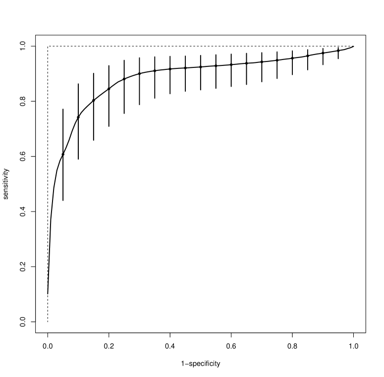
Figure 4: The naive ROC curve (dotted) and the ROC curve (solid) based pre-validation and 95% confidence intervals at selected specificity levels based on red wine data from UCI repository.

$m$	AUC	95% CI		AUC	95% CI
	91 features at Day 0			100 features at Day 3
196	0.711	[0.645, 0.778]		0.711	[0.643, 0.779]
261	0.729	[0.660, 0.798]		0.731	[0.659, 0.802]
326	0.743	[0.672, 0.814]		0.747	[0.674, 0.820]
391	0.753	[0.681, 0.825]		0.760	[0.687, 0.833]
456	0.759	[0.688, 0.831]		0.768	[0.695, 0.841]
522	0.766	[0.694, 0.837]		0.777	[0.705, 0.850]
587	0.771	[0.702, 0.840]		0.785	[0.718, 0.852]
	126 features at Day 0			159 features at Day 3
196	0.676	[0.596, 0.755]		0.664	[0.583, 0.745]
261	0.692	[0.610, 0.773]		0.678	[0.594, 0.762]
326	0.700	[0.616, 0.784]		0.688	[0.600, 0.776]
391	0.712	[0.628, 0.796]		0.702	[0.614, 0.791]
456	0.716	[0.631, 0.801]		0.709	[0.620, 0.798]
522	0.723	[0.640, 0.806]		0.718	[0.630, 0.805]
587	0.729	[0.644, 0.814]		0.727	[0.635, 0.819]

Table 6: Results of estimating the AUC under the ROC curve (c-index) based on MI data from UCI Repository.

$m$	$\Delta$ AUC	95% CI		$\Delta$ AUC	95% CI		$\Delta$ AUC	95% CI
	Models 2 vs. 1 $(\times 10^{-2})$			Models 1 vs. 3 $(\times 10^{-2})$			Models 2 vs. 4 $(\times 10^{-2})$
196	-0.042	[-2.361, 2.276]		3.562	[-1.400, 8.524]		4.714	[-0.647, 10.08]
261	0.189	[-2.469, 2.846]		3.729	[-1.571, 9.029]		5.268	[-0.564, 11.10]
326	0.387	[-2.432, 3.205]		4.317	[-1.300, 9.933]		5.900	[-0.293, 12.09]
391	0.711	[-2.076, 3.497]		4.158	[-1.468, 9.783]		5.795	[-0.621, 12.21]
456	0.878	[-1.963, 3.720]		4.341	[-1.560, 10.24]		5.906	[-0.690, 12.50]
522	1.157	[-1.810, 4.124]		4.307	[-1.699, 10.31]		5.976	[-0.731, 12.68]
587	1.370	[-1.508, 4.247]		4.222	[-1.998, 10.44]		5.804	[-1.338, 12.95]

Table 7: Results of comparing AUC under the ROC curve (c-index) between different prediction models based on MI data from UCI repository; Model 1: 91 features at Day 0; Model 2: 100 features at Day 3; Model 3: 126 features at Day 0; Model 4: 159 features at Day 3

$m$	AUC	95% CI		AUC	95% CI		$\Delta$ AUC	95% CI
	Logistic Regression			Random Forest			Difference
200	0.803	[0.737, 0.869]		0.855	[0.780, 0.929]		-0.052	[-0.112, 0.009]
240	0.811	[0.747, 0.875]		0.866	[0.791, 0.940]		-0.055	[-0.114, 0.004]
280	0.817	[0.753, 0.880]		0.874	[0.797, 0.951]		-0.057	[-0.118, 0.004]
320	0.823	[0.760, 0.881]		0.885	[0.812, 0.957]		-0.062	[-0.119, -0.005]
360	0.825	[0.770, 0.879]		0.897	[0.837, 0.958]		-0.073	[-0.129, -0.016]

Table 8: Results of estimating and comparing AUC under the ROC curve (c-index) based on red wine data from UCI Repository

3.3 Application 3

3.3.1 Theoretical Properties

In the third application, we are interested in evaluating the performance of a precision medicine strategy. In this case, it is not difficult to verify conditions C1-C5 under suitable assumptions. For example, if the matrix $A_{0}=E(\tilde{Z}\tilde{Z}^{\prime})$ is nonsingular, $P(G=1)=\pi\in(0,1)$, and $G\perp Z$, i.e., the treatment assignment is randomized, then $\hat{\gamma}$ and $\hat{\beta}$ converge to deterministic limits $\gamma_{0}$ and $\beta_{0},$ respectively, as $n\rightarrow\infty$, and especially

$$\sqrt{n}(\hat{\beta}-\beta_{0})=\frac{1}{\sqrt{n}}\sum_{i=1}^{n}\left\{\pi(1-\pi)A_{0}\right\}^{-1}\left\{Y_{i}-\gamma_{0}^{\prime}\tilde{Z}_{i}-(G_{i}-\pi)\beta_{0}^{\prime}\tilde{Z}_{i}\right\}+o_{p}(1),$$

where $\beta_{0}$ is an unique minimizer of the loss function

$$m(\beta)=E\left\{\left(Y^{(1)}-Y^{(0)}-\beta^{\prime}\tilde{Z}\right)^{2}\right\}.$$

Thus condition C1 is satisfied. Second, the classes of functions $\{yI(\beta^{\prime}z>0)\mid\beta\in\Omega\}$ , $\{yI(\beta^{\prime}z\leq 0)\mid\beta\in\Omega\}$, $\{I(\beta^{\prime}z>0)\mid\beta\in\Omega\}$, and $\{I(\beta^{\prime}z\leq 0)\mid\beta\in\Omega\}$ are Donsker, where $\Omega$ is a compact set in $R^{p+1}$. This fact suggests that the stochastic processes

$$\frac{1}{\sqrt{n}}\sum_{i=1}\left[Y_{i}I(\beta^{\prime}\tilde{Z}_{i}>0)-E\left\{YI(\beta^{\prime}\tilde{Z}>0)\right\}\right]$$

$$\frac{1}{\sqrt{n}}\sum_{i=1}\left[Y_{i}I(\beta^{\prime}\tilde{Z}_{i}\leq 0)-E\left\{YI(\beta^{\prime}\tilde{Z}\leq 0)\right\}\right]$$

$$\frac{1}{\sqrt{n}}\sum_{i=1}\left[I(\beta^{\prime}\tilde{Z}_{i}>0)-P(\beta^{\prime}\tilde{Z}>0)\right]$$

$$\frac{1}{\sqrt{n}}\sum_{i=1}\left[I(\beta^{\prime}\tilde{Z}_{i}\leq 0)-P(\beta^{\prime}\tilde{Z}\leq 0)\right]$$

are all stochastically continuous in $\beta.$ Therefore, the processes

$$U_{1}(\beta)=\sqrt{n}\left\{\frac{\sum_{i=1}^{n}Y_{i}G_{i}I(\beta^{\prime}\tilde{Z}_{i}>0)}{\sum_{i=1}^{n}G_{i}I(\beta^{\prime}\tilde{Z}_{i}>0)}-\frac{\sum_{i=1}^{n}Y_{i}(1-G_{i})I(\tilde{\beta}^{\prime}Z_{i}>0)}{\sum_{i=1}^{n}(1-G_{i})I(\tilde{\beta}^{\prime}Z_{i}>0)}-E\left(Y^{(1)}-Y^{(0)}\mid\beta^{\prime}\tilde{Z}>0\right)\right\}$$

and

$$U_{0}(\beta)=\sqrt{n}\left\{\frac{\sum_{i=1}^{n}Y_{i}G_{i}I(\beta^{\prime}\tilde{Z}_{i}\leq 0)}{\sum_{i=1}^{n}G_{i}I(\beta^{\prime}\tilde{Z}_{i}\leq 0)}-\frac{\sum_{i=1}^{n}Y_{i}(1-G_{i})I(\beta^{\prime}\tilde{Z}_{i}\leq 0)}{\sum_{i=1}^{n}(1-G_{i})I(\beta^{\prime}\tilde{Z}_{i}\leq 0)}-E\left(Y^{(1)}-Y^{(0)}\mid\beta^{\prime}\tilde{Z}\leq 0\right)\right\}$$

are also stochastically continuous in $\beta$, i.e., $U_{g}(\beta_{1})-U_{g}(\beta_{2})=o_{p}(1)$ for $\|\beta_{2}-\beta_{1}\|=o(1),g\in\{0,1\}.$ As a consequence, condition C2 is satisfied. It is clear that $l_{1}(\beta)=E\left(Y^{(1)}-Y^{(0)}\mid\beta^{\prime}\tilde{Z}>0\right)$ and $l_{0}(\beta)=E\left(Y^{(1)}-Y^{(0)}\mid\beta^{\prime}\tilde{Z}\leq 0\right)$ are differentiable in $\beta$ in a small neighborhood of $\beta_{0},$ if the random variable $\beta_{0}^{\prime}\tilde{Z}$ has a continuously differentiable bounded density function and $E\left(Y^{(g)}\mid\beta_{0}^{\prime}\tilde{Z}=s\right)$ is smooth in $s$. This suffices for condition C3. Next, the central limit theorem and delta-method together imply that $U_{g}(\beta_{0})$ converges weakly to a mean zero Gaussian distribution as $n\rightarrow\infty,$ where $g\in\{0,1\}.$ Lastly, $|E\{P(Y^{(1)}-Y^{(0)}\mid\hat{\beta}^{\prime}\tilde{Z}>0)\}-P(Y^{(1)}-Y^{(0)}\mid\beta_{0}^{\prime}\tilde{Z}>0)|+|E\{P(Y^{(1)}-Y^{(0)}\mid\hat{\beta}^{\prime}\tilde{Z}\leq 0)\}-P(Y^{(1)}-Y^{(0)}\mid\beta_{0}^{\prime}\tilde{Z}\leq 0)|=o_{p}(|E(\hat{\beta})-\beta_{0}|)=o_{p}(n^{-1/2}),$ and C5 is satisfied. Therefore, the cross-validation estimator $\widehat{Err}^{CV}_{m}$ is a consistent estimator for $Err_{m}$ and follows asymptotically a Gaussian distribution, whose variance can be estimated by the proposed bootstrap method.

3.3.2 Simulation Study

In the simulation study, the covariate $Z_{i}$ was generated from a $p$ dimensional standard multivariate Gaussian distribution and the continuous outcome $Y_{i}^{(g)}$ was generated via two linear regression models:

$$Y_{i}^{(1)}=\beta_{1}^{\prime}\tilde{Z}_{i}+\epsilon_{i}^{(1)},$$

and

$$Y_{i}^{(0)}=\beta_{0}^{\prime}\tilde{Z}_{i}+\epsilon_{i}^{(0)},$$

where $\beta_{1}=(0,0.25,0.25,0.25,0.25,0,\cdots,0)^{\prime}$, $\beta_{0}=(0,0.25,-0.25,0.25,-0.25,0,\cdots,0)^{\prime}$ and $\epsilon_{i}^{(g)}\sim N(0,1),g\in\{0,1\}.$ The treatment assignment indicator $\{G_{1},\cdots,G_{n}\}$ was a random permutation of $\{1,\cdots,1,0,\cdots,0\}$ consisting of $n/2$ ones and $n/2$ zeros. The observed outcome $Y_{i}=Y_{i}^{(1)}G_{i}+Y_{i}^{(0)}(1-G_{i}),i=1,\cdots,n.$ The generated data $D_{n}=\left\{X_{i}=(Y_{i},G_{i},Z_{i}),i=1,\cdots,n\right\}.$

In the first set of simulations, we let $p=10$ and the sample size $n=90\times 2=180$. We considered the cross-validation estimator $\widehat{Err}_{m}^{CV}$ for $Err_{m},m\in\{80,90,100,110,120,130,140\}.$ Due to symmetry, we only considered the case where $Err_{m}$ was the average treatment effect among patients recommended to receive treatment $G=1,$ denoted as the high value subgroup consisting of responders to the treatment $G=1$. The true value of $Err_{m}$ was computed by averaging the treatment effect among identified responders based on the estimated ITR scores from 5,000 generated training sets of size $m$. The true treatment effect among responders was calculated with an independently generated testing set consisting of 200,000 patients. The true $Err_{m}$ is 0.37, 0.39, 0.40, 0.42, 0.43, and 0.44 for $m=$ 80, 90, 100, 110, 120, 130, and 140, respectively. The increasing trend in $Err_{m}$ reflected the improved quality of the estimated ITR score based on a bigger training set. Note that in this setting, the average treatment effect among responders based on true individualized treatment effects was 0.56.

We constructed the cross-validation estimates of the $Err_{m}$ from 1,000 datasets $D_{n}$ of size $n=90$ each. For each simulated data set $D_{n}$, we divided the data set into a training set of size $m$ and a testing set of size $n-m$. The ITR score $\widehat{\Delta}(z\mid D_{train})$ was estimated based on the training set and responders in the testing set was identified as patients whose $\widehat{\Delta}(z\mid D_{train})>0$. The average treatment effect estimator among responders in the testing set was simply the average difference in $Y$ between responders, who received the active treatment $G=1,$ and responders, who received the control treatment $G=0.$ This process was repeated 400 times and the resulting $\widehat{Err}_{m}^{CV}$ was the sample average of 400 average treatment effect estimators among identified responders in the testing set. In addition, we used the proposed bootstrap method to compute the standard error estimators $\hat{\sigma}_{m}^{CV}$ and $\hat{\sigma}_{m,adj}^{CV}.$ In computing them, we set the number of bootstraps $B_{BOOT}$ to be 400 and the number of cross-validations per bootstrap to be $B_{CV}=20.$ The 95% confidence interval for $Err_{m}$ was also constructed for each simulated data set $D_{n}.$ We also examined the performance of constructed confidence intervals using only a very small number of bootstrap iterations by choosing $(B_{BOOT},B_{CV})=(20,25).$

In the second set of simulations, we let $p=1000.$ In calculating the estimated regression coefficient $\hat{\beta}$ in the ITR score $\widehat{\Delta}(z\mid D_{train}),$ we implemented the lasso regularized method. Specifically, we estimated $\beta$ by minimizing a regularized loss function

$$\sum_{X_{i}\in D_{train}}\left[Y_{i}-\gamma_{0}-\gamma_{Z}^{\prime}Z_{i}-(G_{i}-\pi)\beta^{\prime}\tilde{Z}_{i}\right]^{2}+\lambda_{1}|\gamma_{Z}|_{1}+\lambda_{2}|\beta|_{1},$$

where $\lambda_{1}$ and $\lambda_{2}$ were appropriate penalty parameters. To save computational time, both penalty parameters were fixed at 0.10 in all simulations instead of being adaptively selected via cross-validation within the training set. The resulting minimizer of $\beta$ was denoted by $\hat{\beta}(D_{train})$ and $\widehat{\Delta}(z\mid D_{train})=\hat{\beta}(D_{train})^{\prime}\tilde{z}.$ Similar to the low dimensional case, we simulated 1,000 datasets and for each generated dataset $D_{n},$ we calculated $Err(D_{n}),$ $\widehat{Err}_{m}^{CV}$, the bootstrap standard error estimators $\widehat{\sigma}_{m}^{CV}$ and $\widehat{\sigma}_{m,adj}^{CV}$, and the corresponding 95% confidence intervals. Similar to the low dimensional case, we investigated the performance of the confidence intervals constructed using both a large number and a small number of bootstraps.

The simulation results including the true value of $Err_{m}$, the empirical average and standard deviation of cross-validation estimator $\widehat{Err}_{m}^{CV}$, and the empirical coverage of 95% confidence intervals based on $B_{BOOT}=400$ were summarized in Table 9. In addition, the empirical coverage levels of the constructed 95% confidence intervals based on $B_{BOOT}=20$ were summarized in Table 10. For both low and high dimensional cases, the cross-validated estimator $\widehat{Err}^{CV}_{m}$ was almost unbiased in estimating $Err_{m}$, especially relative to the empirical standard deviation of $\widehat{Err}^{CV}_{m}$. The empirical coverage level of 1000 constructed 95% confidence intervals for $Err_{m}$ based on bootstrap variance estimator from a large number of bootstrap iterations was quite close to its nominal level. After sample size adjustment in variance estimation, the constructed confidence intervals based on $\widehat{\sigma}_{m,adj}^{CV}$ slightly under-covered the true parameter with empirical coverage levels between 90% and 93%. When a small number of bootstrap iterations was used ($B_{BOOT}=20$), the proposed bootstrap calibration can be used to maintain the proper coverage level as Table 10 showed. As a price, the median width of calibrated confidence interval increased 14-28% depending on the training size $m$ and dimension $p$. Note that the theoretical justification for the Gaussian approximation to the cross-validated estimator in high dimensional case was not provided as in the previous two examples. However, the empirical distribution of $\widehat{Err}^{CV}_{m}$ was quite “Gaussian” with its variance being approximated well by bootstrap method. This observation ensured the good performance of resulting 95% confidence intervals. In addition, the empirical coverage levels of the 95% confidence intervals of $Err_{m}$ with respect to $Err(D_{n})$ were 92.9% and 95.4% in low- and high- dimensional settings, respectively, where $(m,n)=(140,180).$

In summary, proposed confidence intervals based on bootstrap standard error estimator $\widehat{\sigma}_{m}^{CV}$ have a good coverage level. The bootstrap calibration can effectively correct the under-coverage of the confidence intervals based on a very small number of bootstraps. The constructed confidence interval can be viewed as a confidence interval for both $Err(D_{n})$ and $Err_{m},$ when $m\approx n$. In this case, due to the complexity of the evaluation procedure in the testing set, no existing method is readily available for studying the distribution of the cross-validation estimator for the average treatment effect among “responders”.

$m$	$p=10$						$p=1000$
	$Err_{m}$	$E(\widehat{Err}_{m}^{CV})$	SD	COV-adj	COV		$Err_{m}$	$E(\hat{Err}_{m}^{CV})$	SD	COV-adj	COV
80	0.369	0.377	0.196	92.7%	95.1%		0.079	0.082	0.190	92.7%	95.9%
90	0.384	0.395	0.197	91.9%	95.2%		0.094	0.095	0.198	92.0%	96.1%
100	0.398	0.409	0.198	92.3%	95.1%		0.108	0.110	0.208	91.1%	95.9%
110	0.412	0.422	0.199	91.9%	95.3%		0.119	0.123	0.218	91.3%	95.6%
120	0.421	0.433	0.199	91.4%	95.1%		0.135	0.138	0.229	91.0%	95.1&
130	0.431	0.441	0.201	90.7%	95.2%		0.152	0.152	0.242	90.3%	95.0%
140	0.439	0.449	0.202	91.4%	95.4%		0.166	0.166	0.256	89.4%	94.9%

Table 9: Simulation sesults for precision medicine. $Err_{m}$, the true average treatment effect in identified high value subgroup; $E(\widehat{Err}_{m}^{CV}),$ the empirical average of the cross-validation estimate $\widehat{Err}_{m}^{CV}$; SD, the empirical standard deviation of the cross-validation estimate $\widehat{Err}_{m}^{CV}$ ; COV-adj, the empirical coverage level of 95% confidence intervals based on $\hat{\sigma}_{m,adj}^{CV}$ from bootstrap; COV, the empirical coverage level of 95% confidence intervals based on $\hat{\sigma}_{m}^{CV}$ from bootstrap.

$m$	Confidence Intervals Based on $\widehat{\sigma}_{m,adj}^{CV}$				Confidence Intervals based on $\widehat{\sigma}_{m}^{CV}$
	Algorithm 1	Algorithm 1	Algorithm 2		Algorithm 1	Algorithm 1	Algorithm 2
	$B_{BOOT}=400$	$B_{BOOT}=20$	$B_{BOOT}=20$		$B_{BOOT}=400$	$B_{BOOT}=20$	$B_{BOOT}=20$
	$p=10$
80	92.7%	90.8%	94.8%		95.1%	93.7%	96.6%
90	91.9%	90.2%	94.1%		95.2%	92.7%	96.8%
100	92.3%	90.3%	94.6%		95.1%	93.0%	97.4%
110	91.9%	89.8%	95.3%		95.3%	93.5%	97.6%
120	91.4%	89.0%	96.7%		95.1%	93.3%	98.6%
130	90.7%	89.2%	96.5%		95.2%	92.4%	98.7%
140	91.4%	86.2%	97.1%		95.4%	90.9%	98.3%
	$p=1000$
80	92.7%	89.9%	94.2%		95.9%	93.1%	96.7%
90	92.0%	90.7%	95.4%		96.1%	93.9%	97.4%
100	91.1%	89.6%	95.8%		95.9%	93.9%	97.9%
110	91.3%	89.0%	95.0%		95.6%	93.7%	97.3%
120	91.0%	89.0%	94.5%		95.1%	93.8%	97.9%
130	90.3%	87.5%	95.0%		95.0%	93.6%	97.7%
140	89.4%	86.5%	96.0%		94.9%	92.6%	98.1%

Table 10: Empirical coverage levels of 95% confidence intervals of the average treatment effect among responders using various numbers of bootstrap iterations.

3.3.3 Real Data Example

In this section, we consider a recent clinical trial “Prevention of Events with Angiotensin Converting Enzyme Inhibition” (PEACE) to study whether the ACE inhibitors (ACEi) are effective in reducing future cardiovascular-related events for patients with stable coronary artery disease and normal or slightly reduced left ventricular function [14]. While a total of 8290 patients are enrolled in the study, we focus on a subgroup of 7865 patients with complete covariate information, in which 3947 and 3603 patients were assigned to receive the ACEi and placebo, respectively. One main endpoint of the study is the patient’s survival time. By the end of the study, there were 315 and 292 deaths observed in the control and treatment groups, respectively. Under a proportional hazards model, the estimated hazard ratio was 0.92 with a 95% confidence interval of (0.78, 1.08) and a two-sided p-value of 0.30. Based on the results of this study, it was inconclusive whether ACEi therapy would reduce the mortality in the overall patient population. However, with further analysis of the PEACE survival data, Solomon et al. (2006) reported that ACEi might significantly prolong the survival for patients whose baseline kidney functions were abnormal [24]. This finding could be quite important in guiding the individualized treatment recommendation in practice. The objective of our analysis here was systematic identification of a high value subgroup of patients who may benefited from ACEi, even though the average treatment effect of ACEi in the entire study population was neither clinically nor statistically significant. The outcome of interest was the time to all-cause mortality. To build a candidate ITR scoring system capturing the individualized treatment effect, we first used 4 covariates previously identified as statistically and clinically important predictors of the overall mortality in the literature [24]. These covariates are age, gender, eGFR measuring baseline renal function, and left ventricular ejection fraction measuring heart’s ability to pump oxygen-rich blood out to the body. We considered an ITR score derived from a training set of size $m=6292,$ i.e., 80% of the entire study population. The ITR score was the estimated difference in restricted mean survival time given baseline covariates [30, 35]. To this end, we fit Cox regression in two treatment arms separately:

$$P(Y_{i}>t|Z_{i}=z,G_{i}=g)=S_{g}(t)^{\exp(\beta_{g}^{\prime}z)}$$

and denote the resulting estimators by $\left\{\hat{S}_{g}(\cdot\mid D_{train}),\hat{\beta}_{g}(D_{train})\right\},$ where $S_{g}(t)$ is the baseline survival function and $\beta_{g}$ is the regression coefficient in treatment $g$ group, $g\in\{0,1\}.$ Specifically, $\beta_{g}$ can be estimated by maximizing the partial likelihood function and $S_{g}(\cdot)$ can be estimated by a transformation of the Breslow estimator of the cumulative baseline hazard function. Under the assumed Cox regression model, the ITR score for a patient with covariate $z$ is

$$\widehat{\Delta}(z\mid D_{train})=\int_{0}^{\tau}\left[\hat{S}_{1}(t\mid D_{train})^{\exp(\hat{\beta}_{1}(D_{train})^{\prime}z)}-\hat{S}_{0}(t\mid D_{train})^{\exp(\hat{\beta}_{0}(D_{train})^{\prime}z)}\right]dt,$$

where $\tau=2000$ days is a pre-specific cutoff time point. The average treatment effect in the testing set can be measured in different ways. First, we considered the average treatment effect as the difference in restricted mean survival time, representing by the area between the two survival curves restricted between time zero and the cutoff time point $\tau$, i.e.,

$$\hat{\Delta}_{g}(D_{train},D_{test})=\int_{0}^{\tau}\hat{S}_{1}(t\mid\hat{D}_{test}^{(g)})dt-\int_{0}^{\tau}\hat{S}_{0}(t\mid\hat{D}_{test}^{(g)})dt,$$

where $g\in\{0,1\},$

$$\hat{D}_{test}^{(1)}=\left\{X\in D_{test}\mid\hat{\Delta}(Z\mid D_{train})\geq\hat{\delta}_{0}\right\},$$

$$\hat{D}_{test}^{(0)}=\left\{X\in D_{test}\mid\hat{\Delta}(Z\mid D_{train})<\hat{\delta}_{0}\right\},$$

$\hat{\delta}_{0}$ was the sample median of $\left\{\widehat{\Delta}(Z\mid D_{train})\mid X\in D_{train}\right\},$ $\hat{S}_{1}(t\mid\hat{D}_{test}^{(g)})$ was the Kaplan-Meier estimator of the survival function based on patients in $\hat{D}_{test}^{(g)}$ who received the ACEi, and $\hat{S}_{0}(t\mid\hat{D}_{test}^{(g)})$ was the Kaplan-Meier estimator of the survival function based on patients in $\hat{D}_{test}^{(g)}$ who received the placebo. In other words, we were interested in estimating the average treatment effect in the high value subgroup and its complement. Furthermore, we are also interested in estimating the difference in average treatment effect between the high value subgroup and its complement, i.e., the interaction between treatment and subgrouping based on ITR scores. Here, the high value subgroup was identified by whether the estimated ITR score $\hat{\Delta}(z\mid D_{train})>\widehat{\delta}_{0}.$ Based on 500 cross-validations, the cross-validated estimate $\widehat{Err}^{CV}_{m}$ was 21.1 days for $\hat{\Delta}_{1}(D_{train},D_{test}),$ the average treatment effect in the high value subgroup, and -13.2 days for $\hat{\Delta}_{0}(D_{train},D_{test}),$ the average treatment effect in the complement of the high value subgroup. Their difference, i.e., the interaction with treatment, was 34.3 days. Now, we implemented the proposed bootstrap method to estimate the standard errors of those estimators. Specifically, we choose the number of bootstrap to be 500 and the number of cross-validation per bootstrap to be 20. The 95% confidence interval for the average treatment effect in the high value subgroup was [-1.3, 45.5] days, and the associated p value for testing no treatment effect was 0.064, nearly statistically significant at the conventional 0.05 level. The 95% confidence interval for the average treatment effect in the complement of the high value subgroup was [-31.5, 5.2] days and the associated p value for testing no treatment effect in that subgroup was 0.161. The 95% confidence interval for their difference was [4.3, 64.3] and the corresponding p value for testing no difference was 0.025, suggesting that the ITR score constructed from the training set of 6,292 patients had a statistically significant interaction with the treatment, i.e., the average treatment effect in the high value subgroup was greater than that in the remaining patients. The detailed results were summarized in Table 11.

Next, we also summarized the average treatment effect via the commonly used hazard ratio and the results were also reported in Table 11. The 95% confidence intervals of hazard ratios were transformed from confidence intervals of the log-transformed hazard ratio, whose distribution can be approximated better by a Gaussian distribution. Similarly, the comparison of two hazard ratios was based on the difference between two log-transformed hazard ratios or equivalently the ratio of two hazard ratios. Based on the hazard ratio, while the interaction between the identified high value subgroup and treatment was only marginally statistically significant at the 0.10 level, the average treatment effect in the high value subgroup was statistically significantly favoring ACEi. Lastly, we repeated the analysis with 7 baseline covariates: age, gender, eGFR, left ventricular ejection fraction, hypertension, diabetes, and history of myocardial infarction. The results were summarized in Table 11. The general directions of the result were similar as those based on 4 baseline covariates: the average treatment effect in the high value subgroup tended to be positive, while the average treatment effect in the complement of the high value subgroup tended to be negative after cross-validations. But no difference was statistically significant, which was expected because the three additional covariates didn’t demonstrate strong interactions with the treatment in previous analysis, and might dilute the predictiveness of the constructed ITR scores in capturing the individualized treatment effect [36].

restricted mean survival time					hazard ratio
$Err_{m}$	$\widehat{Err}_{m}^{CV}$	95% CI for $Err_{m}$	$p$ value		$Err_{m}$	$\widehat{Err}_{m}^{CV}$	95% CI for $Err_{m}$	$p$ value
4 covariates
$\hat{\Delta}_{1}$	21.1	[-1.3,43.5]	0.064		$\hat{\Delta}_{1}$	0.80	[0.66, 0.98]	0.028
$\hat{\Delta}_{0}$	-13.2	[-31.5, 5.2]	0.161		$\hat{\Delta}_{0}$	1.18	[0.85, 1.65]	0.326
$\hat{\Delta}_{1}-\hat{\Delta}_{0}$	34.3	[4.3, 64.3]	0.025		$\hat{\Delta}_{1}/\hat{\Delta}_{0}$	0.68	[0.44, 1.04]	0.076
7 covariates
$\hat{\Delta}_{1}$	17.9	[-3.9,39.7]	0.108		$\hat{\Delta}_{1}$	0.81	[0.66, 1.00]	0.053
$\hat{\Delta}_{0}$	-10.3	[-32.6, 12.1]	0.367		$\hat{\Delta}_{0}$	1.09	[0.79, 1.51]	0.603
$\hat{\Delta}_{1}-\hat{\Delta}_{0}$	28.1	[-5.4, 61.7]	0.100		$\hat{\Delta}_{1}/\hat{\Delta}_{0}$	0.75	[0.48, 1.15]	0.188

Table 11: Results of estimated the average treatment effect among identified responders in PEACE trial

There are other measures for the performance of a precision medicine strategy. For example, one may use the average utility (e.g., the RMST) when the strategy is applied to the entire patient population. One may also use the AD curve representing the average treatment effect in subgroups of patients with predicted treatment benefits above different cutoffs to gauge the performance of a strategy [36, 22]. They are not regular prediction errors, but should also be estimated via cross-validation to avoid overfitting. The bootstrap method proposed in this paper can be used to make rigorous statistical inference for them as well.

4 Discussion

In this paper, we propose a bootstrap method for making statistical inferences on summary statistics obtained from cross-validation, which is commonly used to evaluate the performance of statistical procedures. We clarify the population parameter that cross-validation estimates and provide asymptotic justification for the bootstrap procedure under certain regularity conditions. The proposed method substantially reduces the computational demands of a regular bootstrap using results from a random effects model and can be applied to quantify the uncertainty of almost any cross-validation-based estimate. Our approach complements the work of [2], which focuses on constructing confidence intervals for the random quantity $Err(D_{n})$.

However, there is a significant gap between the empirical performance of the proposed inference in finite samples and its theoretical justification, which requires large sample approximations and root $n$ regular estimates for all relevant parameters. For example, our simulation study shows that the distribution of the cross-validated estimate of the c-index of the logistic regression model with high-dimensional covariates fitted via lasso regularization is reasonably Gaussian, and the associated bootstrap confidence interval performs well even when the sample size is moderate. However, the current theoretical justification cannot confirm the validity of the proposed procedure in this setting, which is often the most important application of the cross-validation procedure. Therefore, further research in this direction is warranted.

We also note an interesting observation that although the bootstrap-based confidence intervals are constructed to cover the population parameter $Err_{m}$, they demonstrate a comparable coverage level with respect to $Err(D_{n})$ for $m\approx n.$ When the dimension is low, this can be explained by the fact that the variance of $Err(D_{n})$ is substantially smaller than that of $\widehat{Err}_{m}^{CV}$, and the correlation coefficient between $Err(D_{n})$ and $\widehat{Err}_{m}^{CV}$ is close to zero. When the dimension is high, however, the variance of $Err(D_{n})$ can be comparable to that of $\widehat{Err}_{m}^{CV}$, and the correlation between $Err(D_{n})$ and $\widehat{Err}_{m}^{CV}$ can be high. It is not clear when the constructed confidence interval can be interpreted as a confidence interval with respect to $Err(D_{n})$.

5 Appendix: Outline of the theoretical justification for the asymptotic normality of the cross-validation estimator $\widehat{Err}_{m}^{CV}$

First, based on condition $C1,$

$$\hat{\psi}(D_{train})-\psi_{0} =\frac{1}{m}\sum_{i\in D_{train}}\xi(X_{i})+o_{p}(m^{-1})$$ (3)

$$=\frac{1}{n}\sum_{i=1}^{n}\frac{I(X_{i}\in D_{train})}{\hat{\pi}}\xi(X_{i})+o_{p}(n^{-1}),$$ (4)

where $\hat{\pi}=m/n\in[l,u]$ and $0<l<u<1.$, Next, it follow from the condition $C2$ and $C3$ that

$$\sqrt{n-m}\left[L(D_{test},\hat{\psi}(D_{train}))-E\left\{L(D_{test},\hat{\psi}(D_{train}))\right\}\right]$$

$$= \sqrt{n-m}[L(D_{test},\psi_{0})-E\left\{L(D_{test},\psi_{0})\right\}]+o_{p}(1)$$

$$= \frac{1}{\sqrt{n-m}}\sum_{i\in D_{test}}\eta(X_{i})+o_{p}(1).$$

Note that

$$E\left\{L(D_{test},\hat{\psi}(D_{train})\right\}$$

$$= E\left\{L(D_{test},\psi_{0})\right\}+l_{\psi_{0}}(\hat{\psi}(D_{train})-\psi_{0})+o(\|\hat{\psi}(D_{train})-\psi_{0}\|)$$

$$= E\left\{L(D_{test},\psi_{0})\right\}+\frac{1}{n}\sum_{i=1}^{n}\frac{I(X_{i}\in D_{train})}{\hat{\pi}}l_{\psi_{0}}\left\{\xi(X_{i})\right\}+o_{p}(n^{-1})$$

based on condition C4 and (4). Lastly,

$$\sqrt{n}\left[E\left\{L(D_{test},\hat{\psi}(D_{train})\right\}-E\left\{L(D_{test},\psi_{0})\right\}\right]$$

$$= \sqrt{n}\left[E\left\{L(D_{test},\hat{\psi}(D_{train})\right\}-E\left\{L(D_{test},\hat{\psi}(D_{train}))\right\}\right]$$

$$+\sqrt{n}\left[E\left\{L(D_{test},\hat{\psi}(D_{train}))\right\}-E\left\{L(D_{test},\psi_{0})\right\}\right]$$

$$= \frac{\sqrt{n}}{(n-m)}\sum_{i\in D_{test}}\eta(X_{i})+\frac{1}{\sqrt{n}}\sum_{i=1}^{n}\frac{I(X_{i}\in D_{train})}{\hat{\pi}}l_{\psi_{0}}\left\{\xi(X_{i})\right\}+o_{p}(1)$$

$$= \frac{1}{\sqrt{n}}\sum_{i=1}^{n}\left[\frac{I(X_{i}\in D_{test})}{1-\hat{\pi}}\eta(X_{i})+\frac{I(X_{i}\in D_{train})}{\hat{\pi}}l_{\psi_{0}}\left\{\xi(X_{i})\right\}\right]+o_{p}(1).$$

Conditional on the observed data and taking expectation with respect to $I(X_{i}\in D_{train})$ and $I(X_{i}\in D_{test}),i=1,\cdots,n$

$$\sqrt{n}\left(\widehat{Err}^{CV}_{m}-E\left\{L(D_{test},\psi_{0})\right\}\right)=\frac{1}{\sqrt{n}}\sum_{i=1}^{n}\left[\eta(X_{i})+l_{\psi_{0}}\left\{\xi(X_{i})\right\}\right]+o_{p}(1).$$

Since $\lim_{n\rightarrow\infty}E\left\{L(D_{test},\psi_{0})\right\}=Err,$ we have

$$\sqrt{n}\left(\widehat{Err}^{CV}_{m}-Err\right)$$

converges weakly to a mean zero Gaussian distribution with a variance of

$$\sigma_{D}^{2}=E\left(\left[\eta(X_{i})+l_{\psi_{0}}\left\{\xi(X_{i})\right\}\right]^{2}\right).$$

Lastly, under condition C5,

$$\sqrt{n}\left(\widehat{Err}^{CV}_{m}-Err_{m}\right)=\sqrt{n}\left(\widehat{Err}^{CV}_{m}-Err\right)+o_{p}(1)$$

also converges weakly to $N(0,\sigma_{D}^{2}).$

References

• [1] Morgane Austern and Wenda Zhou. Asymptotics of cross-validation. arXiv preprint arXiv:2001.11111, 2020.
• [2] Stephen Bates, Trevor Hastie, and Robert Tibshirani. Cross-validation: what does it estimate and how well does it do it? arXiv preprint arXiv:2104.00673, 2021.
• [3] Pierre Bayle, Alexandre Bayle, Lucas Janson, and Lester Mackey. Cross-validation confidence intervals for test error. Advances in Neural Information Processing Systems, 33:16339โ€“16350, 2020.
• [4] Thomasย J Boardman. Confidence intervals for variance componentsโ€“a comparative monte carlo study. Biometrics, pages 251โ€“262, 1974.
• [5] Shuai Chen, Luย Tian, Tianxi Cai, and Menggang Yu. A general statistical framework for subgroup identification and comparative treatment scoring. Biometrics, 73(4):1199โ€“1209, 2017.
• [6] Paulo Cortez, Juliana Teixeira, Antรณnio Cerdeira, Fernando Almeida, Telmo Matos, and Josรฉ Reis. Using data mining for wine quality assessment. In Discovery Science: 12th International Conference, DS 2009, Porto, Portugal, October 3-5, 2009 12, pages 66โ€“79. Springer, 2009.
• [7] A.ย C. Davison and D.ย V. Hinkley. Bootstrap Methods and their Application. Cambridge Series in Statistical and Probabilistic Mathematics. Cambridge University Press, 1997.
• [8] Sandrine Dudoit and Markย J vanย der Laan. Asymptotics of cross-validated risk estimation in estimator selection and performance assessment. Statistical methodology, 2(2):131โ€“154, 2005.
• [9] Bradley Efron and Robert Tibshirani. Improvements on cross-validation: the 632+ bootstrap method. Journal of the American Statistical Association, 92(438):548โ€“560, 1997.
• [10] Bradley Efron and Robertย J Tibshirani. An introduction to the bootstrap. CRC press, 1994.
• [11] David Faraggi and Benjamin Reiser. Estimation of the area under the roc curve. Statistics in medicine, 21(20):3093โ€“3106, 2002.
• [12] Trevor Hastie, Robert Tibshirani, and Jerome Friedman. The elements of statistical learnin. Cited on, 33, 2009.
• [13] Brianย A Hemann, Williamย F Bimson, and Allenย J Taylor. The framingham risk score: an appraisal of its benefits and limitations. American Heart Hospital Journal, 5(2):91โ€“96, 2007.
• [14] PEACEย Trial Investigators. Angiotensin-convertingโ€“enzyme inhibition in stable coronary artery disease. New England Journal of Medicine, 351(20):2058โ€“2068, 2004.
• [15] Boย Jiang, Xuegong Zhang, and Tianxi Cai. Estimating the confidence interval for prediction errors of support vector machine classifiers. The Journal of Machine Learning Research, 9:521โ€“540, 2008.
• [16] Michaelย R Kosorok. Introduction to empirical processes and semiparametric inference. Springer, 2008.
• [17] Chayakrit Krittanawong, HongJu Zhang, Zhen Wang, Mehmet Aydar, and Takeshi Kitai. Artificial intelligence in precision cardiovascular medicine. Journal of the American College of Cardiology, 69(21):2657โ€“2664, 2017.
• [18] Nanย M Laird and Jamesย H Ware. Random-effects models for longitudinal data. Biometrics, pages 963โ€“974, 1982.
• [19] Erin LeDell, Maya Petersen, and Mark vanย der Laan. Computationally efficient confidence intervals for cross-validated area under the roc curve estimates. Electronic journal of statistics, 9(1):1583, 2015.
• [20] Jing Lei. Cross-validation with confidence. Journal of the American Statistical Association, 115(532):1978โ€“1997, 2020.
• [21] Pratik Patil, Yuting Wei, Alessandro Rinaldo, and Ryan Tibshirani. Uniform consistency of cross-validation estimators for high-dimensional ridge regression. In International Conference on Artificial Intelligence and Statistics, pages 3178โ€“3186. PMLR, 2021.
• [22] Fabio Pellegrini, Massimiliano Copetti, Francesca Bovis, David Cheng, Robert Hyde, Carl deย Moor, Berndย C Kieseier, and Mariaย Pia Sormani. A proof-of-concept application of a novel scoring approach for personalized medicine in multiple sclerosis. Multiple Sclerosis Journal, 26(9):1064โ€“1073, 2020.
• [23] Margaretย Sullivan Pepe. The statistical evaluation of medical tests for classification and prediction. Oxford University Press, USA, 2003.
• [24] Scottย D Solomon, Madelineย M Rice, Kathleen A.ย Jablonski, Powell Jose, Michael Domanski, Marc Sabatine, Bernardย J Gersh, Jean Rouleau, Marcย A Pfeffer, and Eugene Braunwald. Renal function and effectiveness of angiotensin-converting enzyme inhibitor therapy in patients with chronic stable coronary disease in the prevention of events with ace inhibition (peace) trial. Circulation, 114(1):26โ€“31, 2006.
• [25] Lisaย M Sullivan, Josephย M Massaro, and Ralphย B Dโ€™Agostinoย Sr. Presentation of multivariate data for clinical use: The framingham study risk score functions. Statistics in medicine, 23(10):1631โ€“1660, 2004.
• [26] Luย Tian, Ashย A Alizadeh, Andrewย J Gentles, and Robert Tibshirani. A simple method for estimating interactions between a treatment and a large number of covariates. Journal of the American Statistical Association, 109(508):1517โ€“1532, 2014.
• [27] Luย Tian, Tianxi Cai, Els Goetghebeur, and LJย Wei. Model evaluation based on the sampling distribution of estimated absolute prediction error. Biometrika, 94(2):297โ€“311, 2007.
• [28] Robert Tibshirani. Regression shrinkage and selection via the lasso. Journal of the Royal Statistical Society: Series B (Methodological), 58(1):267โ€“288, 1996.
• [29] Ryanย J Tibshirani and Robert Tibshirani. A bias correction for the minimum error rate in cross-validation. The Annals of Applied Statistics, 3(2):822โ€“829, 2009.
• [30] Hajime Uno, Brian Claggett, Luย Tian, Eisuke Inoue, Paul Gallo, Toshio Miyata, Deborah Schrag, Masahiro Takeuchi, Yoshiaki Uyama, Lihui Zhao, etย al. Moving beyond the hazard ratio in quantifying the between-group difference in survival analysis. Journal of clinical Oncology, 32(22):2380, 2014.
• [31] JSย Williams. A confidence interval for variance components. Biometrika, 49(1/2):278โ€“281, 1962.
• [32] Cortย J Willmott and Kenji Matsuura. Advantages of the mean absolute error (mae) over the root mean square error (rmse) in assessing average model performance. Climate research, 30(1):79โ€“82, 2005.
• [33] Steve Yadlowsky, Fabio Pellegrini, Federica Lionetto, Stefan Braune, and Luย Tian. Estimation and validation of ratio-based conditional average treatment effects using observational data. Journal of the American Statistical Association, 116(533):335โ€“352, 2021.
• [34] Waleedย A Yousef. Estimating the standard error of cross-validation-based estimators of classifier performance. Pattern Recognition Letters, 146:115โ€“125, 2021.
• [35] Lihui Zhao, Brian Claggett, Luย Tian, Hajime Uno, Marcย A Pfeffer, Scottย D Solomon, Lorenzo Trippa, and LJย Wei. On the restricted mean survival time curve in survival analysis. Biometrics, 72(1):215โ€“221, 2016.
• [36] Lihui Zhao, Luย Tian, Tianxi Cai, Brian Claggett, and Lee-Jen Wei. Effectively selecting a target population for a future comparative study. Journal of the American Statistical Association, 108(502):527โ€“539, 2013.