Murmurations of Dirichlet Characters

Abstract.

We calculate murmuration densities for two families of Dirichlet characters. The first family contains complex Dirichlet characters normalized by their Gauss sums. Integrating the first density over a geometric interval yields a murmuration function compatible with experimental observations. The second family contains real Dirichlet characters weighted by a smooth function with compact support. We show that the second density exhibits a universality property analogous to Zubrilina’s density for holomorphic newforms, and it interpolates the phase transition in the the $1$-level density for a symplectic family of $L$-functions.

1. Introduction

Following a programme of machine learning in arithmetic [HLO1, HLO2, HLO3], a striking oscillation in the average value of Frobenius traces for certain families of elliptic curves was observed in [HLOP]. This oscillation was termed a murmuration. In the original work, the average was taken over elliptic curves $E/\mathbb{Q}$ with conductor in certain intervals. Similar averages for other arithmetic families, including higher weight modular forms and higher genus curves, will be explored in [HLOPS].

After the initial observation, three important ideas emerged based on contributions of J. Ellenberg, A. Sutherland, J. Bober, and P. Sarnak. Firstly, on Ellenberg’s suggestion, Sutherland studied murmurations attached not only to newforms with rational coefficients, but, moreover, Galois orbits of those with coefficients in number fields. Secondly, Bober proposed a so-called local average, which eliminated the role played by the interval from the original construction. Thirdly, Sarnak introduced a notion of murmuration density, which involved additional averaging over primes and weighting by smooth functions of compact support [S23i]. To motivate his construction, Sarnak articulated the relationship between murmurations and the $1$-level densities for families of $L$-functions (see [S23ii]). All three ideas informed the important work of N. Zubrilina, in which a murmuration density for holomorphic newforms was calculated [Z23]. In this paper we calculate murmuration densities for two families of Dirichlet characters, both of which come from averaging characters over primes in short intervals (see Examples 2.3 and 2.4).

The first murmuration density we compute involves odd (resp. even) complex Dirichlet characters $\chi$ normalized by their Gauss sums $\tau(\chi)$. By way of justification, note that ${\chi}(p)/\tau(\chi)$ is the Fourier coefficient of $\overline{\chi}$ when expanded in terms of additive characters (see, e.g., [IK04, equation (3.12)]), and so this is a natural analogue of the modular form case. Integrating the murmuration density over a given geometric interval yields the average value of $\chi(p)/\tau(\chi)$ over odd (resp. even) Dirichlet characters with conductor in that interval, which is a scale invariant oscillation comparable with the murmuration first observed for elliptic curves (see Figure 5). More precisely, we let $\mathcal{D}_{+}(N)$ (resp. $\mathcal{D}_{-}(N)$) denote the set of primitive even (resp. odd) Dirichlet characters mod $N$. For $x\in\mathbb{R}_{>0}$, denote by $\lceil x\rceil^{\mathfrak{p}}$ the smallest prime that is bigger than or equal to $x$. For $c\in\mathbb{R}_{>1}$, $\delta\in(0,1)$, and $y\in\mathbb{R}_{>0}$, define

(1.1) $$P_{\pm}(y,X,c) =\frac{\log X}{X}\sum_{\begin{subarray}{c}N\in[X,cX]\\ N\text{ prime}\end{subarray}}\sum_{\chi\in\mathcal{D}_{\pm}(N)}\frac{\chi(\lceil yX\rceil^{\mathfrak{p}})}{\tau(\chi)},$$

(1.2) $$\widetilde{P}_{\pm}(y,X,\delta) =\frac{\log X}{X^{\delta}}\sum_{\begin{subarray}{c}N\in[X,X+X^{\delta}]\\ N\text{ prime}\end{subarray}}\sum_{\chi\in\mathcal{D}_{\pm}(N)}\frac{\chi(\lceil yX\rceil^{\mathfrak{p}})}{\tau(\chi)}.$$

We plot instances of the functions $P_{\pm}(y,X,c)$ and $\widetilde{P}_{\pm}(y,X,\delta)$ in Figure 1. The factors $\log(X)/X$ and $\log(X)/X^{\delta}$ are connected to the number of primes in the respective intervals. In the case of equation (1.2), we work conditional on the Riemann Hypothesis, which guarantees that the interval $[X,X+X^{\delta}]$ contains primes provided that $\delta>\frac{1}{2}$. Our first theorem is stated as follows:

Theorem 1.1.

Fix $y\in\mathbb{R}_{>0}$. If $c\in\mathbb{R}_{>1}$, then

(1.3) $$\lim_{X\to\infty}P_{\pm}(y,X,c)=\begin{cases}\int_{1}^{c}\cos\left(\frac{2\pi y}{x}\right)dx,&\text{ if }+,\\ -i\int_{1}^{c}\sin\left(\frac{2\pi y}{x}\right)dx,&\text{ if }-,\end{cases}$$

and, assuming the Riemann Hypothesis, if $\delta\in(\frac{1}{2},1)$, then

(1.4) $$\lim_{X\to\infty}\widetilde{P}_{\pm}(y,X,\delta)=\begin{cases}\cos(2\pi y),&\text{ if $+$},\\ -i\sin(2\pi y),&\text{ if $-$}.\end{cases}$$

The proof of Theorem 1.1 uses the prime number theorem, and the relationship between additive and multiplicative characters. Upon closer inspection, the proof of Theorem 1.1 indicates that equation (1.4) may be reformulated to incorporate certain composite conductors. We specify this reformulation in Section 6, and furthermore establish variants of Theorem 1.1 for arbitrary conductors (in which case we no longer need to assume the Riemann Hypothesis).

The second murmuration density we compute is the more challenging case of real Dirichlet characters. In this case, the average value of the Fourier coefficients for those with conductor in a geometric interval yields a noisy image (see Figure 4). To counteract this, we use techniques originally developed by Katz–Sarnak and refined by Soundararajan [S00]. For $d\in\mathbb{Z}$, we use the notation $\chi_{d}=\left(\frac{d}{\cdot}\right)$, and let $\mathcal{F}$ be the set of odd squarefree integers. If $d\in\mathcal{F}$ and $d>0$ (resp. $d<0$), then $\chi_{8d}$ is an even (resp. odd) primitive real character of conductor $8d$. For a smooth Schwartz function $\Phi\geq 0$ with compact support, define

(1.5) $$M_{\Phi}(y,X,\delta)=\frac{\log X}{X^{1+\delta}}\sum_{\begin{subarray}{c}p\in[yX,yX+X^{\delta}]\\ p\text{ prime}\end{subarray}}\sum_{\begin{subarray}{c}d\in\mathcal{F}\end{subarray}}\Phi\left(\frac{d}{X}\right)\chi_{8d}(p)\sqrt{p}.$$

Notice that one can isolate even (resp. odd) characters in this sum by choosing $\Phi$ to have compact support in $\mathbb{R}_{>0}$ (resp. $\mathbb{R}_{<0}$). For plots of these functions, see Figure 2.

Theorem 1.2.

Fix $y\in\mathbb{R}_{>0}$. If $\delta\in(\frac{1}{2},1)$ and $\Phi\geq 0$ is a smooth Schwartz function with compact support, then, assuming the Generalized Riemann Hypothesis, we have

(1.6) $$M_{\Phi}(y,\delta)\coloneqq\lim_{X\rightarrow\infty}M_{\Phi}(y,X,\delta)=\frac{1}{2}\sum_{\begin{subarray}{c}a=1\\ (a,2)=1\end{subarray}}^{\infty}\frac{\mu(a)}{a^{2}}\sum_{m=1}^{\infty}(-1)^{m}\widetilde{\Phi}\left(\frac{m^{2}}{2a^{2}y}\right),$$

where

(1.7) $$\widetilde{\Phi}(\xi)=\int_{-\infty}^{\infty}\left(\cos(2\pi\xi x)+\sin(2\pi\xi x)\right)\Phi(x)dx.$$

Although the smoothness of $\Phi$ is crucial in enabling the analytic tools used in the proof, we expect Theorem 1.2 to hold for weight functions with a sharp cut-off as well (we refer to Figure 3 for numerical support of this claim).

We remark that a density for a family of real Dirichlet characters was first computed by Rubinstein and Sarnak in [S23ii]. Their formula seems different from ours though the numerical values coincide approximately. Rubinstein and Sarnak also noted that the murmuration density interpolates the phase transition for the $1$-level density of a symplectic family, which emerges from our analysis in the following form.

Corollary 1.3.

Let $\Phi$ be a Schwartz function with compact support and let $\delta\in(\frac{1}{2},1)$. Assuming the Generalized Riemann Hypothesis, we have

(1.8) $$\lim_{y\rightarrow 0^{+}}M_{\Phi}(y,\delta)=0\quad\text{ and }\quad\lim_{y\rightarrow\infty}M_{\Phi}(y,\delta)=-\frac{2}{\pi^{2}}\widetilde{\Phi}(0),$$

where $M_{\Phi}(y,\delta)$ is defined in equation (1.6).

We present a proof of Corollary 1.3 in Section 5 that is less involved than the argument given by Rubinstein and Sarnak. On the other hand, Rubinstein and Sarnak evaluate the density as $y\to 0^{+}$ exactly, whereas we just bound it by a function that vanishes in the limit.

The proof of Theorem 1.2 involves identities for the Möbius function, the Polya–Vinogradov inequality for sums over primes, and Poisson summation as in [S00, Lemma 2.6]. The transform in equation (1.7) was used in [S00, Section 2.4]. Unfolding this transform and applying the identity $\cos(x)+\sin(x)=\sqrt{2}\cos(x-\pi/4)$ to equation (1.7) we conclude that

(1.9) $$\begin{split}\lim_{X\to\infty}M_{\Phi}(y,X,\delta)&=\frac{1}{2}\sum_{\begin{subarray}{c}a=1\\ (a,2)=1\end{subarray}}^{\infty}\frac{\mu(a)}{a^{2}}\sum_{m=1}^{\infty}(-1)^{m}\int_{-\infty}^{\infty}\left(\cos\left(\frac{\pi m^{2}x}{a^{2}y}\right)+\sin\left(\frac{\pi m^{2}x}{a^{2}y}\right)\right)\Phi(x)dx\\ &=\int_{-\infty}^{\infty}\Phi(x)\left(\frac{\sqrt{2}}{2}\sum_{\begin{subarray}{c}a=1\\ (a,2)=1\end{subarray}}^{\infty}\frac{\mu(a)}{a^{2}}\sum_{m=1}^{\infty}(-1)^{m}\cos\left(\frac{\pi m^{2}x}{a^{2}y}-\frac{\pi}{4}\right)\right)dx.\end{split}$$

In other words, conditional on the Generalized Riemann Hypothesis, we exhibit a distribution $M$ such that, for every smooth Schwartz $\Phi\geq 0$ with compact support and every $\delta\in(\frac{1}{2},1)$, we have

(1.10) $$\lim_{X\rightarrow\infty}M_{\Phi}(y,X,\delta)=\int_{-\infty}^{\infty}\Phi(t)M(y/t)dt.$$

Consequently, using Sarnak’s terminology, the distribution $M$ in equation (1.10) is the Zubrilina density for the family $\left\{\left(\frac{8d}{\cdot}\right):d\in\mathcal{F}\right\}$ [S23ii]. Using the same techniques, we calculate the Zubrilina density for $\left\{\left(\frac{d}{\cdot}\right):d\in\mathcal{F}\right\}$ in Section 6.2 and deduce the analogue of Corollary 1.3. Given Figure 3, it is not immediately clear whether or not $M$ exhibits infinitely many sign changes near $0$. Zubrilina has shown that, in the setting of modular forms, there are only finitely many sign changes.

We conclude this introduction with a summary of the sequel. Section 2 contains the relevant background material on Dirichlet characters. In Section 3, we prove Theorem 1.1. In Section 4, we prove Theorem 1.2. In Section 5, we prove Corollary 1.3. In Section 6, we state and prove the aforementioned variations on Theorems 1.1 and 1.2 (both of which concern averaging over an alternative set of conductors).

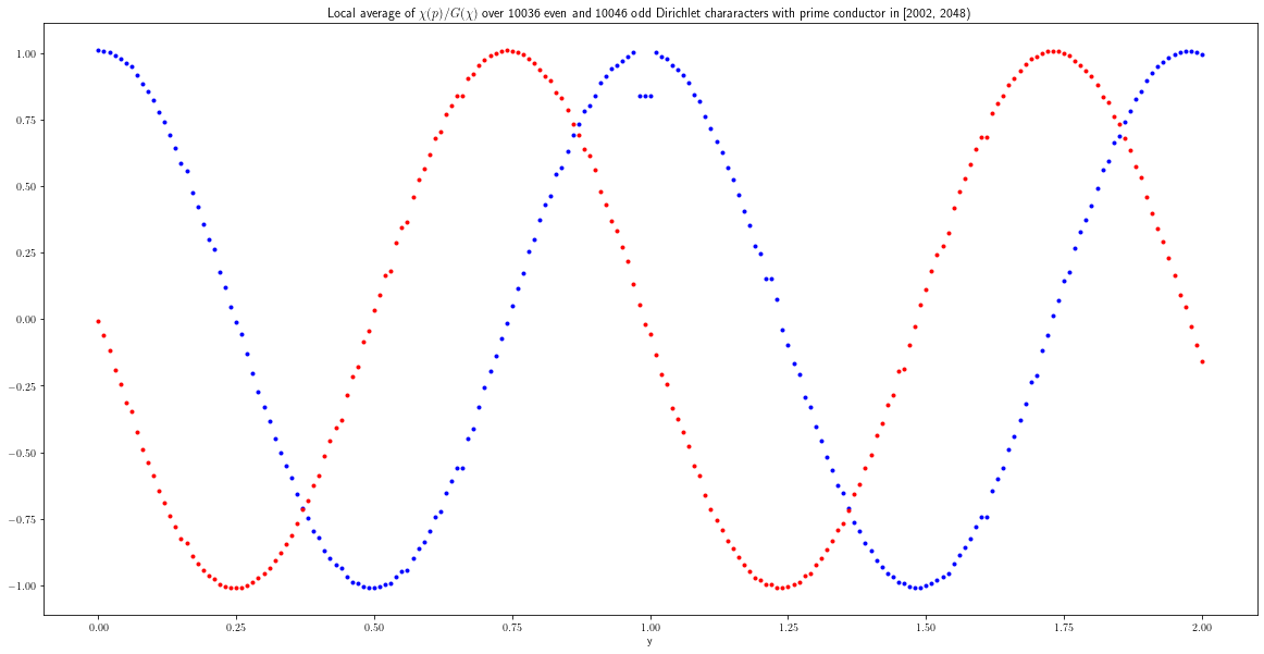
Figure 1. (Top) $P_{\pm}(y,2^{10},2)$ for $y\in[0,10]$ with $+$ in blue and (the imaginary part of) $-$ in red. (Bottom) $\widetilde{P}_{\pm}(y,2002,0.51)$ for $y\in[0,2]$ with $+$ in blue and (the imaginary part of) $-$ in red. The discontinuity around $y=1$ will be explained in Remark 3.1.

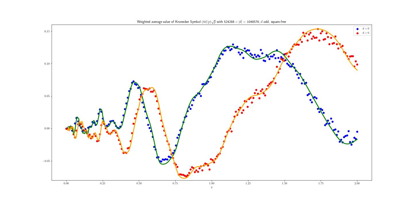
Figure 2. We plot $M_{\Phi_{\pm}}(y,2^{19},\frac{2}{3})$ for $y\in[0,2]$ with $+$ in blue (resp. $-$ in red), and the right hand side of equation (1.6) in green (resp. orange), where $\Phi_{+}(x)=\mathbbm{1}_{(1,2)}(x)\exp(\tfrac{-1}{1-4(x-1.5)^{2}})$ and $\Phi_{-}(x)=\mathbbm{1}_{(-2,-1)}(x)\exp(\tfrac{-1}{1-4(-x-1.5)^{2}})$.

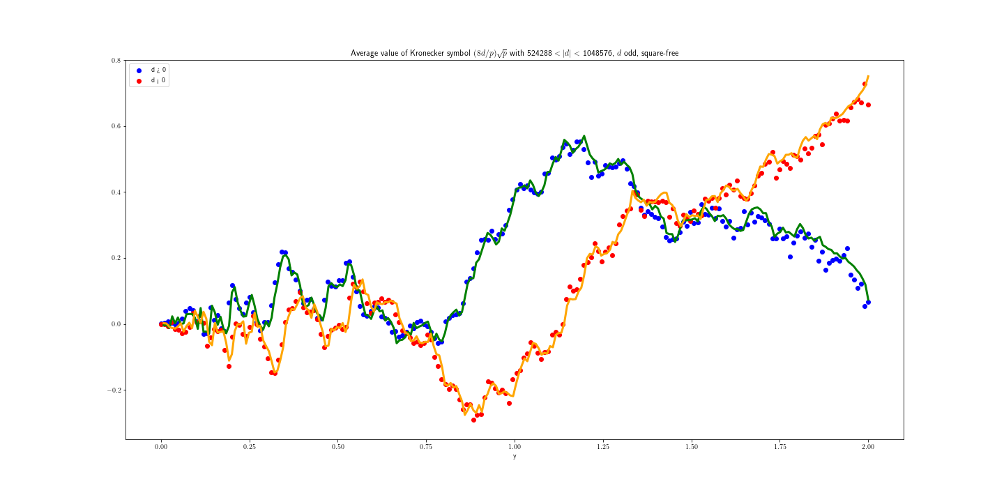
Figure 3. Let $\Phi_{+}(x)=\mathbbm{1}_{(1,2)}(x)$ and $\Phi_{-}(x)=\mathbbm{1}_{(-2,-1)}(x)$. We plot $M_{\Phi_{+}}(y,2^{19},\frac{2}{3})$ (resp. $M_{\Phi_{-}}(y,2^{19},\frac{2}{3})$) in blue (resp. red) and the right hand side of equation (1.6) in green (resp. orange).

Acknowledgements

The authors are grateful to Yang-Hui He and Andrew Sutherland for preliminary conversations connected to the themes of this paper, to Kumar Murty for helpful comments on an early draft, to Peter Sarnak for suggesting the use of Poisson summation and several insightful discussions, and to an anonymous referee for recommending that we include the family of real Dirichlet characters into this article.

2. Background

2.1. Asymptotics of double averages

For $m\in\mathbb{Z}_{>0}$, a Dirichlet character mod $m$ is a completely multiplicative function $\chi:\mathbb{Z}\rightarrow\mathbb{C}$ which is periodic with period $m$ and satisfies $\chi(a)=0$ if and only if $\mathrm{gcd}(a,m)>1$. The Gauss sum of a Dirichlet character $\chi$ mod $m$ is defined by

$$\tau(\chi)=\sum_{b=1}^{m}\chi(b)e^{2\pi ib/m}.$$

We denote by $\chi_{0}$ the principal Dirichlet character mod $m$, which satisfies $\chi_{0}(a)=1$ for $(a,m)=1$ by definition. We say that a Dirichlet character $\chi$ is even (resp. odd) if $\chi(-1)=1$ (resp. $\chi(-1)=-1$). The conductor of a Dirichlet character $\chi$ is the minimal positive integer $N$ such that $\chi$ is a Dirichlet character mod $N$. We say that a Dirichlet character $\chi$ is primitive if its modulus and conductor are equal. We let $\mathcal{D}_{+}(N)$ (resp. $\mathcal{D}_{-}(N)$) denote the set of primitive even (resp. odd) Dirichlet characters mod $N$. A Dirichlet character is said to be quadratic if its values are real. We denote by $\mathcal{Q}_{\pm}(N)$ the subset of $\mathcal{D}_{\pm}(N)$ consisting of quadratic characters. Note that, for even (resp. odd) characters $\chi\in\mathcal{Q}_{\pm}(N)$, we have $\tau(\chi)=\sqrt{N}$ (resp. $i\sqrt{N}$).

Example 2.1.

Quadratic characters provide the simplest analogue to the murmurations of elliptic curves over $\mathbb{Q}$ discovered in [HLOP]. Furthermore, using quadratic reciprocity, one may relate sums of quadratic Dirichlet characters to Chebyshev’s bias (cf. [RS94]). In Figure 4, we plot the sum of $\chi(p)/\tau(\chi)$ over $\bigcup_{N=X}^{2X-1}\mathcal{Q}_{\pm}(N)$ for $X=2^{17}$.

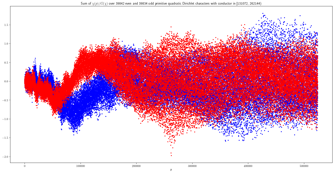
Figure 4. Plot of $\sum_{N\in[X,2X)}\sum_{\chi\in\mathcal{Q}_{\pm}(N)}\chi(p)/\tau(\chi)$, for $X=2^{17}$ and $2\leq p<4X$ with $+$ in blue and (the imaginary part of) $-$ in red.

In this paper, we follow two strategies for removing the noise from Figure 4. One strategy involves incorporating (Galois orbits of) complex characters into the average, and the other involves incorporating a smooth weight function with compact support. A theme common to both strategies is averaging over the primes.

Example 2.2.

In Figure 5, we plot the sum of $\chi(p)/\tau(\chi)$ over $\chi\in\bigcup_{N=X}^{2X-1}\mathcal{D}_{\pm}(N)$, for $X=2^{10}$, normalized by (cf. [J73]):

(2.1) $$\frac{1}{X}\sim\frac{3\sqrt{3}}{\pi^{2}\sqrt{\#\mathcal{D}_{\pm}(X)}}$$

We note that including the non-real characters and normalizing in this way removes the noise from Figure 4. We will observe a similar effect with modular forms in a forthcoming work [HLOPS].

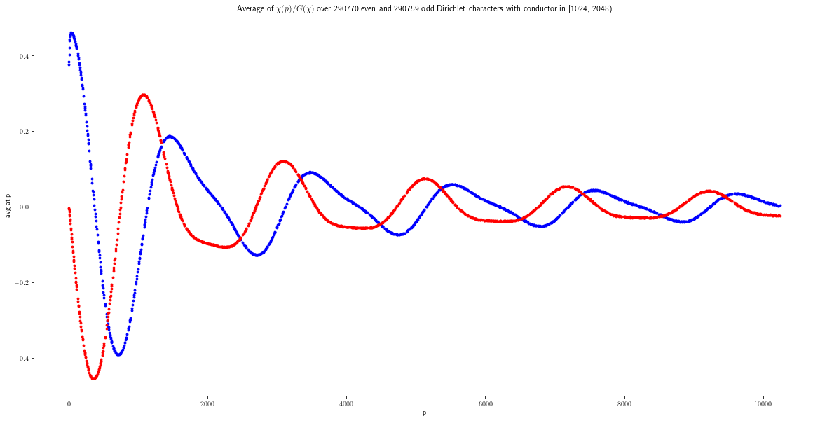
Figure 5. Plot of $\frac{1}{X}\sum_{N\in[X,2X)}\sum_{\chi\in\mathcal{D}_{\pm}(N)}\chi(p)/\tau(\chi)$ for $X=2^{10}$ for primes $p$ such that $2\leq p\leq 10X$, with $+$ in blue and (the imaginary part of) $-$ in red.

Example 2.3.

The function $\widetilde{P}_{\pm}(y,X,\delta)$ in equation (1.2) comes from the following average:

(2.2) $$\frac{\sum_{\begin{subarray}{c}N\in[X,X+X^{\delta}]\\ N\text{ prime}\end{subarray}}\sum_{\chi\in\mathcal{D}_{\pm}(N)}\chi(\lceil yX\rceil^{\mathfrak{p}})/\tau(\chi)}{\sum_{\begin{subarray}{c}N\in[X,X+X^{\delta}]\\ N\text{ prime}\end{subarray}}\,1},$$

where $y\in\mathbb{R}_{>0}$ and $\delta\in(\frac{1}{2},1)$. Indeed, using the prime number theorem, we deduce

(2.3) $$\lim_{X\rightarrow\infty}\left[\#\left\{N\in[X,X+X^{\delta}]:N~{}\text{prime}\right\}\cdot\frac{\log(X)}{X^{\delta}}\right]=1.$$

It follows that the function in equation (2.2) is asymptotic to $\widetilde{P}_{\pm}(y,X,\delta)$. There is a similar interpretation for the equation $P_{\pm}(y,X,c)$ in equation (1.1).

Example 2.4.

The function $M_{\Phi}(y,X,\delta)$ in equation (1.5) comes from the following double average:

(2.4) $$D_{\Phi}(y,X,\delta)=\frac{\sum_{\begin{subarray}{c}p\in[yX,yX+X^{\delta}]\\ p\text{ prime}\end{subarray}}\frac{\sum_{d\in\mathcal{F}}\Phi(d/X)\chi_{8d}(p)\sqrt{p}}{\sum_{d\in\mathcal{F}}\Phi(d/X)}}{\sum_{\begin{subarray}{c}p\in[yX,yX+X^{\delta}]\\ p\text{ prime}\end{subarray}}\,1},$$

where $y\in\mathbb{R}_{>0}$, $\delta\in(\frac{1}{2},1)$, $\Phi$ is a smooth function of compact support, $\mathcal{F}$ denotes the set of odd squarefree integers, and $\chi_{d}$ denotes the Kronecker symbol $\left(\frac{d}{\cdot}\right)$. Using the prime number theorem, we deduce

(2.5) $$\lim_{X\rightarrow\infty}\left[\#\left\{p\in[yX,yX+X^{\delta}]:p~{}\text{prime}\right\}\cdot\frac{\log(X)}{X^{\delta}}\right]=1.$$

It follows that $D_{\Phi}(y,X,\delta)$ is asymptotic to

(2.6) $$\frac{\log X}{X^{\delta}}\sum_{\begin{subarray}{c}p\in[yX,yX+X^{\delta}]\\ p\text{ prime}\end{subarray}}\frac{\sum_{d\in\mathcal{F}}\Phi(d/X)\chi_{8d}(p)\sqrt{p}}{\sum_{d\in\mathcal{F}}\Phi(d/X)}.$$

To simplify the denominator in equation (2.6), we note that the natural density of $\mathcal{F}$ is shown to be $4/\pi^{2}$ in [J10]. Using the fact that $\Phi$ is Schwartz, an equidistribution argument for $(d/X)_{d\in\mathcal{F}}$ implies that

(2.7) $$\lim_{X\to\infty}\frac{1}{X}\sum_{d\in\mathcal{F}}\Phi(d/X)=\frac{4}{\pi^{2}}~{}\int_{-\infty}^{\infty}\Phi(\tau)d\tau<\infty.$$

Therefore, to understand asymptotics of $D_{\Phi}(y,X,\delta)$, it suffices to analyse the limit of $M_{\Phi}(y,X,\delta)$.

2.2. Lemmas for Theorem 1.1

We begin with the following lemma on Gauss sums.

Lemma 2.5.

Let $N$ be a positive integer. If $p$ is a prime such that $(p,N)=1$, then

(2.8) $$\cos\left(\frac{2\pi p}{N}\right) =\frac{-1}{\phi(N)}+\frac{1}{\phi(N)}\sum_{\begin{subarray}{c}\chi\bmod N\\ \ \chi\neq\chi_{0},\,\chi(-1)=1\end{subarray}}\tau(\overline{\chi})\chi(p),$$

(2.9) $$\sin\left(\frac{2\pi p}{N}\right) =\frac{-i}{\phi(N)}\sum_{\begin{subarray}{c}\chi\bmod N\\ \chi(-1)=-1\end{subarray}}\tau(\overline{\chi})\chi(p).$$

Proof.

This follows from [IK04, (3.11)]. ∎

If $N$ is prime, then every non-trivial Dirichlet character mod $N$ is primitive and hence

(2.10) $$\mathcal{D}_{+}(N)=\{\chi~{}\mathrm{mod}~{}N~{}:~{}\chi\neq\chi_{0},\,\chi(-1)=1\},\ \ \mathcal{D}_{-}(N)=\{\chi~{}\mathrm{mod}~{}N~{}:~{}\chi(-1)=-1\},\ \ (N~{}\text{prime}).$$

Lemma 2.6.

If $p$ and $N$ are two distinct primes, then

(2.11) $$\sum_{\chi\in\mathcal{D}_{+}(N)}\frac{\chi(p)}{\tau(\chi)} =\left(\frac{N-1}{N}\right)\cos\left(\frac{2\pi p}{N}\right)+\frac{1}{N},$$

(2.12) $$\sum_{\chi\in\mathcal{D}_{-}(N)}\frac{\chi(p)}{\tau(\chi)} =-i\left(\frac{N-1}{N}\right)\sin\left(\frac{2\pi p}{N}\right).$$

Proof.

For $\chi\in\mathcal{D}_{\pm}(N)$, recall

(2.13) $$\frac{1}{\tau(\chi)}=\frac{\chi(-1)}{N}\tau(\overline{\chi}),$$

(see, for example, [B98, Exercise 1.1.1]). Since $\epsilon\coloneqq\chi(-1)$ is constant on $\chi\in\mathcal{D}_{\pm}(N)$, summing equation (2.13) over $\chi\in\mathcal{D}_{\pm}(N)$ yields

(2.14) $$\sum_{\chi\in\mathcal{D}_{\pm}(N)}\frac{\chi(p)}{\tau(\chi)}=\frac{\epsilon}{N}\sum_{\chi\in\mathcal{D}_{\pm}(N)}\tau(\overline{\chi})\chi(p).$$

Since $N$ is prime and $(p,N)=1$, Lemma 2.5 implies

(2.15) $$\cos\left(\frac{2\pi p}{N}\right) =\frac{-1}{N-1}+\frac{1}{N-1}\sum_{\begin{subarray}{c}\chi\bmod N\\ \chi\neq\chi_{0},\chi(-1)=1\end{subarray}}\tau(\overline{\chi})\chi(p),$$

(2.16) $$\sin\left(\frac{2\pi p}{N}\right) =\frac{-i}{N-1}\sum_{\begin{subarray}{c}\chi\bmod N\\ \chi(-1)=-1\end{subarray}}\tau(\overline{\chi})\chi(p).$$

The result now follows from equations (2.10), (2.14), (2.15) and  (2.16). ∎

Lemma 2.7.

For $a\in\mathbb{R}_{>0}$ and $b\in(0,1]$, we have

(2.17) $$\lim_{X\to\infty}\frac{\log X}{X^{b}}\sum_{\begin{subarray}{c}N\in[X,X+aX^{b}]\end{subarray}}\frac{1}{N}=0.$$

Proof.

Since $a,b,N$ are all positive, we have

$$\lim_{X\to\infty}\frac{\log X}{X^{b}}\sum_{\begin{subarray}{c}N\in[X,X+aX^{b}]\end{subarray}}\frac{1}{N}\leq\lim_{X\to\infty}\frac{\log X}{X^{b}}\sum_{0<N\leq(a+1)X}\frac{1}{N}=\lim_{X\to\infty}O\left(\frac{\log X\log((a+1)X)}{X^{b}}\right)=0.$$

∎

Lemma 2.8.

For $y\in\mathbb{R}_{>0}$, if $N\geq X$, we have

(2.18) $$\lim_{X\to\infty}\frac{\lceil yX\rceil^{\mathfrak{p}}-yX}{N}=0.$$

Proof.

For any $x\in\mathbb{R}_{>0}$, we have $\lceil x\rceil^{\mathfrak{p}}-x<x^{\theta}$ for some constant $\theta<1$ (see, e.g., [BHP]). Subsequently, we deduce that

$$\lim_{X\to\infty}\frac{\lceil yX\rceil^{\mathfrak{p}}-yX}{N}\leq\lim_{X\to\infty}\frac{\lceil yX\rceil^{\mathfrak{p}}-yX}{X}=0.$$

∎

2.3. Lemmas for Theorem 1.2

We begin with the following manifestation of the Polya–Vinogradov inequality.

Lemma 2.9.

Let $y\in\mathbb{R}_{>0}$. If $\delta\in(\frac{1}{2},1)$ and $|d|\leq\beta X$ for some fixed $\beta>0$, then assuming the Generalized Riemann Hypothesis, for any $\epsilon>0$, as $X\rightarrow\infty$, we have

(2.19) $$\left|\sum_{\begin{subarray}{c}p\in[yX,yX+X^{\delta}]\\ p\text{ prime}\end{subarray}}\chi_{d}(p)\right|\ll X^{\frac{1}{2}+\epsilon}.$$

Proof.

This follows from [GS07, equation (5.1)]. ∎

Following [S00, Section (2.2)], for an integer $k$ and a prime number $p$, we define

(2.20) $$G_{k}(p)=\left(\frac{1-i}{2}+\left(\frac{-1}{p}\right)\frac{1+i}{2}\right)\sum_{b\bmod p}\left(\frac{b}{p}\right)e^{2\pi ibk/p},$$

and

(2.21) $$\tau_{k}(p)=\sum_{b\bmod p}\left(\frac{b}{p}\right)e^{2\pi ibk/p},$$

so that

(2.22) $$\tau_{k}(p)=\left(\frac{1+i}{2}+\left(\frac{-1}{p}\right)\frac{1-i}{2}\right)G_{k}(p).$$

Moreover, using the notation from Section 2.2, we have $\tau_{1}(p)=\tau\left(\left(\frac{\cdot}{p}\right)\right)$. For a smooth Schwartz function $\Phi$, we let $\widetilde{\Phi}$ be as in equation (1.7) and let $\widehat{\Phi}$ denote the usual Fourier transform, that is

$$\widehat{\Phi}(\xi)=\int_{-\infty}^{\infty}\Phi(u)e^{-2\pi ix\xi}dx.$$

Note that

(2.23) $$\tau_{k}(p)\widehat{\Phi}\left(\frac{kX}{\alpha a^{2}p}\right)+\tau_{-k}(p)\widehat{\Phi}\left(\frac{-kX}{\alpha a^{2}p}\right)=G_{k}(p)\widetilde{\Phi}\left(\frac{kX}{\alpha a^{2}p}\right)+G_{-k}(p)\widetilde{\Phi}\left(\frac{-kX}{\alpha a^{2}p}\right).$$

Since $G_{k}(p)=\left(\frac{-1}{p}\right)G_{-k}(p)$ and $\tau_{0}(p)=G_{0}(p)=0$, equation (2.22) implies:

(2.24) $$\frac{X}{\alpha a^{2}p}\sum_{k\in\mathbb{Z}}\tau_{k}(p)\widehat{\Phi}\left(\frac{kX}{\alpha a^{2}p}\right)=\frac{X}{\alpha a^{2}p}\sum_{k\in\mathbb{Z}}G_{k}(p)\widetilde{\Phi}\left(\frac{kX}{\alpha a^{2}p}\right).$$

For completeness, we prove the following form of [S00, Lemma 2.6].

Lemma 2.10.

Let $\Phi\geq 0$ be a smooth function with compact support and let $\beta=\sup_{x\in\mathbb{R}}\{|x|:\Phi(x)>0\}$. For a prime number $p$, and any $A\in[0,\sqrt{\beta X}]$, we have

(2.25) $$\frac{1}{X}\sum_{\begin{subarray}{c}d\in\mathbb{Z}\\ (d,2)=1\end{subarray}}\Big{(}\sum_{\begin{subarray}{c}a^{2}\mid d\\ a\leq A\end{subarray}}\mu(a)\Big{)}\Phi\left(\frac{d}{X}\right)\left(\frac{d}{p}\right)\sqrt{p}=\frac{1}{2}\left(\frac{2}{p}\right)\sum_{\begin{subarray}{c}a\leq A\\ (a,2p)=1\end{subarray}}\frac{\mu(a)}{a^{2}}\sum_{\begin{subarray}{c}k\in\mathbb{Z}\end{subarray}}(-1)^{k}\left(\frac{k}{p}\right)\widetilde{\Phi}\left(\frac{kX}{2a^{2}p}\right).$$

Proof.

By switching the order of summation and using $\left(\frac{da^{2}}{p}\right)=\left(\frac{d}{p}\right)\left(\frac{a}{p}\right)^{2}$, we deduce that:

(2.26) $$\sum_{\begin{subarray}{c}d\in\mathbb{Z}\\ (d,2)=1\end{subarray}}\Big{(}\sum_{\begin{subarray}{c}a^{2}\mid d\\ a\leq A\end{subarray}}\mu(a)\Big{)}\Phi\left(\frac{d}{X}\right)\left(\frac{d}{p}\right)=\sum_{\begin{subarray}{c}a\leq A\\ (a,2p)=1\end{subarray}}\mu(a)\sum_{\begin{subarray}{c}d\in\mathbb{Z}\\ (d,2)=1\end{subarray}}\Phi\left(\frac{da^{2}}{X}\right)\left(\frac{d}{p}\right).$$

We observe that

(2.27) $$\sum_{\begin{subarray}{c}d\in\mathbb{Z}\\ (d,2)=1\end{subarray}}\Phi\left(\frac{da^{2}}{X}\right)\left(\frac{d}{p}\right)=\sum_{d\in\mathbb{Z}}\Phi\left(\frac{da^{2}}{X}\right)\left(\frac{d}{p}\right)-\left(\frac{2}{p}\right)\sum_{d\in\mathbb{Z}}\Phi\left(\frac{2da^{2}}{X}\right)\left(\frac{d}{p}\right),$$

and, for $\alpha\in\{1,2\}$, we write

(2.28) $$\sum_{d\in\mathbb{Z}}\left(\frac{d}{p}\right)\Phi\left(\frac{\alpha da^{2}}{X}\right)=\sum_{b\bmod p}\left(\frac{b}{p}\right)\sum_{d\in\mathbb{Z}}\Phi\left(\frac{\alpha a^{2}(pd+b)}{X}\right).$$

Poisson summation implies that

(2.29) $$\begin{split}\sum_{d\in\mathbb{Z}}\Phi\left(\frac{\alpha a^{2}(pd+b)}{X}\right)&=\sum_{k\in\mathbb{Z}}\int_{-\infty}^{\infty}\Phi\left(\frac{\alpha a^{2}(p\xi+b)}{X}\right)e\left(-\xi k\right)d\xi\\ &=\frac{X}{\alpha a^{2}p}\sum_{k\in\mathbb{Z}}\int_{-\infty}^{\infty}\Phi(u)e\left(\frac{kb}{p}-\frac{kXu}{\alpha a^{2}p}\right)du\\ &=\frac{X}{\alpha a^{2}p}\sum_{k\in\mathbb{Z}}e\left(\frac{kb}{p}\right)\int_{-\infty}^{\infty}\Phi(u)e\left(\frac{-kXu}{\alpha a^{2}p}\right)du\\ &=\frac{X}{\alpha a^{2}p}\sum_{k\in\mathbb{Z}}e\left(\frac{kb}{p}\right)\widehat{\Phi}\left(\frac{kX}{\alpha a^{2}p}\right).\end{split}$$

Multiplying equation (2.29) by $\left(\frac{b}{p}\right)$, summing over $b$ mod $p$, and switching the order of summation, we get

(2.30) $$\begin{split}\sum_{b\bmod p}\left(\frac{b}{p}\right)\sum_{d\in\mathbb{Z}}\Phi\left(\frac{\alpha a^{2}(pd+b)}{X}\right)&=\frac{X}{\alpha a^{2}p}\sum_{k\in\mathbb{Z}}\sum_{b\bmod p}\left(\frac{b}{p}\right)e\left(\frac{kb}{p}\right)\widehat{\Phi}\left(\frac{kX}{\alpha a^{2}p}\right)\\ &=\frac{X}{\alpha a^{2}p}\sum_{k\in\mathbb{Z}}\tau_{k}(p)\widehat{\Phi}\left(\frac{kX}{\alpha a^{2}p}\right).\end{split}$$

Combining equations (2.24), (2.27) and (2.30), and using $G_{k}(p)=\left(\frac{2}{p}\right)G_{2k}(p)$, we deduce

(2.31) $$\sum_{\begin{subarray}{c}d\in\mathbb{Z}\\ (d,2)=1\end{subarray}}\Phi\left(\frac{da^{2}}{X}\right)\left(\frac{d}{p}\right)=\frac{X}{2a^{2}p}\left(\frac{2}{p}\right)\sum_{k\in\mathbb{Z}}(-1)^{k}G_{k}(p)\widetilde{\Phi}\left(\frac{kX}{2a^{2}p}\right).$$

Since $G_{k}(p)=\left(\frac{k}{p}\right)\sqrt{p}$, equation (2.25) follows from equations (2.26) and (2.31). ∎

Lemma 2.11.

Let $\Phi$ be a Schwartz function. For any $\alpha>1$, as $X\to\infty$, we have

(2.32) $$\sum_{m\in\mathbb{N}}\Phi\left(Xm\right)\ll X^{-\alpha}.$$

Proof.

Since $\Phi$ is Schwartz, as $X\rightarrow\infty$, we have $\Phi(X)\ll X^{-\alpha}$. We deduce that:

(2.33) $$\sum_{m\in\mathbb{N}}\Phi(Xm)\ll\sum_{m\in\mathbb{N}}(Xm)^{-\alpha}=X^{-\alpha}\sum_{m\in\mathbb{N}}m^{-\alpha}\ll X^{-\alpha}.$$

∎

3. Proof of Theorem 1.1

Proof of equation (1.3).

We will prove the case of $P_{+}(y,X,c)$, and simply note that the case of $P_{-}(y,X,c)$ is similar. For $p\neq N$, equation (2.11) implies

(3.1) $$\lim_{X\to\infty}P_{+}(y,X,c)=\lim_{X\to\infty}\frac{\log X}{X}\sum_{\begin{subarray}{c}N\in[X,cX]\\ N\text{ prime}\end{subarray}}\left[\left(\frac{N-1}{N}\right)\cos\left(\frac{2\pi\lceil yX\rceil^{\mathfrak{p}}}{N}\right)+\frac{1}{N}\right].$$

With $a=c-1$ and $b=1$ in (2.17), we have

(3.2) $$\lim_{X\to\infty}\frac{\log X}{X}\sum_{\begin{subarray}{c}N\in[X,cX]\end{subarray}}\frac{1}{N}=0.$$

Substituting equations (2.18) and (3.2) into equation (3.1) gives:

(3.3) $$\lim_{X\to\infty}P_{+}(y,X,c)=\lim_{X\to\infty}\frac{\log X}{X}\sum_{\begin{subarray}{c}N\in[X,cX]\\ N\text{ prime}\end{subarray}}\cos\left(\frac{2\pi yX}{N}\right).$$

We relate the sum on the right hand side of equation (3.3) to an integral using the following equidistribution argument. For each $X$, consider the set $S=\{N\in[X,cX]:N\text{ prime}\}$. If $n=\#S$, then, according to the prime number theorem, we have

(3.4) $$n\sim\left(\frac{cX}{\log(cX)}-\frac{X}{\log X}\right)\sim\frac{(c-1)X}{\log X}.$$

Consider the sequence $T=(N_{i}/X)_{i=1}^{n}$ where $N_{i}\in S$ for $i\in\{1,\dots,n\}$. Any subinterval $[\alpha,\beta]\subset(1,c)$ contains the following proportion of elements in $T$:

$$\frac{\pi(\beta X)-\pi(\alpha X)}{n}\sim\frac{\beta X/\log(\beta X)-\alpha X/\log(\alpha X)}{(c-1)X/\log(X)}\sim\frac{\beta-\alpha}{c-1}.$$

In other words, the sequence $T=(N_{i}/X)_{i=1}^{n}$ approaches equidistributed on $(1,c)$. Using equations (3.3) and (3.4), and applying equidistribution of the sequence $T$ on $(1,c)$, we conclude using Riemann sums that:

(3.5) $$\lim_{X\to\infty}P_{+}(y,X,c)=\lim_{\begin{subarray}{c}X\to\infty\\ n\to\infty\end{subarray}}\frac{c-1}{n}\sum_{i=1}^{n}\cos\left(\frac{2\pi yX}{N_{i}}\right)=\int_{1}^{c}\cos\left(\frac{2\pi y}{x}\right)dx.$$

∎

Remark 3.1.

The discontinuity around $y=1$ in the bottom image from Figure 1 is explained by the fact that equation (3.1) requires $p\neq N$. In fact, when $p=N$, the quantity $\chi(\lceil yX\rceil^{\mathfrak{p}})/\tau(\chi)$ vanishes. This discrepancy does not affect the limit.

Proof of equation (1.4).

We assume the Riemann Hypothesis. We will prove the case of $\widetilde{P}_{+}(y,X,c)$, and simply note that the case of $\widetilde{P}_{-}(y,X,\delta)$ is similar. Equation (2.11) implies that

(3.6) $$\widetilde{P}_{+}(y,X,\delta)=\frac{\log X}{X^{\delta}}\sum_{\begin{subarray}{c}N\in[X,X+X^{\delta}]\\ N\text{ prime}\end{subarray}}\left[\left(\frac{N-1}{N}\right)\cos\left(\frac{2\pi\lceil yX\rceil^{\mathfrak{p}}}{N}\right)+\frac{1}{N}\right].\\$$

With $a=1$ and $b=\delta$ in (2.17), we obtain

(3.7) $$\lim_{X\to\infty}\frac{\log X}{X^{\delta}}\sum_{\begin{subarray}{c}N\in[X,X+X^{\delta}]\end{subarray}}\frac{1}{N}=0.$$

Applying equations (2.18) and (3.7) to equation (3.6), we deduce

(3.8) $$\lim_{X\to\infty}\widetilde{P}_{+}(y,X,\delta)=\lim_{X\to\infty}\frac{\log X}{X^{\delta}}\sum_{\begin{subarray}{c}N\in[X,X+X^{\delta}]\\ N\text{ prime}\end{subarray}}\cos\left(\frac{2\pi yX}{N}\right).$$

Since $N\in[X,X+X^{\delta}]$, we have

(3.9) $$1=\lim_{X\to\infty}\frac{X}{X+X^{\delta}}\leq\lim_{X\to\infty}\frac{X}{N}\leq\lim_{X\to\infty}\frac{X}{X}=1.$$

Using the prime number theorem and noting that $\delta>\frac{1}{2}$, we find

(3.10) $$\sum_{\begin{subarray}{c}N\in[X,X+X^{\delta}]\\ N\text{ prime}\end{subarray}}1\sim\left(\frac{X+X^{\delta}}{\log\left(X+X^{\delta}\right)}-\frac{X}{\log X}\right)\sim\frac{X^{\delta}}{\log X}.$$

Applying equations (3.9) and (2.5) to equation (3.8), we deduce

(3.11) $$\lim_{X\to\infty}\frac{\log X}{X^{\delta}}\sum_{\begin{subarray}{c}N\in[X,X+X^{\delta}]\\ N\text{ prime}\end{subarray}}\cos\left(\frac{2\pi yX}{N}\right)=\cos(2\pi y).$$

∎

4. Proof of Theorem 1.2

Let $\mathcal{F}$ be as in Section 1 and note that $d\in\mathcal{F}$ if and only if $(d,2)=1$ and $\mu^{2}(d)=1$. Subsequently, for $y$, $\delta$, and $\Phi$ as in Theorem 1.2, we may rewrite equation (1.5) as follows:

(4.1) $$M_{\Phi}(y,X,\delta)=\frac{\log X}{X^{1+\delta}}\sum_{\begin{subarray}{c}p\in[yX,yX+X^{\delta}]\\ p\text{ prime}\end{subarray}}\sum_{\begin{subarray}{c}d\in\mathbb{Z}\\ (d,2)=1\end{subarray}}\mu^{2}(d)\Phi\left(\frac{d}{X}\right)\chi_{8d}(p)\sqrt{p}.$$

According to [IK04, equation (1.33)], we have $\mu^{2}(d)=\sum_{a^{2}\mid d}\mu(a)$, and so:

(4.2) $$\sum_{\begin{subarray}{c}d\in\mathbb{Z}\\ (d,2)=1\end{subarray}}\mu^{2}(d)\Phi\left(\frac{d}{X}\right)\chi_{8d}(p)\sqrt{p}=\sum_{\begin{subarray}{c}d\in\mathbb{Z}\\ (d,2)=1\end{subarray}}\Big{(}\sum_{a^{2}\mid d}\mu(a)\Big{)}\Phi\left(\frac{d}{X}\right)\chi_{8d}(p)\sqrt{p}.$$

Since $\Phi$ has compact support, we may define $\beta=\sup_{x\in\mathbb{R}}\{|x|:\Phi(x)>0\}$. Combining equation (4.1) and equation (4.2), for $A\in[0,\sqrt{\beta X}]$, we may write $M_{\Phi}(y,X,\delta)=M_{\Phi,A}(y,X,\delta)+R_{\Phi,A}(y,X,\delta)$, where:

(4.3) $$M_{\Phi,A}(y,X,\delta) =\frac{\log X}{X^{1+\delta}}\sum_{\begin{subarray}{c}p\in[yX,yX+X^{\delta}]\\ p\text{ prime}\end{subarray}}\sum_{\begin{subarray}{c}d\in\mathbb{Z}\\ (d,2)=1\end{subarray}}\Big{(}\sum_{\begin{subarray}{c}a^{2}\mid d\\ a\leq A\end{subarray}}\mu(a)\Big{)}\Phi\left(\frac{d}{X}\right)\chi_{8d}(p)\sqrt{p},$$

(4.4) $$R_{\Phi,A}(y,X,\delta) =\frac{\log X}{X^{1+\delta}}\sum_{\begin{subarray}{c}p\in[yX,yX+X^{\delta}]\\ p\text{ prime}\end{subarray}}\sum_{\begin{subarray}{c}d\in\mathbb{Z}\\ (d,2)=1\end{subarray}}\Big{(}\sum_{\begin{subarray}{c}a^{2}\mid d\\ a>A\end{subarray}}\mu(a)\Big{)}\Phi\left(\frac{d}{X}\right)\chi_{8d}(p)\sqrt{p}.$$

To complete the proof, we will show that $R_{\Phi,A}(y,X,\delta)$ vanishes as $X\to\infty$, and use [S00, Lemma 2.6] in the form of Lemma 2.10 to analyse the asymptotic behaviour of $M_{\Phi,A}(y,X,\delta)$.

4.1. Analysis of $R_{\Phi,A}(y,X,\delta)$

Given $d\in\mathbb{Z}$, for all $\epsilon>0$, we have

(4.5) $$\left\lvert\sum_{\begin{subarray}{c}a^{2}\mid d\\ a>A\end{subarray}}\mu(a)\right\rvert\ll\sum_{k\mid d}1\ll d^{\epsilon}.$$

Since the innermost sum in equation (4.4) is empty unless $d=a^{2}b$ where $a>A$, and $\Phi(d/X)=0$ unless $|d|<\beta X$, switching the order of summation in equation (4.4) and applying equation (4.5) shows that

(4.6) $$\left\lvert R_{\Phi,A}(y,X,\delta)\right\rvert\ll\frac{\log X}{X^{\frac{1}{2}+\delta-2\epsilon}}\sum_{a\in[A,\sqrt{\beta X})}\sum_{|b|\leq\frac{\beta X}{a^{2}}}\Phi\left(\frac{a^{2}b}{X}\right)\left|\sum_{\begin{subarray}{c}p\in[yX,yX+X^{\delta}]\\ p\text{ prime}\end{subarray}}\chi_{8d}(p)\sqrt{\frac{p}{X}}\right|.$$

Note that

(4.7) $$\left|\sum_{\begin{subarray}{c}p\in[yX,yX+X^{\delta}]\\ p\text{ prime}\end{subarray}}\chi_{8d}(p)\sqrt{\frac{p}{X}}\right|\sim\sqrt{y}\left|\sum_{\begin{subarray}{c}p\in[yX,yX+X^{\delta}]\\ p\text{ prime}\end{subarray}}\chi_{8d}(p)\right|.$$

Applying equations (4.7) and (2.19) to equation (4.6), we deduce that

(4.8) $$\left\lvert R_{\Phi,A}(y,X,\delta)\right\rvert\ll\frac{\log X}{X^{\delta-3\epsilon}}\sum_{a\in[A,\sqrt{\beta X})}\sum_{|b|\leq\frac{\beta X}{a^{2}}}\Phi\left(\frac{a^{2}b}{X}\right).$$

Since $\Phi$ is Schwartz, we have $\Phi(a^{2}b/X)\leq\sup_{x\in\mathbb{R}}\Phi(x)<\infty$, and so

(4.9) $$\sum_{a\in[A,\sqrt{\beta X})}\sum_{|b|\leq\frac{\beta X}{a^{2}}}\Phi\left(\frac{a^{2}b}{X}\right)\ll\sum_{a\in[A,\sqrt{\beta X})}\sum_{|b|\leq\frac{\beta X}{a^{2}}}1\ll X\sum_{a\in[A,\sqrt{\beta X})}\frac{1}{a^{2}}\leq X\int_{A}^{\infty}\frac{da}{a^{2}}=\frac{X}{A}.$$

Combining equations (4.8) and (4.9), we conclude that

(4.10) $$|R_{\Phi,A}(y,X,\delta)|\ll\frac{X^{1+3\epsilon-\delta}}{A}\log(X)\ll\frac{X^{1+4\epsilon-\delta}}{A}.$$

Since $\delta>1/2$ is fixed, we may choose $0<\epsilon<(\delta-1/2)/5$ and $A=X^{1+5\epsilon-\delta}$ so that

(4.11) $$|R_{\Phi,A}(y,X,\delta)|\ll X^{-\epsilon}.$$

Using equation (4.11) and $M_{\Phi}(y,X,\delta)=M_{\Phi,A}(y,X,\delta)+R_{\Phi,A}(y,X,\delta)$, we obtain

(4.12) $$\lim_{X\rightarrow\infty}M_{\Phi}(y,X,\delta)=\lim_{X\rightarrow\infty}M_{\Phi,A}(y,X,\delta).$$

4.2. Analysis of $M_{\Phi,A}(y,X,\delta)$

Noting that $\chi_{8d}(p)=\left(\frac{8d}{p}\right)$ and applying equation (2.25) to equation (4.3), we deduce

(4.13) $$M_{\Phi,A}(y,X,\delta)=\frac{\log X}{X^{\delta}}\sum_{\begin{subarray}{c}p\in[yX,yX+X^{\delta}]\\ p\text{ prime}\end{subarray}}\frac{1}{2}\left(\frac{16}{p}\right)\sum_{\begin{subarray}{c}(a,2p)=1\\ a\leq A\end{subarray}}\frac{\mu(a)}{a^{2}}\sum_{k\in\mathbb{Z}}(-1)^{k}\left(\frac{k}{p}\right)\widetilde{\Phi}\left(\frac{kX}{2a^{2}p}\right).$$

Since the $k=0$ term in equation (4.13) is identically zero and $\left(\frac{16}{p}\right)=\left(\frac{4}{p}\right)^{2}=1$ for odd primes $p$, we have

(4.14) $$M_{\Phi,A}(y,X,\delta)=\frac{\log X}{X^{\delta}}\sum_{\begin{subarray}{c}p\in[yX,yX+X^{\delta}]\\ p\text{ prime}\end{subarray}}\frac{1}{2}\sum_{\begin{subarray}{c}(a,2p)=1\\ a\leq A\end{subarray}}\frac{\mu(a)}{a^{2}}\sum_{\begin{subarray}{c}k\in\mathbb{Z}\\ k\neq 0\end{subarray}}(-1)^{k}\left(\frac{k}{p}\right)\widetilde{\Phi}\left(\frac{kX}{2a^{2}p}\right).$$

Since $a\leq A\ll\sqrt{X}\ll p$, we have $(a,2p)=1$ if and only if $(a,2)=1$. Therefore, for large $X$, we can switch the order of summation in equation (4.14) to get

(4.15) $$M_{\Phi,A}(y,X,\delta)=\frac{1}{2}\sum_{\begin{subarray}{c}(a,2)=1\\ a\leq A\end{subarray}}\frac{\mu(a)}{a^{2}}\sum_{\begin{subarray}{c}k\in\mathbb{Z}\\ k\neq 0\end{subarray}}(-1)^{k}\frac{\log X}{X^{\delta}}\sum_{\begin{subarray}{c}p\in[yX,yX+X^{\delta}]\\ p\text{ prime}\end{subarray}}\left(\frac{k}{p}\right)\widetilde{\Phi}\left(\frac{kX}{2a^{2}p}\right).$$

Using Abel summation as formulated in [A76, Theorem 4.2], we have

(4.16) $$\sum_{\begin{subarray}{c}p\in[yX,yX+X^{\delta}]\\ p\text{ prime}\end{subarray}}\left(\frac{k}{p}\right)\widetilde{\Phi}\left(\frac{kX}{2a^{2}p}\right)=\widetilde{\Phi}\left(\frac{kX}{2a^{2}t}\right)\psi_{k}(t)\Big{|}_{t=yX}^{yX+X^{\delta}}-\int_{yX}^{yX+X^{\delta}}\frac{d}{dt}\left(\widetilde{\Phi}\left(\frac{kX}{2a^{2}t}\right)\right)\psi_{k}(t)dt,$$

where $\psi_{k}(t)=\sum_{3\leq p\leq t}\left(\frac{k}{p}\right)$. Combining equation (4.16) with equation (2.19), for all $\epsilon^{\prime}>0$, we have

(4.17) $$\sum_{\begin{subarray}{c}p\in[yX,yX+X^{\delta}]\\ p\text{ prime}\end{subarray}}\left(\frac{k}{p}\right)\widetilde{\Phi}\left(\frac{kX}{2a^{2}p}\right)\ll(yX)^{\frac{1}{2}+\epsilon^{\prime}}\left(1+\int_{0}^{\infty}\widetilde{\Phi}^{\prime}(u)du\right).$$

Since $\widetilde{\Phi}$ is Schwartz, for all $\alpha>1$,

(4.18) $$\sum_{\begin{subarray}{c}k\in\mathbb{Z}\\ |k|\geq X^{\epsilon^{\prime}}\\ k\neq\square\end{subarray}}\frac{\log X}{X^{\delta}}\sum_{\begin{subarray}{c}p\in[yX,yX+X^{\delta}]\\ p\text{ prime}\end{subarray}}\left(\frac{k}{p}\right)\widetilde{\Phi}\left(\frac{kX}{2a^{2}p}\right)\ll\int_{X^{\epsilon^{\prime}}-1}^{\infty}\left(\frac{u}{2a^{2}y}\right)^{-\alpha}du\ll X^{-\epsilon^{\prime}\alpha}.$$

Combining equation (4.17) with equation (4.18) implies

(4.19) $$\begin{split}\sum_{\begin{subarray}{c}k\in\mathbb{Z}\\ k\neq\square\end{subarray}}\frac{\log X}{X^{\delta}}\sum_{\begin{subarray}{c}p\in[yX,yX+X^{\delta}]\\ p\text{ prime}\end{subarray}}\left(\frac{k}{p}\right)\widetilde{\Phi}\left(\frac{kX}{2a^{2}p}\right)&\ll\frac{X^{\epsilon^{\prime}}\log X}{X^{\delta}}X^{\frac{1}{2}+\epsilon^{\prime}}+X^{-\epsilon^{\prime}\alpha}\ll\frac{\log X}{X^{\delta-\frac{1}{2}-2\epsilon^{\prime}}}+X^{-\epsilon^{\prime}\alpha}.\end{split}$$

Using equations (4.14) and (4.19), we conclude:

(4.20) $$\begin{split}M_{\Phi,A}(y,X,\delta)&=\frac{\log X}{X^{\delta}}\sum_{\begin{subarray}{c}p\in[yX,yX+X^{\delta}]\\ p\text{ prime}\end{subarray}}\frac{1}{2}\sum_{\begin{subarray}{c}a\leq A\\ (a,2)=1\end{subarray}}\frac{\mu(a)}{a^{2}}\sum_{\begin{subarray}{c}k\in\mathbb{Z}\\ k=\square\end{subarray}}(-1)^{k}\left(\frac{k}{p}\right)\widetilde{\Phi}\left(\frac{kX}{2a^{2}p}\right)\\ &+O\left(\frac{\log X}{X^{\delta-\frac{1}{2}-2\epsilon^{\prime}}}+X^{-\epsilon^{\prime}\alpha}\right).\end{split}$$

To proceed, note that

(4.21) $$\sum_{\begin{subarray}{c}k\in\mathbb{Z}\\ k=\square\end{subarray}}(-1)^{k}\left(\frac{k}{p}\right)\widetilde{\Phi}\left(\frac{kX}{2a^{2}p}\right)=\sum_{m=1}^{\infty}(-1)^{m}\left(\frac{m^{2}}{p}\right)\widetilde{\Phi}\left(\frac{m^{2}X}{2a^{2}p}\right)=\sum_{\begin{subarray}{c}m=1\\ (m,p)=1\end{subarray}}^{\infty}(-1)^{m}\widetilde{\Phi}\left(\frac{m^{2}X}{2a^{2}p}\right).$$

Since $\{m\in\mathbb{N}:(p,m)>1\}=\{pm:m\in\mathbb{N}\}$ and $\widetilde{\Phi}$ is Schwartz, Lemma 2.11 implies that, for all $\alpha>1$, we have:

(4.22) $$\sum_{\begin{subarray}{c}m=1\\ (p,m)>1\end{subarray}}^{\infty}(-1)^{m}\widetilde{\Phi}\left(\frac{m^{2}X}{2a^{2}p}\right)\leq\sum_{\begin{subarray}{c}m=1\end{subarray}}^{\infty}\left|\widetilde{\Phi}\left(\frac{pm^{2}X}{2a^{2}}\right)\right|\ll\left(\frac{pX}{2a^{2}}\right)^{-\alpha}.$$

Since $a\leq A\ll\sqrt{X}\sim\sqrt{p/y}$, we have $pX/a^{2}\gg X$. Combining this with equation (4.22), we deduce

(4.23) $$\sum_{\begin{subarray}{c}a\leq A\\ (a,2)=1\end{subarray}}\frac{\mu(a)}{a^{2}}\sum_{\begin{subarray}{c}m=1\\ (p,m)>1\end{subarray}}^{\infty}(-1)^{m}\widetilde{\Phi}\left(\frac{m^{2}X}{2a^{2}p}\right)\ll X^{-\alpha}\sum_{\begin{subarray}{c}a\leq A\\ (a,2)=1\end{subarray}}\frac{1}{a^{2}}\ll X^{-\alpha}.$$

Equation (4.23) implies that

(4.24) $$\sum_{\begin{subarray}{c}a\leq A\\ (a,2)=1\end{subarray}}\frac{\mu(a)}{a^{2}}\sum_{\begin{subarray}{c}m=1\\ (m,p)=1\end{subarray}}^{\infty}(-1)^{m}\widetilde{\Phi}\left(\frac{m^{2}X}{2a^{2}p}\right)=\sum_{\begin{subarray}{c}a\leq A\\ (a,2)=1\end{subarray}}\frac{\mu(a)}{a^{2}}\sum_{\begin{subarray}{c}m=1\end{subarray}}^{\infty}(-1)^{m}\widetilde{\Phi}\left(\frac{m^{2}X}{2a^{2}p}\right)+O\left(X^{-\alpha}\right).$$

Next, observe that

(4.25) $$\sum_{\begin{subarray}{c}m=1\end{subarray}}^{\infty}(-1)^{m}\widetilde{\Phi}\left(\frac{m^{2}X}{2a^{2}p}\right)=\frac{1}{2}\sum_{m\in\mathbb{Z}}(-1)^{m}\widetilde{\Phi}\left(\frac{m^{2}X}{2a^{2}p}\right)-\frac{1}{2}\widetilde{\Phi}(0),$$

and Poisson summation implies that

(4.26) $$\begin{split}\sum_{\begin{subarray}{c}m\in\mathbb{Z}\end{subarray}}(-1)^{m}\widetilde{\Phi}\left(\frac{m^{2}X}{2a^{2}p}\right)&=\sum_{m\in\mathbb{Z}}\cos\left(\pi m^{2}\right)\widetilde{\Phi}\left(\frac{m^{2}X}{2a^{2}p}\right)\\ &=\sum_{v\in\mathbb{Z}}\int_{-\infty}^{\infty}\widetilde{\Phi}\left(\frac{u^{2}X}{2a^{2}p}\right)\cos\left(\pi u^{2}\right)e(-uv)du\\ &=a\sqrt{2p/X}\sum_{v\in\mathbb{Z}}\int_{-\infty}^{\infty}\widetilde{\Phi}\left(w^{2}\right)\cos\left(2\pi w^{2}a^{2}p/X\right)e\left(-wa\sqrt{2p/X}v\right)dw\\ &=a\sqrt{2p/X}\left(\widehat{H}(0)+\sum_{v=1}^{\infty}\widehat{H}(av\sqrt{2p/X})\right),\end{split}$$

where $H(w)=\widetilde{\Phi}(w^{2})\cos(2\pi w^{2}a^{2}p/X)$ and $e(u)=e^{2\pi iu}$. For the final equality in equation (4.26), we use the fact that $\widehat{H}$ is even. Equation (4.26) implies that, as $X\to\infty$, we have

(4.27) $$\sum_{\begin{subarray}{c}a\leq A\\ (a,2)=1\end{subarray}}\frac{\mu(a)}{a^{2}}\sum_{\begin{subarray}{c}m=1\end{subarray}}^{\infty}(-1)^{m}\widetilde{\Phi}\left(\frac{m^{2}X}{2a^{2}p}\right)=-\frac{4}{\pi^{2}}\widetilde{\Phi}(0)+\sum_{\begin{subarray}{c}a\leq A\\ (a,2)=1\end{subarray}}\frac{\mu(a)}{a}\sqrt{\frac{p}{2X}}\sum_{v=1}^{\infty}\widehat{H}(av\sqrt{2p/X})+o(1).$$

Since $\widehat{H}$ is Schwartz, we conclude that the function in equation (4.27) converges to a smooth function of $p/X$ as $A\to\infty$. Therefore, by setting $\epsilon^{\prime}<(\delta-1/2)/2$, equation (4.20) and equation (4.24) imply that

(4.28) $$\lim_{X\to\infty}M_{\Phi}(y,X,\delta)=\lim_{X\to\infty}M_{\Phi,A}(y,X,\delta)=\frac{1}{2}\sum_{\begin{subarray}{c}a=1\\ (a,2)=1\end{subarray}}^{\infty}\frac{\mu(a)}{a^{2}}\sum_{m=1}^{\infty}(-1)^{m}\widetilde{\Phi}\left(\frac{m^{2}}{2a^{2}y}\right),$$

since $A=X^{1+5\epsilon-\delta}$ and $p\sim yX$. This concludes the proof of Theorem 1.2.

5. $1$-level density

In [C23, Section 4], murmurations of Kronecker symbols are considered from the perspective of $L$-function zeros via the explicit formula. Furthermore, Rubinstein–Sarnak observed that the murmuration density for Kronecker symbols in Theorem 1.2, when properly normalized, interpolates the transition in the 1-level densities for a symplectic family of $L$-functions [S23ii]. We recover the observation of Rubinstein–Sarnak in Corollary 1.3, in which the left (resp. right) limit corresponds to the case that $p=yX$ is much smaller (resp. larger) than $X$.

Proof of Corollary 1.3.

By Theorem 1.2, we have

(5.1) $$M_{\Phi}(y,\delta)=\frac{1}{2}\sum_{\begin{subarray}{c}a=1\\ (a,2)=1\end{subarray}}^{\infty}\frac{\mu(a)}{a^{2}}\sum_{m=1}^{\infty}(-1)^{m}\widetilde{\Phi}\left(\frac{m^{2}}{2a^{2}y}\right).$$

Observe that since $\widetilde{\Phi}$ is Schwartz, for any $\alpha>1$, Lemma 2.11 implies that, as $y\to 0^{+}$, we have:

(5.2) $$\left|\sum_{m=1}^{\infty}(-1)^{m}\widetilde{\Phi}\left(\frac{m^{2}}{2a^{2}y}\right)\right|\leq\sum_{m=1}^{\infty}\left|\widetilde{\Phi}\left(\frac{m^{2}}{2a^{2}y}\right)\right|\ll\left(\frac{1}{a^{2}y}\right)^{-\alpha}.$$

Therefore, for a real parameter $B$,

(5.3) $$\sum_{\begin{subarray}{c}a\leq B\\ (a,2)=1\end{subarray}}\left|\frac{\mu(a)}{a^{2}}\sum_{m=1}^{\infty}(-1)^{m}\widetilde{\Phi}\left(\frac{m^{2}}{2a^{2}y}\right)\right|\ll\sum_{\begin{subarray}{c}a\leq B\\ (a,2)=1\end{subarray}}\frac{1}{a^{2}}\left(\frac{1}{B^{2}y}\right)^{-\alpha}\ll\left(\frac{1}{B^{2}y}\right)^{-\alpha}.$$

On the other hand, since $\left(\frac{1}{a^{2}y}\right)^{-\alpha}\ll 1$, we have

(5.4) $$\sum_{\begin{subarray}{c}a>B\\ (a,2)=1\end{subarray}}\left|\frac{\mu(a)}{a^{2}}\sum_{m=1}^{\infty}(-1)^{m}\widetilde{\Phi}\left(\frac{m^{2}}{2a^{2}y}\right)\right|\ll\sum_{\begin{subarray}{c}a>B\\ (a,2)=1\end{subarray}}\frac{1}{a^{2}}\ll\frac{1}{B}.$$

Choosing $B=y^{-1/3}$, we get the first limit in equation (1.8). For the second limit, we use equation (4.27) with $p/X=y$ and note that since $\widehat{H}$ is Schwartz, for all $\alpha>1$, Lemma 2.11 implies that

(5.5) $$\left|\sum_{\begin{subarray}{c}a=1\\ (a,2)=1\end{subarray}}^{\infty}\frac{\mu(a)}{a}\sqrt{\frac{y}{2}}\sum_{v=1}^{\infty}\widehat{H}(av\sqrt{2y})\right|\ll\sum_{\begin{subarray}{c}a=1\\ (a,2)=1\end{subarray}}^{\infty}\frac{\sqrt{y}}{a}\left(a\sqrt{2y}\right)^{-\alpha}\ll y^{\frac{1-\alpha}{2}}\sum_{\begin{subarray}{c}a=1\\ (a,2)=1\end{subarray}}^{\infty}\frac{1}{a^{\alpha+1}}\ll y^{\frac{1-\alpha}{2}}.$$

We conclude that

(5.6) $$\lim_{y\rightarrow\infty}M(y,\delta)=\lim_{y\rightarrow\infty}\frac{1}{2}\left(\frac{-4\widetilde{\Phi}(0)}{\pi^{2}}+O\left(y^{\frac{1-\alpha}{2}}\right)\right)=-\frac{2}{\pi^{2}}\widetilde{\Phi}(0).$$

∎

6. Supplementary results

6.1. Including composite conductors in Theorem 1.1

6.1.1. Preliminaries

For $y\in\mathbb{R}_{>0},\delta\in(0,1)$ and $c\in\mathbb{R}_{>1}$, we will analyse functions connected to the following:

(6.1) $$Q_{\pm}(y,X,c)= \frac{1}{X}\sum_{\begin{subarray}{c}N\in[X,cX]\\ N\not\equiv 2\bmod 4\end{subarray}}\sum_{\chi\in\mathcal{D}_{\pm}(N)}\frac{\chi(\lceil yX\rceil^{\mathfrak{p}})}{\tau(\chi)},$$

(6.2) $$\widetilde{Q}_{\pm}(y,X,\delta)= \frac{1}{X^{\delta}}\sum_{\begin{subarray}{c}N\in[X,X+X^{\delta}]\\ N\not\equiv 2\bmod 4\end{subarray}}\sum_{\chi\in\mathcal{D}_{\pm}(N)}\frac{\chi(\lceil yX\rceil^{\mathfrak{p}})}{\tau(\chi)}.$$

Note that by [IK04, equation (3.7)], the set $\mathcal{D}_{\pm}(N)$ is empty if and only if $N\equiv 2\bmod 4$. For an integer $N>1$ and a prime number $p$ coprime to $N$, we may rearrange Lemma 2.5 to get

(6.3) $$\sum_{\begin{subarray}{c}\chi\bmod N\\ \ \chi\neq\chi_{0},\,\chi(-1)=1\end{subarray}}\tau(\overline{\chi})\chi(p) =1+\phi(N)\cos\left(\frac{2\pi p}{N}\right),$$

(6.4) $$\sum_{\begin{subarray}{c}\chi\bmod N\\ \chi(-1)=-1\end{subarray}}\tau(\overline{\chi})\chi(p) =i\phi(N)\sin\left(\frac{2\pi p}{N}\right).$$

We introduce the sets

(6.5) $$\mathcal{I}_{\pm}(N)=\{\text{$\chi$ mod $N$ : $\chi$ imprimitive, $\chi\neq\chi_{0}$, $\chi(-1)=\pm 1$}\},$$

so that equations (6.3) and (6.4) may be rewritten as follows:

(6.6) $$\sum_{\chi\in\mathcal{D}_{+}(N)}\tau(\overline{\chi})\chi(p)=1+\phi(N)\cos\left(\frac{2\pi p}{N}\right)-\sum_{\chi\in\mathcal{I}_{+}(N)}\tau(\overline{\chi})\chi(p),$$

(6.7) $$\sum_{\chi\in\mathcal{D}_{-}(N)}\tau(\overline{\chi})\chi(p)=i\phi(N)\sin\left(\frac{2\pi p}{N}\right)-\sum_{\chi\in\mathcal{I}_{-}(N)}\tau(\overline{\chi})\chi(p).$$

Applying equation (2.13) to equations (6.6) and (6.7), we deduce

(6.8) $$\sum_{\chi\in\mathcal{D}_{+}(N)}\frac{\chi(p)}{\tau(\chi)}=\frac{1}{N}+\frac{\phi(N)}{N}\cos\left(\frac{2\pi p}{N}\right)-\frac{1}{N}\sum_{\chi\in\mathcal{I}_{+}(N)}\tau(\overline{\chi})\chi(p),$$

(6.9) $$\sum_{\chi\in\mathcal{D}_{-}(N)}\frac{\chi(p)}{\tau(\chi)}=\frac{-i\phi(N)}{N}\sin\left(\frac{2\pi p}{N}\right)+\frac{1}{N}\sum_{\chi\in\mathcal{I}_{-}(N)}\tau(\overline{\chi})\chi(p).$$

In order to recreate the proof of Theorem 1.1 for composite conductors, equations (6.8) and (6.9) suggest that we need to analyse sums of imprimitive characters. The following lemma will be useful for that purpose.

Lemma 6.1.

If an imprimitive character $\chi$ mod $N$ is induced by the primitive character $\chi_{1}$ mod $N_{1}$, then, we have

(6.10) $$\tau(\overline{\chi})=\mu\left({\frac{N}{N_{1}}}\right)\overline{\chi_{1}\left({\frac{N}{N_{1}}}\right)}G\left(\overline{\chi_{1}}\right),$$

where $\mu(n)$ is the Möbius function as before.

Proof.

[IK04, Lemma 3.1]. ∎

Inspired by equations (6.8) and (6.9), we introduce the following functions:

(6.11) $$E_{\pm}(y,X,c)=\frac{1}{X}\sum_{\begin{subarray}{c}N\in[X,cX]\\ N\not\equiv 2\bmod 4\end{subarray}}\frac{1}{N}\sum_{\mathcal{I}_{\pm}(N)}\tau(\overline{\chi})\chi(\lceil yX\rceil^{\mathfrak{p}}),$$

(6.12) $$\widetilde{E}_{\pm}(y,X,\delta)=\frac{1}{X^{\delta}}\sum_{\begin{subarray}{c}N\in[X,X+X^{\delta}]\\ N\not\equiv 2\bmod 4\end{subarray}}\frac{1}{N}\sum_{\mathcal{I}_{\pm}(N)}\tau(\overline{\chi})\chi(\lceil yX\rceil^{\mathfrak{p}}).$$

One sees that it is natural to investigate:

(6.13) $$T_{\pm}(y,X,c)=Q_{\pm}(y,X,c)\pm E_{\pm}(y,X,c),$$

(6.14) $$\widetilde{T}_{\pm}(y,X,\delta)=\widetilde{Q}_{\pm}(y,X,\delta)\pm\widetilde{E}_{\pm}(y,X,\delta).$$

Remark 6.2.

Figure 6 (resp. Figure 7) suggest that $|T_{\pm}(y,X,c)|$ and $|Q_{\pm}(y,X,c)|$ (resp. $|\widetilde{T}_{\pm}(y,X,c)|$ and $|\widetilde{Q}_{\pm}(y,X,\delta)|$) are significantly larger than $|E_{\pm}(y,X,\delta)|$ (resp. $|\widetilde{E}_{\pm}(y,X,\delta)|$). Since there is a canonical bijection between Dirichlet characters mod $N$ and primitive Dirichlet characters with conductor dividing $N$, $E_{\pm}(y,X,\delta)$ (resp. $\widetilde{E}_{\pm}(y,X,\delta)$) reduces to a sum over primitive characters with conductor dividing $N$. This reduction introduces a Möbius factor by (6.10), so we expect that this term is smaller due to additional cancellation.

Another complexity arising from equations (6.8) and (6.9) is the need to understand the local average of $\phi(N)/N$, for which the following lemma will be useful.

Lemma 6.3.

If $a\in\mathbb{R}_{>0}$ and $b\in(0,1]$, then

(6.15) $$\lim_{X\to\infty}\frac{1}{aX^{b}}\sum_{\begin{subarray}{c}N\in[X,X+aX^{b}]\\ N\not\equiv 2\bmod 4\end{subarray}}\frac{\phi(N)}{N}=\frac{5}{\pi^{2}}.$$

Proof.

It is known that

(6.16) $$\sum_{\begin{subarray}{c}0<N\leq X\\ N\in\mathbb{Z}\end{subarray}}\frac{\phi(N)}{N}=\frac{6}{\pi^{2}}X+O((\log X)^{2/3}(\log\log X)^{4/3}),$$

from which it follows that

(6.17) $$\lim_{X\to\infty}\frac{1}{X}\sum_{\begin{subarray}{c}0<N\leq X\\ N\in\mathbb{Z}\end{subarray}}\frac{\phi(N)}{N}=\frac{6}{\pi^{2}}$$

(cf. [IK04, equation (1.74)]). Similarly, according to [N75], we have that

(6.18) $$\lim_{X\to\infty}\frac{1}{X}\sum_{\begin{subarray}{c}0<N\leq X\\ N\in\mathbb{Z}\end{subarray}}\frac{\phi(2N+1)}{2N+1}=\frac{8}{\pi^{2}}.$$

Using equation (6.18) and the identity $\phi(4N+2)=\phi(2N+1)$, we compute:

(6.19) $$\lim_{X\to\infty}\frac{1}{X}\sum_{\begin{subarray}{c}0<N\leq X\\ N\equiv 2\bmod 4\end{subarray}}\frac{\phi(N)}{N}=\lim_{X\to\infty}\frac{1}{4X}\sum_{\begin{subarray}{c}0<N\leq X\\ N\in\mathbb{Z}\end{subarray}}\frac{\phi(4N+2)}{4N+2}=\frac{1}{8}\lim_{X\to\infty}\frac{1}{X}\sum_{\begin{subarray}{c}0<N\leq X\\ N\in\mathbb{Z}\end{subarray}}\frac{\phi(2N+1)}{2N+1}=\frac{1}{\pi^{2}}.$$

Subtracting equation (6.19) from equation (6.17), and noting the error term in equation (6.16), we conclude

(6.20) $$\lim_{X\to\infty}\frac{1}{X}\sum_{\begin{subarray}{c}0<N\leq X\\ N\not\equiv 2\bmod 4\end{subarray}}\frac{\phi(N)}{N}=\frac{5}{\pi^{2}}.$$

Equation (6.20) implies that

(6.21) $$\sum_{\begin{subarray}{c}0<N\leq X\\ N\not\equiv 2\bmod 4\end{subarray}}\frac{\phi(N)}{N}\sim\sum_{\begin{subarray}{c}0<N\leq X\\ N\in\mathbb{Z}\end{subarray}}\frac{5}{\pi^{2}},$$

from which equation (6.15) follows. ∎

6.1.2. Geometric Intervals

In this subsection, we will prove the following theorem, which is visualised in Figure 6.

Theorem 6.4.

If $c\in\mathbb{R}_{>1}$ and $y\in\mathbb{R}_{>0}$, then

(6.22) $$\lim_{X\to\infty}T_{\pm}(y,X,c)=\begin{cases}\frac{5}{\pi^{2}}\int_{1}^{c}\cos\left(\frac{2\pi y}{x}\right)dx,&\text{ if }+,\\ -i\frac{5}{\pi^{2}}\int_{1}^{c}\sin\left(\frac{2\pi y}{x}\right)dx,&\text{ if }-.\end{cases}$$

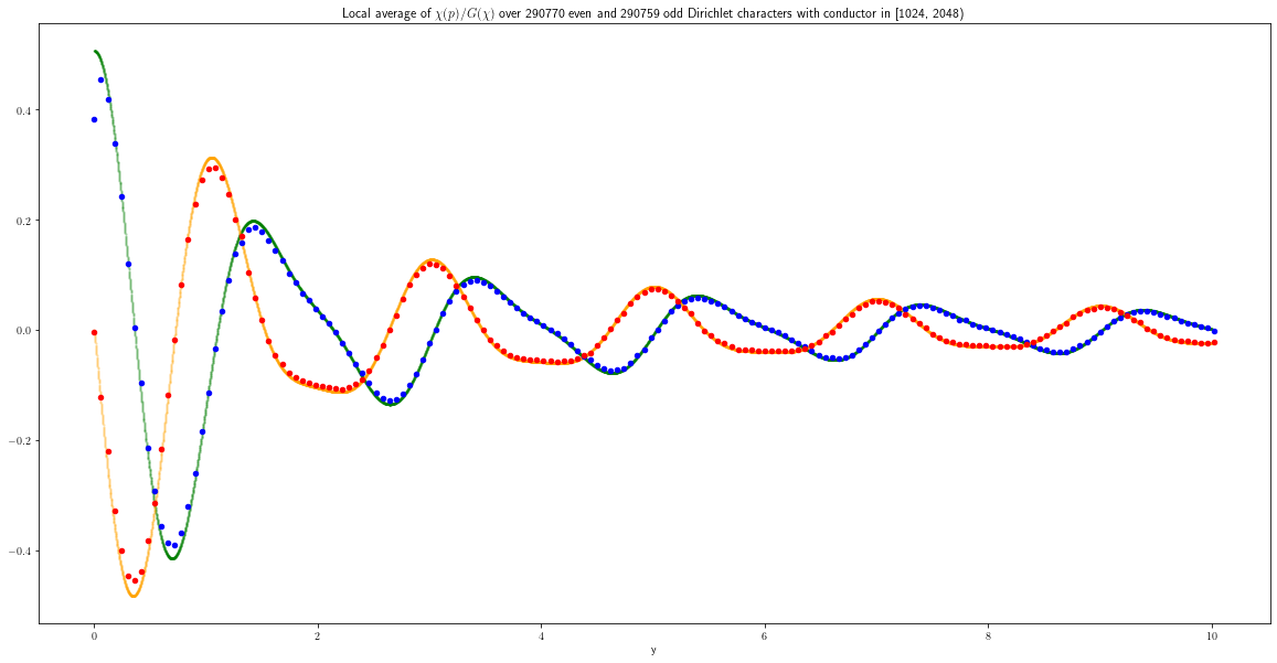
Figure 6. Plot of $T_{\pm}(y,1024,2)$ for $0\leq y\leq 10$ with $+$ in blue and (the imaginary part of) $-$ in red. We also show $\frac{5}{\pi^{2}}\int_{1}^{2}\cos\left(\frac{2\pi y}{x}\right)dx$ in green and $-\frac{5}{\pi^{2}}\int_{1}^{2}\sin\left(\frac{2\pi y}{x}\right)dx$ in orange.

Proof.

We will prove the case of $T_{+}(y,X,c)$, and simply note that $T_{-}(y,X,c)$ is similar. Applying equations (2.17), (6.1), and (6.11) to equation (6.8), we deduce

(6.23) $$\begin{split}\lim_{X\to\infty}T_{+}(y,X,\delta)&=\lim_{X\to\infty}\frac{1}{X}\sum_{\begin{subarray}{c}N\in[X,cX]\\ N\not\equiv 2\bmod 4\end{subarray}}\frac{\phi(N)}{N}\cos\left(\frac{2\pi yX}{N}\right)-\lim_{X\rightarrow\infty}E_{+}(y,X,\delta)\\ &=\lim_{X\to\infty}\frac{1}{X}\sum_{i=1}^{n}\sum_{\begin{subarray}{c}N\in I_{i}\\ N\not\equiv 2\bmod 4\end{subarray}}\frac{\phi(N)}{N}\cos\left(\frac{2\pi yX}{N}\right)-\lim_{X\rightarrow\infty}E_{+}(y,X,\delta),\end{split}$$

where, for each $X$, we put $n=\left\lceil\sqrt{X}\right\rceil$ and, for $i\in\left\{1,\dots,n\right\}$, we write

(6.24) $$I_{i}=\left[X+\frac{i-1}{n}(c-1)X,X+\frac{i}{n}(c-1)X\right).$$

Fix $\gamma\in(0,1]$ and, for each $X$, choose $i=\lceil\gamma n\rceil\in\{1,\dots,n\}$. We have

(6.25) $$\lim_{X\to\infty}\frac{i-1}{n}=\lim_{X\to\infty}\frac{i}{n}=\gamma.$$

For $N\in I_{i}$, equation (6.25) implies that

(6.26) $$\frac{1}{1+\gamma(c-1)}=\lim_{X\to\infty}\frac{X}{X+i(c-1)X/n}\leq\lim_{X\to\infty}\frac{X}{N}\leq\lim_{X\to\infty}\frac{X}{X+(i-1)(c-1)X/n}=\frac{1}{1+\gamma(c-1)}.$$

Combining equations (6.13),  (6.23), and  (6.26), we deduce

(6.27) $$\lim_{X\to\infty}T_{+}(y,X,\delta)=\lim_{X\to\infty}\frac{c-1}{\sqrt{X}}\sum_{i=1}^{n}\cos\left(\frac{2\pi y}{1+\gamma(c-1)}\right)\frac{1}{(c-1)\sqrt{X}}\sum_{\begin{subarray}{c}N\in I_{i}\\ N\not\equiv 2\bmod 4\end{subarray}}\frac{\phi(N)}{N}.$$

Using  (6.15) and (6.27), we are led to

(6.28) $$\lim_{X\to\infty}T_{+}(y,X,\delta)=\lim_{n\to\infty}\frac{c-1}{n}\sum_{i=1}^{n}\frac{5}{\pi^{2}}\cos\left(\frac{2\pi y}{1+i(c-1)/n}\right).$$

Now equation (6.22) follows upon recognising equation (6.28) as a Riemann sum. ∎

6.1.3. Short intervals

We first prove the following theorem, which is visualised in Figure 7.

Theorem 6.5.

If $\delta\in(0,1)$ and $y\in\mathbb{R}_{>0}$, then

(6.29) $$\lim_{X\rightarrow\infty}\widetilde{T}_{\pm}(y,X,\delta)=\begin{cases}\frac{5}{\pi^{2}}\cos(2\pi y),&\text{ if $+$},\\ -i\frac{5}{\pi^{2}}\sin(2\pi y),&\text{ if $-$}.\end{cases}$$

Figure 7. Plot of $\widetilde{T}_{\pm}(y,2002,0.51)$ for $0\leq y\leq 2$ with $+$ in blue and (imaginary part of) $-$ in red. We also show $\frac{5}{\pi^{2}}\cos(2\pi y)$ in green and $\frac{5}{\pi^{2}}\sin(2\pi y)$ in orange.

Proof.

We will prove the case of $\widetilde{T}_{+}(y,X,\delta)$ and simply note that $\widetilde{T}_{-}(y,X,\delta)$ is similar. Mimicking the proof of equation (1.4) leads to

(6.30) $$\lim_{X\to\infty}\widetilde{T}_{+}(y,X,\delta)=\lim_{X\to\infty}\frac{\cos(2\pi y)}{X^{\delta}}\sum_{\begin{subarray}{c}N\in[X,X+X^{\delta}]\\ N\not\equiv 2\text{ mod }4\end{subarray}}\frac{\phi(N)}{N}.$$

In light of equation (6.30), the result follows from Lemma 6.3. ∎

We next obtain an extension of equation (1.4) by considering a set of special conductors specified as follows. Let $S$ denote the set of positive integers that are not congruent to $2$ mod $4$ and are either prime or squarefull. By equation (6.10), this is precisely the set $S$ of integers such that, if $N\in S$, then

(6.31) $$\sum_{\mathcal{I}_{\pm}(N)}\tau(\overline{\chi})\chi(p)=0,\ \ (N\in S).$$

Using equations (2.17) and (6.31), we deduce that, for $N\in S$, equation (6.8) reduces to

(6.32) $$\sum_{\chi\in\mathcal{D}_{\pm}(N)}\frac{\chi(p)}{\tau(\chi)}=\frac{\phi(N)}{N}\cos\left(\frac{2\pi p}{N}\right),\ \ (N\in S).$$

Now define

(6.33) $$f(X)=\sum_{\begin{subarray}{c}N\leq X\\ N\in S\end{subarray}}\frac{\phi(N)}{N},$$

and consider

(6.34) $$\widetilde{Q}_{\pm}^{S}(y,X,\delta)=\frac{1}{f(X+X^{\delta})-f(X)}\sum_{\begin{subarray}{c}N\in[X,X+X^{\delta}]\\ N\in S\end{subarray}}\sum_{\chi\in\mathcal{D}_{\pm}(N)}\frac{\chi(\lceil yX\rceil^{p})}{\tau(\chi)}.$$

This leads to the following corollary.

Corollary 6.6.

Under the Riemann Hypothesis, if $\delta\in(\frac{1}{2},1)$ and $y\in\mathbb{R}_{>0}$, then

(6.35) $$\lim_{X\rightarrow\infty}\widetilde{Q}^{S}_{\pm}(y,X,\delta)=\begin{cases}\cos(2\pi y),&\text{ if $+$},\\ -i\sin(2\pi y),&\text{ if $-$}.\end{cases}$$

Proof.

We prove the case of $\widetilde{Q}_{+}^{S}(y,X,\delta)$ and simply note that $\widetilde{Q}_{-}^{S}(y,X,\delta)$ is similar. Using equation (6.32) and mimicking the proof of equation (1.4) yields

(6.36) $$\lim_{X\to\infty}\widetilde{Q}^{S}_{+}(y,X,\delta)=\lim_{X\to\infty}\frac{\cos(2\pi y)}{f(X+X^{\delta})-f(X)}\sum_{\begin{subarray}{c}N\in[X,X+X^{\delta}]\\ N\in S\end{subarray}}\frac{\phi(N)}{N},$$

from which the result follows by equation (6.33). ∎

6.2. Zubrilina density for $\left(\frac{d}{\cdot}\right)$

Using the techniques from Section 4, we may investigate the following variation of equation (1.5):

(6.37) $$\begin{split}M^{\dagger}_{\Phi}(y,X,\delta)&=\frac{\log X}{X^{1+\delta}}\sum_{\begin{subarray}{c}p\in[yX,yX+X^{\delta}]\\ p\text{ prime}\end{subarray}}\left(\sum_{\begin{subarray}{c}d\in\mathcal{F}\\ d\equiv 1\bmod 4\end{subarray}}\Phi\left(\frac{d}{X}\right)\chi_{d}(p)+\sum_{\begin{subarray}{c}4d\in\mathcal{F}\\ d\equiv 3\bmod 4\end{subarray}}\Phi\left(\frac{d}{X}\right)\chi_{4d}(p)\right)\sqrt{p}\\ &=\frac{\log X}{X^{1+\delta}}\sum_{\begin{subarray}{c}p\in[yX,yX+X^{\delta}]\\ p\text{ prime}\end{subarray}}\sum_{\begin{subarray}{c}d\in\mathcal{F}\end{subarray}}\Phi\left(\frac{d}{X}\right)\left(\frac{d}{p}\right)\sqrt{p}.\end{split}$$

We note that $M^{{\dagger}}_{\Phi}(y,X,\delta)$ involves $\left(\frac{d}{\cdot}\right)$, whereas $M_{\Phi}(y,X,\delta)$ involves $\left(\frac{8d}{\cdot}\right)$. For plots of the function $M^{{\dagger}}_{\Phi}(y,X,\delta)$, see Figure 8.

Figure 8. Let $$\Phi_{+}(x)=\mathbbm{1}_{(1,2)}(x)\exp(\tfrac{-1}{1-4(x-1.5)^{2}})\quad\text{ and }\quad\Phi_{-}(x)=\mathbbm{1}_{(-2,-1)}(x)\exp(\tfrac{-1}{1-4(-x-1.5)^{2}}).$$ We plot $M^{{\dagger}}_{\Phi_{\pm}}(y,2^{19},2/3)$ for $y\in[0,2]$ with $+$ in blue (resp. $-$ in red), and the right hand side of equation (6.38) in green (resp. orange)

In this section, we calculate the following limit which yields Zubrilina density associated to $M^{{\dagger}}_{\Phi}(y,X,\delta)$:

Corollary 6.7.

Fix $y\in\mathbb{R}_{>0}$. If $\delta\in(\frac{1}{2},1)$ and $\Phi\geq 0$ is a smooth Schwartz function with compact support, then, assuming the Generalized Riemann Hypothesis, we have

(6.38) $$M^{\dagger}_{\Phi}(y,\delta)\coloneqq\lim_{X\to\infty}M^{\dagger}_{\Phi}(y,X,\delta)=\frac{1}{2}\sum_{\begin{subarray}{c}a=1\\ (a,2)=1\end{subarray}}^{\infty}\frac{\mu(a)}{a^{2}}\sum_{m=1}^{\infty}\widetilde{\Phi}\left(\frac{m^{2}}{a^{2}y}\right).$$

Proof.

Combining equation (2.25) with equation (6.37), we get

(6.39) $$M^{\dagger}_{\Phi,A}(y,X,\delta)=\frac{\log X}{X^{\delta}}\sum_{\begin{subarray}{c}p\in[yX,yX+X^{\delta}]\\ p\text{ prime}\end{subarray}}\frac{1}{2}\left(\frac{2}{p}\right)\sum_{\begin{subarray}{c}a\leq A\\ (a,2p)=1\end{subarray}}\frac{\mu(a)}{a^{2}}\sum_{k\in\mathbb{Z}}(-1)^{k}\left(\frac{k}{p}\right)\widetilde{\Phi}\left(\frac{kX}{2a^{2}p}\right).$$

Following the argument in Section 4.2, we observe that terms corresponding to $2k\neq\square$ vanish in equation (6.39). On the other hand, if $2k=\square$, then writing $k=2m^{2}$ yields

(6.40) $$\sum_{\begin{subarray}{c}k\in\mathbb{Z}\\ k=\square\end{subarray}}(-1)^{k}\left(\frac{2k}{p}\right)\widetilde{\Phi}\left(\frac{kX}{2a^{2}p}\right)=\sum_{m=1}^{\infty}(-1)^{2m^{2}}\left(\frac{2m}{p}\right)^{2}\widetilde{\Phi}\left(\frac{m^{2}X}{2a^{2}p}\right)=\sum_{\begin{subarray}{c}m=1\\ (2m,p)=1\end{subarray}}^{\infty}\widetilde{\Phi}\left(\frac{m^{2}X}{a^{2}p}\right).$$

To complete the proof, we argue as in Section 4.2 with $H(w)=\widetilde{\Phi}(w^{2})$. ∎

Note that, unfolding $\widetilde{\Phi}$, we may recover the analogue of equation (1.9) for $M_{\Phi}^{{\dagger}}(y,X,\delta)$. Subsequently, one may compute the Zubrilina density for the family $\left\{\left(\frac{d}{\cdot}\right):d\in\mathcal{F}\right\}$. Following the proof in Section 5, we also obtain the following analogue of Corollary 1.3.

Corollary 6.8.

Let $\Phi$ be a Schwartz function with compact support and let $\delta\in(\frac{1}{2},1)$. Assuming the Generalized Riemann Hypothesis, we have

(6.41) $$\lim_{y\rightarrow 0^{+}}M^{{\dagger}}_{\Phi}(y,\delta)=0\quad\text{ and }\quad\lim_{y\rightarrow\infty}M^{{\dagger}}_{\Phi}(y,\delta)=-\frac{2}{\pi^{2}}\widetilde{\Phi}(0),$$

where $M^{\dagger}_{\Phi}(y,\delta)$ is defined in (6.38).

References

- [A76] T. Apostol, Introduction to Analytic Number Theory, Undergraduate Texts in Mathematics, Springer-Verlag (1976).
- [BHP] R. C. Baker, G. Harman and J. Pintz, The difference between consecutive primes II, Proc. London Math. Soc. 83 (2001), no. 3, 532–562.
- [B98] D. Bump, Automorphic forms and representations, Cambridge University Press (1998).
- [C23] A. Cowan, Murmurations and explicit formulas, arXiv:2306.10425 (2023).
- [GS07] A. Granville and K. Soundararajan, Large character sums: pretenious characters and Pólya–Vinogradov theorem, J. Amer. Math. Soc. 20 (2007), no. 2, 357–384.
- [HLO1] Y.-H. He, K.-H. Lee and T. Oliver, Machine learning the Sato–Tate conjecture, J. Symbolic Comput. 111 (2022), 61–72.
- [HLO2] Y.-H. He, K.-H. Lee and T. Oliver, Machine learning number fields, Mathematics, Computation and Geometry of Data 2 (2022), 49–66.
- [HLO3] Y.-H. He, K.-H. Lee and T. Oliver, Machine learning invariants of arithmetic curves, J. Symbolic Comput. 115 (2023), 478–491.
- [HLOP] Y.-H. He, K.-H. Lee, T. Oliver, and A. Pozdnyakov, Murmurations of elliptic curves, arXiv:2204.10140 (2022).
- [HLOPS] Y.-H. He, K.-H. Lee, T. Oliver, A. Pozdnyakov, and A. Sutherland, Murmurations of -functions, in preparation.
- [IK04] H. Iwaniec and E. Kowalski, Analytic number theory, American Mathematical Soc. (2004).
- [J10] G. 1. O. Jameson, Even and odd square-free numbers, The Mathematical Gazette. 94(529) (2010) 123-127.
- [J73] H. Jager, On the number of Dirichlet characters with modulus not exceeding x, Indagationes Mathematicae (Proceedings) 76 (1973), no. 5, 452–455.
- [N75] J. E. Nymann, On the probability that positive integers are relatively prime II, Journal of Number Theory 7 (1975), no. 4, 406–412.
- [RS94] M. Rubinstein and P. Sarnak, Chebyshev’s bias, Experimental Mathematics 3 (1994), no. 3, 173-197.
- [S23i] P. Sarnak, Root numbers and murmurations, ICERM Workshop, July 7, 2023.
- [S23ii] P. Sarnak, Letter to Sutherland and Zubrilina, August, 2023.
- [S76] L. Schoenfeld, Sharper Bounds for the Chebyshev Functions and . II. Mathematics of Computation 30 (1976), no. 134, 337–360.
- [S00] K. Soundararajan, Nonvanishing of quadratic Dirichlet -functions at s=1/2, Ann. Math. 152 (2000), no.2, 447–488.
- [Z23] N. Zubrilina, Murmurations, arXiv:2310.07681 (2023).