Indian Institute of Technology Kharagpur, Indiaanubhavdhar@kgpian.iitkgp.ac.inIndian Institute of Technology Kharagpur, Indiasoumitahait7321@gmail.com Indian Institute of Technology Kharagpur, Indiaskolay@cse.iitkgp.ac.in \Copyright \ccsdescTheory of computation Computational geometry \hideLIPIcs\EventEditorsPetr A. Golovach and Meirav Zehavi \EventNoEds2 \EventLongTitle16th International Symposium on Parameterized and Exact Computation (IPEC 2021) \EventShortTitleIPEC 2021 \EventAcronymIPEC \EventYear2021 \EventDateSeptember 8–10, 2021 \EventLocationLisbon, Portugal \EventLogo \SeriesVolume214 \ArticleNo2
Efficient Algorithms for \ESMTon Near-Convex Terminal Sets
Abstract
The \ESMTproblem takes as input a set of points in the Euclidean plane and finds the minimum length network interconnecting all the points of . In this paper, in continuation to the works of [5] and [16], we study \ESMTwhen is formed by the vertices of a pair of regular, concentric and parallel -gons. We restrict our attention to the cases where the two polygons are not very close to each other. In such cases, we show that \ESMTis polynomial-time solvable, and we describe an explicit structure of a Euclidean Steiner minimal tree for .
We also consider point sets of size where the number of input points not on the convex hull of is . We give an exact algorithm with running time for such input point sets . Note that when , our algorithm runs in single-exponential time, and when the running time is which is better than the known algorithm in [9].
We know that no FPTAS exists for \ESMTunless [6]. On the other hand FPTASes exist for \ESMTon convex point sets [14]. In this paper, we show that if the number of input points in not belonging to the convex hull of is , then an FPTAS exists for \ESMT. In contrast, we show that for any , when there are points not belonging to the convex hull of the input set, then no FPTAS can exist for \ESMTunless .
keywords:
Steiner minimal tree, Euclidean Geometry, Almost Convex point sets, FPTAS, strong NP-completenesscategory:
\relatedversion1 Introduction
The \ESMTproblem asks for a network of minimum total length interconnecting a given finite set of points in the Euclidean plane. Formally, we define the problem as follows, taken from [2]:
\ESMT Input: A set of points in the Euclidean plane Question: Find a connected plane graph such that is a subset of the vertex set , and for the edge set , is minimized over all connected plane graphs with as a vertex subset.
Note that the metric being considered is the Euclidean metric, and for any edge , denotes the Euclidean length of the edge. Here, the input set of points is often called a set of terminals, the points in are called Steiner points. A solution graph is referred to as a Euclidean Steiner minimal tree, or simply an SMT.
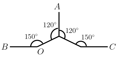
The \ESMTproblem is a classic problem in the field of Computational Geometry. The origin of the problem dates back to Fermat (1601-1665) who proposed the problem of finding a point in the plane such that the sum of its distance from three given points is minimized. This is equivalent to finding the location of the Steiner point when given three terminals as input. Torricelli proposed a geometric solution to this special case of 3 terminal points. The idea was to construct equilateral triangles outside on all three sides of the triangle formed by the terminals, and draw their circumcircles. The three circles meet at a single point, which is our required Steiner point. This point came to be known as the Torricelli point. When one of the angles in the triangle is at least , the minimizing point coincides with the obtuse angle vertex of the triangle. In this case, the Torricelli point lies outside the triangle and no longer minimizes the sum of distances from the vertices. However, when vertices of polygons with more than 3 sides are considered as a set of terminals, a solution to the Fermat problem does not in general lead to a solution to the \ESMTproblem. For a more detailed survey on the history of the problem, please refer to [2, 9]. For convenience, we refer to the \ESMTproblem as ESMT.
ESMT is NP-hard. In [6], Garey et al. prove a discrete version of the problem (Discrete ESMT) to be strongly NP-complete via a reduction from the Exact Cover by 3-Sets (X3C) problem. Although it is not known if the ESMT problem is in NP, it is at least as hard as any NP-complete problem. So, we do not expect a polynomial time algorithm for it. A recursive method using only Euclidean constructions was given by Melzak in [11] for constructing all the Steiner minimal trees for any set of points in the plane by constructing full Steiner trees of subsets of the points. Full Steiner trees are interconnecting trees having the maximum number of newly introduced points (Steiner points) where all internal junctions are of degree . Hwang improved the running time of Melzak’s original exponential algorithm for full Steiner tree construction to linear time in [8]. Using this, we can construct an Euclidean Steiner minimal tree in time for any set of points. This was the first algorithm for \ESMT. The problem is known to be NP-hard even if all the terminals lie on two parallel straight lines, or on a bent line segment where the bend has an angle of less than [13]. Since the above sets of terminals all lie on the boundary of a convex polygon (or, are in convex position), this shows that ESMT is NP-hard when restricted to a set of points that are in weakly convex position.
Although the ESMT problem is NP-hard, there are certain arrangements of points in the plane for which the Euclidean Steiner minimal tree can be computed efficiently, say in polynomial time. One such arrangement is placing the points on the vertices of a regular polygon. This case was solved by Du et al. [5]. Their work gives exact topologies of the Euclidean Steiner minimal trees. Weng et al. [16] generalized the problem by incorporating the centre point of the regular polygon as part of the terminal set, along with the vertices. This case was also found to be polynomial time solvable.
Tractability in the form of approximation algorithms for ESMT has been extensively studied. It was proved in [6] that a fully polynomial time approximation scheme (FPTAS) cannot exist for this problem unless . However, we do have an FPTAS when the terminals are in convex position [14]. Arora’s celebrated polynomial time approximation scheme (PTAS) for the ESMT and other related problems is described in [1]. Around the same time, Rao and Smith gave an efficient polynomial time approximation scheme (EPTAS) in [12]. In recent years, an EPTAS with an improved running time was designed by Kisfaludi-Bak et al. [10].
Our Results.
In this paper, we first extend the work of [5] and [16]. We state this problem as ESMT on -Concentric Parallel Regular -gons.
Definition 1.1 (-Concentric Parallel Regular -gons).
-Concentric Parallel Regular -gons are regular -gons that are concentric and where the corresponding sides of polygons are parallel to each other.
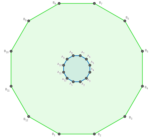
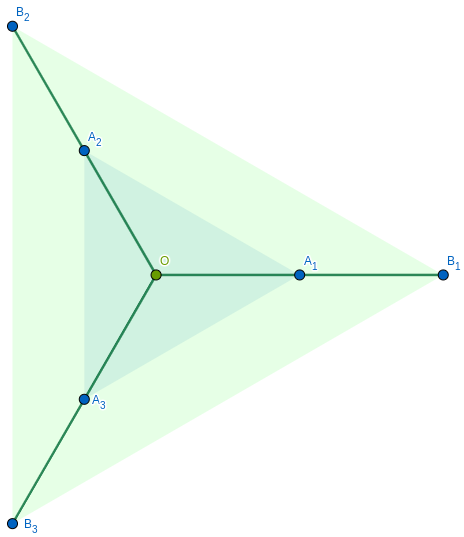
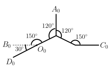
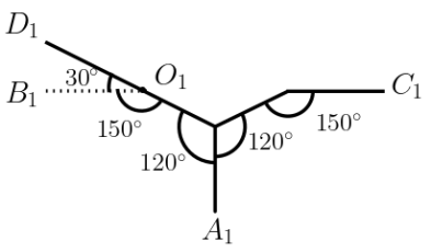
Please refer to Figure 1(a) for an example of a -Concentric Parallel Regular -gon. We call -Concentric Parallel Regular -gons as -CPR -gons for short.
We consider terminal sets where the terminals are placed on the vertices of -CPR -gons. In the case of , the -gon with the smaller side length will be called the inner -gon and the other -gon will be called the outer -gon. Also, let be the side length of the inner -gon, and be the side length of the outer -gon. We define and refer to it as the aspect ratio of the two regular polygons. In Section 3, we derive the exact structures of the SMTs for -CPR -gons when the aspect ratio of the two polygons is greater than and .
Next, we consider ESMT on an -Almost Convex Point Set.
Definition 1.2 (-Almost Convex Point Set).
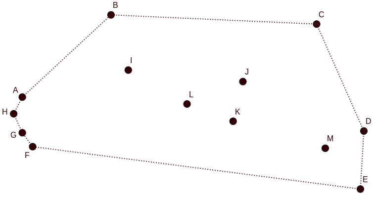
An -Almost Convex Point Set is a set of points in the Euclidean plane such that there is a partition where forms the convex hull of and .
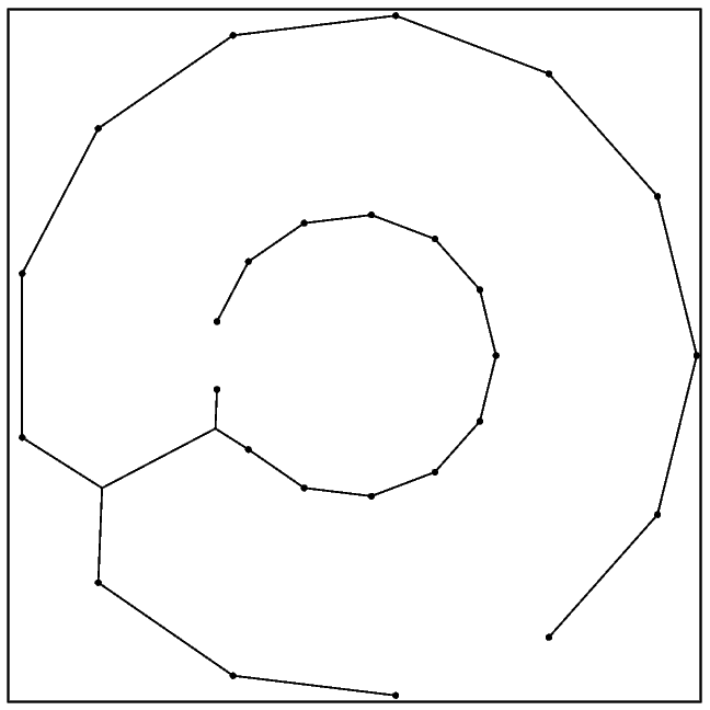
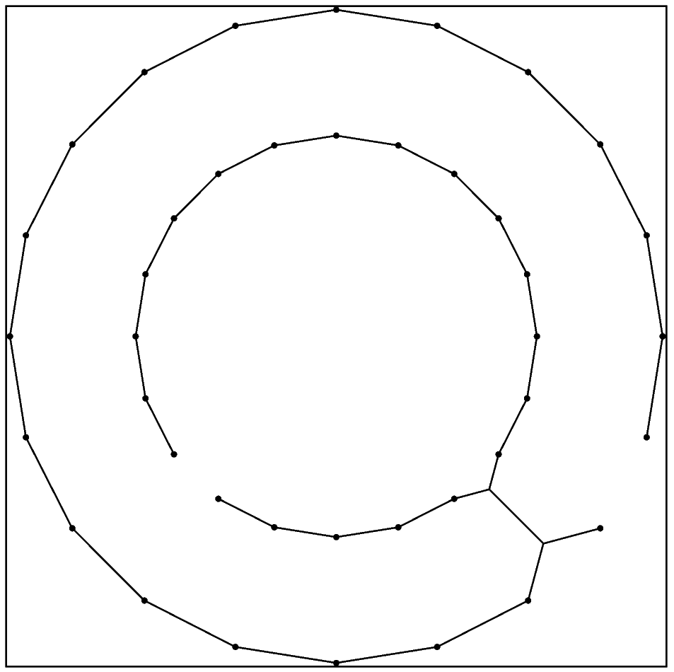
Please refer to Figure 1(b) for an example of a -Almost Convex Set of points. In Section 4, we give an exact algorithm for ESMT on -Almost Convex Sets of terminals. The running time of this algorithm is . Thus, when , then our algorithm runs in time, and when then the running time is . This is an improvement on the best known algorithm for the general case [9].
Next, for , we give an FPTAS in Section 5.1. On the other hand in Section 5.2 we show that, for all , when , there cannot exist any FPTAS unless .
2 Preliminaries
Notations.
For a given positive integer , the set of integers is denoted for short as . Given a graph , the vertex set is denoted as and the edge set as . Given two graphs and , denotes the graph where and .
In this paper, a regular -gon is denoted by or . For convenience, we define , , and . We use the notation to denote the polygon and to denote the polygon . For any regular polygon , the circumcircle of the polygon is denoted as . Given any -vertex polygon in the Euclidean plane with vertices , and interval in is a subset of consecutive vertices , , also denoted as . Here is considered the starting vertex of the interval and the ending vertex. For any , in the interval we will also use the notation .
Given two points , in the Euclidean plane, we denote by the Euclidean distance between and . Given a line segment in the Euclidean plane, . For two distinct points and , denotes the line containing and ; and denotes the ray originating from and containing .
When we refer to a graph in the Euclidean plane then is a set of points in the Euclidean plane, and is a subset of the family of line segments . For any tree in the Euclidean plane, we denote by the notation the value of . A path in a tree is uniquely specified by the sequence of vertices on the path; therefore, , , , …, (where and ) denotes the path starting from the vertex , going through the vertices , , …, and finally ending at . Equivalently, we can specify the same path as the path from to , since is a tree. Consider the graph such that , . Then is said to be the topology of while is said to realize the topology . Given two trees , in the Euclidean plane, is the graph where and .
Given any graph , a Steiner minimal tree or SMT for a terminal set is the minimum length connected subgraph of such that . The Steiner Minimal Tree problem on graphs takes as input a set of terminals and aims to find a minimum length SMT for . For the rest of the paper, we also refer to a Euclidean Steiner minimal tree as an SMT. Given a set of points in the Euclidean plane, the convex hull of is denoted as .
Euclidean Minimum Spanning Tree (MST).
Given a set of points in the Euclidean plane, let be a graph where and . Also, a weight function is defined such that for each edge , . The Euclidean minimum spanning tree of a set is the minimum spanning tree of the graph with edge weights . Note that a Steiner tree may have shorter length than a minimum spanning tree of the point set .
In the plane, the Euclidean minimum spanning tree is a subgraph of the Delaunay triangulation. Using this fact, the Euclidean minimum spanning tree for a given set of points in the Euclidean plane can be found in time as discussed in [15].
Properties of a Euclidean Steiner minimal tree.
A Euclidean Steiner minimal tree (SMT) has certain structural properties as given in [3]. We state them in the following Proposition.
Proposition 2.1.
Consider an SMT on terminals.
-
1.
No two edges of the SMT intersect with each other.
-
2.
Each Steiner point has degree exactly and the incident edges meet at angles. The terminals have degree at most and the incident edges form angles that are at least .
-
3.
The number of Steiner points is at most , where is the number of terminals.
A full Steiner tree (FST) is a Steiner tree (need not be minimal, but may include Steiner points) having exactly Steiner points, where is the number of terminals. In an FST, all terminals are leaves and Steiner points are interior nodes. When the length of an FST is minimized, it is called a minimum FST.
All SMTs can be decomposed into FST components such that, in each component a terminal is always a leaf. This decomposition is unique for a given SMT [9]. A topology for an FST is called a full Steiner topology and that of a Steiner tree is called a Steiner topology.
Steiner Hulls.
A Steiner hull for a given set of points is defined to be a region which is known to contain an SMT. We get the following propositions from [9].
Proposition 2.2.
For a given set of terminals, every SMT is always contained inside the convex hull of those points. Thus, the convex hull is also a Steiner hull.
The next two propositions are useful in restricting the structure of SMTs and the location of Steiner points.
Proposition 2.3 (The Lune property).
Let be any edge of an SMT. Let be the lune-shaped intersection of circles of radius centered on and . No other vertex of the SMT can lie in , except and themselves.
Proposition 2.4 (The Wedge property).
Let be any open wedge-shaped region having angle or more and containing none of the points from the input terminal set . Then contains no Steiner points from an SMT of .
Approximation Algorithms.
We define all the necessary terminology required in terms of a minimization problem, as ESMT is a minimization problem.
Definition 2.5 (Efficient Polynomial Time Approximation Scheme (EPTAS)).
An algorithm is called an efficient polynomial time approximation scheme (EPTAS) for a problem if it takes an input instance and a parameter , and outputs a solution with approximation factor for a minimization problem in time where is the input size and is any computable function.
Definition 2.6 (Fully Polynomial Time Approximation Scheme (FPTAS)).
An algorithm is called a fully polynomial time approximation scheme (FPTAS) for a problem if it takes an input instance and a parameter , and outputs a solution with approximation factor for a minimization problem in time where is the input size.
3 Polynomial cases for \ESMT
In this section, we consider the \ESMTproblem for -CPR -gons. Throughout the section, we denote the inner -gon as and the outer -gon as . First, we consider the configuration of an Euclidean Steiner minimal tree in a subsection of the annular area between and , which will form an isosceles trapezoid. Next, we consider the simple but illustrative case of . Finally we prove our result for all .
3.1 Isosceles Trapezoids and Vertical Forks
In this section, we discuss one particular Steiner topology when the terminal set is formed by the four corners of a given isosceles trapezoid. However, we will limit the discussion to only the isosceles trapezoids such that the angle between the non-parallel sides is of the form where , . The reason is that given -CPR -gons , , for and for any , the region is an isosceles trapezoid such that the angle between the non-parallel sides is of the form .
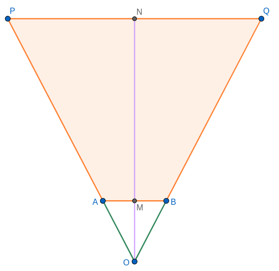
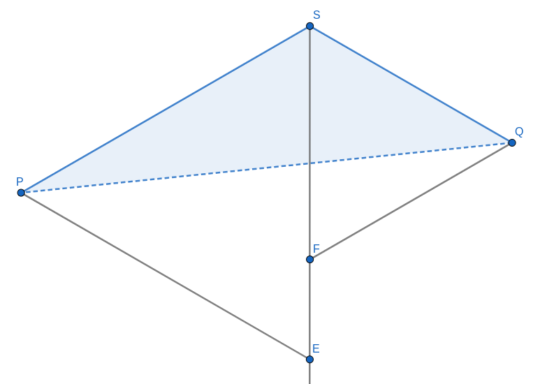
Let be an isosceles trapezoid with , as the parallel sides, and , as the non-parallel sides. Assume without loss of generality that is shorter in length than . Let and , where . For brevity, we say . Let and be the lines containing the line segments and respectively. Also let be the point of intersection of and . Further, let and be the midpoints of and respectively (as in Figure 2). As mentioned earlier, where , .
Now, we explore the following Steiner topology of the terminal set :
-
1.
and are connected to a Steiner point .
-
2.
and are connected to another Steiner point .
-
3.
and are directly connected (Please see Figure 3).
We call such a topology a vertical fork topology and the Steiner tree realising such a topology, the vertical fork. Note that in a vertical fork topology the only unknowns are the locations of the two Steiner points . Therefore, we have the vertical fork topology as , with .
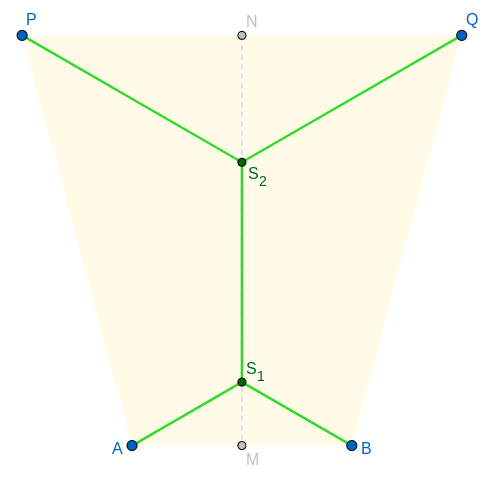
We show the existence of a vertical fork and calculate its total length in the following lemma.
Lemma 3.1.
A vertical fork can be constructed for any and for any , where
such that the length of the vertical fork
Proof 3.2.
First, we construct the Steiner points , and then prove that the construction works.
In the following construction, we describe how to find the locations of and for the vertical fork:
-
•
We construct equilateral triangles and where both points and lie outside the trapezoid .
-
•
We construct the circumcircles and of and , respectively.
-
•
Recall that is the line segment containing and . Define to be the point of intersection of and the circle distinct from ; similarly, is the point of intersection of the and distinct from . Therefore, by construction, , must lie on the same side of on , and , must lie on the same side of on . Further, by construction.
We now show that the points and indeed lie inside the line segment and the points appear in the order: , , , . We prove the following claim to serve this purpose.
Claim 1.
From 1, we get . As , lie on the same side of on and , lie on the same side of on , this implies that , lie on the line segment . Further, implies , which in turn implies that the points appear in the order: , , . .
Now, we calculate the total length of the vertical fork, :
This completes the proof of Lemma 3.1.
3.2 \ESMTfor -Concentric Parallel Regular -gons
Note that a regular -gon is an equilateral triangle and therefore, for the rest of this section we call a regular -gon as an equilateral triangle. We describe a minimal solution for \ESMTfor -CPR equilateral triangles.
Lemma 3.4.
Consider two concentric and parallel equilateral triangles and , where has side length and has side length . An SMT of is an SMT of , and has length .
Proof 3.5.
It is to be noted that the centre of both and is also the Torricelli point of both and [5]. On taking as the only Steiner point, the SMT for is [5]. However, the edges of already pass through , and . Therefore, with is also the SMT for as shown in Figure 4.
From the definition of , we have the length of the SMT for , for as
3.3 \ESMTand Large Polygons with Large Aspect Ratios
In this section, we consider the \ESMTproblem when the terminal set is formed by the vertices of -CPR -gons, namely and . As mentioned earlier, is the inner polygon and is the outer polygon of this set of -CPR -gons. In particular, we consider the case when ; for these are constant sized input instances and can be solved using any brute-force technique. We also require that the aspect ratio has a lower bound , i.e. we do not want the two polygons to have sides of very similar length. The exact value of will be clear during the description of the algorithm. Intuitively, when is very large, the SMT should look similar to what was derived in [16]. In other words, (please refer to Figure 5):
-
1.
for some , there is a vertical fork connecting the two consecutive inner polygon points with the two consecutive outer polygon points - we refer to this vertical fork as the vertical gadget for the SMT,
-
2.
the other points in are connected directly via outer polygon edges,
-
3.
the other points in are connected via inner polygon edges.
We call such a topology, a singly connected topology as in Figure 5. For the rest of this section, we consider the SMTs for a large enough aspect ratio, and show that there is an SMT that must be a realisation of a singly connected topology. We refer to an SMT for the terminal set defined by the vertices of and as the SMT for .
Without loss of generality, we consider the edge length of any side in to be . As we defined the aspect ratio to be , any side of must have a side length of . Further, we observe that for any SMT , specifying sufficiently determines the entire tree, as .
We start with the following formal definitions:
Definition 3.6.
A Steiner topology of is a singly connected topology, if it has the following structure:
-
•
A vertical gadget i.e. five edges for some , where and are newly introduced Steiner points contained in the isosceles trapezoid .
-
•
All polygon edges of excluding the edge
-
•
All polygon edges of excluding the edge
We define the notion of a path in an SMT for the vertices of and where the starting point is in and the ending point is in .
Definition 3.7.
An A-B path is a path in a Steiner tree of which starts from a vertex in and ends at a vertex in with all intermediate nodes (if any) being Steiner points.
The following Definition and Figure 6 is useful for the design of our algorithm.
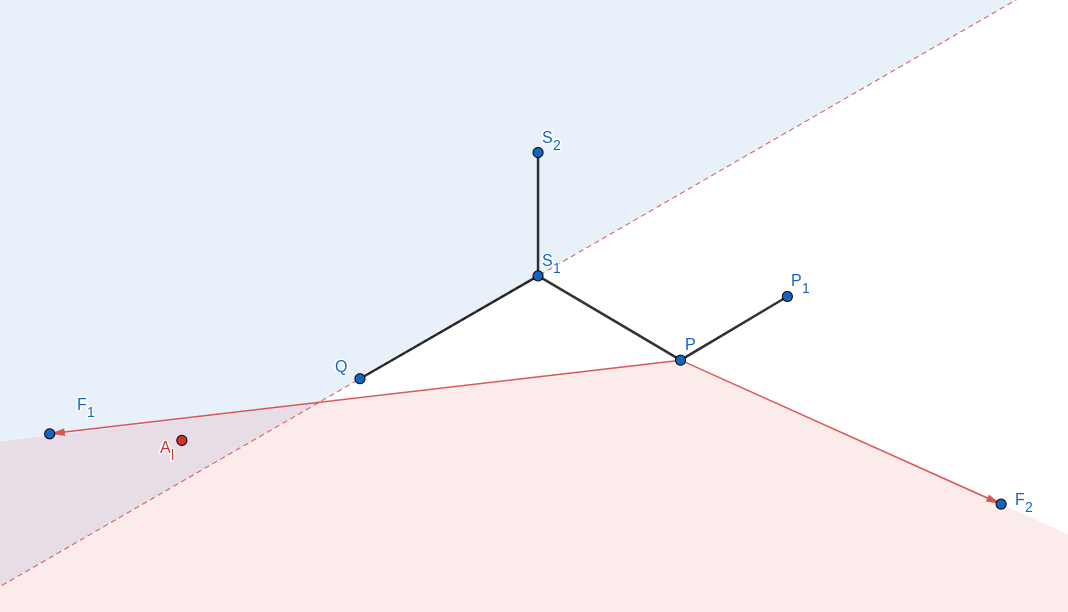
Definition 3.8.
A counter-clockwise path is a path in a Steiner tree such that for all in the counter-clockwise direction. Similarly, a clockwise path is a path in a Steiner tree such that for all in the counter-clockwise direction.
Now, we consider any Steiner point in any SMT. Let and be two neighbours of . We now prove that there is no point of the SMT inside the triangle .
Let be a Steiner point in any SMT for , with neighbours and . Then, no point of the SMT lies inside the triangle .
Proof 3.9.
By the lune property (Proposition 2.3), for any edge in an SMT, for the two circles centred at and at , respectively and both having a radius of , the intersection region does not contain any point of the SMT.
Let and be points on the internal angle bisector of , such that as shown in Figure 7. Since and are points on the angle bisector of , . Hence, triangles and are equilateral triangles.
Since is an edge in the SMT, by the lune property, the intersection of the circles centred at and , both with radius contain no point inside which is a part of the SMT. Since the lune contains the entire equilateral triangle , no point of the SMT lies inside triangle . Similarly, no point of the SMT lies inside the triangle .
Further, as , . This means . Therefore, as , and must lie outside the triangle . This implies that the triangle is covered by the union of the triangles and . As no point of the SMT lies in triangles and , triangle must contain no points of the SMT as well.
Next, we show that in an SMT for there cannot be any Steiner point, in the interior of the polygon , that is a direct neighbour of some point in the polygon .
For any SMT for , there cannot exist a Steiner point lying in the interior of the polygon such that is an edge in an SMT for some .
Proof 3.10.
For the sake of contradiction, we assume that for some SMT for there exists a Steiner point lying in the interior of the polygon such that is an edge in the SMT for some . Let be the edge such that intersects . Without loss of generality, assume that is closer to than . Therefore . This means that is the longest edge in the triangle . Therefore we can remove the edge from the SMT and replace it with either or to get another tree connecting the terminal set with a shorter total length than what we started with, which is a contradiction.
We further analyze SMTs for .
Let be the interval of consecutive vertices of lying between and (which includes ) such that is distinct from . Let be any point on the line segment . Then an SMT of is , with .
Proof 3.11.
For the sake of contradiction, assume that there exists an SMT of such that .
From [5], we know that , with (i.e. all edges of polygon except ) is an SMT of . Since , must also be an SMT of . However, can be partitioned as , where . However, as is assumed to be of shorter total length than , is a tree, containing as a vertex subset, which has a shorter total length than , contradicting the optimality of .
We proceed by showing that in any SMT for there exists at least one A-B path which is also a counter-clockwise path. Symmetrically, we also show that for any SMT for there exists another clockwise A-B path which consists of only clockwise turns. We can intuitively see that this is true because, if all clockwise paths starting at a vertex in also ended in a vertex in , there would be enough paths to form a cycle, which is not possible in a tree.
Lemma 3.12.
In any SMT for , there exists an A-B path which is also a clockwise path and there exists an A-B path which is also a counter-clockwise path.
Proof 3.13.
For the sake of contradiction, assume that for some SMT for there is no A-B path which is a counter-clockwise path. We pick an arbitrary vertex such that it is connected to at least one Steiner point (say ). We consider the counter-clockwise path, starting from and ending at the first terminal point in the counter-clockwise path. By assumption, there can be no vertex of in , hence the endpoint must be a vertex in . Let be the other endpoint of . By definition, the penultimate vertex in this counter-clockwise path must be a Steiner point, we call it . We again consider the counter-clockwise path starting from , and similarly, let be the first terminal that is encountered in this path. The penultimate vertex in this counter-clockwise path must be a Steiner point, we call it . We can repeat this procedure indefinitely to obtain as there are no counter-clockwise A-B paths. However, as has vertices, there must be a repetition of vertices among , implying the existence of a cycle in the SMT, which is a contradiction.
This symmetrically implies that there must also be a clockwise A-B path.
Our next step is to bound the number of ‘connections’ that connect the inner polygon and the outer polygon for a large aspect ratio, . As increases, the area of the annular region between the two polygons increases as well. Therefore, an increase in the number of connections would lead to a longer total length of the SMT considered. Consequently, we will prove that after a certain positive constant , for any SMT for will have a single ‘connection’ between the two polygons. Moreover, [16] gives us an evidence that as , there will indeed be a single connection connecting the outer polygon and the inner polygon for . We can formalize this notion of existence of a single ‘connection’ with the following lemma.
Lemma 3.14.
For any SMT for with and , the number of edges needed to be removed in order to disconnect and is 1, where
Proof 3.15.
For the sake of contradiction, assume that for some SMT for , there are at least two distinct edges in that SMT, which are needed to be removed in order to disconnect and . We start with a claim.
Claim 2.
A counter-clockwise A-B path in any SMT of must have an edge of length greater than .
Proof 3.16.
We consider a generic setting, where is an SMT of some set of terminal points . Let be vertex of . If be a counter-clockwise path starting from such that no edge in the counter clockwise path has a length of more than , for some . Due to Lemma 2.4 (1) of [16], we know that is contained entirely in the circle centred at with radius .
In our case, any vertex in and any vertex in are separated by the distance of at least . Therefore, by the above fact, the maximum edge length in a counter-clockwise A-B path of any SMT of must be at least . Moreover, we have . Therefore . Hence, a counter-clockwise A-B path in any SMT of must have one edge greater than . This proves the claim.
Now, for any SMT of , let be a counter-clockwise A-B path (this exists due to Lemma 3.12). From Claim 2, we know that there is an edge in , with a length greater than . On removing the edge , the SMT splits into a forest of two trees. Let the trees be and . As we assumed that there are two edges required to disconnect and , there must exist an A-B path in either or . Without loss of generality, let contain an A-B path, and hence contains at least one point from and at least one point from . Further, must contain at least one terminal point (as it must contain all terminal points in one of the sides of the removed edge ). If contains a point from , then the polygon has vertices both from and ; otherwise, if contains a point from , then the polygon has vertices both from and .
This means that either the polygon or the polygon will contain at least one node from each of and . Further, as any given vertex must be either in or in , either or must contain two consecutive vertices and such that one of them is in and the other is in . We simply connect and by the polygon edge which is of length (if ) or of length (if ), giving us back a tree containing all the terminals. However we discarded an edge of length greater than and added back an edge of length at most in this process, which means that the total length of is strictly less than the SMT we started with. This is a contradiction.
We now proceed to further investigate the connectivity of and .
Lemma 3.17.
Consider an SMT for for and . There must exist and a Steiner point , such that terminals form a path , , in the SMT and each A-B path passes through ; where
Proof 3.18.
From Lemma 3.12, we know that there exists one clockwise A-B path and one counterclockwise A-B path in any SMT of . Let a clockwise A-B path start from and a counter-clockwise A-B path start from . Further following from Lemma 3.14, as there is one edge common to all A-B paths, the clockwise A-B path from and the counter-clockwise A-B path from must share a common edge . Therefore, each A-B path must pass through and . Without loss of generality we assume that point is closer to the polygon than . This means is either a Stiener point or a terminal vertex of .
Claim 3.
is not a vertex in
Proof 3.19.
For the sake of contradiction, we assume that to be a vertex in , let in some SMT . We disconnect the edge from , which results in the formation of a forest of two trees and such that and .
must contain all vertices of and must contain all vertices of , as there would be an A-B path in the graph otherwise (contradicting that disconnects and ). We replace with the SMT of , which is also an MST (from [16]). Since all MST’s are of the same length, we choose such an MST in which is not a leaf node. This means and are edges in the chosen MST of . We now add back the edge , resulting in a connected tree of . Since we replaced the tree with an SMT of , the total length of the must not be more than the total length of the .
However, we observe that has three neighbours in , which are . However . This means either or . But due to Proposition 2.1, this cannot form an SMT. Therefore is not optimal; and hence, cannot be optimal as well. This proves the claim.
Therefore, must be a Steiner point. Let and be the neighbours of other than , such that is a clockwise turn while is a counter-clockwise turn. This means that the clockwise A-B path from passes through and the counter-clockwise A-B path from passes through . We prove that and are consecutive vertices of in some SMT of .
Claim 4.
and cannot simultaneously lie in the interior of the polygon .
Proof 3.20.
We assume for the sake of contradiction that both and lie in the interior of the polygon . On deleting the edge , the SMT of splits into two trees (rooted at ) and (rooted at ). Further, as all A-B paths pass through , all vertices of must be in whereas all vertices of must lie in . Further, must be the SMT of and must be the SMT of .
-
•
Case I: One point in lies in the interior of and the other point lies in the exterior of : This means that the edge crosses some polygon edge of , call it . Let be the intersection of and . We replace with an MST of that contains the edge (this can never lead to increase in total tree length due to [16]) and remove the line segment from . This forms a tree connecting the terminal set which has a total length smaller than the SMT we started with, which is a contradiction.
-
•
Case II: Both and lie in the interior of polygon : We further consider two cases for this:
-
–
Consider that there is at least one polygon edge of such that it does not intersect with . Then we can replace by the MST of which does not contain the edge without reducing the total edge. However, this will be a connecting tree of with a smaller total length than the tree we started with (as we had removed the edge previously), which is a contradiction.
-
–
Now, consider that all polygon edges of intersect with some edge in . Since is rooted at which lies in the interior of , there must be distinct edges crossing the polygon . However, must be the SMT of the points , which means there can be at most Steiner points other than (from Proposition 2.1). Therefore, one of these edges must have a point in as one of its endpoints, contradicting Observation 3.3.
-
–
-
•
Case III: Both and lie in the exterior of polygon : This means that the edges and intersect the polygon edges of . Further, from Observation 3.3, there cannot be any terminal inside the triangle . Hence, and must intersect the same polygon edge of (otherwise intermediate vertices from would lie in the triangle ). Let this edge be . Let and be the points of intersection of with and respectively.
We now remove the line segments and from . This results in another split into two connected trees (containing , and a subset of ) and (containing , and the remaining vertices of ).
We observe that the terminals in and form consecutive intervals of the edges in . To see why, consider the opposite, i.e. there are vertices appearing in that order in such that whereas . As and lie in the interior of , the path from to in must cross the path from to in . However, there cannot be crossing paths in the original SMT of (due to Proposition 2.1).
Let be the terminals in and the remaining terminals in are in . Again, let , be defined as:
and
From Observation 3.3, we know that is the SMT of and is the SMT of . Therefore, and . This means that , where . Further, is also a connecting tree of and as is an SMT of , then must also be an SMT with .
However, We can remove and from and add to get another connecting tree of , but with shorter total length (as from triangle inequality). This contradicts the optimality of which was derived to be an SMT of .
This proves the claim.
We proceed to prove a stronger claim regarding and .
Claim 5.
and are consecutive vertices of in any SMT of .
Proof 3.21.
We first prove that are vertices of .
From Claim 4, we know that at least one among and must not be in the interior of polygon . Without loss of generality, let it be . We now show that is a vertex of . For the sake of contradiction we assume that is not a vertex of i.e. is a Steiner point. Let and be tangents from to where are the points of tangency on . As and are tangents, . We denote the region between the tangents and which contains the all the points in as .
From any Steiner point , which lies outside , we can choose a neighbour of such that is not directed towards . Further we now show that there is one neighbour of such that is not in and .
Case I: lies in . However there must be another neighbour of not in (as ) but as is outside , we must have .
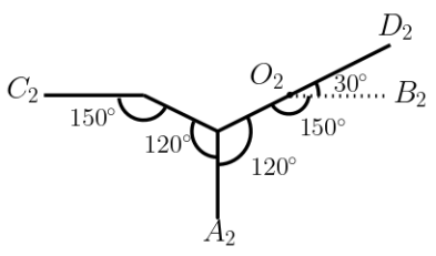
Case II: does not lie in (Figure 8). As the counter-clockwise A-B path from passes through , must be to the left of the line if the line is given a orientation from to . This means that one of the tangents from (Without loss of generality assume it to be ) intersects with the line . Therefore, taking angles in counter-clockwise order, we have:
Hence there must exist one neighbour of lying outside the , precisely in the region bounded by the rays and with .
Further we can choose a neighbour of such that is directed away from . We can continue choosing such that is directed away from the region . Moreover, the path must end at some point as it cannot end in any vertex of (since all vertices of are in ). Now, let be the path from to (which passes through and ) and let be the counter-clockwise A-B path from (passing through , and ). We observe that and are two edge disjoint A-B paths, which is a contradiction to Lemma 3.14. This proves that is indeed a vertex in . Therefore by Claim 4, does not lie inside and repeating this same argument on yields that is also a vertex of .
Now, to prove that and are consecutive vertices of , we use Observation 3.3. Observation 3.3 implies that there must not be any other point of the SMT in the triangle . This means that and must be consecutive vertices of , otherwise all polygon vertices of occurring in between and would be inside the triangle (as and ). This proves the claim.
Therefore, and are consecutive vertices of the polygon , for some such that , , is a path in the SMT, where is a Steiner point lying on all A-B paths.
Our next step is to investigate some more structural properties of an SMT for . From [5], we may guess that there would be a lot of polygon edges of both and in an SMT. We prove the following Lemma, stating that there is an SMT of which contains polygon edges of .
Lemma 3.22.
For an SMT for with aspect ratio , , let be the Steiner point such that all A-B paths pass through . Let and be vertices of which are connected to . Then, there exists an SMT of having polygon edges of other than .
Proof 3.23.
Let be any SMT of . From Lemma 3.17, we know that there exists , and such that is a Steiner point which is a part of all A-B paths, and is a path .
From , we remove the edges and and add the edge . This results in a forest of two disjoint trees and . One of these trees (say ) must contain all terminal points from and the other tree must contain all terminals from , as no more A-B paths exist after we removed the edges and . Therefore we have .
We further replace with a Euclidean minimum spanning tree of such that the edge is present in . From [5], we know that . We now remove the edge and add back the edges and which gives a connected tree of . Therefore we have:
This means must be an SMT. However, all polygon edges of polygon appearing in also appear in as well, except . Therefore, the SMT has polygon edges of the polygon .
With these set of results in hand, we can now show that there exists an SMT of following a singly connected topology. To show this, we start with any SMT for , , that satisfies all the results derived so far and transform it into a Steiner tree of singly connected topology having total length not longer than the initial Steiner tree .
Theorem 3.24.
There exists an SMT for following a singly connected topology for and , where
Proof 3.25.
Let be any SMT of which satisfies the properties of Lemma 3.22. Further, from Lemma 3.17, there is a Steiner point which lies on all A-B paths, and there are two consecutive vertices , such that , , is a path in . As satisfies the property of Lemma 3.22, has polygon edges of excluding the edge .
Let be the point in the interior of the polygon such that form an equilateral triangle. As , the common centre of and does not lie inside the triangle . Now, we modify as follows:
-
1.
Remove edges , and add edge to get the forest . We know from [9] that , and are collinear and this transformation does not change the total length. Therefore . Here, denotes the sum of the lengths of edges present in .
-
2.
Add edge and remove all polygon edges of to get . Therefore . We observe that is a tree connecting the points in .
-
3.
Let be the Torricelli point of the triangle . Let be the Steiner tree of with edges , , and other points in connected through polygon edges of the polygon . From [16], we know that is the SMT of . Therefore . Further we know that lies on the edge (as , and lie on the perpendicular bisector of and ).
-
4.
Remove edge and add edge to get . As lies on the edge , we have .
-
5.
Let be the intersection of the circumcircle of triangle (from Lemma 3.1 the intersection exists as for ). Remove the edge and add the edges and to get . Again, from [9] we know that this transformation does not change the total length. Hence . Moreover, as , we observe that form the vertices of the vertical gadget and points , , , appear in that order on the perpendicular bisector of and .
-
6.
Add back the polygon edges of which were removed in the second step to get . Therefore . We further observe that is a Steiner tree connecting the points with a singly connected topology.
Therefore we started with an arbitrary SMT and transformed it into a Steiner tree with a singly connected topology (where form the vertices of the vertical gadget) which has a total length not worse than . Hence must be an SMT of . This proves the theorem.
Remark 3.26.
Theorem 3.24 determines the exact structure of the SMT for . Further from Section 3.1 we determine the exact method to construct the two additional Steiner points in steps - note that this construction time is independent of the integer or the real number . Therefore, SMT for for and is solvable in polynomial time.
Note that the total length of any SMT for , when and , is
Further, converges to 1 very quickly with increasing (plotted in Figure 9):
| 13 | 20 | 40 | 100 | 500 | |
|---|---|---|---|---|---|
| 23.3987 | 2.6719 | 1.4574 | 1.1437 | 1.0258 |
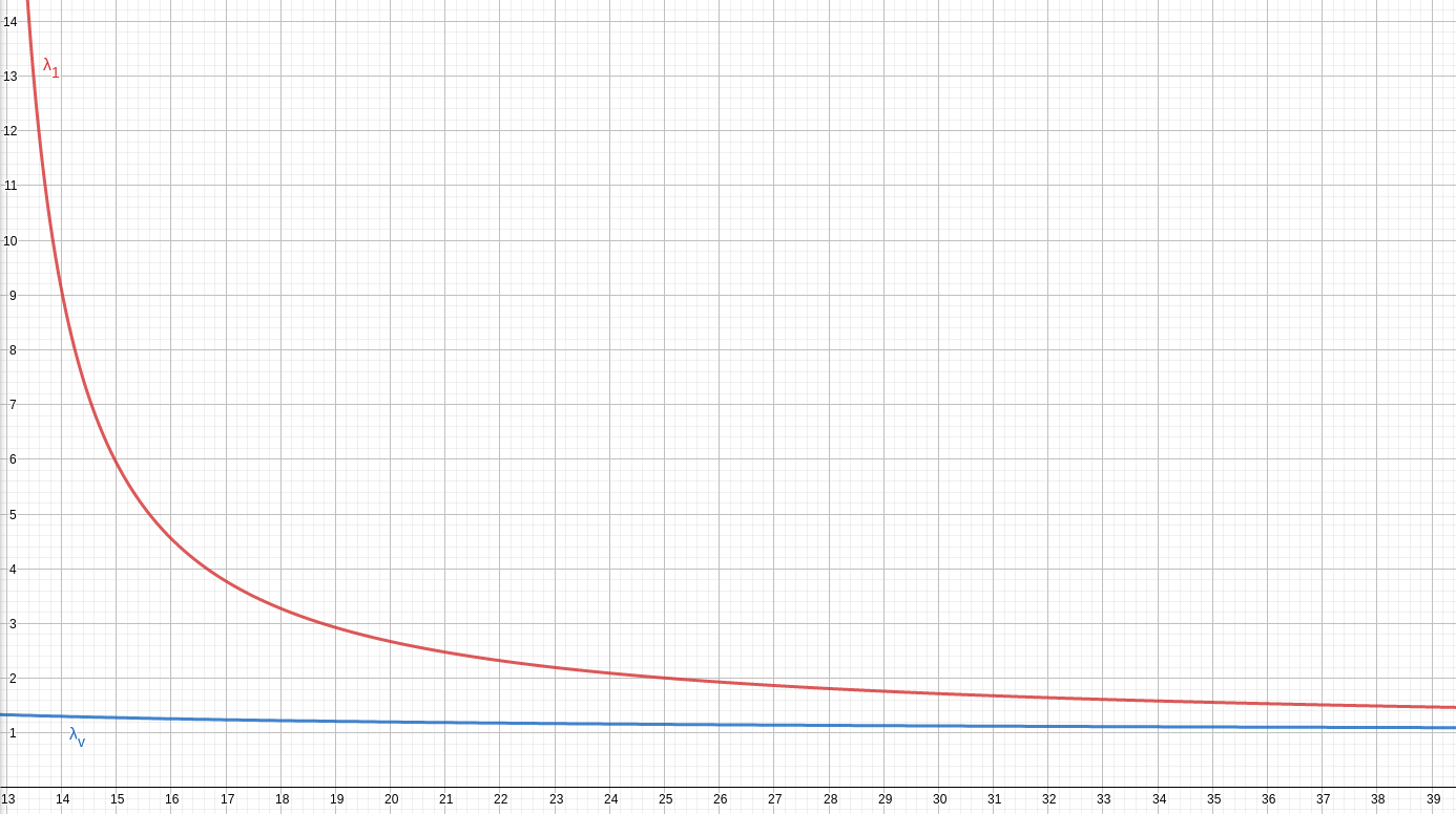
This means for large sized and for ratios that are not too small, the SMT will follow a singly connected topology.
4 \ESMTon -Almost Convex Point Sets
In this section, we design an exact algorithm for \ESMTon -Almost Convex Point Sets running in time . Note that is always true. Therefore, we are given as input a set of points in the Euclidean Plane such that can be partitioned as , where is the convex hull of and .
First, we look into some mathematical results and computational results to finally arrive at the algorithm for solving \ESMTon -Almost Convex Point Sets.
We know that the SMT of can be decomposed uniquely into one or more full Steiner subtrees, such that two full Steiner subtrees share at most one node [9]. In the following lemma, we further characterize one full Steiner subtree.
Lemma 4.1.
Let be the full Steiner decomposition of an SMT of . Then there exists a full Steiner subtree such that has at most one common node with at most one other full Steiner subtree in .
Proof 4.2.
If the SMT of is a full Steiner tree, then the statement is trivially true.
Otherwise, we assume that the SMT of has full Steiner subtrees, , . Now, for the sake of contradiction, we assume that for each full Steiner subtree there are atleast two other full Steiner subtrees and two terminals such that , . Now, let us construct a walk in the SMT of . Starting from of the full Steiner subtree , we include the path in connecting to . Note that is also contained in . Let for some . Also let . Then, we know that there is a . In , we include the path in connecting to . In general, suppose the full Steiner subtree to be considered in building the walk is which was reached via point . Then we include in the path in connecting and . Thus, we can indefinitely keep constructing the walk as for each both always exist. However, since there are full Steiner subtrees this means that there is an and two indices such that . Thus, there exists a cycle in , which implies that there is a cycle in the SMT of (contradiction). Therefore, there must be at least one full Steiner subtree that has at most one common terminal with at most one other full Steiner subtree.
Remark 4.3.
A full Steiner subtree of the SMT of has the topology of a tree. Thus, from Lemma 4.1, we conclude that a full Steiner subtree, that has at most one common terminal with at most one other full Steiner subtree, has at least one leaf of the SMT.
Definition 4.4.
Let the full Steiner subtrees, that have at most one terminal shared with at most one other full Steiner subtree, be called leaf full Steiner subtrees. Let the terminal which is shared be called the pivot of the leaf full Steiner subtree.
Lemma 4.5.
Let be a leaf full Steiner Subtree of the SMT of , with terminal points and having pivot . Deleting from the SMT of gives us an SMT of the terminal points .
Proof 4.6.
Firstly, we observe that deleting from the SMT of will indeed give us a tree, as is a leaf full Steiner subtree. Let us call this tree .
Now for the sake of contradiction, we assume that the total length of is strictly larger than the SMT of . However, this means, the total length of is strictly smaller than that of the SMT of . As is also a Steiner tree of , this contradicts the minimality of the initial SMT of .
Now we are ready to describe the algorithm. Recall that is partitioned as , where is the convex hull of and is the set of points lying in the interior of . For the sake of brevity of notations let .
Lemma 4.7.
Let be a -Almost Convex Point Set. A minimum FST of a subset of can be found in time.
Proof 4.8.
We observe that for any , forms a convex polygon with at most points lying in the interior. For , the statement of the lemma is trivially true. Hence we assume that .
From [9], the number of full Steiner topologies of is
However, we know that:
And,
Therefore, the number of full Steiner topologies of is at most . Each of these topologies can be enumerated and using Melzak’s FST Algorithm, we can also find the SMT realizing each such full Steiner topology in linear time, as given in [9]. Therefore to iterate over all topologies and find a minimum takes at most time:
Now, we find the time required for extending the results of Lemma 4.7 to all subsets of .
Lemma 4.9.
Let be a -Almost Convex Set. Computing a minimum FST for all subsets can be done in time.
Proof 4.10.
Using Lemma 4.7, we can get a minimum FST for a single subset in time. Moreover, we know that the number of subsets of that are of size is . This means that the total time to compute a minimum FST for all subsets , time taken is:
For each , we denote by a minimum FST of and by the SMT of .
Lemma 4.11.
The SMT of subset , , can be found in time, given that we have pre-computed and , .
Proof 4.12.
If was a full Steiner tree then it would be . Otherwise, contains multiple full Steiner subtrees.
Let be a leaf full Steiner subtree of with pivot . Therefore from Lemma 4.5 we have . Therefore we can iterate over all subsets and all terminals , and take the minimum-length tree among . Since we are iterating over all , and all , we are guaranteed to get and on one such iteration.
Now, as there are possibilities of and possibilities of , we have possibilities of the pair . Therefore the total time required for iterating is .
Lemma 4.13.
SMTs for all subsets , can be found in time, given that we have precomputed a minimum FST .
Proof 4.14.
Using Lemma 4.11, we can get the SMT , for a single subset in time, where . Moreover, we know that the number of subsets of that are of size is . This means that the total time to compute the SMT for all subsets , time taken is:
However, to apply Lemma 4.11 on some subset for computing , we must also have precomputed for all . This can be guaranteed by computing and , for all subsets in an increasing order of (or any order which guarantees that the subsets of are processed before ).
Finally, we state our algorithm.
Theorem 4.15.
An SMT of a -Almost Convex Set of terminals can be computed in time.
Proof 4.16.
Consider the following algorithm:
Hence we have an SMT of a -Almost Convex Point Set in time.
The above theorem gives us several improvements in special classes of inputs, based on the number of input points lying inside the convex hull of the input set, as described in the following corollary. Let there be an -Almost Convex Point Set containing points. Recall that , containing the points on the convex hull of , and . It is only possible that .
Corollary 4.17.
Let be a -Almost Convex Point Set. Then, then there is an algorithm for \ESMTsuch that, runs in time. In particular,
-
1.
When , runs in time.
-
2.
When and , runs in .
-
3.
When , runs in time.
Therefore, for , our algorithm for \ESMTdoes better on -Almost Convex Points Sets than the current best known algorithm [8].
5 Approximation Algorithms for \ESMT
The \ESMTproblem is NP-hard as shown by Garey et al. in [6]. Garey et al. also prove that there cannot be an FPTAS (fully polynomial time approximation scheme) for this problem unless . At the same time, the case when all the terminals lie on the boundary of a convex region admits an FPTAS as given in [14]. We aim to conduct a more fine-grained analysis for the problem by considering -Almost Convex Point Sets of terminals and studying the existence of FPTASes for different functions . First, we present an FPTAS for \ESMTon -Almost Convex Sets of terminals, when . Next, we prove that no FPTAS exists for the case when , where .
5.1 FPTAS for \ESMTon Cases of Almost Convex Point Sets
We first propose an algorithm for computing the SMT of a planar graph having vertices and terminals, out of which terminals lie on the outer face of and the remaining terminals lie within the boundary. Next, following the procedure in [14] we get an FPTAS for \ESMTon -Almost Convex Sets of terminals, where .
We state the following proposition from Theorem 1 in [14]:
Proposition 5.1.
Let be the vertices of any polygon in the plane, a subset of , and a tree consisting of all the vertices of (and possibly some other vertices as well) and contained entirely inside . Then on removing any edge of the tree, we get two disjoint trees , such that the vertices of in each tree form an interval in .
Using Proposition 5.1 and the Dreyfus-Wagner algorithm [4], we give an algorithm for obtaining the SMT of a planar graph .
Let represent the set of terminals lying on the outer face of and be the set of terminals lying inside the outer face of . We have , , and . Let denote the SMT in for a terminal subset . Let denote the SMT in for the terminal set , where , is the set of vertices in forming an interval from vertex to in counterclockwise direction along the outer boundary of including but excluding , , and the degree of is at least in . Let denote the SMT in for the terminal set , where , , and are as defined in the previous case, and the degree of is at most in .
Splitting the SMT at a vertex of degree at least gives rise to two smaller instances of the Steiner Minimal Tree problem on graphs.
| (1) |
where the conditions on and are , , and .
The intuition is to root the tree at an internal terminal vertex and start growing the Steiner tree from there. Observe that on removing one of the internal vertices in the tree , we get one, two or three disjoint subtrees. They induce a partition over the terminals. The terminals in in each of the subtrees form intervals in , according to Proposition 5.1. Moreover, the terminals in can be partitioned in any way, not necessarily maintaining the interval structure. This is captured in the following recurrence relation:
| (2) |
where the conditions on , , , , and are , , and and we have
| (3) |
Our aim is to compute , where . We precompute the shortest distance between all pairs of vertices. We then compute the values of and in increasing order of cardinality of subsets of vertices in and . Let denote the shortest path length between and . The base cases are for all and .
We analyse the correctness and running time of Algorithm 2.
Theorem 5.2.
Consider a planar graph on vertices and a set of terminals such that is defined as the terminals lying on the outer face of . Moreover, let . Then Algorithm 2 computes the SMT for in in time .
Proof 5.3.
Correctness of Algorithm 2. In order to prove the correctness of Algorithm 2, we need to show that the Equations 1 and 2 are valid.
In Equation 1, denotes an SMT for the terminal set , conditioned on the fact that the degree of is at least in it. Let us split the SMT at vertex into two smaller subtrees. This must also split the terminals in in two intervals and , respectively. Otherwise it would mean that the SMT has crossing edges, which is not possible. The vertices in can be present in any of the two subtrees, hence we consider all possible partitions of into two subsets and . Thus for Equation 1, . On the other hand, the expression in the RHS of Equation 1 is a tree containing the vertex subset . Since, is an SMT for the same vertex subset, in Equation 1 . Therefore, Equation 1 is valid.
For Equation 2, we take as the root of the SMT . The degree of in the SMT can be , , or . Accordingly, on removing , we will get , , or subtrees, with the condition that in each subtree the degree of is . Again, the terminals in are divided into smaller intervals , and for some satisfying . The terminals in are divided among the subtrees in any combination. The number of such intervals and partitions is equal to the degree of in . The term is obtained by minimizing across all SMTs satisfying the condition that degree of in the SMT is . Thus in Equation 2, . On the other hand, the RHS of Equation 2 given a tree containing vertices . Since is an SMT on the terminal set , in Equation 2 . Thus, Equation 2 is valid.
Running time of Algorithm 2. All pairs shortest paths can be calculated in time. The time complexity of the dynamic program has two components to it. One is due to computation of the B(.) values using Equation 1 and the other is for calculating the C(.) values using Equation 2.
-
1.
The number of computational steps for calculating using Equation 1 is of the order of the number of choices of , , , , and such that , , , , and . Each vertex in belongs to exactly one of the sets , , or . The vertices in are partitioned into three intervals, , , and . There are at most possibilities for . This gives us a running time of .
-
2.
The number of computational steps for calculating using Equation 2 is times the order of the number of choices of , , , , , , , and such that , , , , , and . Each vertex in belongs to exactly one of the sets , , or . The vertices in are partitioned into at most four intervals, , , and . There are at most possibilities for . The factor is because calculating each of the values involves minimization over at most terms. This gives us a running time of .
Thus, the time complexity of the algorithm is .
We obtain the following corollary from the above theorem.
Corollary 5.4.
Consider a planar graph on vertices and a set of terminals such that is defined by the terminals lying on the outer face of . Moreover, let and let . Then Algorithm 2 computes the SMT for in in time .
Next we state the FPTAS for \ESMTon -Almost Convex Sets of terminals. This is achieved by converting the instance of \ESMTinto an instance of Steiner Minimal Tree on graphs. The Steiner Minimal Tree problem shall be solved using Algorithm 2. For this, we use the Algorithm 2 in [14]. We restate the Algorithm 2 in [14] for our problem instance. We denote the set of terminals with .
We analyse the correctness and running time of Algorithm 3.
Theorem 5.5.
Consider a set of points such that is defined as the points lying on the convex hull of , i.e. , and . Moreover, let . Then Algorithm 3 computes a -approximate SMT for in time .
Proof 5.6.
Correctness of Algorithm 3. In order to prove the correctness of Algorithm 3, we need to show that is a -approximation of the SMT of the terminal set , and is indeed the SMT for in the complete weighted graph .
In [14], the concept of weight planar graphs is used. A graph is called weight planar if it is a non-planar graph embedded on the Euclidean plane, having non-negative edge weights, such that every pair of edges and which intersect in this embedding of , satisfy the inequality: , where is the weight of the edge between vertices and and is the length of the shortest path between vertices and . Since the edge weights of are the Euclidean distances between the points, is a weight planar graph.
From Theorem 5 of [14], we get that the SMT of a weight planar graph does not contain any crossing edges even though the input graph is non-planar. Because the SMT does not contain any crossing edges and lies completely inside the convex hull of the terminal pointset, the terminals on the outer boundary of , i.e. , follow the interval pattern as stated in Proposition 5.1. Therefore, Algorithm 2 designed for planar graphs can be applied in the case of weight planar graphs as well. So, is the SMT for in the complete weighted graph .
Finally, from Theorem 12 in [14], we get that the length of the Steiner tree obtained from Algorithm 3 is at most times the length of the SMT of , i.e. . Thus, we are done.
Running time of Algorithm 3. Constructing the convex hull takes time. The number of lattice points contained in the bounding box is . Thus, the number of vertices in the resultant graph is . The time complexity of Algorithm 2 is . This step dominates the running time resulting in the complexity of Algorithm 3 being .
Theorem 5.7.
There exists an FPTAS for \ESMTon an -Almost Convex Set of terminals, where .
Proof 5.8.
From Theorem 5.5, we get a -approximate SMT for any -Almost Convex Set of terminals in time . For , we get the running time of Algorithm 3 to be . Thus, Algorithm 3 is an FPTAS for the Euclidean Steiner Minimal Tree problem on an -Almost Convex Set of terminals.
5.2 Hardness of Approximation for \ESMTon Cases of Almost Convex Sets
In this section, we consider the \ESMTproblem on -Almost Convex Sets of terminal points, where for some . We show that this problem cannot have an FPTAS. The proof strategy is similar to that in [6]. First, we give a reduction for the problem Exact Cover by -Sets (defined below) to our problem to show that our problem is NP-hard. Next, we consider a discrete version of our problem and reduce our problem to the discrete version. The discrete version is in NP. Therefore, this chain of reductions imply that the discrete version of our problem is Strongly NP-complete and therefore cannot have an FPTAS, following from [6]. Similar to the arguments in [6], this also implies that our problem cannot have an FPTAS.
Before we describe our reductions, we take a look at the NP-hardness reduction of the \ESMTproblem from the Exact Cover by 3-Sets (X3C) problem in [6]. In the X3C problem, we are given a universe of elements and a family of -element subsets of the elements. The objective is to decide if there exists a subcollection such that: (i) the elements of are disjoint, and (ii) . The X3C problem is NP-complete [7].
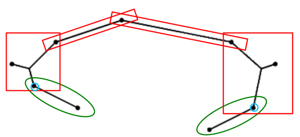
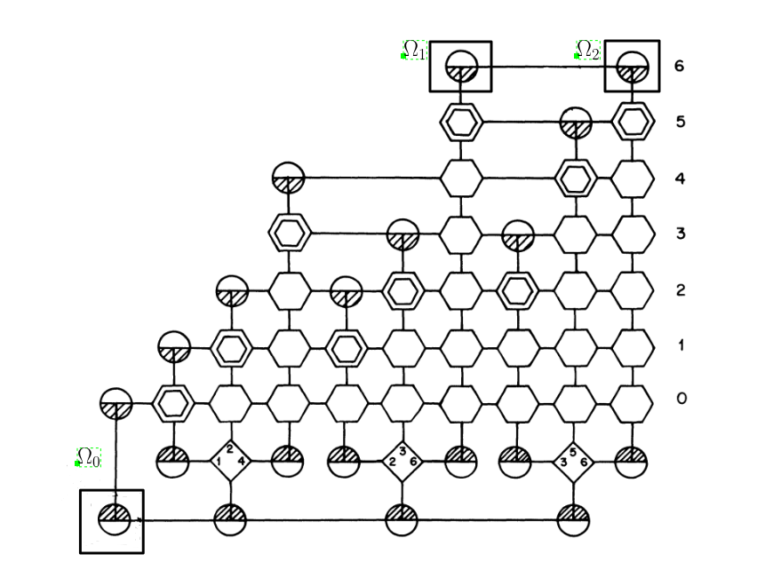
In [6], various gadgets are constructed, i.e. particular arrangements of a set of points. These are then arranged on the plane in a way corresponding to the given X3C instance. Figure 11 shows the reduced ESMT instance obtained for and (taken from [6]). The squares, hexagons (crossovers), shaded circles (terminators) and lines (rows) all represent specific arrangements of a subset of points. Let denote the reduced instance. The number of points in is bounded by a polynomial in and . Let this polynomial be , as we can assume since otherwise it trivially becomes a NO instance. Here is some constant.
We restate Theorem 1 in [6].
Proposition 5.9.
Let denote an SMT of , the instance obtained by reducing the X3C instance , and denote its length. If has an exact cover, then , otherwise , where , is the number of crossovers, i.e. hexagonal gadgets, and is a positive real-valued function of .
We extend this construction to prove NP-hardness for instances of \ESMTwhere the terminal set has points inside . Here, and is the number of terminals.
Let us call the length of a gadget to be the maximum horizontal distance between any two points in that gadget. Similarly, we define the breadth of a gadget to be the maximum vertical distance between any two points in that gadget.
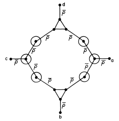
The terminator gadget used is shown in Figure 12. The straight lines represent a row of at least points separated at distances of or . The angles between them are as shown. The upward terminator has the point above the other points in the terminator, whereas the downward terminator has the point below the other points. Firstly, we adjust the number of points in the long rows, such that the length and breadth of the terminators is same as that of the hexagonal gadgets (crossovers). We can fix this length and breadth to be some constants, such that the number of points in each gadget is also bounded by some constant. In our construction, we modify the terminators , , and as shown in Figure 11 enclosed in squares. is the terminator corresponding to the first occurrence of the element in some set in and is the terminator corresponding to the last occurrence of in some set in (if there are more than one occurrences of ). If there are no occurrences of , then it is trivially a no-instance. The modified gadgets are shown in Figure 14. All the other gadgets remain unaltered.
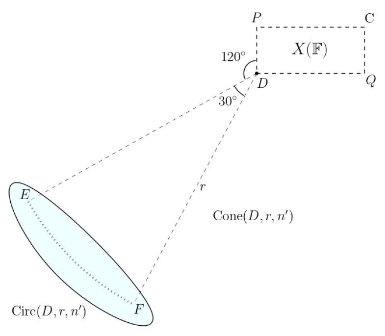
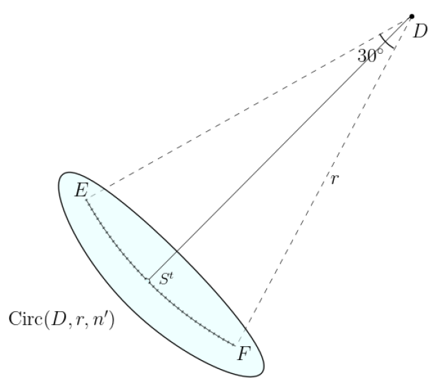
We call a set of points arranged as shown in Figure 13, as a Conic Set.
Definition 5.10.
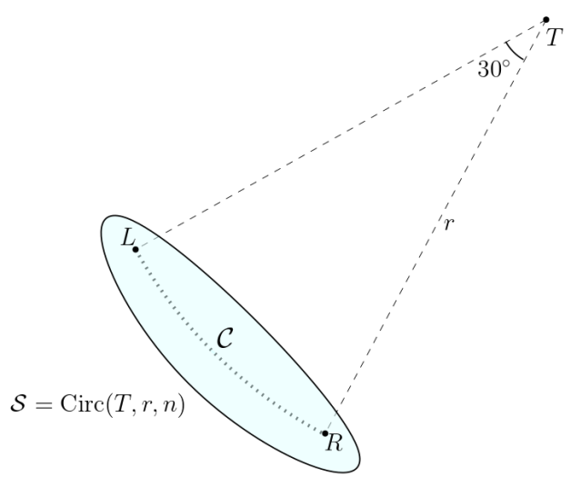
A Conic Set is a set of points consisting of a point , called the tip of the cone, and the remaining points denoted by . Let be the circle with as centre and radius . All the points in lie on , such that the angle at the tip formed by the two extreme points , i.e. in the anticlockwise direction. So, we have . The distance between any two consecutive points in is the same, say . Let the number of points in be . We denote the Conic Set as and as . We call as the left slope of the Conic Set and as the right slope of the Conic Set.
We use the Conic Set in the reduction for our problem. Now, we state the reduction of an X3C instance to an instance of \ESMT. Later, we show that the instance will satisfy the desired properties on the number of terminals inside the convex hull of the terminal set.
- Algorithm for construction of an ESMT instance from an X3C instance :
-
-
•
Reduce the input X3C instance to the points configuration according to the reduction given in [6].
-
•
Modify the terminators , , and to as shown in Figure 14 and call them , , and . Let be the smallest axis-parallel rectangle bounding after modifying the terminators, where is the bottom leftmost point of .
-
•
Take . Define and , where and and are constants. Add the , such that is the tip of the Conic Set, and the left slope makes an angle of with . The right slope also makes an angle of with .
-
•
Now we prove a few properties of the constructed instance .
Lemma 5.11.
All the points in (according to Definition 5.10) lie on the convex hull of the reduced ESMT instance constructed by Algorithm , where .
Proof 5.12.
By the construction of in Algorithm , let be the circle on which all the points in lie. If we draw a tangent to at any of the points in , then all the remaining points in the configuration lie towards one side of the tangent. We know that if we can find a line passing through a point such that all the other points in the plane lie on one side of the line, then the point lies on the convex hull of the points in the plane. Therefore, all the points in lie on the convex hull of the reduced instance .
Let us denote the convex hull of by and that of the points lying inside or on the bounding rectangle , i.e. by .
Lemma 5.13.
The reduced ESMT instance constructed by Algorithm has points inside the convex hull, where and is the total number of terminals in .
Proof 5.14.
contains all the points in by Lemma 5.11. contains points.
Now we need to analyze the number of points on . The remaining points in , i.e. must lie within the convex hull of the entire construction, i.e. . From the construction in Algorithm , no point on the connecting rows can be a part of as there is no line passing through it, which contains all terminals on one side of it. The same thing holds for the square and hexagonal gadgets as well, except the hexagonal gadgets corresponding to the last element of the last set in the family, i.e. . Thus, only the terminators and the hexagonal gadgets corresponding to the last element of contribute points to .
If we look at the arrangement of points in the terminators (modified as well as those left unchanged) and the hexagonal gadgets as shown in Figures 12 and 16, the convex hull of each of these gadgets consists of constantly many points. Therefore, the number of points each of these gadgets contribute to is bounded by some constant. The number of terminators is and the number of hexagonal gadgets corresponding to the last element of is at most . Therefore, the number of points on is as .
The instance obtained via reduction from X3C has terminators, squares, at most crossovers (hexagonal gadgets), and connecting rows of points. The number of gadgets is . Therefore, the total number of points in is . The modified terminators result in a constantly many increase in the number of points. So, we have .
Thus, the number of points inside the convex hull is and those on the convex hull is . So, the total number of terminals is , and those inside the convex hull is as .
We further prove structural properties of SMTs of the reduced instance when considering the modified gadgets , , and .
Lemma 5.15.
Consider an SMT of the ESMT instance obtained via reduction from the X3C instance as per [6]. Consider a tree on the terminal set of obtained from as follows: Consider the modified terminator gadgets as in Algorithm . For each , the edge is excluded from and the edge is included to form . is an SMT for the terminal set of .
Proof 5.16.
Consider . Due to Lemma 4 of [6], Steiner points of can only be connected to points in the triangular and square gadgets. Lemma 5 of [6] states that if there are two terminals and the distance between and does not exceed , then is an edge of . So in , for each all the points on are joined together along . Lemma 5 of [6] also holds true on modifying the terminators to . Now, we join all the points on along . This gives us the SMT for the terminal set of .
Now we focus on the structure of the SMT of . The SMT is basically the union of the SMT of the points in the bounding rectangle as stated in Lemma 5.15 and the SMT of the set of points .
is enclosed by the bounding rectangle and must lie on . We label the vertices of as in the counter-clockwise order. Let be the convex hull of all the points. By Lemma 5.11, all the points in lie on . Let and be edges in , such that .
The SMT of clearly lies inside its convex hull, . We show that the Steiner hull can be further restricted to the bounding rectangle and the convex polygon formed by the points in . For this we use Theorem 1.5 in [9], as stated below.
Proposition 5.17.
[9] Let be a Steiner hull of . By sequentially removing wedges from the remaining region, where , , are terminals but contains no other terminal, and are on the boundary and , a Steiner hull invariant to the sequence of removal is obtained.
Lemma 5.18.
The region comprising of the bounding rectangle according to Algorithm and the convex polygon formed by the set of points is a Steiner hull of .
Proof 5.19.
Firstly, let us consider the wedge . All the points are terminals, and are boundary points, and contains no other terminal. Now, is greater than the exterior angle of , which in turn is greater than . , by the construction. Therefore, . By applying Proposition 5.17, we can remove the wedge from the convex hull to get a smaller Steiner hull. This can be repeated for the wedges . The same argument can also be used to get rid of the wedges . So, we get the final Steiner hull to be the union of the bounding rectangle and the convex polygon formed by the points in .
Given the nature of the above Steiner hull, we show that we can treat and separately.
Lemma 5.20.
There is an SMT of that is the union of an SMT of and an SMT of the points in , with being common to both of them.
Proof 5.21.
According to Lemma 5.18, there is an SMT of that lies completely inside the the bounding quadrilateral and the convex polygon formed by . These two regions have as the only common point. Therefore, is an articulation point in the tree and connects these two regions. So, we have this SMT of as the union of an SMT of and an SMT of the points in .
We can identify a structure for an SMT of the points in using [16].
Lemma 5.22.
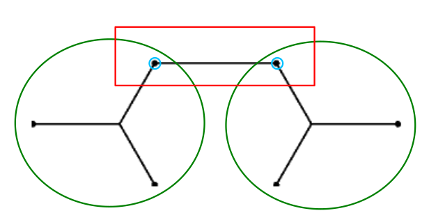
There is an SMT of the points in that is as shown in Figure 17. In the SMT, is connected to the two middle points in via a Steiner point . The other points in are connected along the circumference.
Proof 5.23.
The number of points in is . We can take the constant factor to be large enough so that . If we complete the regular polygon on having as a subset of its vertices, then it contains more than vertices and along with the centre has a SMT with structure given in [16].
Let the Steiner tree for as shown in Figure 17 be denoted by . If this is not minimal, then there exists another Steiner tree such that . Then we can replace by in the SMT of the regular polygon and its centre to get a shorter Steiner tree. This contradicts the minimality of the structure given in [16]. Therefore, the SMT of follows the structure in Figure 17.
Finally, we prove the NP-hardness of \ESMTon -Almost Convex Sets of terminals, when for some .
Theorem 5.24.
Let denote an SMT of and denote its length. If has an exact cover, then , otherwise , where is the number of crossovers, i.e. hexagonal gadgets, and is a positive real-valued function of as stated in Proposition 5.9.
Proof 5.25.
From Lemma 5.20, we have . From Lemma 5.22, we can compute the length of as a function of , , and . Finally, using Proposition 5.9 we get the required reduction.
Since it is not known if the ESMT problem is in NP, Garey et al. [6] show the NP-completeness of a related problem called the Discrete Euclidean Steiner Minimal Tree (DESMT) problem, which is in NP. We define the DESMT problem as given in [6]. The DESMT problem takes as input a set of integer-coordinate points in the plane and a positive integer , and asks if there exists a set of integer-coordinate points such that some spanning tree for satisfies , where , i.e. we round up the length of each edge to the least integer not less than it.
In order to show that DESMT is NP-hard, the same reduction as that of the ESMT problem can be used, followed by scaling and rounding the coordinates of the points. Theorem 4 of [6] proves that the DESMT problem is NP-Complete. Moreover, since it is Strongly NP-Complete, the DESMT problem does not admit any FPTAS. Finally in Theorem 5 of [6], Garey et al. show that as a consequence, the ESMT problem does not have any FPTAS as well.
Now we show that the DESMT problem is NP-hard even on -Almost Convex Sets of terminals, when and where .
In Section 7 of [6], the reduced instance of ESMT is converted into an instance of DESMT. The conversion is as follows:
, where .
We apply a similar conversion to the reduced ESMT instance , to convert it into a DESMT instance of an -Almost Convex Set. The conversion goes as follows:
, where .
The next two lemmas establish the validity of as an instance of DESMT and the upper bounds on the size of the constructed instance. Note that the reduction from X3C followed by the conversion can be done in polynomial time.
Lemma 5.26.
The instance constructed above is a valid DESMT instance.
Proof 5.27.
All the points in have integer coordinates according to the conversion stated above. So, it is a DESMT instance.
Lemma 5.28.
The reduced DESMT instance has distinct points, where .
Proof 5.29.
The minimum distance between any two points in is that between two consecutive points of , which is . Recall Lemma 5.13 which establishes that . So, the minimum distance between any two points in is . Because of the substantial distance obtained between points after scaling, the rounding will not cause any distinct points of to coincide. Therefore, the number of points remains unchanged, i.e. .
Now we present the following lemma for the constructed DESMT instance analogous to Lemma 5.13 for the ESMT instance .
Lemma 5.30.
The reduced DESMT instance constructed is an -Almost Convex Set, where .
Proof 5.31.
From Lemma 5.13, we know that the reduced ESMT instance has points inside its convex hull , and . The number of points after conversion remains the same by Lemma 5.28. We need to show that after conversion, except for the points of gadgets, no other points inside the convex hull lie on the new convex hull . The number of points in each of the anomalous gadgets are constant in number, and hence not too many points from the interior of can lie on .
After conversion, all the points on a horizontal connecting row have the same -coordinate, as they initially had the same -coordinate and therefore undergo the same transformation. Thus, all the points on a horizontal connecting row still lie on a horizontal line segment in . Similarly, all the points on a vertical connecting row still lie on a vertical line segment in . This implies that none of the points on the connecting rows can be a part of as there can be no line passing through them that also contains all terminal points on one side of it.
The same thing holds for the square and hexagonal gadgets (crossovers) as well, except the hexagonal gadgets placed at the beginning or end of any row. This is because all the points which are a part of these square and hexagon gadgets are surrounded by connecting row points all four sides, above, below, left and right. So again, only the terminators and the hexagonal gadgets appearing at the beginning or end of any row contribute to .
Now, since we had adjusted the number of points in the long rows of the terminators and hexagonal gadgets such that their lengths and breadths are some constants, the number of points in each of the terminators and hexagonal gadgets can be bounded by some constant as the minimum distance between any two consecutive points on the long rows or standard rows is at least . Therefore, each of these gadgets contribute some constantly many points to .
As we have seen in Lemma 5.13, the number of terminators is and the number of hexagonal gadgets corresponding to the beginning or end of any row is at most . Therefore, the number of points contributed by the terminators and the hexagonal gadgets placed at the beginning or the end of any row, to is , as . Even if all the points in lie on the new convex hull , we have points inside it. Thus we are done.
We get the following theorem from Lemmas 5.26, 5.28 and 5.30.
Theorem 5.32.
The instance constructed is a valid DESMT instance on an -Almost Convex Set, where .
Following Theorems 3 and 4 in [6], we get that the DESMT problem is NP-Complete for -Almost Convex Sets, where is the total number of terminals. Since we get the reduced instance from the X3C instance , the DESMT problem is strongly NP-complete for -Almost Convex Sets, and does not admit any FPTAS.
Using Theorem 5 of [6], we get that if the ESMT problem has an FPTAS, then the X3C problem can be solved in polynomial time. The Theorem also applies for our case of -Almost Convex Sets. Therefore, we get the following theorem,
Theorem 5.33.
There does not exist any FPTAS for the ESMT problem on -Almost Convex Sets of terminals, where and , unless .
6 Conclusion
In this paper, we first study ESMT on vertices of -CPR -gons and design a polynomial time algorithm. It remains open to design a polynomial time algorithm for ESMT on -CPR -gons, or show NP-hardness for the problem. Next, we study the problem on -Almost Convex Sets of terminals. For this NP-hard problem, we obtain an algorithm that runs in time. We also design an FPTAS when . On the other hand, we show that there cannot be an FPTAS if for any , unless . The question of existence of FPTASes when is a polylogarithmic function remains open.
References
- [1] Sanjeev Arora. Polynomial time approximation schemes for Euclidean traveling salesman and other geometric problems. Journal of the ACM (JACM), 45(5):753–782, 1998.
- [2] Marcus Brazil, Ronald L Graham, Doreen A Thomas, and Martin Zachariasen. On the history of the Euclidean Steiner tree problem. Archive for history of exact sciences, 68(3):327–354, 2014.
- [3] EJ Cockayne. On the Steiner problem. Canadian Mathematical Bulletin, 10(3):431–450, 1967.
- [4] Stuart E Dreyfus and Robert A Wagner. The Steiner problem in graphs. Networks, 1(3):195–207, 1971.
- [5] Ding-Zhu Du, Frank K. Hwang, and JF Weng. Steiner minimal trees for regular polygons. Discrete & Computational Geometry, 2(1):65–84, 1987.
- [6] Michael R Garey, Ronald L Graham, and David S Johnson. The complexity of computing Steiner minimal trees. SIAM Journal on Applied Mathematics, 32(4):835–859, 1977.
- [7] Michael R Garey and David S Johnson. Computers and intractability, volume 174. freeman San Francisco, 1979.
- [8] FK Hwang. A linear time algorithm for full Steiner trees. Operations Research Letters, 4(5):235–237, 1986.
- [9] FK Hwang, DS Richards, and P Winter. The Steiner tree problem. Annals of Discrete Mathematics series, vol. 53, 1992.
- [10] Sándor Kisfaludi-Bak, Jesper Nederlof, and Karol Węgrzycki. A gap-ETH-tight approximation scheme for Euclidean TSP. In 2021 IEEE 62nd Annual Symposium on Foundations of Computer Science (FOCS), pages 351–362. IEEE, 2022.
- [11] Zdzislaw Alexander Melzak. On the problem of Steiner. Canadian Mathematical Bulletin, 4(2):143–148, 1961.
- [12] Satish B Rao and Warren D Smith. Approximating geometrical graphs via “spanners” and “banyans”. In Proceedings of the thirtieth annual ACM symposium on Theory of computing, pages 540–550, 1998.
- [13] J Hyam Rubinstein, Doreen A Thomas, and Nicholas C Wormald. Steiner trees for terminals constrained to curves. SIAM Journal on Discrete Mathematics, 10(1):1–17, 1997.
- [14] J Scott Provan. Convexity and the Steiner tree problem. Networks, 18(1):55–72, 1988.
- [15] Michael Ian Shamos and Dan Hoey. Closest-point problems. 16th Annual Symposium on Foundations of Computer Science (sfcs 1975), pages 151–162, 1975.
- [16] Jia Feng Weng and Raymond Sydney Booth. Steiner minimal trees on regular polygons with centre. Discrete Mathematics, 141(1-3):259–274, 1995.