Exact Conditions for Ensemble Density Functional Theory

Abstract

Ensemble density functional theory (EDFT) is a promising alternative to time-dependent density functional theory for computing electronic excitation energies. Using coordinate scaling, we prove several fundamental exact conditions in EDFT, and illustrate them on the exact singlet bi-ensemble of the Hubbard dimer. Several approximations violate these conditions and some ground-state conditions from quantum chemistry do not generalize to EDFT. The strong-correlation limit is derived for the dimer, revealing weight-dependent derivative discontinuities in EDFT.

Sophisticated functional approximations and a relatively low computational cost have made density functional theory Hohenberg and Kohn (1964); Kohn and Sham (1965) (DFT) the prevailing method used in electronic structure calculations. Burke (2012); Becke (2014); Jones (2015); Morgante and Peverati (2020); Ullrich (2011) Currently, the most popular way to access excited states in the DFT formalism is through time-dependent DFT (TDDFT), Runge and Gross (1984); Casida (1996); Marques et al. (2012); Ullrich (2011); Maitra (2016) which has been used to predict electronic excitation spectra among other properties. Although TDDFT has been incredibly successful, Maitra (2016) standard approximations fail to replicate charge-transfer excitation energies Tozer (2003), correctly locate conical intersections Levine et al. (2006) or recover double excitations Maitra (2016) without an ad hoc dressing. Huix-Rotllant et al. (2011)
 A less well-known but comparably rigorous alternative to TDDFT is ensemble density functional theory Theophilou (1979); Gross et al. (1988a, b) (EDFT), which is currently experiencing a renaissance.  Yang et al. (2014); Pribram-Jones et al. (2014); Yang et al. (2017); Gould and Pittalis (2017); Deur and Fromager (2019); Deur et al. (2017); Gould and Pittalis (2019); Fromager (2020); Gould and Pittalis (2020); Gould et al. (2020); Gould and Kronik (2021); Gould (2020); Loos and Fromager (2020); Marut et al. (2020); Gould et al. (2021); Yang (2021); Cernatic et al. (2022); Sagredo and Burke (2018) As the EDFT field is revived, it is important to find exact conditions that can be enforced on newly developed EDFT approximations. This is especially important in EDFT, where the choice of ensemble weights is unlimited (assuming they are normalized and are monotonically non-increasing with energy) and can significantly impact the accuracy of the energies. Exact conditions have been essential in the development of accurate functionals in ground-state DFT, and we expect them to be more critical in EDFT. Perdew et al. (1996); Levy and Perdew (1985); Pederson and Burke (2023)
 Here, several exact conditions for EDFT are proven and illustrated. We generalize coordinate scaling inequalities and equalities of the exchange and correlation energies and the concavity condition to ensembles. Using the Hubbard dimer, we show examples of each foundational condition and examine approximations in EDFT, finding examples of compliance and violation. Fig 1 illustrates some of these conditions nicely. Hubbard (1963) It shows the limits (red) one can place on the $U=5$ dimer (black) from results for $U=4$ (blue), using one of our inequalities. The rest of this paper explains the behavior of these curves, including non-monotonicity with weight and their shapes for large $U$. These exact results provide examples of the many ways in which EDFT can differ from ground-state DFT.

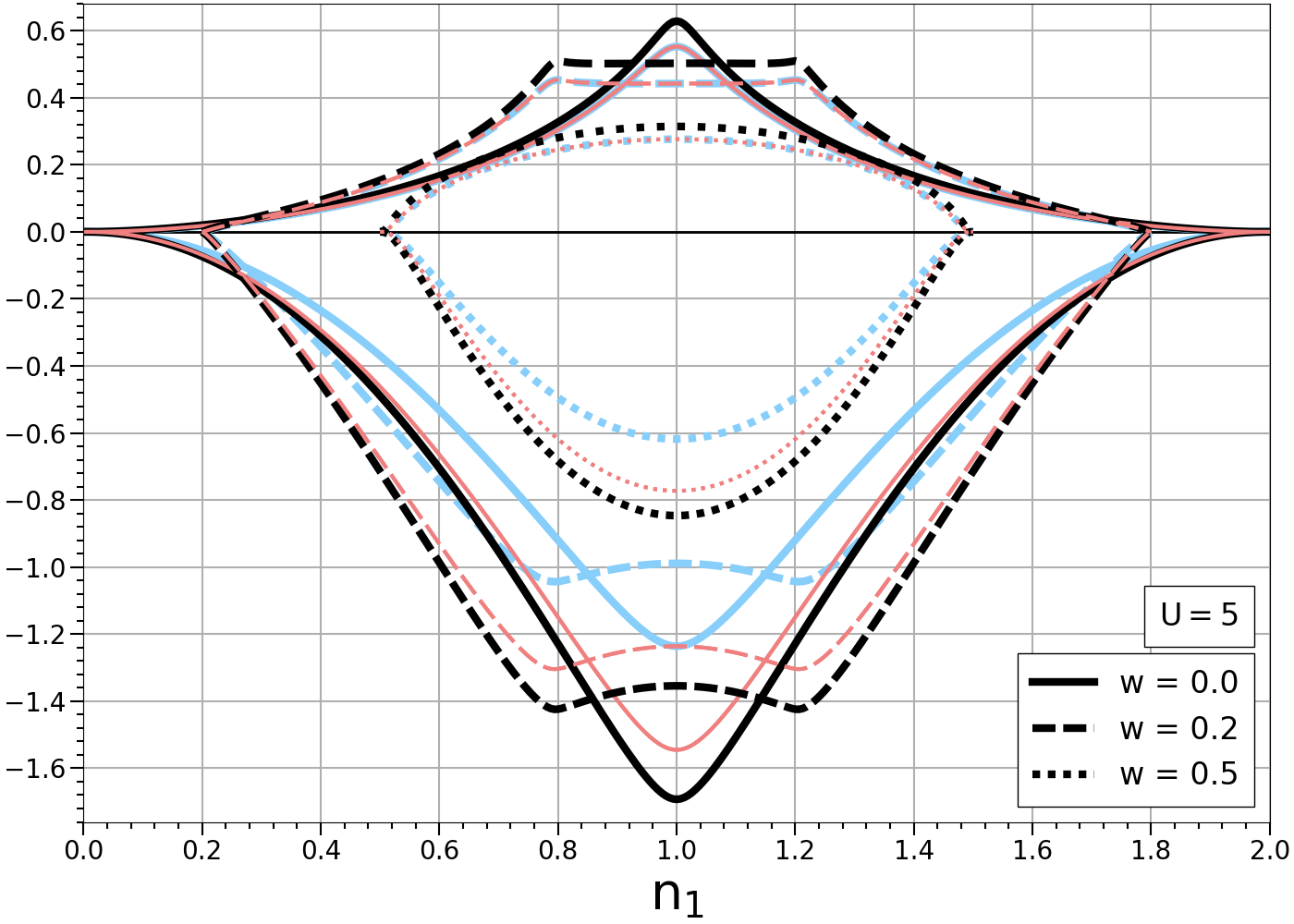
Figure 1: The Hubbard dimer singlet bi-ensemble correlation energies (negative values) and kinetic contribution (positive values) for $U=4$ (light blue) and $U=5$ (black) as a function of site-occupation and different weights. Red curves deduced from $U=4$ constrain the $U=5$ curve via Eq. 21.

EDFT is a formally exact generalization of ground-state KS-DFT, where the ensemble consists of several eigenstates of an $N$-electron system. Consider any ensemble density matrix, ${\hat{\Gamma}}_{w}$, of the form

$${\hat{\Gamma}}_{w}({\bf r}_{1}...{\bf r}_{N},{\bf r}^{\prime}_{1}...{\bf r}^{\prime}_{N})=\sum_{m=0}^{M}w_{m}\ket{\Psi_{m}({\bf r}_{1}...{\bf r}_{N})}\bra{\Psi_{m}({\bf r}^{\prime}_{1}...{\bf r}^{\prime}_{N})},$$ (1)

where $\Psi_{m}$ are any orthonormal wave functions, and $w_{m}$ are positive monotonically non-increasing weights that are normalized. The expectation value of any operator $\hat{A}$ is then

$$A[{\hat{\Gamma}}_{w}]=\text{Tr}\{{\hat{\Gamma}}_{w}\hat{A}\}=\sum_{m=0}^{M}w_{m}\bra{\Psi_{m}}\hat{A}\ket{\Psi_{m}}.$$ (2)

An ensemble energy is then the variational minimum of the Hamiltonian, yielding

$$E_{w}=\min_{\Gamma_{w}}\text{Tr}\{{\hat{\Gamma}}_{w}{\hat{H}}\},$$ (3)

where $m$ labels the eigenstates, in order of increasing energy, and $E_{m}$ are the eigenvalues. Transition energies can be deduced from differences between ensemble calculations of differing weights. Oliveira et al. (1988) EDFT tells us that there exists a $w$-dependent density functional

$$F_{w}[n]=\min_{\Gamma_{w}\rightarrow n}\text{Tr}\{{\hat{\Gamma}}_{w}({\hat{T}}+{\hat{V}}_{\rm ee})\},$$ (4)

where ${\hat{T}}$ is the kinetic energy operator and ${\hat{V}}_{\rm ee}$ is the electron-electron repulsion. We denote the minimizer by $\Gamma_{w}[n]$. Then

$$E_{w}=\min_{n}\left\{F_{w}[n]+\int n({\bf r})v({\bf r})d{\bf r}\right\},$$ (5)

where $v({\bf r})$ is the external potential. Any expectation value can be converted into a density functional via $A[n]=A[\Gamma_{w}[n]]$ . The minimizing density is

$$n_{w}({\bf r})=\sum_{m=0}^{M}w_{m}n_{m}({\bf r}),$$ (6)

where $n_{m}({\bf r})$ is the density of the $m$-th level.

A key facet of EDFT is that the equivalence between the exact density and the non-interacting KS density is only true for the ensemble average, and it is not necessarily true for the individual densities within the weighted sum. The following conditions are true only for the ensemble energy, not the individual excited-state energies.

Uniform coordinate scaling has been responsible for multiple advances in DFT. However, coordinate scaling investigations in EDFT have thus far only been used to define the adiabatic connection formula for the exchange-correlation energy Nagy (1995) or examining the behavior of EDFT in the low-density and high-density regimes, without formal theorems based on scaling. Gould et al. (2023) Additional work on foundational theorems include the virial theorem for EDFT by Nagy Nagy (2013, 2002, 2011) and the signs of correlation energy components, by Pribram-Jones et al. Pribram-Jones et al. (2014) We build on this foundation by deriving uniform scaling inequalities based on the variational definition of the ensemble functional. Levy and Perdew (1985); Pittalis et al. (2011) We also provide numerical verification and proofs of the basic principles and some additional exact conditions.

We use norm-preserving homogeneous scaling of the coordinate r$\rightarrow\gamma{\bf r}$ with $0<\gamma<\infty$. The scaled density matrix is defined as

$$\Gamma_{w,\gamma}({\bf r}_{1}...{\bf r}^{\prime}_{N}):=\gamma^{3N}\,\Gamma_{w}(\gamma{\bf r}_{1}...\gamma{\bf r}^{\prime}_{N}),$$ (7)

and a scaled density is $n_{\gamma}({\bf r})=\gamma^{3}n(\gamma{\bf r})$. Trivially,

$$T[\Gamma_{w,\gamma}]=\gamma^{2}T[\Gamma_{w}],~{}~{}~{}V_{\rm ee}[\Gamma_{w,\gamma}]=\gamma\,V_{\rm ee}[\Gamma_{w}].$$ (8)

Because these scale differently, $\Gamma_{w,\gamma}[n]\neq\Gamma_{w}[n_{\gamma}]$. By the variational principle, $F[n_{w,\gamma}]\leq F[{\hat{\Gamma}}_{w,\gamma}[n]]$, which gives the fundamental inequality of scaling,

$$T_{w}[n_{\gamma}]+V_{{\rm ee},w}[n_{\gamma}]\leq\gamma^{2}T_{w}[n]+\gamma V_{{\rm ee},w}[n].$$ (9)

Manipulation of this formula yields, for $\gamma\geq 1$, Levy and Perdew (1985)

$$T_{w}[n_{\gamma}]\leq\gamma^{2}T_{w}[n],~{}~{}~{}~{}V_{{\rm ee},w}[n_{\gamma}]\geq\gamma V_{{\rm ee},w}[n],~{}~{}~{}~{}\gamma\geq 1$$ (10)

and setting $\gamma\rightarrow 1/\gamma$ yields results for $\gamma\leq 1$.

Next, we turn to the KS scheme, used in modern EDFT approaches. Here $F_{w}[n]=T_{{\scriptscriptstyle\rm S},w}[n]+E_{{\scriptscriptstyle\rm HXC},w}[n]$ where $T_{{\scriptscriptstyle\rm S},w}$ is the KS kinetic energy and $E_{{\scriptscriptstyle\rm HXC},w}$ is the Hartree-exchange-correlation. Because there is no interaction,

$$T_{{\scriptscriptstyle\rm S},w}[n_{\gamma}]=\gamma^{2}T_{{\scriptscriptstyle\rm S},w}[n].$$ (11)

Moreover, because the Hartree-exchange is linear in the scaling parameter:

$$E_{{\scriptscriptstyle\rm HX},w}[n_{\gamma}]=\gamma E_{{\scriptscriptstyle\rm HX},w}[n].$$ (12)

In EDFT, separation of Hartree from exchange is more complicated than in ground-state DFT. Gould et al. (2023); Yang (2021); Gould and Pittalis (2019) Subtracting these larger energies following the usual procedure from ground-state DFT Levy and Perdew (1985) yields, for $\gamma\geq 1$,

$$T_{{\scriptscriptstyle\rm C},w}[n_{\gamma}]\leq\gamma^{2}T_{{\scriptscriptstyle\rm C},w}[n],~{}~{}~{}~{}E_{{\scriptscriptstyle\rm C},w}[n_{\gamma}]\geq\gamma E_{{\scriptscriptstyle\rm C},w}[n],~{}~{}~{}\gamma\geq 1$$ (13)

where $E_{{\scriptscriptstyle\rm C},w}[n]$ is the correlation energy, and $T_{{\scriptscriptstyle\rm C},w}=T_{w}-T_{{\scriptscriptstyle\rm S},w}$ is its kinetic contribution. Considering $\gamma=1+\epsilon$ in Eq.13, and taking $\epsilon\rightarrow 0$, yields differential versions of Eq. 13:

$$\frac{d}{d\gamma}\left\{\frac{T_{{\scriptscriptstyle\rm C},w}[n_{\gamma}]}{\gamma^{2}}\right\}\leq 0,~{}~{}~{}~{}\frac{d}{d\gamma}\left\{\frac{E_{{\scriptscriptstyle\rm C},w}[n_{\gamma}]}{\gamma}\right\}\geq 0$$ (14)

Combining these using Nagy’s generalization (Eq. 24 of Ref. 44) of the ground-state equality

$$\left.\frac{dE_{{\scriptscriptstyle\rm C},w}[n_{\gamma}]}{d\gamma}\right|_{\gamma=1}=E_{{\scriptscriptstyle\rm C},w}[n]+T_{{\scriptscriptstyle\rm C},w}[n],$$ (15)

we find

$$\bigg{(}2-2\gamma\frac{d}{d\gamma}+\gamma^{2}\frac{d^{2}}{d\gamma^{2}}\bigg{)}\,E_{{\scriptscriptstyle\rm C},w}[n_{\gamma}]\leq 0,$$ (16)

the condition for concavity in the ensemble correlation energy. This is the ensemble form of Eq. 40 in Ref. 47. Eqs. 9, 13, and 16 are primary results of the current work, being the ensemble generalizations of their ground-state analogs.

An immediate application of Eq. 12 is to extract the HX component from any HXC approximation. As the conditions limit growth with $\gamma$,

$$E_{{\scriptscriptstyle\rm HX},w}[n]=\lim_{\gamma\rightarrow\infty}E_{{\scriptscriptstyle\rm HXC},w}[n_{\gamma}]/\gamma,$$ (17)

an exact condition which can prove useful for separating HX from C components. Gould and Pittalis (2017); Gould et al. (2023)

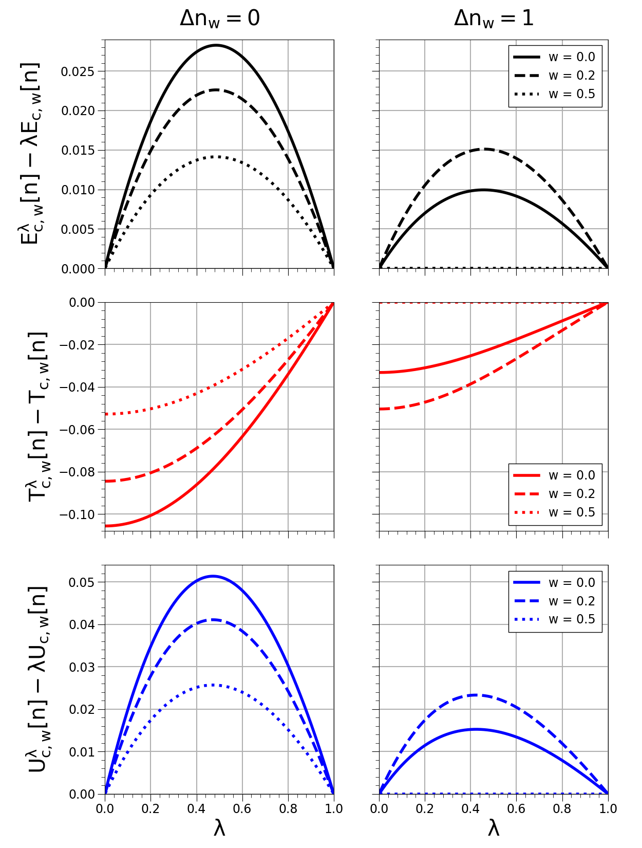
Figure 2: Correlation inequalities (Eq. 21) for the total (top), kinetic (middle), and potential (bottom) correlation energies, depicted by varying $\lambda$ in the Hubbard dimer bi-ensemble with $U=1$. More cases are provided in Figs. S6-S7 of the supplemental material.

To conclude this section, we use the pioneering relationship between coupling constant and coordinate scaling. Defining $\lambda$ dependence via

$$F^{\lambda}_{w}[n]=\min_{\Gamma_{w}\rightarrow n}\text{Tr}\{\Gamma_{w}({\hat{T}}+\lambda{\hat{V}}_{\rm ee})\},$$ (18)

Nagy showed Nagy (1995)

$$E_{{\scriptscriptstyle\rm HXC},w}^{\lambda}[n]=\lambda^{2}E_{{\scriptscriptstyle\rm HXC},w}[n_{1/\lambda}].$$ (19)

Using Eq. 19, it is possible to rewrite all results given in terms of scaled densities as $\lambda$-dependent relations. Such relations are well known and much used in ground-state DFT, via the adiabatic connection formalism. Harris (1984); Ernzerhof (1996) For real-space Hamiltonians, these relations are simply a rewriting of the scaling relations in a more popular form, but they also apply to lattice Hamiltonians, where scaling is not possible. Converting from scaling in Eq. 15 gives

$$T^{\lambda}_{{\scriptscriptstyle\rm C},w}[n]=E^{\lambda}_{{\scriptscriptstyle\rm C},w}[n]-\lambda\frac{dE^{\lambda}_{{\scriptscriptstyle\rm C},w}[n]}{d\lambda}.$$ (20)

The scaling inequalities (Eqs. 13) become

$$T_{{\scriptscriptstyle\rm C},w}^{\lambda}[n]\leq T_{{\scriptscriptstyle\rm C},w}[n],~{}~{}~{}E_{{\scriptscriptstyle\rm C},w}^{\lambda}[n]\geq\lambda E_{{\scriptscriptstyle\rm C},w}[n],~{}~{}~{}~{}\lambda\leq 1,$$ (21)

with differential versions

$$\frac{dT_{{\scriptscriptstyle\rm C},w}^{\lambda}[n]}{d\lambda}\leq 0,~{}~{}~{}E_{{\scriptscriptstyle\rm C},w}^{\lambda}[n]\geq\lambda\,\frac{dE_{{\scriptscriptstyle\rm C},w}^{\lambda}[n]}{d\lambda},$$ (22)

while Eq.  16 becomes quite simply:

$$\frac{d^{2}E_{{\scriptscriptstyle\rm C},w}^{\lambda}[n]}{d\lambda^{2}}\leq 0.$$ (23)

Note that all inequalities for $E_{{\scriptscriptstyle\rm C},w}$, both coordinate-scaled (Eqs. 13, 14) and $\lambda$-dependent (Eqs. 21, 22), are also true for $U_{{\scriptscriptstyle\rm C},w}=E_{{\scriptscriptstyle\rm C},w}-T_{{\scriptscriptstyle\rm C},w}$, the potential contribution to correlation. The HX energy (Eq. 17) may be extracted via

$$E_{{\scriptscriptstyle\rm HX},w}[n]=\lim_{\lambda\rightarrow 0}E^{\lambda}_{{\scriptscriptstyle\rm HXC},w}[n]/\lambda.$$ (24)

Our last condition concerns the relationship between DFT and traditional approaches to quantum chemistry. In the ground state, it has long been known Crisostomo et al. (2022); Löwdin (1955) that $0\geq E_{\scriptscriptstyle\rm C}^{\rm HF}\geq E_{\scriptscriptstyle\rm C}$, where $E_{\scriptscriptstyle\rm C}^{\rm HF}$ is the traditional definition of the correlation energy, i.e., relative to the Hartree-Fock (HF) energy (we treat only restricted HF here, RHF). Given the complications of EDFT, we discuss here only the case of the first singlet bi-ensemble for two electrons. In this case, we equate EHF with an EDFT EXX calculation (’exact exchange only’). The only difference between EHF and EDFT is that the EHF quantities are evaluated on the approximate EHF density, while EDFT quantities are evaluated on the exact density. Exactly the same variational reasoning leads us to

$$0\geq E_{{\scriptscriptstyle\rm C},w}^{\rm HF}\geq E_{{\scriptscriptstyle\rm C},w}[n]$$ (25)

where $E_{{\scriptscriptstyle\rm C},w}^{\rm HF}=E_{w}-E_{w}^{\rm HF}$, and $E_{w}^{\rm HF}$ minimizes $F_{w}=T_{{\scriptscriptstyle\rm S},w}+E_{{\scriptscriptstyle\rm HX},w}$. We leave the more general case to braver souls.

Figure 3: Ensemble adiabatic connection with $\Delta n_{w}=0$ and $U=5$; circles represent the weight-dependent HX energy, which the HXC expression approaches as $\lambda\to 0$ (Eq. 24). More cases are provided in Fig. S8 of the supplemental material.

The Hamiltonian of the Hubbard dimer is

$${\hat{H}}=-t\sum_{\sigma}(\hat{c}^{\dagger}_{1\sigma}\hat{c}_{2\sigma}+h.c.)+U\sum_{i}\hat{n}_{i\uparrow}\hat{n}_{i\downarrow}+\sum_{i}v_{i}\hat{n}_{i},\\$$ (26)

where $t$ is the hopping parameter, $U$ the on-site electrostatic self-repulsion, and $v_{i}$ the on-site potential (which controls the asymmetry of the dimer). For this lattice system, with $N=2$, the electronic density is characterized by a single number, the difference between occupations of the two sites, $\Delta n=n_{2}-n_{1}$. The $\lambda$-dependence of any quantity is found by replacing $U$ by $\lambda U$, keeping $\Delta n$ fixed. We choose $t=1/2$ everywhere.

We consider the simplest bi-ensemble, a mixture of the ground-state with the first excited singlet. Full analytic expressions of $\ket{\Psi_{0}}$ and $\ket{\Psi_{1}}$, as well as plots of various bi-ensemble quantities, are given in the supplemental material in section 1. The value of $\Delta n_{w}$ is constrained by $w$:

$$|\Delta n_{w}|\leq 2\overline{w},$$ (27)

where $\overline{w}=1-w$, i.e. is smaller than that of the ground state ($w=0$). Densities are shown in Fig. S1 of the supplemental material. The total energy of the ensemble is defined as

$$E_{w}=\overline{w}\bra{\Psi_{0}}\hat{H}\ket{\Psi_{0}}+w\bra{\Psi_{1}}\hat{H}\ket{\Psi_{1}}.$$ (28)

Plots of $E_{w}$ are depicted in Figs. S2-S3 of the supplemental material, showing the quantity both as a function of $\Delta v$ and $\Delta n_{w}$. We also show analogous plots of $F_{w}=E_{w}-\Delta v\Delta n_{w}/2$ in Figs. S4-S5. For this bi-ensemble, the exact HX energy has the simple analytical form Deur et al. (2017):

$$E_{{\scriptscriptstyle\rm HX},w}=\frac{U}{2}\left[1+w+\frac{(1-3w)}{\overline{w}^{2}}\frac{\Delta n_{w}^{2}}{4}\right].$$ (29)

Inequalitites. We plot $\lambda$-dependencies in Fig. 2 that have a definite sign according to Eq. 13. We show several values of $w$ for two densities for $U=1$ (moderate correlation). Scanning over all $U$ and $\Delta n_{w}$, these inequalities are always satisfied. For the symmetric dimer ($\Delta n_{w}=0$), $w=0.0$ has the largest maximum and $w=0.5$ has the smallest. As $\Delta n_{w}$ is increased, the trend disappears and the curves are not monotonic in $w$. For $w=0.5$, the inequality becomes an equality for $\Delta n_{w}=1$, the maximum representable value of $\Delta n$ for the ensemble. In Fig. 3, we show that all $U_{{\scriptscriptstyle\rm HXC},w}$ curves approach their corresponding HX value as $\lambda\rightarrow 0$, in accordance with Eq. 24. More plots of Figs. 2 and 3 for various combinations of $w$ and $\Delta n_{w}$ are provided in Figs. S6-S8 of the supplemental material.

The non-monotonic behavior in Fig. 1 can be easily understood. By definition, $E_{w}(\Delta v)$ is linear in $w$, as is $F_{w}$. But, when converted to density functionals, and with KS quantities subtracted, these become highly non-monotonic, as shown in Figs. S2 and S3 in the supplemental material.

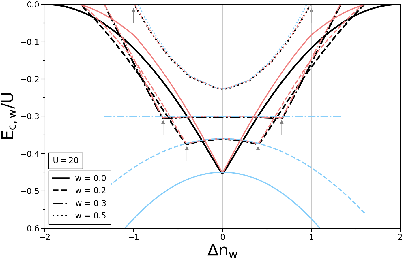
Figure 4: Exact correlation energy (black), leading-order expansion in large $U$ (red) and the expansion in the symmetric limit (blue) for the correlation energy are all plotted as a function of the exact density. Small arrows indicate the region between $2w$ and $-2w$ where the symmetric expansion matches the exact.

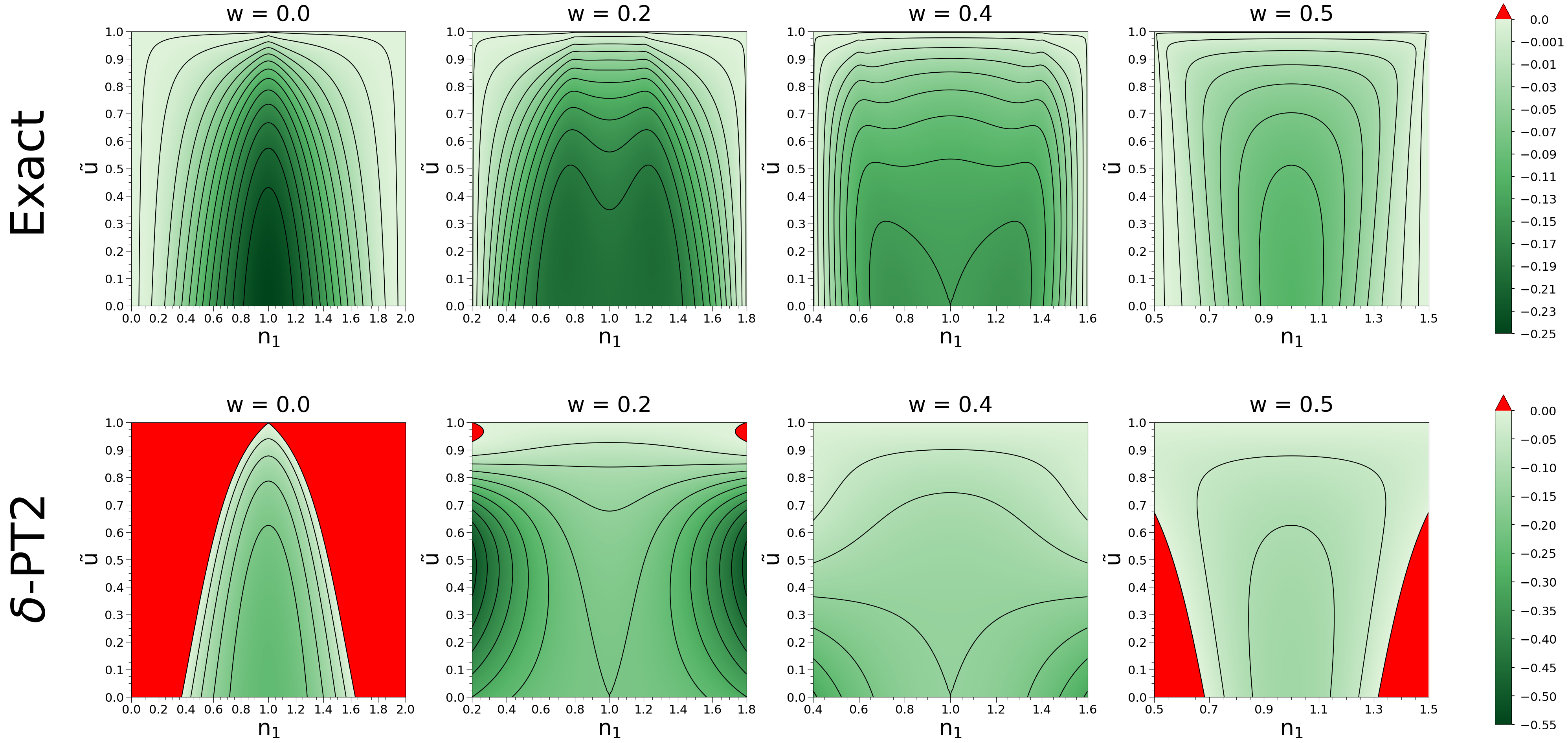
Figure 5: The second derivative of the Hubbard dimer bi-ensemble correlation energy with respect to $U$ for all values of the reduced variable $\tilde{u}=U/\sqrt{1+U^{2}}$. The concavity condition is satisfied, but is violated by the $\delta$-PT2 approximation in certain regimes (red denotes positive). But $U$-PT2 automatically satisfies it, by construction.

Strong Correlation. In Fig. 4 we plot the exact correlation energy, our approximation (Eq. S.16 of the supplemental material), and the symmetric limit expansion of Deur et al. Deur et al. (2018), each evaluated at the exact density. The last yields the strongly correlated correlation energy only for $|\Delta n_{w}|\leq 2w$, but our expansion yields the correct limit for all allowed $\Delta n_{w}$, including the slope discontinuity at $|\Delta n_{w}|=2w$. Such $w$-dependent derivative discontinuities occur only in EDFT. The approximate weight-dependent strongly correlated correlation energy is derived in the supplemental material along with further analysis of the energy components and approximation of the density. For the strong-interaction limit of the dimer, the correlation energy contains a non-trivial weight-dependence. This differs from real space Gould et al. (2023) where the energies were found to be weight-independent. This is not a counter example, because the dimer is a site-model. This difference manifests in the expansion of the strongly correlated energies in powers of the coupling-constant. Our first correction, relative to the leading term, is $\mathcal{O}(\lambda^{-2})$ and differs qualitatively from the $\mathcal{O}(\lambda^{-1/2})$ behavior found by Gould and coauthors.

Concavity Condition of the Correlation Energy. We illustrate the concavity condition of Eq. 23 using contour plots depicting all possible combinations of $U$ and $n_{1}$, making use of the reduced variable $\tilde{u}=U/\sqrt{1+U^{2}}$. Illustrated by Fig. 5, the second derivative is negative for all values of $U$ and thus satisfies the concavity condition for all electronic correlation strengths.

The standard use of exact conditions in DFT is to ensure that approximate functionals satisfy them. Pederson and Burke (2023) We illustrate our conditions by applying them to existing approximations on the Hubbard model. The first is the standard many-body expansion in powers of the interaction, $U$, which we perform up to 2nd-order, i.e., the analog of Møller-Plesset perturbation theory, denoted $U$-PT2. The second is less familiar: an expansion in powers of $\Delta n$ around the symmetric case, $\Delta n=0$, called $\delta$-PT2. Deur et al. (2018) This can be considered a (tortured) analog of the gradient expansion of DFT, Perdew et al. (1996) as it is an expansion around the uniform limit. Fig. 5 shows that the $\delta$-PT2 approximation violates the concavity condition, even for $w=0$, while $U$-PT2 never does. The violations are not monotonic with increasing weights, as $w=0.4$ has none. Deur et al. reported that, compared to U-PT2, $\delta$-PT2 produced more accurate equi-ensemble energies and densities. Likely, the accuracy of $\delta$-PT2 could be further improved by imposing concavity. Recent advances in EDFT, such as the direct ensemble correction Yang et al. (2017) and the perturbative EDFT method, Gould et al. (2022) are explicitly computed in the perturbative limit, $w\rightarrow 0^{+}$. If an approximation is derived before such a limit is taken, and its ground-state approximation satisfies concavity; the resulting approximation should satisfy concavity also.

Quantum Chemistry. Finally, we examine in detail the difference between the DFT and HF correlation energies and their components in Figs. S5, S6, and S7 in the supplemental material. We provide plots of the exact/EHF total correlation energies for the dimer bi-ensemble, where we show the ground-state inequalities ($E^{\rm HF}_{\scriptscriptstyle\rm C}\geq E_{\scriptscriptstyle\rm C}$) holds for any $w$-value (Figs. S3 and S4). It also is known that $T_{\scriptscriptstyle\rm C}^{\rm HF}$ can become negative in the ground state of the Hubbard dimer, Giarrusso and Pribram-Jones (2022) and we find this is also true when $w\neq 0$, but this is likely an artifact of lattice Hamiltonians that cannot occur in the real-space analog.Crisostomo et al. (2023, 2022)

This work provides new exact conditions for EDFT which can be used to analyze and/or improve new approximations in EDFT. Further work is being performed to improve approximations and provide a pathway to accurate EDFT functionals.

In the supplemental material for this article we provide analytical expressions (and plots) for various weight-dependent quantities of interest for the Hubbard dimer bi-ensemble, giving both the exact/EHF solution.

T.R.S. thanks the Molecular Software Science Institute for funding, award no. 480718-19905B, and Sina Mostafanejad for fruitful discussions. K.B., J.K., and S.C. acknowledge support from NSF award number CHE-2154371. A.P.J. acknowledges financial support for this publication from Cottrell Scholar Award #28281, sponsored by Research Corporation for Science Advancement.

References

- Hohenberg and Kohn (1964) P. Hohenberg and W. Kohn, Phys. Rev. 136, B864 (1964).
- Kohn and Sham (1965) W. Kohn and L. J. Sham, Phys. Rev. 140, A1133 (1965).
- Burke (2012) K. Burke, J. Chem. Phys. 136, 150901 (2012).
- Becke (2014) A. D. Becke, J. Chem. Phys. 140, 18A301 (2014).
- Jones (2015) R. O. Jones, Rev. Mod. Phys. 87, 897 (2015).
- Morgante and Peverati (2020) P. Morgante and R. Peverati, Int. J. Quantum. Chem. 120, e26332 (2020).
- Ullrich (2011) C. A. Ullrich, Time-dependent density-functional theory: concepts and applications (OUP Oxford, 2011).
- Runge and Gross (1984) E. Runge and E. K. Gross, Phys. Rev. Lett. 52, 997 (1984).
- Casida (1996) M. Casida, Time-dependent density functional response theory of molecular systems: Theory, computational methods, and functionals (Elsevier, 1996), vol. 4.
- Marques et al. (2012) M. A. Marques, N. T. Maitra, F. M. Nogueira, E. K. Gross, and A. Rubio, Fundamentals of time-dependent density functional theory, vol. 837 (Springer, 2012).
- Maitra (2016) N. T. Maitra, J. Chem. Phys. 144, 220901 (2016).
- Tozer (2003) D. J. Tozer, J. Chem. Phys. 119, 12697 (2003).
- Levine et al. (2006) B. G. Levine, C. Ko, J. Quenneville, and T. J. MartÍnez, Mol. Phys. 104, 1039 (2006).
- Huix-Rotllant et al. (2011) M. Huix-Rotllant, A. Ipatov, A. Rubio, and M. E. Casida, Chem. Phys. 391, 120 (2011).
- Theophilou (1979) A. K. Theophilou, J. Phys. C: Solid State Phys. 12, 5419 (1979).
- Gross et al. (1988a) E. K. Gross, L. N. Oliveira, and W. Kohn, Phys. Rev. A 37, 2805 (1988a).
- Gross et al. (1988b) E. K. Gross, L. N. Oliveira, and W. Kohn, Phys. Rev. A 37, 2809 (1988b).
- Yang et al. (2014) Z.-h. Yang, J. R. Trail, A. Pribram-Jones, K. Burke, R. J. Needs, and C. A. Ullrich, Phys. Rev. A 90, 042501 (2014).
- Pribram-Jones et al. (2014) A. Pribram-Jones, Z.-h. Yang, J. R. Trail, K. Burke, R. J. Needs, and C. A. Ullrich, J. Chem. Phys. 140, 18A541 (2014).
- Yang et al. (2017) Z.-h. Yang, A. Pribram-Jones, K. Burke, and C. A. Ullrich, Phys. Rev. Lett. 119, 033003 (2017).
- Gould and Pittalis (2017) T. Gould and S. Pittalis, Phys. Rev. Lett. 119, 243001 (2017).
- Deur and Fromager (2019) K. Deur and E. Fromager, J. Chem. Phys. 150, 094106 (2019).
- Deur et al. (2017) K. Deur, L. Mazouin, and E. Fromager, Phys. Rev. B 95, 035120 (2017).
- Gould and Pittalis (2019) T. Gould and S. Pittalis, Phys. Rev. Lett. 123, 016401 (2019).
- Fromager (2020) E. Fromager, Phys. Rev. Lett. 124, 243001 (2020).
- Gould and Pittalis (2020) T. Gould and S. Pittalis, Aust. J. Chem. 73, 714 (2020).
- Gould et al. (2020) T. Gould, G. Stefanucci, and S. Pittalis, Phys. Rev. Lett. 125, 233001 (2020).
- Gould and Kronik (2021) T. Gould and L. Kronik, J. Chem. Phys. 154, 094125 (2021).
- Gould (2020) T. Gould, J. Phys. Chem. Lett. 11, 9907 (2020).
- Loos and Fromager (2020) P.-F. Loos and E. Fromager, J. Chem. Phys. 152, 214101 (2020).
- Marut et al. (2020) C. Marut, B. Senjean, E. Fromager, and P.-F. Loos, Faraday Discuss. 224, 402 (2020).
- Gould et al. (2021) T. Gould, L. Kronik, and S. Pittalis, Phys. Rev. A 104, 022803 (2021).
- Yang (2021) Z.-h. Yang, Phys. Rev. A 104, 052806 (2021).
- Cernatic et al. (2022) F. Cernatic, B. Senjean, V. Robert, and E. Fromager, Top. Curr. Chem. 380, 1 (2022).
- Sagredo and Burke (2018) F. Sagredo and K. Burke, J. Chem. Phys. 149, 134103 (2018).
- Perdew et al. (1996) J. P. Perdew, K. Burke, and M. Ernzerhof, Phys. Rev. Lett. 77, 3865 (1996).
- Levy and Perdew (1985) M. Levy and J. P. Perdew, Phys. Rev. A 32, 2010 (1985).
- Pederson and Burke (2023) R. Pederson and K. Burke, arXiv preprint arXiv:2303.01766 (2023).
- Hubbard (1963) J. Hubbard, Proc. R. Soc. Lond. USA A 276, 238 (1963).
- Oliveira et al. (1988) L. N. d. Oliveira, E. Gross, and W. Kohn, Phys. Rev. A 37, 2821 (1988).
- Nagy (1995) Á. Nagy, Int. J. Quantum Chem. 56, 225 (1995).
- Gould et al. (2023) T. Gould, D. P. Kooi, P. Gori-Giorgi, and S. Pittalis, Phys. Rev. Lett. 130, 106401 (2023).
- Nagy (2013) Á. Nagy, Local virial theorem for ensembles of excited states (CRC Press, 2013), p. 135.
- Nagy (2002) Á. Nagy, in Recent Advances In Density Functional Methods: Part III (World Scientific, 2002), pp. 247–256.
- Nagy (2011) A. Nagy, J. Chem. Phys. 135, 044106 (2011).
- Pittalis et al. (2011) S. Pittalis, C. Proetto, A. Floris, A. Sanna, C. Bersier, K. Burke, and E. K. Gross, Phys. Rev. Lett. 107, 163001 (2011).
- Levy and Perdew (1993) M. Levy and J. P. Perdew, Phys. Rev. B 48, 11638 (1993).
- Harris (1984) J. Harris, Phys. Rev. A 29, 1648 (1984).
- Ernzerhof (1996) M. Ernzerhof, Chem. Phys. Lett. 263, 499 (1996).
- Crisostomo et al. (2022) S. Crisostomo, M. Levy, and K. Burke, J. Chem. Phys. 157, 154106 (2022).
- Löwdin (1955) P.-O. Löwdin, Phys. Rev. 97, 1509 (1955).
- Deur et al. (2018) K. Deur, L. Mazouin, B. Senjean, and E. Fromager, The European Physical Journal B 91, 1 (2018).
- Gould et al. (2022) T. Gould, Z. Hashimi, L. Kronik, and S. G. Dale, J. Phys. Chem. Lett. 13, 2452 (2022).
- Giarrusso and Pribram-Jones (2022) S. Giarrusso and A. Pribram-Jones, J. Chem. Phys. 157, 054102 (2022).
- Crisostomo et al. (2023) S. Crisostomo, R. Pederson, J. Kozlowski, B. Kalita, A. C. Cancio, K. Datchev, A. Wasserman, S. Song, and K. Burke, Lett. Math Phys. 113, 42 (2023).