An Interpretable Constructive Algorithm for Incremental Random Weight Neural Networks and Its Application

Abstract

Incremental random weight neural networks (IRWNNs) have gained attention in view of its easy implementation and fast learning. However, a significant drawback of IRWNNs is that the relationship between the hidden parameters (node) and the residual error (model performance) is difficult to be interpreted. To address the above issue, this article proposes an interpretable constructive algorithm (ICA) with geometric information constraint. First, based on the geometric relationship between the hidden parameters and the residual error, an interpretable geometric information constraint is proposed to randomly assign the hidden parameters. Meanwhile, a node pool strategy is employed to obtain hidden parameters that is more conducive to convergence from hidden parameters satisfying the proposed constraint. Furthermore, the universal approximation property of the ICA is proved. Finally, a lightweight version of ICA is presented for large-scale data modeling tasks. Experimental results on six benchmark datasets and a numerical simulation dataset demonstrate that the ICA outperforms other constructive algorithms in terms of modeling speed, model accuracy, and model network structure. Besides, two practical industrial application case are used to validate the effectiveness of ICA in practical applications.

I Introduction

Neural networks (NNs), a promising computing paradigm that thoroughly differs from traditional model-based computing, can learn amazingly well patterns from complex data. Therefore, it should not be surprising that NNs are applied in a variety of research fields[1, 2, 3]. The most popular NNs are the deep neural networks (DNNs) and the flat neural networks (FNNs). DNNs realize end-to-end learning by organically combining unsupervised layer-by-layer pre-training with supervised fine-tuning[4]. This learning approach makes DNNs have great potential in expressive power and generalization ability, but it also leads to a time-consuming training process. Recently, due to the universal approximation ability, RWNNs, as a typical representative of FNNs, have been receiving increasing interset[5, 6, 7, 8]. RWNNs are characterized by a two-step training paradigm, i.e., randomly assigning the hidden parameters, and evaluating the output weights by solving a system of linear equations.

Despite the aforementioned advantages, little is known about how network structure for RWNNs fits into modeling tasks. Too large a network structure will result in a poor generalization, while too small a network structure will cause insufficient learning ability. The constructive algorithms always begin with a small network structure (usually a hidden node) and dynamically grow the network structure by adding new hidden nodes incrementally until the requirements are met[9]. This means that the constructive algorithms are likely to offer smaller network structure for modeling tasks[10]. Therefore, constructive version of RWNNs (incremental RWNNs, IRWNNs) have been successfully applied for data modeling tasks[11, 12, 13].

From the perspective of probability theory, the randomly generated hidden parameters are not necessarily suitable for IRWNNs. Therefore, a natural question arises: What hidden parameters are good for IRWNNs? Based on algebraic study of multidimensional nonlinear functions, [14] proved that the relationship between input samples and hidden parameters can be expressed by nonlinear weight equations. [15] showed that there exists a supervisory mechanism between the hidden parameters and the input samples for better network performance. [16] proposed a constructive algorithm with supervisory mechanism to randomly assign hidden parameters in the dynamical interval. [17] proposed a hidden parameters generation approach by analyzing the input samples scope and activation function. Recently, [18] proposed RWNNs with compact incremental inequality constraints, i.e., CIRWN, to improve the quality of hidden parameters. Although these approaches further improve the potential of IRWNNs, very little is known about how hidden parameters accomplish their goals. That is, it is difficult to visualize the influence of each hidden parameter on residual error (network performance). At present, how to interpret the predicted behavior of NNs to improve interpretability is a meaningful and important topic[19, 20]. Thus, further research on interpretable constructive algorithm is important and necessary for RWNNs.

Motivated by the above analysis, this paper proposes an interpretable constructive algorithm (ICA) to help people understand the nature behind the predicted behavior of RWNNs. The main contributions are listed below:

1) The geometric relationship between the hidden parameters and the residual error is employed to build an interpretable geometric information constraint for assigning the randomized hidden parameters in the incremental construction process, and the theoretical analysis is fully discussed.

2) A node pool strategy is developed to further improve the quality of the hidden nodes by searching the hidden parameters that are more conducive to convergence.

3) Using different calculation methods of network output weights, two algorithm implementations, namely ICA and ICA+, are proposed.

The remainder of the article is organized as follows. Section 2 briefly reviews RWNNs and the constructive algorithms. Section 3 proposes an interpretable constructive algorithm and describes it in detail. In section 4, a numerical simulation dataset, six real-world datasets, an ore grinding semi-physical simulation platform, and a gesture recognition system are considered to evaluate the effectiveness and efficiency of the proposed ICA and ICA+. Finally, conclusions are drawn in section 5.

II Preliminaries

II-A Random Weight Neural Networks

RWNNs can be regarded as a flatted network, where all the hidden parameters (the input weights and biases) are randomly assigned from a fixed interval and fixed during the training process. The output weights are evaluated by solving a system of linear equations. The theory of RWNNs is described as follows.

For a target function $f:{R^{d}}\to{R^{m}}$, the RWNNs with $L$ hidden nodes can be written as : ${f_{L}}=H\beta$, where $H=\left[{{g_{1}}\left({\omega_{1}^{\rm{T}}\cdot x+{b_{1}}}\right),\cdots,{g_{L}}\left({\omega_{L}^{\rm{T}}\cdot x+{b_{L}}}\right)}\right]$, T denotes matrix transpose, $x$ is the input sample, ${\omega_{j}}$ and ${b_{j}}$ are the input weights and biases of the $j$-th hidden node, respectively. $j=1,\cdots,L$, ${g_{j}}$ denotes the nonlinear activation function of the $j$-th hidden node. The output weights ${\beta}$ are evaluated by $\beta={H^{\dagger}}{f_{L}}$, where $\beta=\left[{{\beta_{1}},{\beta_{2}},...,{\beta_{L}}}\right]^{\rm{T}}$, ${H^{\dagger}}$ denotes the Moore-Penrose generalized inverse of $H$.

II-B Constructive Algorithms

Constructive algorithms are likely to find the minimal network structure due to their incremental construction nature. Therefore, the constructive algorithms are introduced RWWNs, namely IRWNNs. Specifically, assuming that the IRWNNs with $L-1$ hidden nodes does not reach the termination condition, then a new hidden node will be generated by the following two steps:

1) The input weights ${\omega_{L}}$ and bias ${b_{L}}$ are randomly generated from the fixed interval ${\left[{-\lambda,\lambda}\right]^{d}}$ and $\left[{-\lambda,\lambda}\right]$. In particular, $\lambda$ usually takes the value 1. Then, the output vector ${g_{L}}$ of the $L$-th hidden node, which is determined by maximizing $\Delta=\frac{{{{\left\langle{{e_{L-1}},{g_{L}}}\right\rangle}^{2}}}}{{{{\left\|{{g_{L}}}\right\|}^{2}}}}$, where ${e_{L-1}}=f-{f_{L-1}}=\left[{{e_{L-1,1}},{e_{L-1,2}},...,{e_{L-1,m}}}\right]$ is the current network residual error. ${f_{L-1}}$ is the output of IRWNNs with with $L-1$ hidden nodes.

2) The output weights vector ${\beta_{L}}$ of the $L$-th hidden node can be obtained by ${\beta_{L}}{\rm{=}}\frac{{\left\langle{{e_{L-1}},{g_{L}}}\right\rangle}}{{{{\left\|{{g_{L}}}\right\|}^{2}}}}$.

If the new network residual error ${e_{L}}=f-{f_{L}}$ dose not reach the predefined residual error, a new hidden node needs to be added until the predefined residual error or maximum number of hidden nodes is reached.

III Interpretable Constructive Algorithm

In this section, the interpretable geometric information constraint is constructed based on the geometric relationship between the residual error and the hidden parameters, and the universal approximation property of this constraint is guaranteed by combining the residual error. In addition, a node pool strategy is employed to obtain hidden parameters that are more conducive to convergence. Finally, two different algorithm implementations are proposed, namely ICA and ICA+.

III-A Interpretable Geometric Information Constraint

Theorem 1: Suppose that span($\Gamma$) is dense in ${L^{2}}$ and $\forall g\in\Gamma$, $0<\left\|g\right\|<v$ for some $v\in R$. Given $0<\sigma<1$, $\sigma=\sigma+rand\left({1-\sigma,1}\right)$, $\tau=\frac{{1+\sigma L}}{{1+L}}$ and ${\gamma_{L}}\geq\left({1-\tau}\right)$. If ${g_{L}}$ is randomly generated under interpretable geometric information constraint

$${\cos^{2}}{\theta_{L-1}}\geq{\gamma_{L}}\left\langle{{e_{L-1}},{e_{L-1}}}\right\rangle$$ (1)

The output weights ${\beta_{L}}$ are evaluated by ${\beta_{L}}{\rm{=}}\frac{{\left\langle{{e_{L-1}},{g_{L}}}\right\rangle}}{{{{\left\|{{g_{L}}}\right\|}^{2}}}}$. Then, we have ${\lim_{L\to+\infty}}\left\|{{e_{L}}}\right\|=0$.

Proof:

Based on the above analysis, we have that

$$\begin{array}[]{l}\quad{\left\|{{e_{L}}}\right\|^{2}}-{\left\|{{e_{L-1}}}\right\|^{2}}\\ ={\left\|{{e_{L-1}}-{\beta_{L}}{g_{L}}}\right\|^{2}}-{\left\|{{e_{L-1}}}\right\|^{2}}\\ =-2\left\langle{{e_{L-1}},{\beta_{L}}{g_{L}}}\right\rangle+\left\langle{{\beta_{L}}{g_{L}},{\beta_{L}}{g_{L}}}\right\rangle\\ =-\frac{{{{\left\langle{{e_{L-1}},{\beta_{L}}{g_{L}}}\right\rangle}^{2}}}}{{{{\left\|{{g_{L}}}\right\|}^{2}}}}\\ \leq 0\end{array}$$ (2)

Then, it has been proved that the residual error $\left\|{{e_{L}}}\right\|$ is monotonically decreasing as $L\to\infty$.

It follows from Eq. (1) and Eq. (2) that

$$\begin{array}[]{l}{\rm{}}{\left\|{{e_{L}}}\right\|^{2}}-\tau{\left\|{{e_{L-1}}}\right\|^{2}}\\ =\sum\limits_{q=1}^{m}{\left\langle{{e_{L-1,q}}-{\beta_{L,q}}{g_{L}},{e_{L-1,q}}-{\beta_{L,q}}{g_{L}}}\right\rangle}\\ {\rm{}}\quad-\sum\limits_{q=1}^{m}{\tau\left\langle{{e_{L-1,q}},{e_{L-1,q}}}\right\rangle}\\ {\rm{=}}\left({1-\tau}\right)\sum\limits_{q=1}^{m}{{{\left\|{{e_{L-1,q}}}\right\|}^{2}}}-\sum\limits_{q=1}^{m}{\frac{{{{\left\langle{{e_{L-1,q}},{g_{L}}}\right\rangle}^{2}}}}{{{{\left\|{{g_{L}}}\right\|}^{2}}}}}\\ \leq{\gamma_{L}}\sum\limits_{q=1}^{m}{{{\left\|{{e_{L-1,q}}}\right\|}^{2}}}-\sum\limits_{q=1}^{m}{\frac{{{{\left\langle{{e_{L-1,q}},{g_{L}}}\right\rangle}^{2}}}}{{{{\left\|{{g_{L}}}\right\|}^{2}}}}}\\ ={\gamma_{L}}{\left\|{{e_{L-1}}}\right\|^{2}}-\frac{{{{\left\langle{{e_{L-1}},{g_{L}}}\right\rangle}^{2}}}}{{{{\left\|{{g_{L}}}\right\|}^{2}}}}\end{array}$$ (3)

According to ${e_{L}}{\rm{=}}{e_{L-1}}-{\beta_{L}}{g_{L}}$ and ${\beta_{L}}{\rm{=}}\frac{{\left\langle{{e_{L-1}},{g_{L}}}\right\rangle}}{{{{\left\|{{g_{L}}}\right\|}^{2}}}}$, we have

$$\begin{array}[]{l}\quad{\rm{}}\left\langle{{e_{L}},{g_{L}}}\right\rangle\\ =\left\langle{{e_{L-1}}-{\beta_{L}}{g_{L}},{g_{L}}}\right\rangle\\ =\left\langle{{e_{L-1}},{g_{L}}}\right\rangle-{\beta_{L}}\left\langle{{g_{L}},{g_{L}}}\right\rangle\\ {\rm{=}}\left\langle{{e_{L-1}},{g_{L}}}\right\rangle-\frac{{\left\langle{{e_{L-1}},{g_{L}}}\right\rangle}}{{{{\left\|{{g_{L}}}\right\|}^{2}}}}\left\langle{{g_{L}},{g_{L}}}\right\rangle\\ =0\end{array}$$ (4)

Then, Eq. (4) means ${e_{L}}\bot{g_{L}}$. It can be easily observed that ${{e_{L}}}$, ${{e_{L-1}}}$ and ${\beta_{L}}{g_{L}}$ satisfy the geometric relationship shown in Fig. 1.

Figure 1: Geometric relationship between ${{e_{L}}}$, ${{e_{L-1}}}$ and ${\beta_{L}}{g_{L}}$.

In addition, based on ${f_{L-1}}=\sum\limits_{j=1}^{L-1}{{\beta_{j}}{g_{j}}}$, we have

$$\begin{array}[]{l}{\rm{\quad}}\sum\limits_{j=1}^{L-1}{{\beta_{j}}\left\langle{{e_{L-1}},{g_{j}}}\right\rangle}\\ {\rm{}}=\left\langle{{e_{L-1}},\sum\limits_{j=1}^{L-1}{{\beta_{j}}{g_{j}}}}\right\rangle\\ {\rm{}}=\left\langle{{e_{L-1}},{e_{L-1}}+{f_{L-1}}}\right\rangle\\ {\rm{}}=\left\langle{{e_{L-1}},{e_{L-1}}}\right\rangle+\left\langle{{e_{L-1}},{f_{L-1}}}\right\rangle\\ {\rm{}}=\left\langle{{e_{L-1}},{e_{L-1}}}\right\rangle\\ {\rm{}}={\left\|{{e_{L-1}}}\right\|^{2}}\end{array}$$ (5)

where ${f_{L-1}}$ is orthogonal to ${e_{L-1}}$. Thus, we have

$$\begin{array}[]{l}\quad{\rm{}}\exists{\beta_{j}}\left\langle{{e_{L-1}},{g_{j}}}\right\rangle\geq\frac{{{{\left\|{{e_{L-1}}}\right\|}^{2}}}}{{L-1}}\\ <=>{\beta_{j}}\left\|{{g_{j}}}\right\|\frac{{\left\langle{{e_{L-1}},{g_{j}}}\right\rangle}}{{\left\|{{g_{j}}}\right\|}}\geq\frac{{{{\left\|{{e_{L-1}}}\right\|}^{2}}}}{{L-1}}\\ {\rm{}}=>\frac{{\left|{\left\langle{{e_{L-1}},{g_{j}}}\right\rangle}\right|}}{{\left\|{{g_{j}}}\right\|}}\geq\frac{{{{\left\|{{e_{L-1}}}\right\|}^{2}}}}{{\left({L-1}\right){\beta_{j}}\left\|{{g_{j}}}\right\|}}\end{array}$$ (6)

where $\frac{{{{\left\|{{e_{L-1}}}\right\|}^{2}}}}{{L-1}}$is the average of ${\left\|{{e_{L-1}}}\right\|^{2}}$.

According to the geometric relationship (Fig. 1) and Eq. (6), the following equation is obtained

$$\begin{array}[]{l}\frac{{\left|{\left\langle{{g_{j}},{e_{L-1}}}\right\rangle}\right|}}{{\left\|{{g_{j}}}\right\|}}=\left({\left\|{{e_{L-1}}}\right\|\cos{\theta_{L-1}}}\right)\end{array}$$ (7)

It follows from Eq. (6) and (7) that

$${\cos^{2}}{\theta_{L-1}}\geq\varphi{\left\|{{e_{L-1}}}\right\|^{2}}$$ (8)

where $0<\varphi=\frac{1}{{{{\left({\left({L-1}\right){\beta_{j}}\left\|{{g_{j}}}\right\|}\right)}^{2}}}}<1$. $\varphi$ is sufficiently small when $L-1$ is very large.

Based on the Eq. (3) and Eq. (8), the parameter ${\gamma_{L}}$ is directly related to whether the residual error converges. As the modeling process proceeds, the residual error becomes smaller which makes the configuration task on ${w_{L}}$ and ${b_{L}}$ more challenging. Therefore, the parameter ${\gamma_{L}}$ is designed as a dynamic value to ensure that Eq. (9) holds.

$$\varphi\geq{\gamma_{L}}$$ (9)

It follows from Eq. (1), (3), (8), and (9) that

$$\begin{array}[]{l}\quad{\rm{}}{\left\|{{e_{L}}}\right\|^{2}}-\tau{\left\|{{e_{L-1}}}\right\|^{2}}\\ \leq{\gamma_{L}}{\left\|{{e_{L-1}}}\right\|^{2}}-\frac{{{{\left\langle{{e_{L-1}},{g_{L}}}\right\rangle}^{2}}}}{{{{\left\|{{g_{L}}}\right\|}^{2}}}}\\ \leq{\gamma_{L}}{\left\|{{e_{L-1}}}\right\|^{2}}-{\cos^{2}}{\theta_{L-1}}\\ \leq 0\end{array}$$ (10)

Then, we have that ${\lim_{L\to+\infty}}\left\|{{e_{L}}}\right\|=0$.

Remark 1: According to Fig. 1, the complex black-box relation between ${{e_{L-1}}}$ and ${g_{L}}$ can be visualized using ${\theta_{L}}$. Then, Eq. (1) has some interpretability.

III-B Node Pool Strategy

Although the interpretable geometric information constraint can ensures that the constructed network has universal approximation property. However, the hidden parameters (${g_{L}}$) are generated randomly at a single time, which may not make the network residual decrease quickly. As a result, Eq. (1) is optimized using the node pool strategy as

$${\left({{{\cos}^{2}}{\theta_{L}}}\right)_{\max}}\geq{\gamma_{L}}\left\langle{{e_{L-1}},{e_{L-1}}}\right\rangle$$ (11)

Remark 2: Eq. (11) directly selects the hidden parameter that can minimize the network residual error from many candidates (node pool). However, the traditional output weights calculation method (${\beta_{L}}{\rm{=}}\frac{{\left\langle{{e_{L-1}},{g_{L}}}\right\rangle}}{{{{\left\|{{g_{L}}}\right\|}^{2}}}}$) may leads to slower convergence. Therefore, two effective methods are designed to evaluate the output weights, namely, 1) global optimization and 2) dynamic stepwise updating.

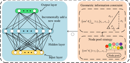
Figure 2: Network structure of ICA.

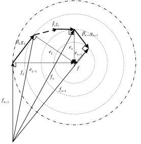
Figure 3: Spatial geometry construction process of ICA.

III-C Algorithm Implementations

In this section, two different algorithm implementations, termed ICA and ICA+, will be reported. The network structure and spatial geometry construction process of ICA are shown in Fig. 2 and Fig. 3.

III-C1 ICA

For a target function $f:{R^{d}}\to{R^{m}}$, assume that an ICA with ${L-1}$ hidden nodes has been constructed, i.e., ${f_{L-1}}=\sum\nolimits_{j=1}^{L-1}{{\beta_{j}}{g_{j}}\left({\omega_{j}^{\rm{T}}\cdot x+{b_{j}}}\right)}$. If the generated ${g_{L}}$ makes the interpretable geometric information constraint Eq. (11) hold, and the output weights are given by

$$\beta{\rm{=}}\arg\mathop{\min}\limits_{\beta}\left\|{f-\sum\limits_{j=1}^{L}{{\beta_{j}}{g_{j}}}}\right\|$$ (12)

Then, we have that ${\lim_{L\to\infty}}\left\|{f-{f_{L}}}\right\|{\rm{=0}}$, where ${f_{L}}={f_{L-1}}+{\beta_{L}}{g_{L}}$.

Rearranging Eq.(12), the following matrix form results

$$\beta={H^{\dagger}}{f_{L}}$$ (13)

where $\beta=\left[{{\beta_{1}},{\beta_{2}},...,{\beta_{L}}}\right]^{\rm{T}}$, $H=\left[{{g_{1}},{g_{2}},...,{g_{L}}}\right]$, ${H^{\dagger}}$ denotes the Moore-Penrose generalized inverse of $H$.

Remark 3: The calculation of the Moore${-}$Penrose generalized inverse involves the SVD, which will greatly increase computational cost. The problem is even more acute when dealing with large-scale data modeling tasks. To solve this problem, using the iteration theory of Greville[21, 22, 23], the ICA is extended to a lightweight version, called ICA+.

III-C2 ICA+

For a target function $f:{R^{d}}\to{R^{m}}$, assuming that the ICA with ${L-1}$ hidden nodes has been constructed, i.e., ${f_{L-1}}=\sum\nolimits_{j=1}^{L-1}{{\beta_{j}}{g_{j}}\left({\omega_{j}^{\rm{T}}\cdot x+{b_{j}}}\right)}$. If the generated ${g_{L}}$ makes Eq. (11) holds. Let $H_{L-1}=\left[{{g_{1}},{g_{2}},...,{g_{L-1}}}\right]$ denote the output weights matrix of the hidden layer with $L-1$ nodes. ${H_{L}}{\rm{=}}\left[{{H_{L{\rm{-}}1}}{\rm{}}{g_{L}}}\right]$ represents the output weights matrix of the hidden layer with $L$ nodes. Based on the iteration theory of Greville, $H_{L}^{\dagger}$ can be obtained by

$$H_{L}^{\dagger}{\rm{=}}\left[{\begin{array}[]{*{20}{c}}{H_{L-1}^{\dagger}-{d_{L}}b_{L}^{\rm{T}}}\\ {b_{L}^{\rm{T}}}\end{array}}\right]$$ (14)

where ${d_{L}}=H_{L-1}^{\dagger}{g_{L}}$, ${c_{L}}={h_{L}}-{H_{L-1}}{d_{L}}$, $b_{L}^{\rm{T}}=\left\{{\begin{array}[]{*{20}{c}}{{{\left({{c_{L}}}\right)}^{\dagger}}}&{\begin{array}[]{*{20}{c}}{if}&{{c_{L}}\neq 0}\end{array}}\\ {{{\left({1+d_{L}^{\rm{T}}{d_{L}}}\right)}^{-1}}d_{L}^{\rm{T}}H_{L-1}^{\rm{+}}}&{\begin{array}[]{*{20}{c}}{if}&{{c_{L}}=0}\end{array}}\end{array}}\right.$.

Then, the output weights can be derived as

$$\beta{\rm{=}}\left[{\begin{array}[]{*{20}{c}}{{\beta^{previous}}-{d_{L}}b_{L}^{\rm{T}}f}\\ {b_{L}^{\rm{T}}f}\end{array}}\right]$$ (15)

where ${\beta^{previous}}$ denotes the output weights before a new hidden node is added. The specific implementation steps of ICA and ICA+ are shown in the pseudocode.

Algorithm ICA(+)

  

  Initialize

  $x=\left\{{{x_{1}},{x_{2}},...,{x_{N}}}\right\}$, ${x_{i}}\in{R^{d}}$ is the input and $f{\rm{=}}\left\{{{f_{1}},{f_{2}},...,{f_{N}}}\right\}$, ${f_{i}}\in{R^{m}}$ is the output; ${T_{\max}}$ denotes the maximum times of random configuration; ${L_{\max}}$ denotes the maximum number of iteration; $\ell$ is the expected error tolerance, $\zeta{\rm{=}}\left\{{{\lambda_{\min}}:\lambda:{\lambda_{\max}}}\right\}$ is a set of positive scalars; ${e_{0}}=f$, $0<r<1$, $\Omega$, $W$, $L=1$.

  While $L\leq{L_{max}}$ or $\left\|{\left.{{e_{0}}}\right\|}\right.>\ell$, do

         Hidden Parameters Configuration

         For $\lambda\in\zeta$, do

              For $k=1,2,...,{T_{\max}}$, do

                   Randomly assign the input weights ${\omega_{L}}$ and the bias ${b_{L}}$ from ${\left[{-\lambda,\lambda}\right]^{d}}$ and $\left[{-\lambda,\lambda}\right]$, respectively;

                   Calculate ${g_{L}}$, ${\cos}{\theta_{L-1}}$ based on ${g_{L}}={g_{L}}\left({\left({\omega_{L}^{\rm{T}}\cdot x+{b_{L}}}\right)}\right)$ and $\frac{{\left\langle{{e_{L-1}},{g_{L}}}\right\rangle}}{{\left\|{{e_{L-1}}}\right\|\cdot\left\|{{g_{L}}}\right\|}}$;

                   Save ${\omega_{L}}$ and ${b_{L}}$ in $W$;

              End For.

              Calculate $\tau$ and ${\gamma_{L}}$;

              If ${\left({{{\cos}^{2}}{\theta_{L-1}}}\right)}\geq{\gamma_{L}}\left\langle{{e_{L-1}},{e_{L-1}}}\right\rangle$, do

                   Find $w_{L}^{*},{\rm{}}b_{L}^{*}$ that maximize ${\cos^{2}}{\theta_{L-1}}$ in $W$;

                   Set ${H_{L}}=\left[{{g_{1}},{g_{2}},...,{g_{L}}}\right]$;

              Else

                   Renew $\sigma:=\sigma+rand\left({1-\sigma,1}\right)$;

                   Returns and regenerates the hidden parameters;

              End If.

         End For.

         Output Weight Evaluation

         Calculate $\beta$ using Eq. (13) (ICA) or Eq. (15) (ICA+);

         Obtain ${e_{L}}=f-{H_{L}}\beta$;

         Update ${e_{0}}={e_{L}}$ and $L=L+1$;

  End While.

IV EXPERIMENTAL RESULTS

In this section, we present the performance of the proposed ICA and ICA+ as well as IRWNNs, and CIRWN on a function approximation dataset, six benchmark datasets, an ore grinding semi-physical simulation platform, and a gesture recognition system. The function approximation dataset was randomly generated by Eq. (16) defined on [0, 1]. The specifications of the seven datasets can be found in TABLE I. In addition, the experimental parameters of all algorithms are summarized in TABLE II. The above experimental parameter settings are the best solutions obtained from multiple experiments.

$$f\left(x\right)=\frac{1}{{({{(x-0.3)}^{2}}+0.01)}}+\frac{1}{{({{(x-0.9)}^{2}}+0.04)}}-6$$ (16)

where $x\in\left[{0,1}\right]$.

All the comparing experiments are implemented on MATLAB 2020a running on a PC with 3.00 GHz Core i7 CPU and 8 GB RAM. Each experiment is repeated 30 times, and the average of the 30 experiments is set as the final reported result. The sigmoid function $g\left(u\right)=\frac{1}{{1+\exp\left({-u}\right)}}$ is employed as the activation function of these four randomized algorithms. In addition, modeling accuracy, root mean squares error (RMSE), and efficiency (the time spent on building the network) were employed to measure the performance of all randomized algorithms.

$${\rm{RMSE}}=\sqrt{\frac{1}{N}\sum\limits_{i=1}^{N}{{{\left({{f_{i}}-{{\tilde{f}}_{i}}}\right)}^{2}}}}$$ (17)

where ${{f_{i}}}$ denotes the real value of the output, ${{{\tilde{f}}_{i}}}$ is the prediction, $N$ is the number of the input.

TABLE I: Description of Seven Benchmark Datasets

Datasets	Training data	Testing data	Features	Output
Function	2000	400	1	1
Compactiv	6144	2048	21	1
Concrete	700	330	8	1
Winequality	1120	479	11	1
Iris	105	45	4	3
HAR	7352	2947	561	6
Sement	1617	693	20	6

TABLE II: Experimental Parameters

Datasets	IRWNNs		CIRWN/ICA/ICA+		$\ell$	${L_{\max}}$
	$\lambda$	${T_{\max}}$	$\zeta$	${T_{\max}}$
Function	150		150:10:200		0.05	200
Compactiv	0.5		0.5:0.1:5		0.05	100
Concrete	1		1:1:10		0.05	200
Winequality	0.5	1	0.5:0.1:5	20	0.05	100
Iris	1		0.5:0.1:5		0.05	50
HAR	0.5		0.5:0.1:5		0.05	500
Sement	150		150:10:200		0.05	100

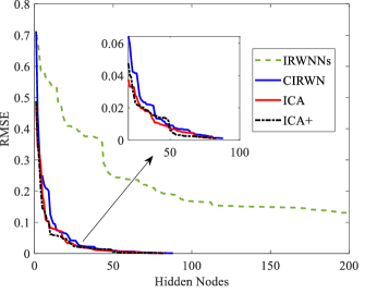
Figure 4: Convergence curve of RMSE for the ICA, ICA+, CIRWN and IRWNNs.

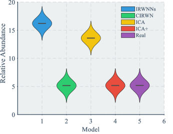
Figure 5: KDF of the ICA, ICA+, CIRWN and IRWNNs.

IV-A Results

IV-A1 Function Approximation Dataset

Fig. 4 shows the convergence performance of RMSE for the ICA, ICA+, IRWNNs, and CIRWN on the function approximation dataset. From Fig. 4, it can be observed that the convergence of RMSE based on ICA, ICA+ and CIRWN can be reached after dozens of hidden nodes. In addition, both ICA and ICA+ require fewer hidden nodes to achieve the RMSE convergence. These results show that the proposed two randomized algorithms have obvious advantages in compact structure. Fig. 5 shows the kernel density function (KDF) of the estimated error when the models achieve the expected error tolerance. It can be seen from Fig. 5 that the ICA and the ICA+ perform better than the IRWNNs and the CIRWN due to the KDF of ICA and ICA+ is approximating the real data distribution. This means that the proposed ICA and ICA+ have better prediction ability. Fig. 6 describes the different parameters $\lambda$ influence on the KDF performance of ICA. It is evident that different $\lambda$ have favorable or unfavorable effects on the KDF performance of ICA. This shows that $\lambda$ is an important parameter for the KDF performance of ICA. Therefore, to achieve better KDF performance, $\lambda$ should not remain fixed.

TABLE III: Comparison with Four Algorithms in Terms of Time, Training RMSE and Testing RMSE on the benchmark datasets

Dataset	Training time Training RMSE Testing RMSE
	IRWNNs			CIRWN			ICA			ICA+
Compactiv	0.234s	0.253	0.257	1.216s	0.062	0.071	1.122s	0.062	0.072	0.580s	0.062	0.072
Concrete	0.278s	0.253	0.256	1.09s	0.106	0.206	0.852s	0.095	0.206	0.281s	0.134	0.232
Winequality-read	0.120s	0.308	0.308	0.314s	0.150	0.159	0.287s	0.150	0.185	0.069s	0.150	0.185
Iris	0.059s	0.160	0.239	0.098s	0.019	0.043	0.080s	0.017	0.042	0.022s	0.018	0.043
HAR	56.401s	0.117	0.149	123.90s	0.016	0.055	123.177s	0.014	0.036	40.259s	0.014	0.038
Segment	0.318s	0.277	0.479	0.690s	0.199	0.218	0.536s	0.194	0.216	0.265s	0.193	0.216

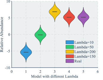
Figure 6: Impact of different $\lambda$ on KDF.

IV-A2 Benchmark Datasets

In this section, the performance of the ICA, ICA+, IRWNNs, and CIRWN is measured on six benchmark datasets. These benchmark datasets are mainly from KEEL and UCI, and their details can be observed in TABLE I. The experimental parameter information of the four randomized algorithms are given in TABLE II. TABLE III shows the time, training RMSE and testing RMSE results of these four randomized algorithms on six benchmark datasets. As shown in TABLE III, the training RMSE of both ICA and ICA+ is lower than that of CIRWN on most datasets. This means that the interpretable geometric information constraint can help generate better quality hidden parameters. Meanwhile, when compared wth the ICA+, the ICA is weak in the testing and training RMSE performance. This is because ICA+ uses an iterative update method to obtain the output weights, which is very dependent on the quality of the output weights of the first hidden node. In contrast, ICA uses the Moore-Penrose generalized inverse method to obtain the output weights, which enables ICA to obtain the globally optimal output weights after each node is added.

When the same hidden nodes are added, the training time of the proposed ICA and ICA+ is lower than the training time of CIRWN, especially ICA+. Compared with ICA, ICA+ reduced the training time by 14.29%, 50.56%, 67.58%, 43.31%, 67.02%, and 75.96% on Iris, Segment, HAR, Compactiv, Concrete, and Winequality, respectively. Therefore, the ICA+ is superior to other randomized algorithms in terms of lightweight. Fig. 7 depicts the effect of the hidden node pool size ${T_{\max}}$ on the RMSE of ICA. It shows that too large or too small ${T_{\max}}$ leads to an increase in RMSE. It is worth noting that we do not show the training time. In fact, ${T_{\max}}$ is related to the efficiency of the network because it controls the number of hidden parameters obtained from the random interval. In our experiments, this parameter was set with careful trade-offs.

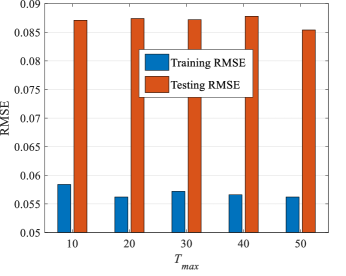
Figure 7: Impact of node pool on RMSE.

IV-B Hand Gesture Recognition Case

Hand Gesture recognition (HGR) is a hot topic in patter recognition due to its wide ranges of applications, such as virtual reality, health monitoring and smart homes[24]. In this section, we evaluate the performance of ICA and ICA+ based on our own developed HGR system. The HGR system framework is shown in Fig. 8, which includes both hardware module and software module. The hardware module consists of a gesture data acquisition and a data transmission shown in Fig. 9. The software module includes a feature extraction and a modeling and recognition shown in Fig. 10. In this section, a gesture dataset with a total sample size of 5136, feature number of 64 and category number of 24 was obtained through the feature extraction of the software module[25]. The dataset has been divided into the training dataset and the testing dataset.

IV-B1 Parameter Configuration

For IRWNNs, the random set of hidden parameters is fixed interval [-150,150]. The random parameters of the other three randomized algorithms is selected from a variable interval $\zeta{\rm{=}}\left\{{150:10:200}\right\}$. For ICA, ICA+, and CIRWN, the maximum number of iteration is set to ${L_{\max}}$ = 500, and the maximum times of random configuration is set to ${T_{\max}}$ = 20.

IV-B2 Comparison and Discussion

The average RMSE of four algorithms based on thirty times of experiments on the HGR testing dataset is displayed in Fig. 11. It can be found that the ICA and ICA+ have good stability performance in terms of RMSE. As can be seen from Fig. 11, the difference between the maximum RMSE and the minimum RMSE for IRWNNs and CIRWN is 0.15 and 0.02, respectively. TABLE IV shows the experimental results of the IRWNNs, ICA, ICA+, and CIRWN on the HGR system. It can be seen from TABLE IV that compared with IRWNNs and CIRWN, the ICA and ICA+ have a great advantage in terms of training time and classification accuracy. Based on the comparisons and analyzes of these results, we can conclude that the proposed ICA and ICA+ are more effective than IRWNNs and CIRWN for HGR tasks.

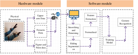
Figure 8: Framework diagram of gesture recognition system.

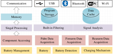
Figure 9: Hardware module.

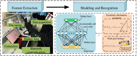
Figure 10: Software module.

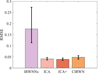
Figure 11: RMSE comparison of different algorithms.

TABLE IV: Performance Comparison of Four Algorithms on Gesture Recognition System

Algorithms	Training time	Accuracy	Nodes
IRWNNs	20.37s	82.43%	500
CIRWN	41.63s	95.12%	500
ICA	40.79	96.10%	500
ICA+	14.68s	96.48%	500

IV-C Ore grinding Case

Ore grinding is the monomer dissociation between useful minerals and lode minerals, and its process is illustrated in Fig. 12[26]. The mechanisms of ore grinding are complicated and hard to establish a mathematical model. Therefore, it is essential to establish a soft sensor for monitoring the ore grinding. As TABLE V shows, there are five process variables that are chosen to establish the ore grinding model. These process variables are collected from the ore grinding semi-physical simulation platform (see Fig. 13) and 20000 training samples and 5000 test samples have been obtained. The purpose of constructing the soft sensor model of the ore grinding process is to achieve the following nonlinear mapping:

TABLE V: Description of Ore Griding Process Variables

Tags	Descriptions
${R_{1}}$	Fresh ore feed rate
${R_{2}}$	Mile inlet water flow rate
${R_{3}}$	Current through mill
${\alpha_{1}}$	Current through mill
${\alpha_{2}}$	Current through classifier

$${\rm{PS}}=f\left({{R_{1}},{R_{2}},{R_{3}},{\alpha_{1}},{\alpha_{2}}}\right)$$ (18)

IV-C1 Parameter Configuration

For IRWNNs, the random set of hidden parameters is fixed interval [-150,150]. The random parameters of the other three randomized algorithms are selected from a variable interval $\zeta{\rm{=}}\left\{{150:1:500}\right\}$. For ICA, ICA+, and CIRWN, the maximum number of iteration is set to ${L_{\max}}$ = 100, and the maximum times of random configuration is set to ${T_{\max}}$ = 20.

IV-C2 Comparison and Discussion

Fig. 14 shows the probability density function (PDF) of the estimation error when the model reaches the expected error tolerance for the four models. In particular, ICA and ICA+ share a PDF curve due to the similar result. It can be seen from Fig. 14 that the ICA and ICA+ have better than the other two models because the curve of ICA and ICA+ is approximately normal distribution comparing to IRWNNs and CIRWN. This means that the ICA and ICA+ have the best performance among ore grinding systems. Besides, TABLE VI shows the experimental results of the IRWNNs, ICA, ICA+, and CIRWN on the the ore grinding semi-physical simulation platform. The modeling time of ICA, ICA+, CIRWN, and IRWNNs are 3.29s, 1.91s, 3.93s, and 0.57s, respectively. Comparing with ICA and CIRWN, ICA+ achieves the minimum training time while maintains the desired accuracy. When compared with the CIRWN, the ICA is strong in training time. It follows from the above experiment results and analysis that the proposed ICA and ICA+ can obtain superior performance in terms of generalization and training time. Moreover, these remarkable merits make the ICA and ICA+ be a very nice choice for the ore grinding.

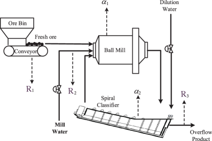
Figure 12: Flow chart of an ore grinding PS.

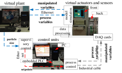
Figure 13: Structure of the Semi-physical Simulation Platform.

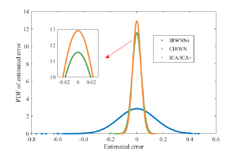
Figure 14: PDF of IRWNNs, ICA, ICA+, and CIRWN.

TABLE VI: Performance Comparison of Four Algorithms on Ore Grinding Semi-physical Simulation Platform

Algorithms	Training time	Accuracy	Nodes
IRWNNs	0.57s	85.89%	100
CIRWN	3.93s	95.53%	100
ICA	3.29s	95.67%	100
ICA+	1.91s	95.81%	100

V Conclusion

In this paper, an interpretable constructive algorithm (ICA) is proposed to visualize the contribution of each hidden parameter on residual error to improve the interpretability of RWNNs predicted behavior. In ICA, the hidden parameters are randomly assigned by the interpretable geometric information constraint with node pool strategy. Further, ICA is extended to ICA+ in order to reduce the computational cost. In particular, the difference between ICA+ and ICA is that ICA+ uses a more lightweight and efficient iterative update method to evaluate the output weights, while ICA uses a globally optimal approach to evaluate the output weights. Experimental results on seven benchmark datasets, a hand gesture recognition system and an ore grinding semi-physical simulation platform show that ICA and ICA+ can effectively reduce computational consumption and have better network performance than other construction algorithms.

References

- [1] X. Meng, J. Tang and J.-F. Fei, “NOx emissions prediction with a brain-inspired modular neural network in municipal solid waste incineration processes,” in IEEE Transactions on Industrial Informatics., vol. 18, pp. 4622–4631, 2022.
- [2] Z.-Q. Geng, Z.-W. Chen, Q.-C. Meng and Y.-M. Han, “Novel transformer based on gated convolutional neural network for dynamic soft sensor modeling of industrial processes,” in IEEE Transactions on Industrial Informatics., vol. 18, pp. 1521–1529, 2022.
- [3] X.-F. Yuan, L. Li, Y.-L. Wang, “Nonlinear dynamic soft sensor modeling with supervised long short-term memory network,” in IEEE Transactions on Industrial Informatics., vol. 16, pp. 3168–3176, 2020.
- [4] H.-F. Zhang, Y. Dong, C.-X. Dou and G.-P. Hancke, “PBI based multi-objective optimization via deep reinforcement elite learning strategy for micro-grid dispatch with frequency dynamics,” in IEEE Transactions on Power Systems., vol. 38, pp. 488–498, 2023.
- [5] Y.-H. Jia, S. Kwong and R. Wang, “Applying exponential family distribution to generalized extreme learning machine,” in IEEE Transactions on Systems, Man, and Cybernetics: Systems., vol. 50, pp. 1794–1804, 2020.
- [6] Y.-H. Pao and Y. Takefuji, “Functional-link net computing: theory, system architecture, and functionalities,” in Computer., vol. 25, pp. 76–79, 1992.
- [7] Y.-H. Pao, G.-H. Park, D.-J. Sobajic, “Learning and generalization characteristics of the random vector Functional-link net,” in Neurocomputing., vol. 6, pp. 163–180, 1994.
- [8] B. Igelnik and Y.-H. Pao, “Stochastic choice of basis functions in adaptive function approximation and the functional-link net,” in IEEE Transactions on Neural Networks., vol. 6, pp. 1320–1329, 1995.
- [9] F. Han, J. Jiang, Q. H. Ling, and B. Y . Su, “Stochastic choice of basis functions in adaptive function approximation and the functional-link net,” in Neurocomputing., vol. 335, pp. 261–273, 2019.
- [10] X. Wu, P. Rozycki and B. M. Wilamowski, “A hybrid constructive algorithm for single-layer feedforward networks learning,” in IEEE Transactions on Neural Networks and Learning Systems., vol. 26, pp. 1659–1668, 2015.
- [11] L.-Y. Ma and K. Khorasani, “Insights into randomized algorithms for neural networks: Practical issues and common pitfalls,” in IEEE Transactions on Neural Networks and Learning Systems., vol. 16, pp. 821–833, 2005.
- [12] G. Feng, G.-B. Huang, Q. Lin and R. Gay, “Error minimized extreme learning machine with growth of hidden nodes and incremental learning,” in IEEE Transactions on Neural Networks., vol. 20, pp. 1352-1357, 2009.
- [13] Dudek G, “A constructive approach to data-driven randomized learning for feedforward neural networks,” in Applied Soft Computing., vol. 112, pp. 107797, 2021.
- [14] S. Ferrari and R.-F. Stengel, “Smooth function approximation using neural networks,” in IEEE Transactions on Neural Networks., vol. 16, pp. 24–38, 2005.
- [15] I.-Y. Tyukin and D.-V. Prokhorov, “Feasibility of random basis function approximators for modeling and control,” in 2009 IEEE Control Applications, (CCA) & Intelligent Control., 2009, pp. 1391–1396.
- [16] D.-H. Wang and M. Li, “Stochastic configuration networks: fundamentals and algorithms,” in IEEE Transactions on Cybernetics., vol. 47, pp. 3466–3479, 2017.
- [17] Dudek G, “Generating random weights and biases in feedforward neural networks with random hidden nodes,” in Information Sciences., vol. 481, pp. 33-56, 2019.
- [18] Q.-J. Wang, W. Dai, P. Lin and P. Zhou, “Compact incremental random weight network for estimating the underground airflow quantity,” in IEEE Transactions on Industrial Informatics., vol. 13, pp. 426–436, 2022.
- [19] M. Islam, D.-T. Anderson, A.-J. Pinar, T.-C. Havens, G. Scott and J.-M. Keller, “Enabling explainable fusion in deep learning with fuzzy integral neural networks,” in IEEE Transactions on Fuzzy Systems., vol. 28, pp. 1291–1300, 2020.
- [20] H. Sasaki, Y. Hidaka and H. Igarashi, “Explainable deep neural network for design of electric motors,” in IEEE Transactions on Magnetics., vol. 57, pp. 1–4, 2021.
- [21] C.-L.-P. Chen and Z.-L. Liu, “Broad learning system: An effective and efficient incremental learning system without the need for deep architecture,” in IEEE Transactions on Neural Networks and Learning Systems., vol. 29, pp. 10–24, 2018.
- [22] S.-L. Issa, Q.-M. Peng and X.-G. You, “Emotion classification using EEG brain signals and the broad learning system,” in IEEE Transactions on Systems, Man, and Cybernetics: Systems., vol. 51, pp. 7382–7391, 2021.
- [23] L. Cheng, Y. Liu, Z.-G. Hou, M. Tan, D. Du and M. Fei, “A rapid spiking neural network approach with an application on hand gesture recognition,” in IEEE Transactions on Cognitive and Developmental Systems., vol. 13, pp. 151–161, 2021.
- [24] H. Cheng, L. Yang and Z. Liu, “Survey on 3D hand gesture recognition,” in IEEE Transactions on Circuits and Systems for Video Technology., vol. 26, pp. 1659–1673, 2016.
- [25] G. Yuan, X. Liu, Q. Yan, S. Qiao, Z. Wang and L. Yuan, “Hand gesture recognition using deep feature fusion network based on wearable sensors,” in IEEE Sensors Journal., vol. 21, pp. 539–547, 2021.
- [26] W. Dai, X.-Y. Zhou, D.-P. Li, S. Zhu and X.-S. Wang, “Hybrid parallel stochastic configuration networks for industrial data analytics,” in IEEE Transactions on Industrial Informatics., vol. 18, pp. 2331–2341, 2022.