Random Discrete Probability Measures Based on Negative Binomial Process

Abstract

An important functional of Poisson random measure is the negative binomial process (NBP). We use NBP to introduce a generalized Poisson-Kingman distribution and its corresponding random discrete probability measure. This random discrete probability measure provides a new set of priors with more flexibility in nonparametric Bayesian models. It is shown how this random discrete probability measure relates to the nonparametric Bayesian priors such as Dirichlet process, normalized positive $\alpha$-stable process, Poisson-Dirichlet process (PDP), and others. An extension of the DP with its almost sure approximation is presented. Using our representation for NBP, we derive a new series representation for the PDP.

and

addr1Department of Mathematics and Statistics, University of Ottawa, Ottawa, Canada e1   e2

t3Corresponding author

1 Introduction

The Poisson random measure (or Poisson point process) relates to other important processes through its functionals. The setup for a general point process follows the exposition in Kallenberg (1983) and Resnick (1987, Ch.3). Let $(\mathbb{E},\mathscr{E})$ be a locally compact space with a countable basis with its associated Borel $\sigma$-algebra and also let $(\mathbb{M},\mathscr{M})$ be the space of all point measures defined on $\mathbb{E}$ with its associated $\sigma$-algebra. A point process $\xi$ on $\mathbb{E}$ is a measurable map from the probability space $(\Omega,\mathcal{F},P)\to(\mathbb{M},\mathscr{M})$. It is well known that the probability law of a process is uniquely determined by its Laplace functional. The Laplace functional of the point process $\xi$ is defined by

$$\Psi_{\xi}(f)=E(e^{-\xi(f)})=\int_{m\in\mathbb{M}}\mathrm{exp}\left\{-\int_{\mathbb{E}}f(x)m(dx)\right\}P(\xi\in\mathrm{d}m)$$

where $f:\mathbb{E}\to[0,\infty)$ is measurable.

A point process $\xi$ on $(\mathbb{E},\mathscr{E})$ is called a Poisson random measure with mean measure $\mu$, denoted by PRM$(\mu),$ if its random number of points in a set $A\in\mathscr{E}$ has a Poisson distribution with parameter $\mu(A)$ and the numbers of points in disjoint sets are independent random variables. It can be shown that the Laplace functional of a PRM$(\mu)$ is given by

$$\Psi_{\xi}(f)=\mathrm{\exp}\left\{-\int_{\mathbb{E}}(1-e^{-f(x)})\mu(\mathrm{d}x)\right\}.$$ (1.1)

The following straightforward proposition derives a representation for the Poisson random measure with Lebesgue mean measure. There are many different ways to show this result. Since the recursive technique introduced in Banjevic et al. (2002) is helpful in other similar situations, we present it here.

Proposition 1.1.

Let $\xi\sim\mathrm{PRM}(\lambda)$ where $\lambda$ is the Lebesgue measure on $[0,\infty)$. Then $\xi$ can be written as follows

$$\xi=\sum_{i=1}^{\infty}\delta_{\Gamma_{i}},$$ (1.2)

where

$$\Gamma_{i}=E_{1}+\cdots+E_{i},$$

and $(E_{i})_{i\geq 1}$ is a sequence of independent and identically distributed (i.i.d.) random variables with an exponential distribution of mean 1. Throughout this paper, $\delta_{X}$ denotes the Dirac measure at $X$, i.e. $\delta_{X}(B)=1$ if $X\in B$ and $0$ otherwise.

Proof.

For any $t\geq 0$, define

$$\xi_{t}=\sum_{i=1}^{\infty}\delta_{\Gamma_{i}+t}$$

such that $\xi_{0}=\xi$. Now, for any nonnegative function $f$,

$$\Psi_{\xi_{t}}(f) =E(e^{-\xi_{t}(f)})=E(e^{-\sum_{i=1}^{\infty}f(\Gamma_{i}+t)})$$

$$=E(E(e^{-\sum_{i=1}^{\infty}f(\Gamma_{i}+t)}|\Gamma_{1}=s))$$

$$=\int_{0}^{\infty}e^{-f(s+t)}E(e^{-\sum_{i=1}^{\infty}f(\Gamma_{i}+s+t)})e^{-s}\mathrm{d}s$$

$$=\int_{0}^{\infty}e^{-f(s+t)}\Psi_{\xi_{s+t}}(f)e^{-s}\mathrm{d}s.$$

Using the change of variable $s+t=v$ and multiplying both sides by $e^{-t}$, we get

$$e^{-t}\Psi_{\xi_{t}}(f)=\int_{t}^{\infty}e^{-f(v)}\Psi_{\xi_{v}}(f)e^{-v}\mathrm{d}v.$$

Differentiating both sides with respect to $t$, we get

$$-e^{-t}\Psi_{\xi_{t}}(f)+e^{-t}\frac{\partial\Psi_{\xi_{t}}(f)}{\partial t} =-e^{-f(t)}\Psi_{\xi_{t}}(f)e^{-t}$$

$$\frac{\partial\Psi_{\xi_{t}}(f)}{\partial t}\frac{1}{\Psi_{\xi_{t}}(f)} =1-e^{-f(t)}$$

$$\Psi_{\xi_{t}}(f) =\mathrm{exp}\left(-\int_{t}^{\infty}(1-e^{-f(s)})\mathrm{d}s\right).$$

Now, take $t=0$ to get

$$\Psi_{\xi_{0}}(f) =\mathrm{exp}\left(-\int_{0}^{\infty}(1-e^{-f(s)})\mathrm{d}s\right)$$

which equals (1.1) with $\mu(\mathrm{d}s)=\lambda(\mathrm{d}s)=\mathrm{d}s$. ∎

Applying Proposition 2.1 and 2.2 of Resnick (1986) on $\mathrm{PRM}(\lambda)$ defined in (1.2), we can derive useful PRMs which in turn lead to other processes with applications in nonparametric Bayesian inference. First, take $T(x)=L^{-1}(x)$ where $L:(0,\infty)\to(0,\infty)$ is a decreasing bijection such that $\sum_{i=1}^{\infty}L^{-1}(\Gamma_{i})<\infty$, and

$$L^{-1}(y)=\inf\{x>0:L(x)\geq y\}.$$

Also, let $(\zeta_{i})_{i\geq 1}$ be a sequence of i.i.d. random elements in a Polish space $\mathbb{E}$ with a probability measure $H$ independent from $(\Gamma_{i})_{i\geq 1}$. Then we simply find that

$$\sum_{i=1}^{\infty}\delta_{L^{-1}(\Gamma_{i})} \sim\mathrm{PRM}(L),$$ (1.3)

$$\sum_{i=1}^{\infty}\delta_{(\zeta_{i},L^{-1}(\Gamma_{i}))} \sim\mathrm{PRM}(H\times L).$$ (1.4)

For example, $\sum_{i=1}^{\infty}\delta_{\Gamma_{i}^{-1/\alpha}}$ follows a PRM$(L)$ with

$$L(x)=x^{-\alpha}=\int_{x}^{\infty}\alpha u^{-\alpha-1}\mathrm{d}u,~{}x>0,~{}\alpha\in(0,1).$$ (1.5)

Throughout this paper, we use the function $L$ also as a measure with notation $L(\mathrm{d}x)=\mathrm{d}L(x)$. In fact, (1.5) denotes the Lévy measure of the $\alpha$-stable random variable $S_{\alpha}=\sum_{i=1}^{\infty}\Gamma_{i}^{-1/\alpha}.$ Notice that since $\Gamma_{i}/i\stackrel{{\scriptstyle a.s.}}{{\longrightarrow}}1$, $S_{\alpha}$ converges for $\alpha\in(0,1).$

As another example, for $\theta>0$ and $x>0$, take

$$L(x)=\theta\int_{x}^{\infty}u^{-1}e^{-u}\mathrm{d}u.$$ (1.6)

Then a functional of the random measure (1.4) given by $Q=\sum_{i=1}^{\infty}L^{-1}(\Gamma_{i})\delta_{\zeta_{i}},$ is a gamma process denoted by GaP$(\theta,H)$. This means that for disjoint sets $A_{1},\ldots,A_{k}$, the random variables $\{Q(A_{i})\}_{1\leq i\leq k}$ are independent and $Q(A_{i})$ has a gamma distribution with shape parameter $\theta H(A_{i})$ and scale parameter of $1$. Independence follows since $Q$ is a pure jump Lévy process. See Ishwaran and Zarepour (2002) for more details. This finite random measure is self-normalized as follows

$$P_{\theta,H}(\cdot)=\sum_{i=1}^{\infty}\frac{L^{-1}(\Gamma_{i})}{\sum_{i=1}^{\infty}L^{-1}(\Gamma_{i})}\delta_{\zeta_{i}}(\cdot)$$ (1.7)

by Ferguson (1973) to define the Dirichlet process DP$(\theta,H)$ to use it as a prior on the space of all probability measures on $\mathbb{E}$. The Dirichlet process is known as the cornerstone of the nonparametric Bayesian analysis. There has been an extensive effort to provide some generalizations and alternatives for this process; see for example, Pitman and Yor (1997), and Lijoi et al. (2005). Also, see Ishwaran and Zarepour (2002) and Zarepour and Al-Labadi (2012) for some alternative representations and approximations of this process.

Another important distribution which is resulted from a PRM is the Poisson-Kingman distribution. Consult Kingman (1975) and Pitman (2003) for properties and applications of this distribution. The vector of the normalized points of the PRM defined in equation (1.3), which we call them Poisson-Dirichlet weights, will follow a Poisson-Kingman distribution denoted by PK$(L)$, i.e.

$$\left(\frac{L^{-1}(\Gamma_{1})}{\sum_{i=1}^{\infty}L^{-1}(\Gamma_{i})},\frac{L^{-1}(\Gamma_{2})}{\sum_{i=1}^{\infty}L^{-1}(\Gamma_{i})},\ldots\right)\sim\mathrm{PK}(L)$$ (1.8)

defines a random discrete distribution on the infinite dimensional simplex $\nabla_{\infty}:=\{(x_{1},x_{2},\ldots):x_{i}\geq 0,i=1,2,\ldots,\sum_{i=1}^{\infty}x_{i}=1\}$. As a particular case, if in (1.8) we take $L$ as the gamma Lévy measure given in (1.6), then the Poisson-Dirichlet weights (1.8) are also said to have Poisson-Dirichlet distribution with parameter $\theta$, which we denote by $\mathrm{PD}(0,\theta)$. Also, as another special case, if in (1.8) one takes $L$ as the $\alpha$-stable Lévy measure given in (1.5), then the corresponding Poisson-Dirichlet weights (1.8) are also said to have Poisson-Dirichlet distribution with parameter $\alpha$, which we denote by $\mathrm{PD}(\alpha,0)$. Additionally, the random probability measure (1.7) is called a normalized $\alpha$-stable process if we employ the later Poisson-Dirichlet weights. See Ishwaran and James (2001).

Equivalently, a Poisson-Kingman distribution can be constructed using subordinators. Let $(X_{t})_{t\geq 0}$ be a subordinator with Lévy measure $L$ and write $(\Delta X_{t}:=X_{t}-X_{t-})_{t>0}$ for the jump process of $X_{t}$, and $\Delta X_{t}^{(1)}\geq\Delta X_{t}^{(2)}\geq\cdots$ for the ordered jumps up till time $t>0$. Then

$$\left(\frac{\Delta X_{t}^{(1)}}{X_{t}},\frac{\Delta X_{t}^{(2)}}{X_{t}},\ldots\right)\sim\mathrm{PK}(tL).$$

We saw how using a PRM, the Poisson-Kingman distribution (1.8) is obtained and consequently how the random discrete probability measure (1.7) can be constructed simply by using the Poisson-Dirichlet weights of the Poisson-Kingman distribution. In the rest of the paper, we will generalize the Poisson-Kingman distribution and the resulting random discrete probability measure by utilizing the negative binomial process instead of PRM. The negative binomial process representation which we use here is itself constructed directly from a PRM, unlike the representation in Ipsen and Maller (2017) where the negative binomial process is constructed from a trimmed subordinator.

The paper is organized as follows. In section 2, we derive the negative binomial process as a functional of a PRM and then using this process, we generalize the random discrete probability measure (1.7) and equivalently, the Poisson-Kingman distribution by adding a new parameter. As a special member of the family of the new defined random discrete probability measure, an extension of the Dirichlet process with its almost sure approximation is presented in section 3. Then, we present the general structures of the posterior and predictive processes in section 4. A justification of the role of the parameter $r$ in clustering problem is given in section 5. In section 6, we derive a new series representation for the Poisson-Dirichlet process (Carlton, 1999), which is based on our new representation of the negative binomial process. In section 7, we provide a simulation study to compare the efficiency of our suggested approximation of the new series representation of the Poisson-Dirichlet process with other representations of this process that exist in the literature. Finally, a summary of the conclusions is given in the last section.

2 Negative Binomial Process

In this section, we will see how the negative binomial process (NBP) is derived directly as a functional of a PRM. Later, we use this process to define a more general form of the Poisson-Kingman distribution and its corresponding random discrete probability measure. First, we note that for any constant $c>0$, a simple use of Proposition 2.1 of Resnick (1986) shows that the process $\sum_{i=1}^{\infty}\delta_{\Gamma_{i}+c}$ is a PRM$(\lambda)$ on $\mathbb{E}=[c,\infty)$, and $\sum_{i=1}^{\infty}\delta_{\Gamma_{i}/c}$ follows PRM$(c\lambda)$ on $\mathbb{E}=[0,\infty)$. Now, for any nonnegative integer $r$ and setting $\Gamma_{0}=1,$ consider the random measure

$$\eta=\sum_{i=r+1}^{\infty}\delta_{\Gamma_{i}/\Gamma_{r}}.$$

First, note that conditional on $\{\Gamma_{r}=u\}$, the process $\eta$ follows PRM$(u\lambda)$ on $\mathbb{E}=(1,\infty)$. So, the Laplace functional of $\eta$ is

$$E(e^{-\eta(f)})=E\left[E(e^{-\eta(f)}|\Gamma_{r}=u)\right]$$

$$=\int_{0}^{\infty}E(e^{-\eta(f)}|\Gamma_{r}=u)P(\Gamma_{r}\in\mathrm{d}u)$$

$$=\int_{0}^{\infty}\exp\left\{-\int_{1}^{\infty}(1-e^{-f(x)})u\lambda(\mathrm{d}x)\right\}P(\Gamma_{r}\in\mathrm{d}u)$$

$$=\int_{0}^{\infty}\exp\left\{-u\int_{1}^{\infty}(1-e^{-f(x)})\lambda(\mathrm{d}x)\right\}\frac{u^{r-1}e^{-u}}{\Gamma(r)}\mathrm{d}u$$

$$=\left(1+\int_{1}^{\infty}(1-e^{-f(x)})\lambda(\mathrm{d}x)\right)^{-r}.$$

This is in fact the Laplace functional of the negative binomial process defined in Gregoire (1984). We denote this process by NBP$(r,\lambda)$ and write $\eta\sim\mathrm{NBP}(r,\lambda)$ on $\mathbb{E}=(1,\infty)$. Following up on this example, we state the following theorem.

Theorem 2.1.

With a decreasing bijection $L:(0,\infty)\rightarrow(0,\infty)$ such that $\sum_{i=1}^{\infty}L^{-1}(\Gamma_{i})<\infty$, the following point process

$$\kappa=\sum_{i=r+1}^{\infty}\delta_{L^{-1}(\Gamma_{i}/\Gamma_{r})}$$ (2.1)

follows an $\mathrm{NBP}(r,L)$ on $\mathbb{E}=(0,L^{-1}(1))$.

The proof of the theorem is similar to what was presented above for the process $\eta$. Three important examples of $L$ are positive $\alpha$-stable, gamma, and inverse-Gaussian Lévy measures (Lijoi et al., 2005; Al-Labadi and Zarepour, 2013, 2014).

The NBP was defined in Gregoire (1984) only through its Laplace functional and no point process or subordinator representation was provided. As it is seen, the point process representation of NBP$(r,L)$ in (2.1) was derived directly as a functional of a PRM. In Ipsen and Maller (2017), a point process representation of the NBP, which equals to (2.1) in distribution, was derived using ordered jumps of a trimmed subordinator. If $(X_{t})_{t\geq 0}$ is a subordinator with Lévy measure $L$, by writing $(\Delta X_{t}:=X_{t}-X_{t-})_{t>0}$ for the jump process of $X_{t}$, and $\Delta X_{t}^{(1)}\geq\Delta X_{t}^{(2)}\geq\cdots$ for the ordered jumps at $t>0$, then the point process $\mathbb{B}^{(r)}=\sum_{i=1}^{\infty}\delta_{J_{r}(i)}$ follows NBP$(r,L)$ where $J_{r}(i)=\frac{\Delta X_{1}^{(r+i)}}{\Delta X_{1}^{(r)}},i=1,2,\ldots$.

Remark 2.1.

In the literature, the terminology “negative binomial process” is used for mathematically distinct concepts. Therefore, it seems necessary to clarify these concepts to avoid confusion. As stated before, in this paper, Ipsen and Maller (2017), and Ipsen et al. (2020, 2021, 2018), the negative binomial process is the one defined in Gregoire (1984). However, in engineering and computer science literature, some other definitions of the negative binomial process can be found. For example, the negative binomial process defined in Zhou and Carin (2015) is different from the one defined in Zhou et al. (2012) and Broderick et al. (2015), which all are different from Gregoire’s definition that we are considering in this paper.

Following Definition 2.1 of Ipsen and Maller (2017), by normalizing the points of the NBP defined in (2.1), the following sequence

$$\left(\frac{L^{-1}(\Gamma_{r+1}/\Gamma_{r})}{\sum_{i=r+1}^{\infty}L^{-1}(\Gamma_{i}/\Gamma_{r})},\frac{L^{-1}(\Gamma_{r+2}/\Gamma_{r})}{\sum_{i=r+1}^{\infty}L^{-1}(\Gamma_{i}/\Gamma_{r})},\ldots\right)$$ (2.2)

defines a 2-parameter random discrete distribution on the infinite dimensional simplex $\nabla_{\infty}$. In Ipsen and Maller (2017), this distribution is called a Poisson-Kingman distribution generated by NBP$(r,L)$ and is denoted by $\mathrm{PK}^{(r)}(L)$. In particular case of $\alpha$-stable Lévy measure, this process is denoted by $\mathrm{PD}_{\alpha}^{(r)}$. Clearly, it is seen that the random sequence (2.2) equals

$$\left(\frac{J_{r}(1)}{\sum_{i=1}^{\infty}J_{r}(i)},\frac{J_{r}(2)}{\sum_{i=1}^{\infty}J_{r}(i)},\ldots\right)$$

in distribution. Also, as pointed out in Ipsen and Maller (2017), an NBP$(r,L)$ can be characterized as a PRM with randomized intensity measure $\Gamma_{r}L$ where $\Gamma_{r}$ is a Gamma$(r,1)$ random variable, i.e. $\mathrm{PRM}(\Gamma_{r}L)\stackrel{{\scriptstyle d}}{{=}}\mathrm{NBP}(r,L)$. In other words, a gamma subordinated Lévy process $X_{\sigma_{r}}$ will follow an NBP$(r,L)$ where $(\sigma_{r})_{r>0}$ is an independent gamma subordinator having Lévy measure (1.6) with $\theta=1$. Then by the definition of the Poisson-Kingman distribution, the random sequence (2.2) will also equal in distribution to

$$\left(\frac{\Delta X_{\sigma_{r}}^{(1)}}{X_{\sigma_{r}}},\frac{\Delta X_{\sigma_{r}}^{(2)}}{X_{\sigma_{r}}},\ldots\right).$$ (2.3)

Definition 2.1.

Let $(\zeta_{i})_{i\geq 1}$ be i.i.d. random variables with values in $\mathbb{E}$ and common distribution $H$, then we may introduce the following random discrete probability measure on $E$ as a functional of (2.1) or using the sequence (2.2) as follows

$$P_{r,L,H}(\cdot)=\sum_{i=r+1}^{\infty}\frac{L^{-1}(\Gamma_{i}/\Gamma_{r})}{\sum_{i=r+1}^{\infty}L^{-1}(\Gamma_{i}/\Gamma_{r})}\delta_{\zeta_{i}}(\cdot).$$ (2.4)

We employ the notation $\mathrm{PKP}^{(r)}(H;L)$ for the distribution of the random discrete probability measure defined in (2.4) and we write $P_{r,L,H}\sim\mathrm{PKP}^{(r)}(H;L)$.

3 Extended Dirichlet Process and its Approximation

In the case $L$ is the $\alpha$-stable Lévy measure given in (1.5), $\mathrm{PK}^{(r)}(L)$ has been investigated thoroughly. For example, it is shown that how this distribution relates to other Poisson–Dirichlet models by letting $r\to\infty$ in Ipsen et al. (2020). Also, in Ipsen et al. (2018), this distribution is fitted to gene and species sampling data, demonstrating the utility of allowing the extra parameter $r$ in data analysis.

We may now take the probability measure (2.4) with $L$ as the gamma Lévy measure defined in (1.6) to develop a prior distribution on the space of all probability distributions. This prior would be a natural extension of the Dirichlet process (the Dirichlet process is recovered when $r=0$). In the following theorem, we provide an efficient approximation for our extended Dirichlet process.

Theorem 3.1.

Let $W_{n}$ be a random variable with distribution Gamma$(\alpha/n,1)$. Define

$$G_{n}(x)=\mathrm{Pr}(W_{n}>x)=\int_{x}^{\infty}\frac{1}{\Gamma(\alpha/n)}e^{-t}t^{\alpha/n-1}\mathrm{d}t$$

and

$$G_{n}^{-1}(y)=\mathrm{inf}\{x:G_{n}(x)\geq y\},~{}~{}0<y<1.$$

Let $L$ be the gamma Lévy measure (1.6) and $(\zeta_{i})_{i\geq 1}$ be a sequence of i.i.d. random variables with values in $\mathbb{E}$ and common distribution $H$, independent of $(\Gamma_{i})_{i\geq 1}$, then as $n\to\infty$

$$P_{n,r,H}=\sum_{i=r+1}^{n}\frac{G_{n}^{-1}\left(\frac{\Gamma_{i}}{\Gamma_{r}\Gamma_{n+1}}\right)}{\sum_{i=r+1}^{n}G_{n}^{-1}\left(\frac{\Gamma_{i}}{\Gamma_{r}\Gamma_{n+1}}\right)}\delta_{\zeta_{i}}\stackrel{{\scriptstyle a.s.}}{{\longrightarrow}}P_{r,L,H}=\sum_{i=r+1}^{\infty}\frac{L^{-1}\left(\frac{\Gamma_{i}}{\Gamma_{r}}\right)}{\sum_{i=r+1}^{\infty}L^{-1}\left(\frac{\Gamma_{i}}{\Gamma_{r}}\right)}\delta_{\zeta_{i}}$$

on $\mathbb{E}$ with respect to the weak topology.

Proof.

The proof is similar to that of Theorem 1 in Zarepour and Al-Labadi (2012) and the fact that $G_{n}^{-1}\left(\frac{x}{cn}\right)\stackrel{{\scriptstyle a.s.}}{{\longrightarrow}}L^{-1}\left(\frac{x}{c}\right)$. Consequently $G_{n}^{-1}\left(\frac{\Gamma_{i}}{\Gamma_{r}\Gamma_{n+1}}\right)\stackrel{{\scriptstyle a.s.}}{{\longrightarrow}}L^{-1}\left(\frac{\Gamma_{i}}{\Gamma_{r}}\right)$ by taking the constant $c=\Gamma_{r}$, $x=\Gamma_{i}$, and $n=\Gamma_{n+1}$ as $\Gamma_{n+1}/n\stackrel{{\scriptstyle a.s.}}{{\longrightarrow}}1$ when $n\to\infty$. ∎

Our proposed approximation has several advantages. For example, our representation avoids the use of an infinite sum and instead our finite many weights are simply the quantile functions of the Gamma$(\alpha/n,1)$ distribution evaluated at $1-\Gamma_{i}/\Gamma_{r}\Gamma_{n+1}$. In previous representation, it is necessary to calculate $L^{-1}$ which can not be written in a closed form. In addition, our introduced weights are stochastically decreasing contrary to stick-breaking weights in Ipsen and Maller (2017). A similar proposal for the Dirichlet process can be found in Zarepour and Al-Labadi (2012).

4 Posterior and Predictive Distribution

To develop a full Bayesian analysis, we can generalize $P_{r,L,H}$ defined in (2.4) by assuming that $r$ is a realization of a random variable $R$, on set of non-negative integers with an arbitrary probability mass function $\pi(r).$ Also for simplicity in notations, denote the weights of $P_{R,L,H}$ by $p_{i}$. Therefore, we can write

$$P_{R,L,H}=\sum_{i=R+1}^{\infty}p_{i}\delta_{\zeta_{i}}.$$

For given observations from $P_{R,L,H}$, the posterior and predictive distribution of the prior $P_{R,L,H}$ can be obtained from Ongaro and Cattaneo (2004) using a recursive method. This method obtains the posterior distribution for a general random discrete probability measure of the form

$$P=\sum_{i=1}^{M}p_{i}\delta_{\zeta_{i}},$$

where $M$ is an extended integer valued random variable with an arbitrary probability distribution $p(m).$ Moreover, conditionally on $M,~{}(p_{1},\ldots,p_{M})$ has an arbitrary distribution $Q_{M}$ on simplex $\nabla_{M}:=\{(x_{1},\ldots,x_{M}):x_{i}\geq 0,i=1,2,\ldots,M,\sum_{i=1}^{M}x_{i}=1\}$. The random positions $\zeta_{i}$’s are i.i.d. from a diffuse probability measure $H$ and are independent of all other random elements.

In our case, for $P_{R,L,H}$, we only need to change the role of $M$ with $R$, where similar results of Ongaro and Cattaneo (2004) follow easily. Following their procedure, we need to find the posterior distribution of random elements of $P_{R,L,H}$, i.e. $(R,\boldsymbol{p},\boldsymbol{\zeta})$ where $\boldsymbol{p}=(p_{R+1},p_{R+2},\ldots)$ and $\boldsymbol{\zeta}=(\zeta_{R+1},\zeta_{R+2},\ldots)$. The calculations for finding the posterior of $(R,\boldsymbol{p},\boldsymbol{\zeta})$ remain similar to the ones in Propositions 4 and 5 in Ongaro and Cattaneo (2004). The final summary is provided in the following theorem.

Theorem 4.1.

Let $\boldsymbol{X}=(X_{1},\ldots,X_{n})$ be a random sample of $n$ observations from $P_{R,L,H}$. The posterior process $P_{R,L,H}|\boldsymbol{X}$ can be represented as

$$\left(P_{R,L,H}|\boldsymbol{X}\right)=\sum_{i=1}^{k}\gamma_{i}^{\boldsymbol{X}}\delta_{X_{i}^{\ast}}+\sum_{i=R^{\boldsymbol{X}}+1}^{\infty}p_{i}^{\boldsymbol{X}}\delta_{\zeta_{i}},$$ (4.1)

where $X_{i}^{\ast}$s are the distinct values among the observations $\boldsymbol{X}$ and $R^{\boldsymbol{X}}$ and
$\boldsymbol{p}^{\boldsymbol{X}}=(\gamma_{1}^{\boldsymbol{X}},\ldots,\gamma_{k}^{\boldsymbol{X}},p_{R^{\boldsymbol{X}}+1}^{\boldsymbol{X}},p_{R^{\boldsymbol{X}}+2}^{\boldsymbol{X}},\ldots)$ denote the posteriors of $R$ and $\boldsymbol{p}$, respectively. The distribution of $R^{\boldsymbol{X}}$ and $\boldsymbol{p}^{\boldsymbol{X}}$ are obtained using a recursive method similar to Corollaries 3 and 4 in Ongaro and Cattaneo (2004).

To calculate the predictive distribution, take expectation of (4.1) to get

$$\mathrm{Pr}\left\{X_{n+1}\in A|\boldsymbol{X}\right\}=\sum_{i=1}^{k}c_{i}^{\boldsymbol{X}}\delta_{X_{i}^{\ast}}(A)+(1-c_{1}^{\boldsymbol{X}}-\cdots-c_{k}^{\boldsymbol{X}})H(A),$$

where $c_{i}^{\boldsymbol{X}}=E(\gamma_{i}^{\boldsymbol{X}})$ for $i=1,\ldots,k$.

5 Applications

Sufficiently large sample from a random discrete probability measure like (1.7) or (2.4), always includes ties with positive probability. Let $K_{n}=k\in\{1,\ldots,n\}$ be the number of distinct values among $n$ observations. Denote $X_{1}^{\ast},\ldots,X_{k}^{\ast}$ as distinct values among observations $X_{1},\dots,X_{n}$. Moreover, take $n_{j}=\sum_{i=1}^{n}I(X_{i}=X_{j}^{\ast})$ for $j=1,2,\ldots,k$. Obviously, $\sum_{j=1}^{k}n_{j}=n$. Note that we already saw how $k$ appeared in the posterior process (4.1). For the Dirichlet process, $k$ grows slowly as $n\to\infty.$ As it is shown in Korwar and Hollander (1973) and Pitman (2006), if

$$(X_{1},\ldots,X_{n})|P\sim P,~{}~{}P\sim\mathrm{DP}(\theta,H)$$

then

$$K_{n}/\log(n)\stackrel{{\scriptstyle a.s.}}{{\longrightarrow}}\theta~{}~{}\mathrm{as}~{}~{}n\to\infty.$$

It means that the random number of distinct values $K_{n}$ grows only in a logarithmic fashion. In other perspective, the Dirichlet process prior assigns most of the largest weights to its initial points. This property causes inflexibility in the use of the Dirichlet process as a prior mixing measure in nonparametric Bayesian hierarchical mixture models (or so called density estimation problem) when it is fitted to an over-dispersed data (Lo, 1984; Escobar and West, 1995; Ishwaran and James, 2001; Lijoi et al., 2005, 2007). Adding the new parameter $r$ and working with (2.4) instead of (1.7), will allow to remove those initial large probability weights and produce smother ones instead. For the Dirichlet case, Table 1 shows how choosing larger values for $r$ will lead to smoother probability weights in (2.4). Specially, in problems of density estimation similar to Lo (1984), this flexibility plays a crucial role but we do not address them here in this paper.

Table 1: The first ten probability weights in (2.4) when $L$ is the gamma Lévy measure (1.6) with $\theta=3$.

$r=0$	$r=3$	$r=5$	$r=10$
0.367597022	0.24369485	0.16427045	0.06353087
0.168573239	0.23947841	0.14319002	0.05886303
0.165457071	0.10281577	0.12842541	0.05418117
0.149080111	0.08716432	0.10524699	0.05112053
0.058821776	0.07639968	0.07391248	0.04858739
0.056183134	0.05990201	0.06339345	0.04626107
0.012551887	0.03862790	0.05279059	0.04349017
0.007812625	0.03184211	0.04298598	0.03795044
0.003792634	0.02524151	0.03705701	0.03606621
0.001971704	0.01939928	0.03245281	0.03021665

If we use $\alpha$-stable Lévy measure (1.5) in (1.7), this property is even more obvious. Since for the $\alpha$-stable random variable $S_{\alpha}=\sum_{i=1}^{\infty}\Gamma_{i}^{-1/\alpha},~{}\alpha\in(0,1),$ taking for example $\alpha=0.5$, the first four terms of $S_{1/2}$ have infinite variance which means that there is a huge fluctuation among the initial terms.

To present an alternative interpretation, notice that, the negative binomial distribution is preferred to the Poisson distribution when the data are over-dispersed. The variance of the negative binomial distribution is larger than its mean while for the Poisson distribution, both mean and variance are equal. Therefore, we expect that the random discrete probability measure (2.4) outperforms (1.7) as a prior mixing measure in nonparametric Bayesian hierarchical mixture models fitted to the over-dispersed data. Recall that the weights of (2.4) are the normalized points of the negative binomial process (2.1). However, the weights of (1.7) are the normalized points of the Poisson process (1.3) with a certain mean measure. We can observe that the weights in (2.4) decrease much slower than that of (1.7). See Table 1 for the case that $L$ is the gamma Lévy measure (1.6). This exhibits the mechanism that the random discrete probability measure (2.4) can naturally capture the over-dispersion better. In Ipsen et al. (2021, Theorem 2.1), the growth rate of $K_{n}(\alpha,r)=K_{n}$ is given rigorously for $\mathrm{PK}^{(r)}(L)$ when $L$ is the $\alpha$-stable Lévy measure. In other words, as $n\to\infty$

$$K_{n}/n^{\alpha}\stackrel{{\scriptstyle d}}{{\longrightarrow}}Y_{\alpha,r}.$$ (5.1)

See equation 2.8 in Ipsen et al. (2021) for the distribution of $Y_{\alpha,r}$. The growth rate $n^{\alpha}$ in (5.1) is equal to that of the Poisson-Dirichlet process (Pitman, 2006, Theorem 3.8) and the normalized generalized gamma process (Lijoi et al., 2007, Proposition 3). It is not surprising to see that the growth rates of $K_{n}$ for these processes are equal as all these processes belong to the greater family of the random discrete probability measure (2.4). We notice that the Poisson-Dirichlet process $\mathrm{PDP}(H;\alpha,\theta)$ is a particular case of the random discrete probability measure (2.4) with $r=\theta/\alpha$ and $L$ given in (6.2) and the normalized generalized gamma process is a particular case of the random discrete probability measure (2.4) with $r=0$ and $L$ given in (6.2). The Poisson-Dirichlet process and the normalized generalized gamma process have already been recommended in the literature to be exploited as mixing measures in nonparametric Bayesian hierarchical mixture models in order to allow the number of distinct values (the number of clusters) increases at a rate faster than that of the Dirichlet process. Therefore, the proposed random discrete probability measure (2.4) can be considered as a general alternative for the mixing measure in nonparametric Bayesian hierarchical mixture models fitted to the over-dispersed data.

6 A New Alternative Series Representation for the Poisson-Dirichlet Process

Using NBP, we can find another series representation rather than the stick-breaking representation for the Poisson-Dirichlet process. See Carlton (1999) for properties and applications of this process in nonparametric Bayesian analysis. For $0\leq\alpha<1,~{}\theta>-\alpha$, let $(\beta_{k})_{k\geq 1}$ be a sequence of independent random variables, where $\beta_{k}$ has the Beta$(1-\alpha,\theta+k\alpha)$ distribution. If we define

$$p^{\prime}_{1}=\beta_{1},~{}p^{\prime}_{i}=\beta_{i}\prod_{k=1}^{i-1}(1-\beta_{k}),~{}i\geq 2,$$

then the ranked sequence of $(p^{\prime}_{i})_{i\geq 1}$ denoted by $p_{1}\geq p_{2}\geq\ldots$ is said to have a Poisson-Dirichlet distribution with parameters $\alpha$ and $\theta$ denoted by PD$(\alpha,\theta)$ and we write $(p_{1},p_{2},\ldots)\sim\mathrm{PD}(\alpha,\theta).$ Also, note that $(p^{\prime}_{1},p^{\prime}_{2},\ldots)\sim\mathrm{GEM}(\alpha,\theta)$ with the notation used in Carlton (1999). Moreover, let $(\zeta_{i})_{i\geq 1}$ be i.i.d. random variables with values in $\mathbb{E}$ and common distribution $H$. Then the random probability measure

$$P_{\alpha,\theta,H}(\cdot)=\sum_{i=1}^{\infty}p_{i}\delta_{\zeta_{i}}$$ (6.1)

is called Poisson-Dirichlet process with parameters $\alpha,\theta,$ $H,$ and denoted by $\mathrm{PDP}(H;\alpha,\theta)$. As it is shown in Al-Labadi and Zarepour (2014, Lemma 2.1), the $p^{\prime}_{i}$’s are not strictly decreasing almost surely. Therefore, the stick-breaking representation (6.1) is inefficient for simulating this process due to failure in proper stopping rules. Another approach based on Proposition 22 of Pitman and Yor (1997), is proposed in Al-Labadi and Zarepour (2014) for simulating this process. This approach is more accurate than the method based on the stick-breaking representation, however, it includes more complex steps in its algorithm. In this section, we apply our new representation of NBP (2.1) to the Proposition 21 in Pitman and Yor (1997) to give a new representation for the Poisson-Dirichlet process. In section 7, we will show how simulating the Poisson-Dirichlet process using this representation is much more efficient while it avoids the shortcoming of the stick-breaking representation for simulation purposes. Moreover, our approach is less complex compared with the algorithm A in Al-Labadi and Zarepour (2014).

Now, following the Proposition 21 in Pitman and Yor (1997), for $\theta>0$ and $0<\alpha<1$, let $(X_{t})_{t\geq 0}$ be a subordinator having Lévy measure

$$L(x)=\frac{\alpha}{\Gamma(1-\alpha)}\int_{x}^{\infty}u^{-\alpha-1}e^{-u}\mathrm{d}u,~{}x>0$$ (6.2)

and let $(\sigma_{r})_{r>0}$ be an independent gamma subordinator. Then

$$\left(\frac{\Delta X_{T}^{(1)}}{X_{T}},\frac{\Delta X_{T}^{(2)}}{X_{T}},\ldots\right)\sim\mathrm{PD}(\alpha,\theta)~{}~{}\mathrm{if}~{}~{}T=\sigma_{\theta/\alpha}.$$ (6.3)

Comparing (6.3) with (2.3), we see that $\mathrm{PD}(\alpha,\theta)\stackrel{{\scriptstyle d}}{{=}}\mathrm{PK}^{(\theta/\alpha)}(L)$ with $L$ given in (6.2). Since $\mathrm{PD}(\alpha,\theta)\stackrel{{\scriptstyle d}}{{=}}\mathrm{PK}^{(\theta/\alpha)}(L)$ and (2.3) is equal to (2.2) in distribution, we can conclude $\mathrm{PDP}(H;\alpha,\theta)\stackrel{{\scriptstyle d}}{{=}}\mathrm{PKP}^{(\theta/\alpha)}(H;L)$ for $\theta>0,0<\alpha<1$ and $L$ in (6.2). In other words, the random probability measure

$$P_{r,L,H}(\cdot)=\sum_{i=r+1}^{\infty}\frac{L^{-1}(\Gamma_{i}/\Gamma_{r})}{\sum_{i=r+1}^{\infty}L^{-1}(\Gamma_{i}/\Gamma_{r})}\delta_{\zeta_{i}}(\cdot)$$ (6.4)

with $L$ given in (6.2) and $r=\theta/\alpha$ is distributed as either $\mathrm{PDP}(H;\alpha,\theta)$ or $\mathrm{PKP}^{(\theta/\alpha)}(H;L)$. Therefore, (6.4) provides another series representation for the Poisson-Dirichlet process for the case $\theta>0$ and $0<\alpha<1$ through a negative binomial process.

Note that $\mathrm{PK}^{(0)}(L)\stackrel{{\scriptstyle d}}{{=}}\mathrm{PD}(\alpha,0)$ for $0<\alpha<1$ and $L$ given in (1.5) and also, $\mathrm{PK}^{(0)}(L)\stackrel{{\scriptstyle d}}{{=}}\mathrm{PD}(0,\theta)$ for $\theta>0$ and $L$ given in (1.6). See Ipsen and Maller (2017) for stick-breaking representations of $\mathrm{PK}^{(r)}(L)$ with $L$ given in (1.5) and (1.6) when $r>0$.

7 Simulating a New Approximation of the Poisson-Dirichlet Process

By applying a truncation method on the new series representation of the Poisson-Dirichlet process $\mathrm{PDP}(H;\alpha,\theta)$ given in (6.4), we can approximate this process from

$$P_{n,r,L,H}(\cdot)=\sum_{i=r+1}^{n}\frac{L^{-1}(\Gamma_{i}/\Gamma_{r})}{\sum_{i=r+1}^{n}L^{-1}(\Gamma_{i}/\Gamma_{r})}\delta_{\zeta_{i}}(\cdot)$$ (7.1)

for $0<\alpha<1$, $\theta>0$, $r=\theta/\alpha$, and $L$ given in (6.2). We can suggest a stopping rule for choosing $n=n(\epsilon)$ as follows

$$n=\inf\left\{i:\frac{L^{-1}(\Gamma_{i}/\Gamma_{r})}{\sum_{j=r+1}^{i}L^{-1}(\Gamma_{j}/\Gamma_{r})}<\epsilon\right\}~{}~{}\mathrm{for}~{}\epsilon\in(0,1).$$

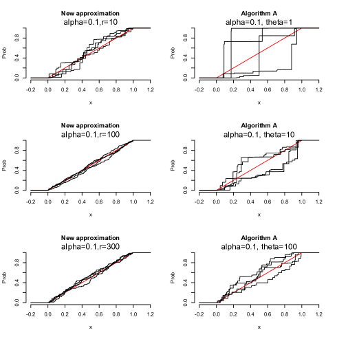
Figure 1: Sample paths of the two-parameter Poisson-Dirichlet process, where $H$ is the uniform distribution on $[0,1]$, $\alpha=0.1,$ and $\theta=1,10,100$. The red line denotes the cumulative distribution function of $H$.

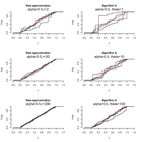
Figure 2: Sample paths of the two-parameter Poisson-Dirichlet process, where $H$ is the uniform distribution on $[0,1]$, $\alpha=0.5,$ and $\theta=1,10,100$. The red line denotes the cumulative distribution function of $H$.

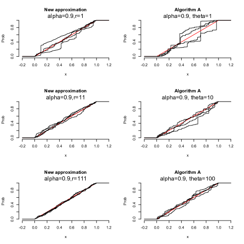
Figure 3: Sample paths of the two-parameter Poisson-Dirichlet process, where $H$ is the uniform distribution on $[0,1]$, $\alpha=0.9,$ and $\theta=1,10,100$. The red line denotes the cumulative distribution function of $H$.

Here, we compare the approximation given in (7.1) with the Algorithm A in Al-Labadi and Zarepour (2014) which is based on Proposition 22 of Pitman and Yor (1997). The superiority of this approximation over the corresponding stick-breaking approximation is presented, particularly for the cases when $\alpha$ is close to 1. Since the weights

$$\left(\frac{L^{-1}(\Gamma_{i}/\Gamma_{r})}{\sum_{i=r+1}^{n}L^{-1}(\Gamma_{i}/\Gamma_{r})}\right)_{r+1\leq i\leq n}$$

are strictly decreasing, simulating the Poisson-Dirichlet process through representation (7.1) is very efficient.

Figures 1, 2, and 3 show sample paths for the approximate Poisson-Dirichlet process with different values of $\alpha$ and $\theta~{}(r=\theta/\alpha)$. Clearly, the approximation (7.1) outperforms the approximation given in Algorithm A in Al-Labadi and Zarepour (2014) in all cases, as the sample paths for this approximation stay closer to the base measure $H$. This behavior agrees with Chebyshev’s inequality. As is expected from Chebyshev’s inequality, a sample path should approach the base measure faster when either $\alpha$ or $\theta$ gets larger.

In the simulation, we set $n=20$, $m=20$ in Algorithm A, and $n=20\times 20=400$ in (7.1). Throughout this section, we take the base measure $H$ to be the uniform distribution on $[0,1]$. We also compute the Kolmogorov distance between the Poisson-Dirichlet process and $H$ for different values of $\alpha$ and $\theta~{}(r=\theta/\alpha)$. The Kolmogorov distance between $P_{n,r,L,H}$ and $H$, denoted by $d(P_{n,r,L,H},H)$, is defined by

$$d(P_{n,r,L,H},H) =\sup_{x\in\mathbb{R}}|P_{n,r,L,H}(-\infty,x],H(-\infty,x]|$$

$$:=\sup_{x\in\mathbb{R}}|P_{n,r,L,H}(x),H(x)|.$$

For different values of $\alpha$ and $\theta$, we have obtained 500 Kolmogorov distances and reported the average of these values in Table 2. From the simulation results in Table 2, we can conclude that the new approach outperforms in all cases.

Table 2: This table reports the Kolmogorov distance $d(P_{n,r,L,H},H)$, where $H$ is a uniform distribution on $[0,1]$.

			New	Algorithm A
$\alpha$	$\theta$	$r$	$d$	$d$
0.1	1	10	0.03133	0.35899
0.1	10	100	0.03819	0.19301
0.1	100	300	0.06443	0.13835
0.5	1	2	0.14497	0.24855
0.5	10	20	0.06549	0.14268
0.5	100	200	0.04606	0.10126
0.9	1	1	0.09294	0.18038
0.9	10	11	0.05178	0.10100
0.9	100	111	0.03998	0.07124

8 Concluding Remarks

We derive the negative binomial process directly as a functional of the Poisson random measure. Then using this derivation of the negative binomial process, we provide a generalized Poisson-Kingman distribution and also a random discrete probability measure which contains many well-known priors in nonparametric Bayesian analysis such as Dirichlet process, Poisson-Dirichlet process, normalized generalized gamma process, etc. A natural extension of the Dirichlet process as a functional of our proposed series representation for the negative binomial process is obtained. We also provide an almost sure convergent approximation for this extended Dirichlet process. Then the general structures of the posterior and predictive processes are given. We also justify the role of the parameter $r$ in clustering problem. Another by-product of our proposed series representation for the negative binomial process is a new series representation for the Poisson-Dirichlet process. It is shown that an approximation based on this new representation for the Poisson-Dirichlet process is very efficient, as illustrated in a simulation study.

[Acknowledgments] The research of the second author is supported by the Natural Sciences and Engineering Research Council of Canada (NSERC) with grant number RGPIN-2018-04008.

References

- Al-Labadi and Zarepour (2013) Al-Labadi, L. and Zarepour, M. (2013). “On Asymptotic Properties and Almost Sure Approximation of the Normalized Inverse-Gaussian Process.” Bayesian Analysis, 8(3): 553–568.
- Al-Labadi and Zarepour (2014) — (2014). “On Simulations from the Two-Parameter Poisson-Dirichlet Process and the Normalized Inverse-Gaussian Process.” Sankhyā, 76-A(1): 158–176.
- Banjevic et al. (2002) Banjevic, D., Ishwaran, H., and Zarepour, M. (2002). “A recursive method for functionals of Poisson processes.” Bernoulli, 8(3): 295–311.
- Broderick et al. (2015) Broderick, T., Mackey, L., Paisley, J., and Jordan, M. I. (2015). “Combinatorial clustering and the beta negative binomial process.” IEEE transactions on pattern analysis and machine intelligence, 37(2): 290–306.
- Carlton (1999) Carlton, M. A. (1999). “Application of the Two-Parameter Poisson-Dirichlet Distribution.” Unpublished Ph.D. thesis, Department of Statistics, University of California, Los Angeles.
- Escobar and West (1995) Escobar, M. D. and West, M. (1995). “Bayesian density estimation and inference using mixtures.” Journal of the American Statistical Association, 90: 577–588.
- Ferguson (1973) Ferguson, T. S. (1973). “A Bayesian analysis of some nonparametric problems.” The Annals of Statistics, 1(2): 209–230.
- Gregoire (1984) Gregoire, G. (1984). “Negative binomial distributions for point processes.” Stochastic Process and their Applications, 16(2): 179–188.
- Ipsen and Maller (2017) Ipsen, Y. F. and Maller, R. A. (2017). “Negative binomial construction of random discrete distributions on the infinite simplex.” Theory of Stochastic Processes, 22: 34–46.
- Ipsen et al. (2020) Ipsen, Y. F., Maller, R. A., and Shemehsavar, S. (2020). “Limiting Distributions of Generalised Poisson-Dirichlet Distributions Based on Negative Binomial Processes.” Journal of Theoretical Probability, 33: 1974–2000.
- Ipsen et al. (2021) — (2021). “A generalised Dickman distribution and the number of species in a negative binomial process model.” Advances in applied probability, 53(2): 370–399.
- Ipsen et al. (2018) Ipsen, Y. F., Shemehsavar, S., and Maller, R. A. (2018). “Species sampling models generated by negative binomial processes.” Preprint. Available at https://arxiv.org/abs/1904.13046.
- Ishwaran and James (2001) Ishwaran, H. and James, L. F. (2001). “Gibbs Sampling Methods for Stick-Breaking Priors.” Journal of the American Statistical Association, 96(453): 161–173.
- Ishwaran and Zarepour (2002) Ishwaran, H. and Zarepour, M. (2002). “Exact and Approximate Sum Representations for the Dirichlet Process.” The Canadian Journal of Statistics, 30: 269–283.
- Kallenberg (1983) Kallenberg, O. (1983). Random Measures. Berlin: Akademie-Verlag, 3 edition.
- Kingman (1975) Kingman, J. F. C. (1975). “Random discrete distributions.” Journal of the Royal Statistical Society. Series B, 37(1): 1–22.
- Korwar and Hollander (1973) Korwar, R. M. and Hollander, M. (1973). “Contributions to the theory of Dirichlet processes.” Annals of Probability, 1: 705–711.
- Lijoi et al. (2005) Lijoi, A., Mena, R. H., and Prünster, I. (2005). “Hierarchical mixture modeling with normalized inverse Gaussian priors.” Journal of the American Statistical Association, 100: 1278–1291.
- Lijoi et al. (2007) — (2007). “Controlling the reinforcement in Bayesian non-parametric mixture models.” Journal of the Royal Statistical Society. Series B, 69(4): 715–740.
- Lo (1984) Lo, A. Y. (1984). “On a class of Bayesian nonparametric estimates: I, density estimates.” The Annals of Statistics, 12: 351–357.
- Ongaro and Cattaneo (2004) Ongaro, A. and Cattaneo, C. (2004). “Discrete random probability measures: a general framework for nonparametric Bayesian inference.” Statistics and Probability Letters, 67: 33–45.
- Pitman (2003) Pitman, J. (2003). “Poisson-Kingman partitions.” In Lecture Notes-Monograph Series, volume 40, 1–34. Institute of Mathematical Statistics.
- Pitman (2006) — (2006). “Combinatorial stochastic processes.” In Lecture Notes in Mathematics. Springer-Verlag.
- Pitman and Yor (1997) Pitman, J. and Yor, M. (1997). “The two-parameter Poisson–Dirichlet distribution derived from a stable subordinator.” Annals of Probability, 25(2): 855–900.
- Resnick (1986) Resnick, S. I. (1986). “Point processes, regular variation, and weak convergence.” Advances in Applied Probability, 18(1): 66–138.
- Resnick (1987) — (1987). Extreme values, regular variation, and point processes. New York: Springer-Verlag.
- Thibaux and Jordan (2007) Thibaux, R. and Jordan, M. I. (2007). “Hierarchical beta processes and the Indian buffet process.” Proceedings of International Conference on Artificial Intelligence and Statistics, 11.
- Zarepour and Al-Labadi (2012) Zarepour, M. and Al-Labadi, L. (2012). “On a rapid simulation of the Dirichlet process.” Statistics and Probability Letters, 82: 916–924.
- Zhou and Carin (2015) Zhou, M. and Carin, L. (2015). “Negative Binomial Process Count and Mixture Modeling.” IEEE transactions on pattern analysis and machine intelligence, 37(2): 307–320.
- Zhou et al. (2012) Zhou, M., Hannah, L., Dunson, D., and Carin, L. (2012). “Beta-negative binomial process and Poisson factor analysis.” Proceedings of International Conference on Artificial Intelligence and Statistics, 1462–1471.