Learning to Localize with Attention: from sparse mmWave channel estimates from a single BS to high accuracy 3D location

Abstract

One strategy to obtain user location information in a wireless network operating at mmWave is based on the exploitation of the geometric relationships between the channel parameters and the user position. These relationships can be easily built from the LoS path and/or first order reflections, but high resolution channel estimates are required for high accuracy. In this paper, we consider a mmWave MIMO system based on a hybrid architecture, and develop first a low complexity channel estimation strategy based on MOMP suitable for high dimensional channels, as those associated to operating with large planar arrays. Then, a DNN called PathNet is designed to classify the order of the estimated channel paths, so that only the LOS path and first order reflections are selected for localization purposes. Next, a 3D localization strategy exploiting the geometry of the environment is developed to operate in both LOS and NLOS conditions, while considering the unknown clock offset between the TX and the RX. Finally, a Transformer based network exploiting attention mechanisms called ChanFormer is proposed to refine the initial position estimate obtained from the geometric system of equations that connects user position and channel paraneters. Simulation results obtained with realistic vehicular channels generated by ray tracing indicate that sub-meter accuracy ($\leq 0.45$ m) can be achieved for $95\%$ of the users in LOS channels, and for $50\%$ of the users in NLOS conditions.

I Introduction

Wireless networks operating at millimeter wave (mmWave) bands exploit large arrays and bandwidths, which lead to a high angle and delay resolvability when performing basic functions in the receiver such as channel estimation. The user location can be obtained from high resolution estimates of the channel multipath components by exploiting the sparsity of the MIMO channel and the geometric relationships between the path parameters and the location of the scatterers, the BS (assumed to be known) and the user [1]. This approach has the potential to become a cost-effective alternative for precise localization, required in many envisioned applications such as highly automated vehicles or robot control in smart factories [2]. In the vehicular setting, a CSI-based approach is robust to unfavorable weather or light conditions that may impact methods that exploit onboard automotive sensors, such as radar, LIDAR, camera, and IMU [3, 4, 5, 6, 7, 8]. Moreover, it does not suffer from the low accuracy of GNSS in urban scenarios or the loss of the GPS signal in the urban canyon. Unfortunately, state-of-the-art solutions do not provide the required localization accuracy for some envisioned use cases –for example, an accuracy in the order of 10 cm in vehicular settings [9]– when evaluated in a realistic propagation environment with a practical mmWave MIMO architecture.

I-A Prior work

Prior work on channel estimation at mmWave, focuses on the development of sparse recovery algorithms which exploit the sparsity of the channel to obtain the parameters for every multipath component [10, 11, 12, 13, 14, 15]. For example, a gridy approach based on low-complexity OMP algorithm that operates with a reduced dictionary constructed by exploiting statistical information of the scatters is proposed in [10]. A parameter perturbed OMP algorithm for off-grid channel estimation is provided in in [11]. Although a frequency-flat channel model is considered in [10, 11], other prior work [12, 13, 14, 15] offers solutions for frequency-selective mmWave channels. The simultaneous OMP (SOMP) algorithm [16] is the core for the solutions developed in [12, 13]. In [12], a joint subcarrier-block-based scheme is proposed using continually distributed angles of arrival and departure, while in [13], simultaneous weighted OMP (SWOMP) is presented which generalizes the SOMP algorithm to account for the correlated noise after combining. In [14], the authors focus on compressive channel estimation on the uplink to configure precoders/combiners for the downlink based on channel reciprocity and develop two algorithms for both purely digital and hybrid architectures. In [17, 18, 19], DL methods are investigated, including a 3D CNN that approximates the sparse Bayesian learning process [17], a concatenated block architecture based on CNN for extracting the channel coefficients [18], and a FC network for beamspace channel amplitude estimation and channel reconstruction [19]. The discrete time channel model considered in these DL methods does not account for the filtering stage at the receiver previous to analog-to-digital conversion, and the combining process is omitted in [18, 19], which results in the implicit assumption of using a fully digital architecture with high resolution converters, which is not feasible at mmWave. All these methods operate in the frequency domain, without estimating the path delays, which are essential parameters in any localization strategy that exploits the information about the channel between a user and single BS. A time domain channel estimation technique that can identify the path delays as well as angular parameters was proposed in [15], although it suffers from a extremely high complexity when operating with planar arrays and high resolution dictionaries.

Existing work on single-shot joint localization and communication [1, 20, 21, 22] can be realized through a two-stage approach, which involves channel estimation and solving an optimization problem based on the relationship between the path parameters and the locations of the users, scatterers, and the BS. Proposed channel estimation methods include Distributed Compressed Sensing-Simultaneous Orthogonal Matching Pursuit (DCS-SOMP) [20], subspace-based algorithms like multidimensional estimation via rotational invariance techniques (MD-ESPRIT) [21], and Bayesian learning [22], to name a few. The vehicle location can then be obtained through path geometric transformations [21] or probability models[20, 22]. A data-driven approach that builds a LSTM and a TCN network to extract the temporal features from the sequential power delay profiles and predict the user location was proposed in [23]. Some limitations in prior work on joint localization and communication include: 1) an oversimplified communication system model, which assumes all digital architectures [20, 22], or neglects the filtering effects at the receiver [1, 21]; 2) assumption of perfect TX-RX synchronization to exploit the ToA [1, 20, 21, 22]; 3) artificially controlled evaluation settings which lead to simplistic and impractical channels [20, 21, 22] ([1] considers an indoor environment where BS is placed 4 m away from the UE); 4) lack of strategies to extract the LOS and first order NLOS paths [1, 20, 21, 22]; 5) high complexity of the 3D high resolution channel estimation process [1, 20, 22]; 4) unsatisfactory localization accuracy –for example, $7.5\sim 16$ m [23])– when evaluated with realistic channels.

I-B Contributions

In this paper, we propose a hybrid model/data-driven strategy for single shot joint localization and channel estimation. The data driven stage has been customized with data corresponding to vehicular channels, but the strategy could be applied to any scenario by using the appropriate datasets. Our approach begins by implementing a low complexity compressive channel estimation technique based on the MOMP algorithm [24], which enables operation in realistic 3D environments. Then, a data-driven method using PathNet is employed to solve the path classification problem, identifying the necessary LOS and 1st order NLOS paths. A new position estimator, which can work in both LOS and NLOS channels without assuming perfect TX-RX synchronization, is then applied to convert the estimated parameters into the vehicle’s 3D location. To further improve the localization accuracy, we introduce a novel strategy for position refinement – a DNN called ChanFormer inspired by the Transformer architecture [27]. It is used to analyze the estimated paths, evaluate the consistency between the estimated channel and the initial location estimate, and generate a probability distribution of the true position exploited to obtain a more precise location estimate.

The main contributions of the paper are as follows:

• We propose a realistic 3D mmWave channel model that includes the effects of the filtering stages at the receiver and the unknown clock offset between the TX and the RX, which is not relevant for communication but needs to be considered when the channel parameters are exploited for localization.

• We develop a modification of the MOMP algorithm [24] to further reduce the complexity of the high resolution channel estimation process. It operates by jointly estimating first, for every path, the DoD in azimuth and elevation, the delay, and a parameter that contains a combination of the DoA information and the complex gain. An additional estimation stage is defined to retrieve the DoA information.

• We generate a dataset containing realistic vehicular channels using ray-tracing. All the simulations and evaluations of our algorithms are based on these channels which are mostly composed of higher order NLOS paths.

• We build the straightforward yet effective PathNet architecture for classifying the estimated channel paths. The training loss function is formulated to minimize the misclassification of higher order reflections as a LOS or first order NLOS path. The network exhibits a strong generalization ability in new environments, achieving a classification accuracy of $99\%$.

• We develop a model-driven location estimator that exploits the channel geometry and can operate in both LOS and NLOS situations, as long as sufficient paths are estimated. It provides sub-meter accuracy for $80\%$ of the users in LOS vehicular channels, and $35\%$ of the users in NLOS channels.

• We design ChanFormer, a network that exploits the concept of “attention” to evaluate which estimated paths are more credible and assess the likelihood of an initial location estimate being accurate. A mathematical formulation that models the likelihood based on the straight-line distance to the true location is proposed. ChanFormer is intended to refine the location results obtained from the model-driven location estimator. It guarantees a position error below 45 cm for $95\%$ of the users in the LOS case, while this error is below 75 cm is for $50\%$ of the NLOS users.

The rest of the paper is structured as follows: Sec. II describes the general V2I communication setup, including the system model and the training strategy for joint initial access and localization. Sec. III develops the different stages of our hybrid model/data driven approach to joint localization and channel estimation. Then, Sec. IV, shows the numerical results of the experiments designed to evaluate the proposed strategy and the comparisons with previous work. Finally, Sec. V concludes the paper, summarizing the main results and outlining some future research directions.

Notations: Non-bold Italic letters $x$, $X$ are used for scalars; Bold lowercase ${\mathbf{x}}$ is used for column vectors, and bold uppercase ${\mathbf{X}}$ is used for matrices. $[{\mathbf{x}}]_{i}$ and $[{\mathbf{X}}]_{i,j}$, denote $i$-th entry of ${\mathbf{x}}$ and entry at the $i$-th row and $j$-th column of ${\mathbf{X}}$, respectively. ${\mathbf{X}}^{*}$, $\bar{{\mathbf{X}}}$ and ${\mathbf{X}}^{{\sf T}}$ are the conjugate transpose, conjugate and transpose of ${\mathbf{X}}$. $\|{\mathbf{X}}\|_{\mathrm{F}}$ denotes the Frobenius norm of ${\mathbf{X}}$. $[{\mathbf{X}},{\mathbf{Y}}]$ and $[{\mathbf{X}};{\mathbf{Y}}]$ are the horizontal and vertical concatenation of ${\mathbf{X}}$ and ${\mathbf{Y}}$. $\mathcal{N}({\mathbf{x}},{\mathbf{X}})$ denotes a complex circularly symmetric Gaussian random vector with mean ${\mathbf{x}}$ and covariance ${\mathbf{X}}$. ${\mathbf{I}}_{N}$ denotes a $N$-by-$N$ identity matrix. $\mathbb{N}$, $\mathbb{R}$, and $\mathbb{C}$ are the set of natural numbers, real numbers, and complex numbers, respectively. ${\mathbb{E}}[\cdot]$ denotes expectation. For mathematical calculations, ${\mathbf{X}}\otimes{\mathbf{Y}}$, ${\mathbf{X}}\odot{\mathbf{Y}}$, and ${\mathbf{X}}\circ{\mathbf{Y}}$ are the Kronecker product, Hadamard product, and Khatri-Rao product of ${\mathbf{X}}$ and ${\mathbf{Y}}$. $<{\mathbf{x}},{\mathbf{y}}>$ is the dot product of ${\mathbf{x}}$ and ${\mathbf{y}}$.

II System model

We consider a mmWave MIMO system where the users are active vehicles which are communicating with the BS. The BS is equipped with a single URA, and each vehicle is equipped with $4$ URAs facing front, back, right, and left, as suggested by the 3GPP methodology to simulate vehicular channels [25]. The URA at the BS is equipped with $N_{{\mathrm{t}}}=N_{{\mathrm{t}}}^{{\mathrm{x}}}\times N_{{\mathrm{t}}}^{{\mathrm{y}}}$ antenna elements and $N_{{\mathrm{t}}}^{\rm RF}$ radio frequency (RF) chains, and each URA on the vehicle has $N_{{\mathrm{r}}}=N_{{\mathrm{r}}}^{{\mathrm{x}}}\times N_{{\mathrm{r}}}^{{\mathrm{y}}}$ antenna elements and $N_{{\mathrm{r}}}^{\rm RF}$ RF-chains.

We focus on the downlink, assuming hybrid analog-digital precoding and combining at both ends. We assume that $N_{s}$ data streams are transmitted, with $N_{s}\leq\min\{N_{{\mathrm{t}}}^{\rm RF},N_{{\mathrm{r}}}^{\rm RF}\}$. The hybrid precoder is defined as ${\bf F}={\mathbf{F}}_{\rm RF}{\mathbf{F}}_{\rm BB}\in\mathbb{C}^{N_{{\mathrm{t}}}\times N_{s}}$, and the hybrid combiner is ${{\mathbf{W}}}={\mathbf{W}}_{\rm RF}{\mathbf{W}}_{\rm BB}\in\mathbb{C}^{N_{{\mathrm{r}}}\times N_{s}}$. We consider a fully connected phase shifting network [26].

To develop the 3D channel model we define $\theta^{{\mathrm{x}}}$ and $\theta^{{\mathrm{y}}}$ as the DoA in azimuth and elevation, while $\phi^{{\mathrm{x}}}$ and $\phi^{{\mathrm{y}}}$ represent the DoD. The unitary vectors for the DoA and DoD are given by ${\bm{\theta}}=[\cos\theta^{{\mathrm{y}}}\cos\theta^{{\mathrm{x}}},\cos\theta^{{\mathrm{y}}}\sin\theta^{{\mathrm{x}}},\sin\theta^{{\mathrm{y}}}]^{{\sf T}}$, and ${\bm{\phi}}=[\cos\phi^{{\mathrm{y}}}\cos\phi^{{\mathrm{x}}},\cos\phi^{{\mathrm{y}}}\sin\phi^{{\mathrm{x}}},\sin\phi^{{\mathrm{y}}}]^{{\sf T}}$. The array responses at the TX and RX are ${\mathbf{a}}_{{\mathrm{t}}}({\bm{\phi}})={\mathbf{a}}_{{\mathrm{t}}}(\phi^{{\mathrm{x}}})\otimes{\mathbf{a}}_{{\mathrm{t}}}(\phi^{{\mathrm{y}}})$ and ${\mathbf{a}}_{{\mathrm{r}}}({\bm{\theta}})={\mathbf{a}}_{{\mathrm{r}}}(\theta^{{\mathrm{x}}})\otimes{\mathbf{a}}_{{\mathrm{r}}}(\theta^{{\mathrm{y}}})$. The steering vector ${\mathbf{a}}_{{\mathrm{t}}}(\phi^{{\mathrm{x}}})\in\mathbb{C}^{N_{{\mathrm{t}}}^{{\mathrm{x}}}\times 1}$ is defined as

$${\mathbf{a}}_{{\mathrm{t}}}(\phi^{{\mathrm{x}}})=\left[1,e^{-j2\pi\vartheta\sin(\phi^{{\mathrm{x}}})},...,e^{-j(N^{{\mathrm{x}}}_{{\mathrm{t}}}-1)2\pi\vartheta^{{\mathrm{x}}}\sin(\phi^{{\mathrm{x}}})}\right]^{{\sf T}},$$ (1)

where $\vartheta^{{\mathrm{x}}}$ is the inter-element spacing in the $x$-dimension normalized by the wavelength. Similar definitions can be built for ${\mathbf{a}}_{{\mathrm{t}}}(\phi^{{\mathrm{y}}})$, ${\mathbf{a}}_{{\mathrm{r}}}(\theta^{{\mathrm{x}}})$ and ${\mathbf{a}}_{{\mathrm{r}}}(\theta^{{\mathrm{y}}})$. The effective discrete time baseband channel is seen through the RF front end, so the effects of the filtering stages before analog-to-digital conversion should be included in the channel model. We represent the filtering stages by the function $f_{{\mathrm{p}}}$. The channel matrix for the $n-th$ delay tap is ${\mathbf{H}}_{n}\in\mathbb{C}^{N_{{\mathrm{r}}}\times N_{{\mathrm{t}}}},\ n=0,...,N_{{\mathrm{d}}}-1$, which can be written as

$${\mathbf{H}}_{n}=\sum\limits_{l=1}^{L}\alpha_{l}f_{{\mathrm{p}}}\left(nT_{s}-(t_{\ell}-t_{0})\right){\mathbf{a}}_{{\mathrm{r}}}({\bm{\theta}}_{\ell}){\mathbf{a}}_{{\mathrm{t}}}({\bm{\phi}}_{\ell})^{*},$$ (2)

where $\alpha_{\ell}$ and $t_{\ell}$ are the complex gain and the ToA of the $l$-th path, $T_{s}$ is the sampling period, and $t_{0}$ is the unknown clock offset. Since the channel estimation algorithm in the mmWave receiver will provide an estimate of the relative delay $\tau_{\ell}=t_{\ell}-t_{0}$ , $l=1\ldots,L$, it is convenient to define the channel model as a function of $\tau_{\ell}$ instead of the absolute delays $t_{\ell}$.

During initial access, training signals are transmitted/received through several pairs of training precoders and combiners to sound the channel and localize the vehicle. We focus on the initial access stage, seeking to realize sub-meter vehicle localization accuracy as a byproduct of the link establishment. Further refinement of the location is possible by exploiting subsequent channel tracking stages, but it is out of the scope of this paper.

Next, we build the model for the received signal during training. The $q$-th instance of the training sequence is a vector denoted as ${\mathbf{s}}[q]\in\mathbb{C}^{N_{s}\times 1},q=1,...,Q$, satisfying $\mathbb{E}[{\mathbf{s}}[q]{\mathbf{s}}[q]^{*}]=\frac{1}{N_{s}}{\mathbf{I}}_{N_{s}}$. We consider a frequency selective MIMO channel with $N_{{\mathrm{d}}}$ delay taps. Assuming that the transmitted power is denoted as $P_{{\mathrm{t}}}$, the $q$-th instance of the received signal can be written as

$${\mathbf{y}}[q]={\mathbf{W}}^{*}\sum\limits_{n=0}^{N_{{\mathrm{d}}}-1}\sqrt{P_{{\mathrm{t}}}}{\mathbf{H}}_{n}{\mathbf{F}}{\mathbf{s}}[q-n]+{\mathbf{W}}^{*}{\mathbf{n}}[q],$$ (3)

where ${\mathbf{n}}[q]\sim\mathcal{N}({\bf 0},\sigma_{{\mathbf{n}}}^{2}{\mathbf{I}}_{N_{s}})$ is additive white Gaussian noise. We compute the variance of the noise term as $\sigma^{2}_{{\mathbf{n}}}=K_{{\mathrm{B}}}TB_{c}$, where $K_{{\mathrm{B}}}$ is the Boltzmann’s constant, $T$ is the absolute temperature of the receiver, and $B_{c}$ is the system bandwidth. Note that the noise after combining is no longer white, i.e. $\mathbb{E}[{\mathbf{W}}^{*}{\mathbf{n}}[q]{\mathbf{n}}[q]^{*}{\mathbf{W}}]=\sigma_{{\mathbf{n}}}^{2}\mathbb{E}[{\mathbf{W}}^{*}{\mathbf{W}}]\neq{\mathbf{I}}$. To whiten the receive signal in (3), ${\mathbf{y}}[q]$ is multiplied by the inverse of a lower triangular matrix ${\mathbf{L}}$ as $\breve{{\mathbf{y}}}[q]={\mathbf{L}}^{-1}{\mathbf{y}}[q]$, where ${\mathbf{L}}$ is obtained from the Cholesky decomposition ${\mathbf{W}}^{*}{\mathbf{W}}={\mathbf{L}}{\mathbf{L}}^{*}$. Let $\breve{{\mathbf{W}}}={\mathbf{L}}^{-1}{\mathbf{W}}$ and $\breve{{\mathbf{n}}}[q]={\mathbf{L}}^{-1}{\mathbf{W}}^{*}{\mathbf{n}}[q]$, then (3) can be rewritten as

$$\breve{{\mathbf{y}}}[q]=\breve{{\mathbf{W}}}^{*}\sum\limits_{n=0}^{N_{{\mathrm{d}}}-1}\sqrt{P_{{\mathrm{t}}}}{\mathbf{H}}_{n}{\mathbf{F}}{\mathbf{s}}[q-n]+\breve{{\mathbf{n}}}[q],$$ (4)

where $\mathbb{E}[\breve{{\mathbf{n}}}[q]\breve{{\mathbf{n}}}[q]^{*}]=\sigma_{{\mathbf{n}}}^{2}{\mathbf{I}}$. Let $\breve{{\mathbf{Y}}}=[\breve{{\mathbf{y}}}[1],...,\breve{{\mathbf{y}}}[Q]]\in\mathbb{C}^{N_{s}\times Q}$ be the matrix collecting the received samples for the different training frames, and $\breve{{\mathbf{N}}}=[\breve{{\mathbf{n}}}[1],...,\breve{{\mathbf{n}}}[Q]]$ be the noise matrix. The whitened received signal matrix can be written as

$$\breve{{\mathbf{Y}}}=\breve{{\mathbf{W}}}^{*}[{\mathbf{H}}_{0},...,{\mathbf{H}}_{N_{{\mathrm{d}}}-1}]\left(({\mathbf{I}}_{N_{{\mathrm{d}}}}\otimes{\mathbf{F}}){\mathbf{S}}\right)+\breve{{\mathbf{N}}},$$ (5)

where

$${\mathbf{S}}=\begin{bmatrix}{\mathbf{s}}[1]&{\mathbf{s}}[2]&\ldots&{\mathbf{s}}[Q]\\ {\bf 0}&{\mathbf{s}}[1]&\ldots&{\mathbf{s}}[Q-1]\\ \vdots&\vdots&\ddots&\vdots\\ {\bf 0}&{\bf 0}&\ldots&{\mathbf{s}}[Q-(N_{{\mathrm{d}}}-1)]\par\end{bmatrix}.$$ (6)

When using a set of $M_{{\mathrm{t}}}$ precoders $\{{\mathbf{F}}_{m_{{\mathrm{t}}}}|m_{{\mathrm{t}}}=1,...,M_{{\mathrm{t}}}\}$, and a set of $M_{{\mathrm{r}}}$ combiners $\{{\mathbf{W}}_{m_{{\mathrm{r}}}}|m_{{\mathrm{r}}}=1,...,M_{{\mathrm{r}}}\}$, for training, it is possible to write the expression of the received signal for a particular precoder/combiner pair as $\breve{{\mathbf{Y}}}_{m_{{\mathrm{r}}},m_{{\mathrm{t}}}}$, and ${\mathbf{S}}$ and $\breve{{\mathbf{N}}}$ are changed to ${\mathbf{S}}_{m_{{\mathrm{r}}},m_{{\mathrm{t}}}}$ and $\breve{{\mathbf{N}}}_{m_{{\mathrm{r}}},m_{{\mathrm{t}}}}$ in (5). In the next sections we develop the stages that process this received signal for channel estimation and precise positioning.

III Hybrid model/data driven approach for initial access and localization

The block diagram of our proposed joint initial access and 3D vehicle localization strategy is shown in Fig. 1. First, we collect in ${\mathbf{Y}}_{M}$ the mmWave received signals for $M$ different combinations of the training precoders and combiners. Then, we employ a MOMP-based low complexity channel estimation technique to acquire $N_{\rm est}$ estimated paths $\hat{{\mathbf{Z}}}=[\hat{{\mathbf{z}}}_{1},...,\hat{{\mathbf{z}}}_{N_{\rm est}}]$, where each vector $\hat{{\mathbf{z}}}_{\ell}$ contains: the magnitude of the estimated channel gain $|\alpha_{\ell}|$ , the relative delay $\tau_{\ell}=t_{\ell}-t_{0}$, the DoAs ${\bm{\theta}}_{\ell}$, and DoDs ${\bm{\phi}}_{\ell}$. Then, every channel path is classified by PathNet, a simple deep network which predicts the probability of $\hat{{\mathbf{z}}}_{l}$ being a LOS component, a first order reflection, or a higher order reflection, so that the LoS and first order reflections are later exploited for localization using the geometric relationships between the path parameters and the vehicle’s position. Note that these relationships depend on the channel status (LOS or NLOS). Since the location estimates provided by this stage cannot guarantee sub-meter accuracy for most of the users, and additional data driven stage realized with ChanFormer, a self-attention network, is thus proposed for location refinement. To this aim, a set of tiles with a given size is built around the initial position estimate, and the output from ChanFormer provides a probability map showing which tile contains the true location with highest probability, as illustrated in Fig. 1. ChanFormer analyzes the relationships among the estimated paths in $\hat{{\mathbf{Z}}}$ and measures the congruence between the channel features and the initial location estimate $\hat{{\mathbf{x}}}_{{\mathrm{r}}}^{\shortparallel}$. The input estimated channel features are extracted through self-attention in the encoder section of the network. These features are then decoded and matched to a more precise location estimate associated to the center of the highest probability tile. Though we use a square tile structure in this paper, the number and the shape of the tiles could be both customized to suit the specific environment

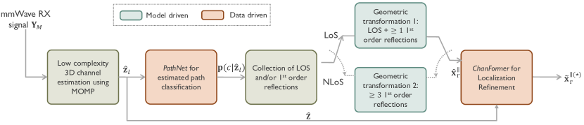
Figure 1: Diagram of the joint initial access and localization system model.

III-A MOMP-based channel estimation

Conventional compressive channel estimation methods exploit a representation of the received signal based on a dictionary obtained as Kronecker products of the dictionaries for the DoA, DoD, and delay domains. However, in our proposed 3D scenario, using the method will cause a prohibitive computational complexity that modern computers cannot handle. To address the issue, we exploit a sparse representation of the received signal in terms of a product of independent dictionaries instead of a Kronecker product based on MOMP, solving the sparse recovery problems by finding the support of the sparse representation of the channel. Let ${\bf Y}_{M}\in\mathbb{C}^{N_{\rm q}\times N_{{\mathrm{o}}}}$ be the observation, $\{{\bf\Psi}_{k}\in\mathbb{C}^{N_{k}^{\rm s}\times N_{k}^{\rm a}}\ |\ k=1,...,N_{{\mathrm{D}}}\}$ be a collection of $N_{\rm D}$ sparsifying dictionaries, and ${\bf\Phi}\in\mathbb{C}^{N_{\rm q}\times\otimes_{k=1}^{N_{\rm D}}N_{k}^{\rm s}}$ be the measurement tensor, then the sparse coefficients could be extracted from the tensor ${\bf C}\in\mathbb{C}^{\otimes_{k=1}^{N_{\rm D}}N_{k}^{\rm s}\times N_{\rm o}}$ by solving the optimization problem:

$$\min_{\bf C}\left(\left\|{\bf Y}_{M}-\sum_{{\bf i}\in\mathcal{I}}\sum_{{\bf j}\in\mathcal{J}}[{\bf\Phi}]_{:,{\bf i}}\left(\prod_{k=1}^{N_{\rm D}}[{\bf\Psi}_{k}]_{i_{k},j_{k}}\right)[{\bf C}]_{{\bf j},:}\right\|^{2}_{{\mathrm{F}}}\right),$$ (7)

where $\mathcal{I}=\{{\bf i}=(i_{1},\ldots,i_{N_{\rm D}})\in\mathbb{N}^{N_{\rm D}}|i_{k}\leq N_{k}^{\rm s},\ \forall k\leq N_{\rm D}\}$, and $\mathcal{J}=\{{\bf j}=(j_{1},\ldots,j_{N_{\rm D}})\in\mathbb{N}^{N_{\rm D}}|j_{d}\leq N_{k}^{\rm a},\ \forall k\leq N_{\rm D}\}$. Intuitively, the fundamental idea of the MOMP method is to rearrange elements into $N_{{\mathrm{D}}}$ orthogonal dimensions and execute tensor multiplications independently along each dimension for large-scale tensors, which yields the same results as using Kronecker product while freeing up more memories to accommodate larger tensor sizes.

The case of $N_{{\mathrm{D}}}=5$ independent dictionaries (for the azimuth and elevation DoA/DoD, and the time domain) is studied in [24], estimating the parameters in the $5$ dimensions simultaneously. For our case, however, to further reduce memory requirements targeting the outdoor localization problem that considers even greater arrays and incredibly fine resolutions, we focus on 1) estimating delays, DoDs, and the equivalent gains that include the effect of the path complex gains and the DoAs ($N_{{\mathrm{D}}}=3$), then 2) retrieving the DoAs from the equivalent gains. Let ${\bm{\Phi}}_{m_{{\mathrm{r}}},m_{{\mathrm{t}}}}\in\mathbb{C}^{Q\times N_{{\mathrm{t}}}^{{\mathrm{x}}}\times N_{{\mathrm{t}}}^{{\mathrm{y}}}\times N_{{\mathrm{d}}}}$ be the measurement tensor obtained with ${\mathbf{F}}_{m_{{\mathrm{t}}}}$ and ${\mathbf{W}}_{m_{{\mathrm{r}}}}$, the whole measurement tensor composed of ${\bm{\Phi}}_{m_{{\mathrm{r}}},m_{{\mathrm{t}}}}$ is ${\bm{\Phi}}\in\mathbb{C}^{QM_{{\mathrm{t}}}\times N_{{\mathrm{t}}}^{{\mathrm{x}}}\times N_{{\mathrm{t}}}^{{\mathrm{y}}}\times N_{{\mathrm{d}}}}$, and $[{\bf\Phi}]_{Q(m_{{\mathrm{t}}}-1)+q,{\bf i}}=[{\bf F}_{m_{{\mathrm{t}}}}{\bf s}[q-i_{3}]]_{i_{1}N_{{\mathrm{t}}}^{\rm x}+i_{2}}$. Three independent dictionaries are constructed:

$$\begin{cases}{\bf\Psi}_{1}=[\bar{\bf a}_{{\mathrm{t}}}^{\rm x}(\ddot{\phi}_{1}^{\rm x}),\cdots,\bar{\bf a}_{{\mathrm{t}}}^{\rm x}(\ddot{\phi}_{N_{1}^{\rm a}}^{\rm x})]\\ {\bf\Psi}_{2}=[\bar{\bf a}_{{\mathrm{t}}}^{\rm y}(\ddot{\phi}_{1}^{\rm y}),\cdots,\bar{\bf a}_{{\mathrm{t}}}^{\rm y}(\ddot{\phi}_{N_{2}^{\rm a}}^{\rm y})]\\ {\bf\Psi}_{3}=[{{\mathbf{p}}}_{{\mathrm{d}}}(\ddot{t}_{1}),\cdots,{{\mathbf{p}}_{{\mathrm{d}}}}(\ddot{t}_{N_{3}^{\rm a}})]\end{cases},$$ (8)

where ${\bf\Psi}_{1}$ and ${\bf\Psi}_{2}$ are for the discretized azimuth and elevation departure angular domains $\{\ddot{\phi}_{1}^{\rm x},\ldots,\ddot{\phi}_{N_{1}^{\rm a}}^{\rm x}\}$ and $\{\ddot{\phi}_{1}^{\rm y},\ldots,\ddot{\phi}_{N_{2}^{\rm a}}^{\rm y}\}$, and ${\bf\Psi}_{3}$ is for the discretized delay domain $\{\ddot{t}_{1},\ldots,\ddot{t}_{N_{3}^{\rm a}}\}$, where $[{\mathbf{p}}_{{\mathrm{d}}}(\ddot{t})]_{n}=f_{{\mathrm{p}}}\left((n-1)T_{s}-\ddot{t}\right)$. The effect of combiners and the arrival angular information are inside the equivalent gain tensor ${\bf C}\in\mathbb{C}^{N_{\rm 1}^{{\mathrm{a}}}\times N_{\rm 2}^{{\mathrm{a}}}\times N_{\rm 3}^{{\mathrm{a}}}\times N_{s}M_{{\mathrm{r}}}}$ which is sparse:

$$[{\bf C}]_{{\bf j},:}=\left\{\begin{array}[]{cl}{\bm{\beta}}_{\ell}^{{\sf T}}&\text{if }\begin{array}[]{c}\phi_{\ell}^{\rm x}=\ddot{\phi}_{j_{1}}^{\rm x},\phi_{\ell}^{\rm y}=\ddot{\phi}_{j_{2}}^{\rm y},\\ t_{\ell}-t_{0}=\ddot{t}_{j_{3}}\end{array};\\ 0&\text{o.w.}\end{array}\right..$$ (9)

where $[{\bm{\beta}}_{\ell}]_{N_{s}(m_{{\mathrm{r}}}-1)+n_{s}}=\alpha_{\ell}[{\bf W}_{m_{{\mathrm{r}}}}]^{*}_{:,n_{s}}{\bf a}_{{\mathrm{r}}}({\bm{\theta}}_{\ell})$. Now the components of Equ. (7) are ready, where ${\mathbf{Y}}_{M}$ is formed by collecting multiple observations using different pairs of ${\mathbf{F}}_{m_{{\mathrm{t}}}}$ and ${\mathbf{W}}_{m_{{\mathrm{r}}}}$:

$${\mathbf{Y}}_{M}=\left[\begin{array}[]{ccc}\breve{\bf Y}_{1,1}&\cdots&\breve{\bf Y}_{M_{{\mathrm{r}}},1}\\ \vdots&\ddots&\vdots\\ \breve{\bf Y}_{1,M_{{\mathrm{t}}}}&\cdots&\breve{\bf Y}_{M_{{\mathrm{r}}},M_{{\mathrm{t}}}}\\ \end{array}\right]\in\mathbb{C}^{QM_{{\mathrm{t}}}\times N_{s}M_{{\mathrm{r}}}}.$$ (13)

To retrieve the DoA information from the non-zero coefficients of ${\bf C}$ corresponding to the multipath components, the main idea is to correlate the coefficients with angular dictionaries and the DoAs could be determined by where the peaks exist. Let ${{\mathbf{W}}}_{M}=[\breve{{\mathbf{W}}}_{1},\cdots,\breve{{\mathbf{W}}}_{M_{{\mathrm{r}}}}]$, and here we remove the notations for measurement indices for simplicity, ${\bm{\beta}}_{\ell}$ can be rewritten as ${\bm{\beta}}_{\ell}=\alpha_{\ell}{{\mathbf{W}}}_{M}^{*}{{\mathbf{a}}}_{{\mathrm{r}}}({\bm{\theta}}_{\ell})$. Hence, assuming every entry of ${{\mathbf{W}}}_{M}$ is orthonormal, multiplying $\bm{\beta}_{\ell}^{*}$ to ${\bf W}_{M}^{*}$ and the angular dictionary gives:

$${\bm{\beta}}_{\ell}^{*}{{\mathbf{W}}}_{M}^{*}{\bf\Psi}_{{\mathrm{r}}}=\alpha_{\ell}{{\mathbf{a}}}_{{\mathrm{r}}}({\bm{\theta}}_{\ell})^{*}{{\mathbf{W}}_{M}{\mathbf{W}}^{*}_{M}}{\bf\Psi}_{{\mathrm{r}}}=\alpha_{\ell}{\mathbf{a}}({\bm{\theta}}_{\ell})^{*}{\bf\Psi}_{{\mathrm{r}}},$$ (14)

where ${\bf\Psi}_{{\mathrm{r}}}=[{{\mathbf{a}}}({\ddot{\bm{\theta}}}_{1}),...,{{\mathbf{a}}}({\ddot{\bm{\theta}}}_{N^{{\mathrm{a}}}_{4,5}})]$ is the arrival angular dictionary, which can be constructed as $\bm{\Psi}_{{\mathrm{r}}}=\bm{\Psi}_{4}\otimes\bm{\Psi}_{5}$, where $\bm{\Psi}_{4}$ and $\bm{\Psi}_{5}$ are similar to $\bm{\Psi}_{1}$ and $\bm{\Psi}_{2}$ in Equ. (8). The DoAs could be thus retrieved referring to the correlation peaks as:

$$\hat{\bm{\theta}}_{\ell}=\arg\max_{\ddot{\bm{\theta}}}\hat{\bm{\beta}}_{\ell}^{*}{\bf W}_{M}^{*}{\bf\Psi}_{{\mathrm{r}}}.$$ (15)

Equ. (15) can also be solved using MOMP by independent tensor multiplications in the azimuth and elevation arrival angular domain, especially when $N_{4}^{{\mathrm{s}}}\ (N_{5}^{{\mathrm{s}}})$ is large and high resolutions are needed. The computational complexity of our channel estimation algorithm is:

$$\mathcal{O}( N_{\rm est}(QM_{{\mathrm{t}}}+N_{s}M_{{\mathrm{r}}})(\sum_{k=1}^{3}N_{k}^{{\mathrm{a}}}N_{k}^{{\mathrm{s}}})$$ (16)

$$+N_{\rm est}N_{s}M_{{\mathrm{r}}}(N_{4}^{{\mathrm{a}}}N_{4}^{{\mathrm{s}}}+N_{5}^{{\mathrm{a}}}N_{5}^{{\mathrm{s}}})),$$

which is significantly lower than that of using the original OMP algorithm, which is $\mathcal{O}(N_{\rm est}(QM_{{\mathrm{t}}}+N_{s}M_{{\mathrm{r}}})(\prod_{k=1}^{5}N_{k}^{{\mathrm{a}}}N_{k}^{{\mathrm{s}}}))$ and modern computers cannot handle for our 3D settings.

The channel parameters required for localization – 3D DoDs/DoAs and TDoAs – are now available, except the path order which determines whether to discard an estimated path or not, as only LOS and 1st order reflections are usable in our system. The path classification problem is addressed in Sec. III-B.

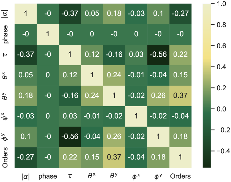
Figure 2: Correlation between each two of the channel parameters.

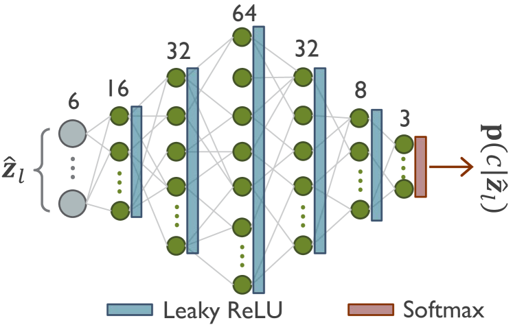
Figure 3: Architecture of PathNet.

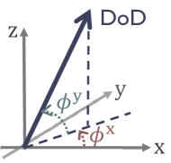
(a)

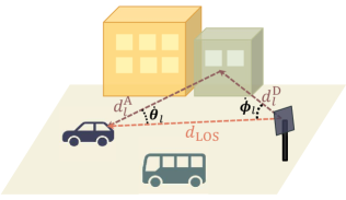
(b)

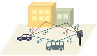
(c)

Figure 4: (a) Illustration of DoD, of which the unitary vector ${\bm{\phi}}=[\cos\phi^{{\mathrm{y}}}\cos\phi^{{\mathrm{x}}},\cos\phi^{{\mathrm{y}}}\sin\phi^{{\mathrm{x}}},\sin\phi^{{\mathrm{y}}}]^{{\sf T}}$; (b) LOS+NLOS localization; (c) NLOS-only localization.

III-B PathNet for path classification

The geometric relationships regarding LOS or NLOS channels can be exploited as shown in Fig. 4 for vehicle localizations. We consider the LOS path and/or a sufficient number of 1st order reflections necessary for our scheme, and higher order paths should be discarded. It is difficult to describe the relationship between the path order and the path parameters using a well-formulated model, thus we employ a data-driven approach based on DL to learn the relationship. To build a reasonable network, the correlations between the channel parameters and the path order are studied. As shown in Fig. 2, the path gain $|\alpha|$, TDoA $\tau$, azimuth and elevation DoAs/DoDs $\theta^{{\mathrm{x}}}$, $\theta^{{\mathrm{y}}}$, $\phi^{{\mathrm{x}}}$, $\phi^{{\mathrm{y}}}$ contribute to the path order, except the phase. Therefore, we decide the input of the network to be the normalized version of these parameters, denoted as ${\mathbf{z}}=[|\alpha|^{2},\tau,\theta^{{\mathrm{x}}},\theta^{{\mathrm{y}}},\phi^{{\mathrm{x}}},\phi^{{\mathrm{y}}}]$. Every estimated path $\hat{{\mathbf{z}}}_{\ell}$ must fall into one of the three categories: LOS ($c=1$), 1st order reflections ($c=2$), or others ($c=3$), given the probability vector output from PathNet, which is defined as:

$${\mathbf{p}}(c|\hat{{\mathbf{z}}})=\mathcal{F}(|\alpha|^{2},\tau,\theta^{{\mathrm{x}}},\theta^{{\mathrm{y}}},\phi^{{\mathrm{x}}},\phi^{{\mathrm{y}}};{\bm{\mu}}),$$ (17)

where $[{\mathbf{p}}(c|\hat{{\mathbf{z}}})]_{i}=p(c=i|\hat{{\mathbf{z}}},i\in\{1,2,3\})$, $\mathcal{F}(\cdot)$ represents the operations performed by PathNet, and ${\bm{\mu}}$ represents the network parameters to be trained. Hence, among $N_{\rm est}$ estimated paths of a channel, the LOS and 1st order reflections can be identified according to:

$$\hat{c}(\hat{{\mathbf{z}}})=\arg\max\limits_{i\in\{1,2,3\}}p(c=i|\hat{{\mathbf{z}}}).$$ (18)

As the input parameters are not like images with visible local features or like NLP problems that are usually context-sensitive and involving historical information, we simply adopt FC layers as the major components of the network, as it is usually a cheap way of learning non-linear combinations of features embedded in the input. The proposed architecture is shown in Fig. 3. To select an effective loss function to train the network, we notice that more penalties need to be applied when classifying the higher order as LOS/1st order reflections, which ruins the localization derivations, whereas less penalties make sense when the opposite happens because there are times when it is even advantageous to remove the LOS/1st order reflections with the features closer to those of higher order reflections, which may indicate inaccurate channel estimates. As such, a weighted cross entropy loss instead of a regular cross-entropy loss is adopted to adjust the penalties:

$$\mathcal{L}({\bm{\mu}})=-e^{-\eta(c({\bf z})-\hat{c}({\bf z}))}\cdot[{\mathbf{p}}(c|{\mathbf{z}})]_{c({\mathbf{z}})},$$ (19)

where $\eta$ is the customized weight coefficient.

III-C Localization via geometric transformations

Assuming imperfect synchronization between the vehicle and BS, and the clock offset to be $t_{0}$, two geometric transformations depending on the channel state are presented in Fig. 4b and 4c.

LOS+NLOS: Taking the example of LOS and a single 1st reflection ($l=1$) for the LOS+NLOS case as shown in Fig. 4b, the angle between the DoAs of the two paths is defined as $\dot{\theta}=\arccos({\bm{\theta}}_{\rm LOS}^{{\sf T}}{\bm{\theta}}_{\ell})$, and similarly $\dot{\phi}_{\ell}=\arccos({\bm{\phi}}_{\rm LOS}^{{\sf T}}{\bm{\phi}}_{\ell})$ represents the angle between the DoDs. The geometric transformation of the paths based on the law of sines can be acquired as:

$$\frac{d_{\rm LOS}}{\sin(\dot{\theta}_{\ell}+\dot{\phi}_{\ell})}=\frac{d_{\ell}^{\rm D}}{\sin(\dot{\theta}_{\ell})}=\frac{d_{\ell}^{\rm A}}{\sin(\dot{\phi}_{\ell})},$$ (20)

where $d_{\rm LOS}=||{\rm{\mathbf{x}}}_{{\mathrm{t}}}-{\rm{\mathbf{x}}}_{{\mathrm{r}}}||$ is the straight line distance between the 3D positions of the TX ${\rm{\mathbf{x}}}_{{\mathrm{t}}}$ and RX ${\rm{\mathbf{x}}}_{{\mathrm{r}}}$, which can be calculated by $d_{\rm LOS}=v_{{\mathrm{c}}}t_{\rm LOS}$, where $v_{{\mathrm{c}}}$ is the light speed and $t_{\rm LOS}$ is the time light travels; $d_{\ell}^{\rm D}$ ($d_{\ell}^{\rm A}$) is the distance between the TX (RX) and the interaction point on any surface, so that $d_{\ell}^{\rm D}+d_{\ell}^{\rm A}=v_{{\mathrm{c}}}t_{\ell}$. Hereby we have:

$$d_{\ell}^{{\mathrm{D}}}+d_{\ell}^{{\mathrm{A}}}-d_{\rm LOS}=v_{{\mathrm{c}}}(t_{\ell}-t_{\rm LOS})=v_{{\mathrm{c}}}\tau_{\ell},$$ (21)

where $\tau_{\ell}$ is the TDoA between the 1st reflection $l$ and the LOS. Combining Equ. (20) and (21), $d_{\rm LOS}$ can be derived as:

$$\hat{d}_{\rm LOS}=\frac{v_{{\mathrm{c}}}\tau_{\ell}\sin(\dot{\theta}_{\ell}+\dot{\phi}_{\ell})}{\sin(\dot{\theta}_{\ell})+\sin(\dot{\phi}_{\ell})-\sin(\dot{\theta}_{\ell}+\dot{\phi}_{\ell})}.$$ (22)

When the number of estimated 1st order reflections $L_{c=2}\geq 1$, $\hat{d}_{\rm LOS}$ can be obtained by solving the LS estimation problem:

$$\hat{d}_{\rm LOS}=\frac{<v_{{\mathrm{c}}}\cdot{{\rm{\bm{\tau}}}}\odot\sin(\dot{\bm{\theta}}+\dot{\bm{\phi}}),\sin(\dot{\bm{\theta}})+\sin(\dot{\bm{\phi}})-\sin(\dot{\bm{\theta}}+\dot{\bm{\phi}})>}{\|\sin(\dot{\bm{\theta}})+\sin(\dot{\bm{\phi}})-\sin(\dot{\bm{\theta}}+\dot{\bm{\phi}})\|^{2}},$$ (23)

where ${\bm{\tau}}=[\tau_{1},...,\tau_{L_{c=2}}]^{{\sf T}}$, $\dot{\bm{\theta}}=[\dot{\theta}_{1},...,\dot{\theta}_{L_{c=2}}]^{{\sf T}}$, and $\dot{\bm{\phi}}=[\dot{\phi}_{1},...,\dot{\phi}_{L_{c=2}}]^{{\sf T}}$. Finally, the vehicle location could be determined by:

$$\hat{\rm{\mathbf{x}}}_{{\mathrm{r}}}={\rm{\mathbf{x}}}_{{\mathrm{t}}}+\hat{d}_{\rm LOS}\cdot{\bm{\phi}}_{\rm LOS}.$$ (24)

NLOS-Only: As shown in Fig. 4c, the geometric transformation for path $l$ could be formed with an extension of Equ. (21):

$$\begin{cases}{\bf x}_{{\mathrm{r}}}+{\bm{\theta}}_{\ell}d_{\ell}^{{\mathrm{A}}}={{\mathbf{x}}}_{{\mathrm{t}}}+{\bm{\phi}}_{\ell}d_{\ell}^{{\mathrm{D}}}\\ d_{\ell}^{\rm A}+d_{\ell}^{{\mathrm{D}}}=\Delta d_{\ell}+d_{0}\end{cases},$$ (25)

where $\Delta d_{\ell}=v_{{\mathrm{c}}}(t_{\ell}-t_{0})$, and $d_{0}=v_{{\mathrm{c}}}t_{0}$. The vehicle location can be rewritten as:

$${\mathbf{x}}_{{\mathrm{r}}}={\mathbf{x}}_{{\mathrm{t}}}+({\bm{\phi}}_{\ell}+{\bm{\theta}}_{\ell})d_{\ell}^{{\mathrm{D}}}-{\bm{\theta}}_{\ell}(\Delta d_{\ell}+d_{0}),$$ (26)

and $d_{\ell}^{{\mathrm{D}}}$ is estimated as:

$$\hat{d}_{\ell}^{{\mathrm{D}}}=\frac{<{\bm{\phi}}_{\ell}+{\bm{\theta}}_{\ell},{\mathbf{x}}_{{\mathrm{r}}}-{\mathbf{x}}_{{\mathrm{t}}}+{\bm{\theta}}_{\ell}(\Delta d_{\ell}+d_{0})>}{||{\bm{\phi}}_{\ell}+{\bm{\theta}}_{\ell}||^{2}}.$$ (27)

Substitute $d_{\ell}^{{\mathrm{D}}}$ in Equ. (26) with the expression in Equ. (27), and let $\Theta_{\ell}=\frac{({\bm{\theta}}_{\ell}+{\bm{\phi}}_{\ell})({\bm{\theta}}_{\ell}+{\bm{\phi}}_{\ell})^{{\sf T}}}{||{\bm{\theta}}_{\ell}+{\bm{\phi}}_{\ell}||^{2}}$:

$${\mathbf{x}}_{{\mathrm{r}}}=({\mathbf{I}}-\Theta_{\ell}){\mathbf{x}}_{{\mathrm{t}}}+\Theta_{\ell}{\mathbf{x}}_{{\mathrm{r}}}-({\mathbf{I}}-\Theta_{\ell}){\bm{\theta}}_{\ell}(\Delta d_{\ell}+d_{0}),$$ (28)

which could be reduced to:

$$\begin{aligned} ({\mathbf{I}}-\Theta_{\ell})({\mathbf{x}}_{{\mathrm{r}}}+{\bm{\theta}}_{\ell}d_{0})=({\mathbf{I}}-\Theta_{\ell})[{\mathbf{I}},{\bm{\theta}}_{\ell}][{\mathbf{x}}_{{\mathrm{r}}};d_{0}]\\ =({\mathbf{I}}-\Theta_{\ell})({\mathbf{x}}_{{\mathrm{t}}}-{\bm{\theta}}_{\ell}\Delta d_{\ell})\end{aligned}.$$ (29)

The rank of $\Theta_{\ell}$ being $1$ makes the rank of $({\mathbf{I}}-\Theta_{\ell})$ to be $3-1=2$, and the rank of $[{\mathbf{I}},{\bm{\theta}}_{\ell}]$ is $3$, so the rank of $({\mathbf{I}}-\Theta)[{\mathbf{I}},{\bm{\theta}}_{\ell}]$ is $\min\{2,3\}=2$. When only a single 1st reflection is available, the solution set of Equ. (29) with $4$ unknowns – 3D vehicle position ${\mathbf{x}}_{{\mathrm{r}}}$ and the clock offset $t_{0}$ – has a dimension of $4-2=2$. Hence, there must be at least $3$ estimated 1st order reflections for the problem to have a unique solution of $[{\mathbf{x}}_{{\mathrm{r}}};d_{0}]$, which can be solved using LS estimation as:

$$[\hat{\bf x}_{{\mathrm{r}}};\hat{d}_{0}]={\bf A}^{-1}{\bf b},$$ (30)

for

$$\begin{cases}{\bf A}=\sum_{l=1}^{L_{c=2}}[{\mathbf{I}},{\bm{\theta}}_{\ell}]^{{\sf T}}({\mathbf{I}}-\Theta_{\ell})[{\mathbf{I}},{\bm{\theta}}_{\ell}]\\ {\bf b}=\sum_{l=1}^{L_{c=2}}[{\mathbf{I}},{\bm{\theta}}_{\ell}]^{{\sf T}}({\mathbf{I}}-\Theta_{\ell})({\bf x}_{{\mathrm{t}}}-{\bm{\theta}}_{\ell}\Delta d_{\ell})\end{cases}.$$

Once $\hat{\bf x}_{{\mathrm{r}}}$ is obtained, we can use the information to determine the location of the reflection points as well by inputting $\hat{\bf x}_{{\mathrm{r}}}$ into Equ. (25).

For both the LOS+NLOS and NLOS-only situations, multiple combinations of paths could exist to yield differing location estimates. In such a case, iterating over various combinations of paths and removing illogical localization results, e.g., those with unrealistic height estimations $\hat{x}_{{\mathrm{r}}}^{\perp}=[\hat{{\mathbf{x}}}_{{\mathrm{r}}}]_{3}$ (assuming height information is acquirable as downlink channel estimation is performed), can lead to satisfactory localization results. In the vehicular setting, we care particularly about the 2D location estimate $\hat{{\mathbf{x}}}_{{\mathrm{r}}}^{\shortparallel}=[\hat{{\mathbf{x}}}_{{\mathrm{r}}}]_{:2}$, which is the XY-plane location vector, for performance evaluations in the following sections.

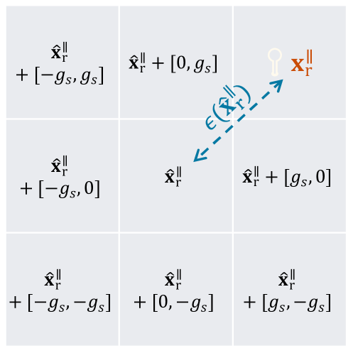
(a)

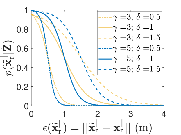
(b)

Figure 5: Illustration of (a) a $N_{g}\times N_{g}=3\times 3$ tile structure; (b) $p(\widetilde{{\mathbf{x}}}_{{\mathrm{r}}}^{\shortparallel}|\hat{{\mathbf{Z}}})$ vs. $\epsilon(\widetilde{{\mathbf{x}}}_{{\mathrm{r}}}^{\shortparallel})$ under various $\gamma$ and $\delta$ settings.

III-D ChanFormer for localization refinement

Noises may be introduced throughout the channel estimation and path classification process, and errors that accumulate and propagate will have a detrimental impact on the localization results. Modeling the noise is impractical as there are numerous influential factors, thus we turn to DL to approximate the mapping between the estimated paths and the true location. Instead of directly predicting the vehicle location from the received signal, where the localization accuracy is usually compromised in outdoor scenarios, we consider a $N_{g}\times N_{g}$ tile structure with a specified grid size $g_{s}$ around the initial 2D location estimate $\hat{{\mathbf{x}}}^{\shortparallel}_{{\mathrm{r}}}$, as an example shown in Fig. 5a, and create a network called ChanFormer that provides the probability of a tile containing the true location:

$$p\left(\widetilde{{\mathbf{x}}}_{{\mathrm{r}}}^{\shortparallel}|\hat{{\mathbf{Z}}}\right)=p\left({\mathbf{x}}_{{\mathrm{r}}}^{\shortparallel}=\widetilde{{\mathbf{x}}}_{{\mathrm{r}}}^{\shortparallel}|\hat{{\mathbf{Z}}},\widetilde{{\mathbf{x}}}_{{\mathrm{r}}}^{\shortparallel}=\hat{{\mathbf{x}}}^{\shortparallel}_{{\mathrm{r}}}+[n_{{\mathrm{x}}}g_{s},n_{{\mathrm{y}}}g_{s}]^{{\sf T}}\right),$$ (31)

where $\hat{{\mathbf{Z}}}=[\hat{{\mathbf{z}}}_{1};...;\hat{{\mathbf{z}}}_{N_{\rm est}}]$ is the estimated channel containing $N_{\rm est}$ estimated paths, and $|n_{{\mathrm{x}}}|,|n_{{\mathrm{y}}}|\in\left\{0,1,...,\frac{N_{g}-1}{2}\right\}$. $p(\widetilde{{\mathbf{x}}}_{{\mathrm{r}}}^{\shortparallel}|\hat{{\mathbf{Z}}})$ should be negatively related to the distance between $\widetilde{{\mathbf{x}}}_{{\mathrm{r}}}^{\shortparallel}$ and ${\mathbf{x}}_{{\mathrm{r}}}^{\shortparallel}$, which is formulated as :

$$p\left(\widetilde{{\mathbf{x}}}_{{\mathrm{r}}}^{\shortparallel}|\hat{{\mathbf{Z}}}\right)=\frac{1}{1+e^{-\gamma\left(1-\frac{||\widetilde{{\mathbf{x}}}_{{\mathrm{r}}}^{\shortparallel}-{\mathbf{x}}_{{\mathrm{r}}}^{\shortparallel}||}{\delta}\right)}},$$ (32)

where $\gamma$ is the belief factor, and $\delta$ is the scale factor for the distance $\epsilon(\widetilde{{\mathbf{x}}}_{{\mathrm{r}}}^{\shortparallel})=||\widetilde{{\mathbf{x}}}_{{\mathrm{r}}}^{\shortparallel}-{\mathbf{x}}_{{\mathrm{r}}}^{\shortparallel}||$. An illustration of the effects of $\gamma$ and $\delta$ can be found in Fig. 5b. ChanFormer is meant to analyze $\hat{{\mathbf{x}}}^{\shortparallel}_{{\mathrm{r}}}$ and its surroundings $\widetilde{{\mathbf{x}}}_{{\mathrm{r}}}^{\shortparallel}$ to find the one that most likely meets the current estimated channel condition, i.e., $\max_{\widetilde{{\mathbf{x}}}_{{\mathrm{r}}}^{\shortparallel}}p(\hat{{\mathbf{Z}}}|\widetilde{{\mathbf{x}}}_{{\mathrm{r}}}^{\shortparallel})$. The entire network can be formulated as:

$$\hat{{\mathbf{P}}}\left(\hat{{\mathbf{Z}}},\hat{{\mathbf{x}}}_{{\mathrm{r}}}^{\shortparallel}\right)=\mathcal{T}\left(\hat{{\mathbf{Z}}},\hat{{\mathbf{x}}}_{{\mathrm{r}}}^{\shortparallel};{\bm{\omega}}\right)\in\mathbb{R}^{1\times N_{g}^{2}},$$ (33)

where $\bm{\omega}$ is the network parameters to be trained. Inspired by the idea of the original Transformer [27], the core concept of ChanFormer is an encoder for Self-Attention to extract features of the input estimated channel $\hat{{\mathbf{Z}}}$, and a decoder to analyze the relationships between the estimated channel features and the initial location estimate $\hat{{\mathbf{x}}}_{{\mathrm{r}}}^{\shortparallel}$ using Encoder-Decoder Attention. The proposed architecture is shown in Fig. 6.

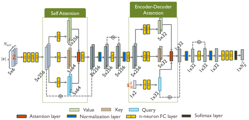
Figure 6: Architecture of ChanFormer. The self-attention block extracts the intra and crossover features of the input estimated paths; The encoder-decoder block analyzes the relationship between the initial location estimate and the extracted features of the estimated paths.

Encoder: The workflow starts with FC layers embedding the input estimated paths to vectors with a length of $256$. Then, the self-attention process begins by creating three abstraction matrices – query, key, and value matrices, denoted as ${\mathbf{Q}}$, ${\mathbf{K}}$, and ${\mathbf{V}}$ respectively, where each row of the matrices corresponds to an estimated path. Conceptually, each $\hat{{\mathbf{z}}}_{\ell}$ now has a high-dimensional interpretation of its features in its value $[{\mathbf{V}}]_{l,:}$, which can be indexed by its key $[{\mathbf{K}}]_{l,:}$. The following attention layer then evaluates the relationships among the paths by:

$${\rm Attention}({\mathbf{Q}},{\mathbf{K}},{\mathbf{V}})={\rm softmax}\left(\frac{{\mathbf{Q}}{\mathbf{K}}^{{\sf T}}}{\sqrt{d_{{\mathrm{k}}}}}\right){\mathbf{V}},$$ (34)

where $d_{{\mathrm{k}}}$ is the dimension of $[{\mathbf{K}}]_{l,:}$, and $\rm softmax$ is for atoms along $\rm axis=2$. The softmax score determines how much true channel information is represented by the $l$-th estimated path by examining the correlation between $\hat{{\mathbf{z}}}_{\ell}$ and all the paths in $\hat{{\mathbf{Z}}}$. It is expected that $\hat{{\mathbf{z}}}_{l}$ will have the highest softmax score with itself, but other paths that have quite accurate estimations will also be assigned a relatively high score. Therefore, the $\rm Attention$ output is the expression of each path that integrates information from all other paths. The less reliable estimated paths will have a smaller influence on the expressions. Simply put, this means that the attention mechanism places more emphasis on the more accurate paths in this step, so that the true channel is better represented, regardless of the presence of the noises from the channel estimation process and/or the misclassified paths. In addition, the attention layer is capable of analyzing the input without being constrained by its chronicle orders, which exceeds the capabilities of the convolutional layer that considers path relationships within a fixed window, or the FC layer that relies on connections of all the input parameters.

Decoder: The input $\hat{{\mathbf{x}}}_{{\mathrm{r}}}^{\shortparallel}$ serves as a query, referring to which the network generates the probability map ${\mathbf{P}}(\hat{{\mathbf{Z}}})^{\star}\in\mathbb{R}^{N_{g}\times N_{g}}$ of the tiles with $\hat{{\mathbf{x}}}_{{\mathrm{r}}}^{\shortparallel}$ at the center. Note that, though $\hat{{\mathbf{x}}}_{{\mathrm{r}}}^{\shortparallel}$ is the only input at the decoder, the network actually takes all the candidate locations in the tiles into consideration. In this part, the attention layer improves the initial location estimate accuracy by assigning a higher probability to a candidate location $\widetilde{{\mathbf{x}}}_{{\mathrm{r}}}^{\shortparallel}$ that aligns better with the channel representation obtained from the encoder. Note that the output $\hat{{\mathbf{P}}}(\hat{{\mathbf{Z}}},\hat{{\mathbf{x}}}_{{\mathrm{r}}}^{\shortparallel})$ is reshaped to ${\mathbf{P}}(\hat{{\mathbf{Z}}},\hat{{\mathbf{x}}}_{{\mathrm{r}}}^{\shortparallel})^{\star}\in\mathbb{R}^{N_{g}\times N_{g}}$ to acquire the probability map to simplify the process of accessing $\widetilde{{\mathbf{x}}}_{{\mathrm{r}}}^{\shortparallel}$ associated with $p(\widetilde{{\mathbf{x}}}_{{\mathrm{r}}}^{\shortparallel}|\hat{{\mathbf{Z}}})$. By referring to the tile with the highest probability:

$$=\arg\max\limits_{j,i}\left[\hat{{\mathbf{P}}}(\hat{{\mathbf{Z}}},\hat{{\mathbf{x}}}_{{\mathrm{r}}}^{\shortparallel})^{\star}\right]_{j,i}\Rightarrow$$ (35)

$$[n_{{\mathrm{x}}}^{\star},n_{{\mathrm{y}}}^{\star}]=\left[i^{\star}-\frac{N_{g}+1}{2},\frac{N_{g}+1}{2}-j^{\star}\right],$$

the refined location is given by:

$$\widetilde{{\mathbf{x}}}_{{\mathrm{r}}}^{\shortparallel(\star)}=\hat{{\mathbf{x}}}^{\shortparallel}+[n_{{\mathrm{x}}}^{\star}g_{s},n_{{\mathrm{y}}}^{\star}g_{s}]^{{\sf T}}.$$ (36)

To train the network, MSE loss or the KL divergence loss to learn the probability map distribution could be used.

IV Simulation Results

In this section, we present simulation results to verify the concepts discussed in this work. We begin by detailing the simulation setups in Sec. IV-A. Then in Sec. IV-B, we implement the MOMP based channel estimation to establish a solid foundation for the subsequent tasks. In Sec. IV-C, we demonstrate the results of path classification using PathNet for the simulated channels, achieving $99\%$ classification accuracy. We then discuss the localization through geometric transformations using the estimated channel parameters and predicted path orders in Sec. IV-D, where we observe that the sub-meter accuracy is not achieved for a sufficient number of users. The localization refinement using ChanFormer is thus implemented in Sec. IV-E, which results in a considerable decrease in 2D localization errors, achieving the desired sub-meter localization.

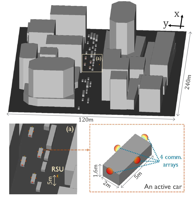
Figure 7: Ray-tracing simulation of an urban environment with cars and trucks distributed across $4$ lanes.

IV-A Simulation setups

Ray-tracing simulation for realistic channels: We run $2500$ electromagnetic simulations of a vehicular environment in Rosslyn City, Virginia, on a $240\times 120$ m² plane, using Wireless Insite software[28], as the snapshot shown in Fig. 7. In each simulation, around $30$ vehicles are randomly distributed across the four lanes for initial access, with $80\%$ being cars and $20\%$ being trucks according to the 3GPP vehicular communication requirement [25]. The RSU is located at ${\mathbf{x}}_{{\mathrm{t}}}=[120,-21,5]$ m, down facing the road. Parameters for materials of the building/territorial surfaces, the vehicle sizes, placements of antennas on the vehicle and RSU, etc., follow the deployments in [29]. $4$ active cars are randomly selected to communicate with the RSU in the $73$ GHz band. With each car equipped with $4$ communication arrays, the simulations provide $4\times 4\times 2500=40$k as the dataset $\mathcal{S}$, and every channel has $L=25$ multipath components. The first $24$k channels are split into $3:1$ for training and validations, denoted as $\mathcal{S}_{\rm tr}$ and $\mathcal{S}_{\rm val}$, and the remaining $16$k channels serve as the testing set $\mathcal{S}_{\rm te}$ for all the performance evaluations.

Communication system: Localization performance with various antenna settings and transmitted power levels are studied in [30]. In this paper, we use an antenna setting of $N_{{\mathrm{t}}}=N_{{\mathrm{t}}}^{{\mathrm{x}}}\times N_{{\mathrm{t}}}^{{\mathrm{y}}}=16\times 16$, $N_{{\mathrm{r}}}=N_{{\mathrm{r}}}^{{\mathrm{x}}}\times N_{{\mathrm{r}}}^{{\mathrm{y}}}=8\times 8$, and a transmitted power of $P_{{\mathrm{t}}}=40$ dBm for a better performance. The number of RF chains are set to be $N_{{\mathrm{t}}}^{\rm RF}=8$ and $N_{{\mathrm{r}}}^{\rm RF}=4$. The communication system operates at a carrier frequency $f_{c}=73$ GHz with a bandwidth $B_{c}=1$ GHz. $\sigma^{2}_{{\mathbf{n}}}=-84$ dBm is calculated accordingly using $T=288^{\degree}$F. Given the RMS delay-spread of the simulated channels and the bandwidth, the number of delay taps is fixed to $N_{{\mathrm{d}}}=64$. $N_{s}=\min\{N_{{\mathrm{t}}}^{\rm RF},N_{{\mathrm{r}}}^{\rm RF}\}=4$ training data streams with a length of $Q=64$ are transmitted. We use the raised-cosine filter with a roll-off factor of $0.4$ as the pulse shaping function.

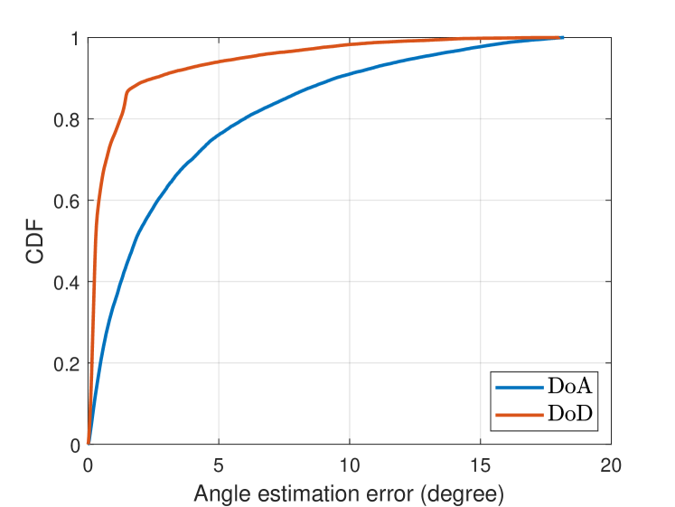
(a)

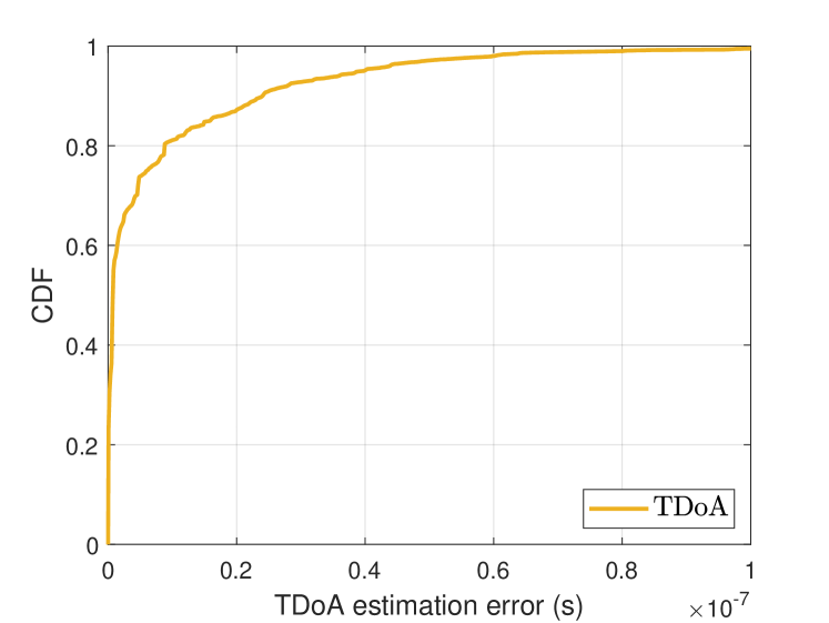
(b)

Figure 8: MOMP based channel estimation performance using a setting of a $16\times 16$ array at the TX and a $8\times 8$ array at the RX. Plots acquired based on the whole dataset $\mathcal{S}$.

IV-B MOMP based low complexity 3D channel estimation

The precoders ${\mathbf{F}}$ are constructed by the Khatri-Rao product of the precoders along the azimuth and elevation planes, i.e., ${\mathbf{F}}={\mathbf{F}}^{{\mathrm{x}}}\circ{\mathbf{F}}^{{\mathrm{y}}}$. Each column of ${\mathbf{F}}^{{\mathrm{x}}}$ (${\mathbf{F}}^{{\mathrm{y}}}$) is extracted from the DFT codebook of size $N_{{\mathrm{t}}}^{{\mathrm{x}}}$ ($N_{{\mathrm{t}}}^{{\mathrm{y}}}$), e.g., $\forall[{\mathbf{F}}^{{\mathrm{x}}}]_{:,i}\in\left\{{\mathbf{a}}^{\prime}(\varphi)|\varphi=0,\frac{2\pi\cdot 1}{N_{{\mathrm{t}}}^{{\mathrm{x}}}},...,\frac{2\pi\cdot(N_{{\mathrm{t}}}^{{\mathrm{x}}}-1)}{N_{{\mathrm{t}}}^{{\mathrm{x}}}}\right\}$, where ${\mathbf{a}}^{\prime}(\varphi)=\frac{1}{\sqrt{N_{{\mathrm{t}}}^{{\mathrm{x}}}}}\left[0,e^{j\cdot 1\cdot\varphi},...,e^{j\cdot(N_{{\mathrm{t}}}^{{\mathrm{x}}}-1)\cdot\varphi}\right]^{{\sf T}}$. The same rule applies to the combiners ${\mathbf{W}}$. We use a setting of $M_{{\mathrm{t}}}=16;\ M_{{\mathrm{r}}}=64$, and form ${\mathbf{Y}}_{M}$ by collecting a total of $M=M_{{\mathrm{r}}}\times M_{{\mathrm{t}}}=1024$ frames [31]. The size, or the resolution, of the dictionaries is based on the number of their atoms along the dimension, with a specific constant $K_{\rm res}$ determining the proportion, i.e., $N_{k}^{{\mathrm{a}}}=K_{\rm res}\cdot N_{k}^{{\mathrm{s}}}$. In our case, $N_{1}^{{\mathrm{s}}}=N_{{\mathrm{t}}}^{{\mathrm{x}}}$, $N_{2}^{{\mathrm{s}}}=N_{{\mathrm{t}}}^{{\mathrm{y}}}$, and $N_{3}^{{\mathrm{s}}}=N_{{\mathrm{d}}}$. The impact of $K_{\rm res}$ is studied in [24]. Here we set $K_{\rm res}=128$ as it brings a comparable performance to using a higher resolution setting, such as $K_{\rm res}=1024$, while being computationally more efficient.

The angle and delay estimation performance can be found in Fig. 8. The estimation errors are calculated by matching an estimated path to its closest true path in the channel. We obtain better DoD estimations angle errors of $\leq 10^{\degree}$ compared to DoA estimations which mostly have angle errors of $\leq 15^{\degree}$. This is reasonable as the TX is equipped with a $16\times 16$ antenna array, while the RX array size is $8\times 8$. A delay error of $\leq 5e-8$ s can be expected. The angle and delay estimates may not appear accurate enough for localization when all estimated paths, including those with large noises such as higher order reflections, are associated with true paths. However, this does not necessarily reflect the localization accuracy as PathNet will identify the usable paths.

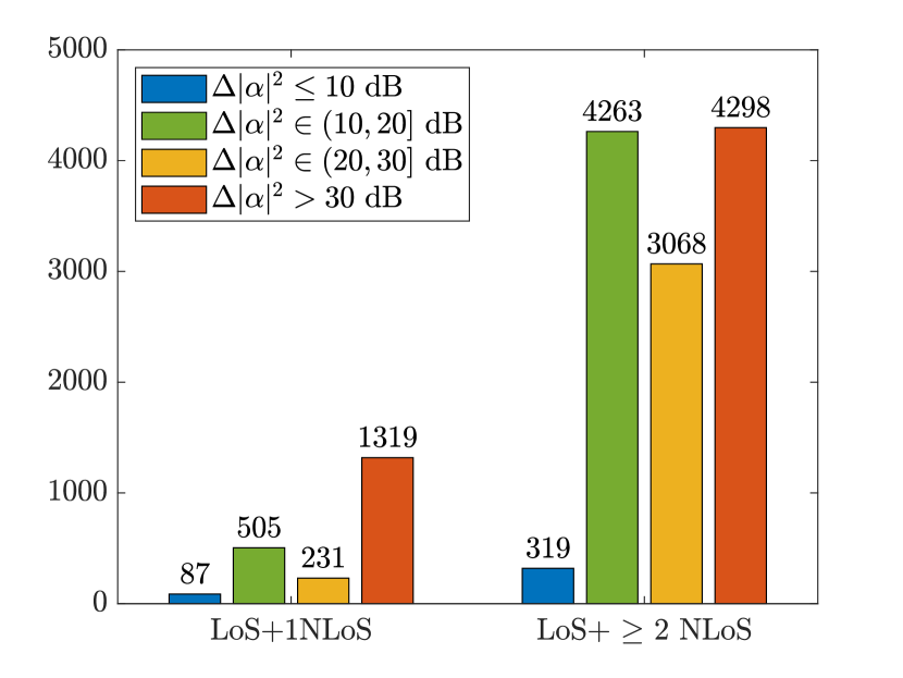
Figure 9: Distribution of the power gap $\Delta|\alpha|^{2}$ between the LOS and strongest 1st order path of $14$k valid LOS channels from the entire dataset containing $40$k channels. $40\%$ channels are with $\Delta|\alpha|^{2}>30$ dB.

IV-C PathNet for path classification

PathNet is trained based on $\mathcal{S}_{\rm tr}$ and $\mathcal{S}_{\rm val}$, which lasts for $1000$ epochs with an early stopping depending on the convergence of the validation loss. We adopt Adam optimizer [32], and set the learning rate $1e-3$ with a decay rate of $0.95$ every $200$ training epochs. The customized weight for tweaking the penalty in $\mathcal{L}({\bm{\mu}})$ is set to $\eta=0.2$. The path classification performance presented in Table I is evaluated using the channels in $\mathcal{S}_{\rm te}$ that the network has never seen, providing classification accuracies in the order of $99\%$ in a vehicular setting, which demonstrates the strong generalization ability of the proposed simple yet effective network.

Overall	LOS ($c=1$)	1st order path ($c=2$)	Other ($c=3$)
$98.81\%$	$99.86\%$	$99.13\%$	$98.67\%$

Table I: Categorical path classification accuracy based on $16$k testing channels ($25$ paths simulated for each channel).

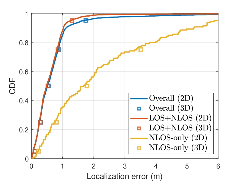
Figure 10: Localization performance using geometric transformations based on $2349$ qualified estimated channels ($2210$ LOS; $139$ NLOS) in $\mathcal{S}^{+}_{\rm te}$ (added 3D loc errors).

Channel	$5$th	$50$th	$80$th	$95$th
Overall	$0.06$	$0.51$	$0.92$	$1.70$
Overall⋆	$0.04$	$0.22$ $57\%\downarrow$	$0.32$ $65\%\downarrow$	$0.72$ $58\%\downarrow$
LOS+NLOS	$0.06$	$0.49$	$0.88$	$1.26$
LOS+NLOS⋆	$0.04$	$0.21$ $57\%\downarrow$	$0.31$ $65\%\downarrow$	$0.45$ $64\%\downarrow$
NLOS	$0.21$	$1.67$	$3.87$	$5.97$
NLOS⋆	$0.09$	$0.75$ $55\%\downarrow$	$3.63$	$5.80$

Table II: Percentile statistics of 2D localization errors (m) with and without ChanFormer. $\star$: location estimates refined by ChanFormer; “Overall” shows the merged localization results of using channels in $\mathcal{S}^{+}_{\rm te}$.

IV-D Localization based on geometric transformations

To acquire reasonable localization results, we first examine the entire database which contains $14$k valid LOS channels ($L_{c=2}\geq 1$) and $24$k valid NLOS channels ($L_{c=2}\geq 3$), and establish criteria to exclude channels indicating the vehicle being not locatable. For valid LOS channels, we measure the power gap $\Delta|\alpha|^{2}$ between the LOS and the strongest 1st order path, as shown in Fig. 9, $40\%$ of the channels are with $\Delta|\alpha|^{2}>30$ dB, so the 1st order reflections cannot be estimated accurately or even detected. For valid NLOS channels, we check the received power levels to determine a threshold to ensure reliable channel estimations. It is important to note that while these simulated realistic channels provide a useful representation of real-world channels, they do have limitations due to the absence of factors such as traffic lights and building windows that can produce additional reflections, some of which can be quite strong. These factors could have an impact on the overall channel characteristics. In our settings, we argue that a vehicle is locatable when the channel status satisfies the following rules: 1) The channel is valid with sufficient paths for localization; 2) $\Delta|\alpha|^{2}\leq 30$ dB for LOS channels; 3) For each NLOS-only channel, the set of 1st order reflections with a received power of $P_{{\mathrm{r}}}\geq-80$ dBm – $\mathcal{Z}=\left\{\hat{{\mathbf{z}}}_{\ell}\ |\ P_{{\mathrm{r}}}(l)\geq-80\ {\text{dBm}},c(\hat{{\mathbf{z}}}_{\ell})=2\right\}$ – has a length of $|\mathcal{Z}|\geq 3$. It is worth noticing that the statistic is based on ideal channels rather than the estimated, hence there are likely fewer estimated channels that qualify for usage in our localization strategy.

Considering real applications, the vehicle location is calculated based on the array with the strongest received power, thereby the dataset size is $4\times$ smaller. The new sets are denoted as $\mathcal{S}^{+}_{\rm tr}\in\mathcal{S}_{\rm tr}$, $\mathcal{S}^{+}_{\rm val}\in\mathcal{S}_{\rm val}$, and $\mathcal{S}^{+}_{\rm te}\in\mathcal{S}_{\rm te}$. There exist $2349$ qualified estimated channels ($2210$ LOS and $139$ NLOS) in $\mathcal{S}^{+}_{\rm te}$, based on which the localization performance is plotted in Fig. 10, showing the CDF of localization error (m). The 3D error distribution is close to the 2D one, because we have the height information which helps in identifying accurate location estimates. For the following evaluations, we will primarily focus on the 2D errors. The 5, 50, 80, 95th-percentile accuracies are presented in Table II. Hereby we claim that sub-meter accuracy localization is realized for $80\%$ of the users in LOS channels and $35\%$ of the users in NLOS channels. The performance is compromised for NLOS channels because of the small pool of qualified estimated paths and the decreased accuracy of channel estimations. Nevertheless, the performance we have achieved should be considered as the worst-case scenario, as the real-world channels are likely to include more reflections from traffic lights and building windows with higher power.

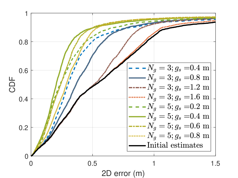
Figure 11: Overall 2D localization error (m) when training ChanFormer on $\mathcal{S}^{+}_{\rm tr}$ using various tile settings.

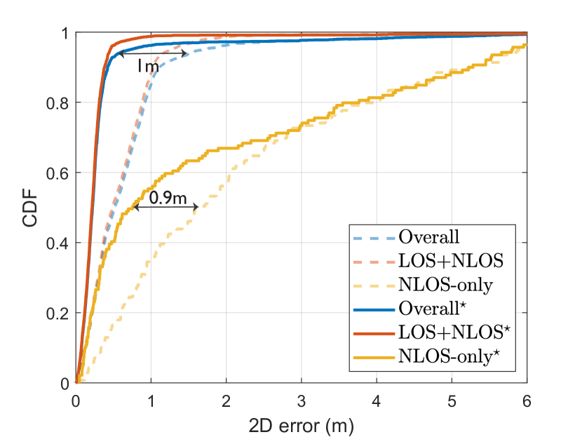
Figure 12: ChanFormer refined (with ^⋆) location estimates. The 95th-percentile 2D error is reduced by $1$ m ($58\%\downarrow$) overall. The error is $64\%\downarrow$ for $95\%$ of users in LOS channels, and $55\%\downarrow$ for $50\%$ of users in NLOS channels, realizing the expected sub-meter localization.

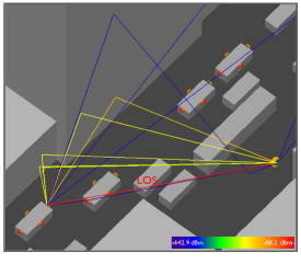
(a) LOS channel

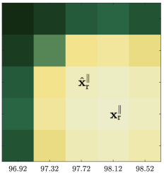
(b) True ${\mathbf{P}}(\hat{{\mathbf{Z}}},\hat{{\mathbf{x}}}_{{\mathrm{r}}}^{\shortparallel})$ (LOS)

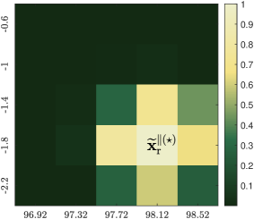
(c) Predicted ${\mathbf{P}}(\hat{{\mathbf{Z}}},\hat{{\mathbf{x}}}_{{\mathrm{r}}}^{\shortparallel})^{\star}$ (LOS)

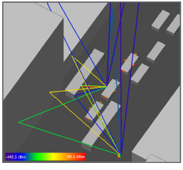
(d) NLOS channel

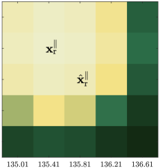
(e) True ${\mathbf{P}}(\hat{{\mathbf{Z}}},\hat{{\mathbf{x}}}_{{\mathrm{r}}}^{\shortparallel})$ (NLOS)

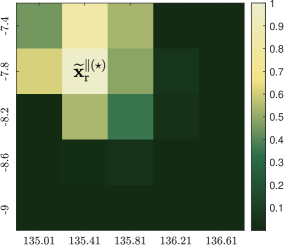
(f) Predicted${\mathbf{P}}(\hat{{\mathbf{Z}}},\hat{{\mathbf{x}}}_{{\mathrm{r}}}^{\shortparallel})^{\star}$ (NLOS)

Figure 13: An example of pairs of a ground truth and a ChanFormer predicted (with $\star$) probability map under LOS (a, b) / NLOS (c, d) conditions. (a, b) True location: $[98.07,-1.75]$; Initial error $0.50$ m; Error after refinement: $0.07$ m ($0.43$ m $\downarrow$). (c, d) True location: $[135.48,-7.75]$; Initial error: $0.56$ m; Error after refinement: $0.08$ m ($0.47$ m $\downarrow$). The examples are from $\mathcal{S}_{\rm te}^{+}$. (good examples of LOS and a NLOS cases)

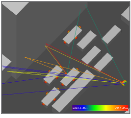
(a) NLOS channel

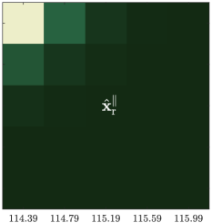
(b) True ${\mathbf{P}}(\hat{{\mathbf{Z}}},\hat{{\mathbf{x}}}_{{\mathrm{r}}}^{\shortparallel})$ (NLOS)

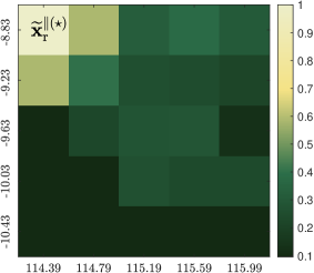
(c) Predicted ${\mathbf{P}}(\hat{{\mathbf{Z}}},\hat{{\mathbf{x}}}_{{\mathrm{r}}}^{\shortparallel})^{\star}$ (NLOS)

Figure 14: An example of a pair of true and predicted probability map when the initial estimate is far from the true location. ChanFormer pulls the initial estimate $[115.19,-9.63]$ towards the true location $[113.55,-7.75]$, providing an error reduction from $2.5$ m to $1.36$ m ($1.13$ m $\downarrow$). (added a situation beyond the network’s capability.)

IV-E ChanFormer for localization refinement

The impacts of $\gamma$ and $\delta$ are studied as shown in Fig. 5b, accordingly to which $\gamma=5$ and $\delta=1$ are set in Equ. (32) to have a smooth and balanced probability function. A $5\times 5$ tile structure with a grid size $g_{s}=0.4\text{ m}$ is adopted, which is found to be the best option among the settings shown in Fig. 11. ChanFormer is trained based on $3568$ qualified channels ($3316$ LOS / $252$ NLOS) in $\mathcal{S}^{+}_{\rm tr}$ and $\mathcal{S}^{+}_{\rm val}$, with a batch size of $32$. Adam optimizer is used, and the learning rate is $2e-4$ with a decay rate of $0.95$ per $200$ epochs. Loss on the validation set is monitored for early stopping.

The refined localization performance based on set $\mathcal{S^{+}_{\rm te}}$ can be found in Fig. 12, and the percentile statistics are shown in Table II. Overall, the 80, 95th-percentile accuracy is improved by $65\%$ and $58\%$. The refinement reduces the 95th-percentile 2D error to $0.45$ m from $1.26$ m, i.e., $64\%$ improvement in the accuracy, for users in the LOS, and an error reduction to $0.75$ m from $1.67$ m, i.e., $55\%$ accuracy improvement, is achieved for half of the users in the channel of NLOS. In conclusion, sub-meter localization is realized for $95\%$ of the users in LOS channels and $50\%$ of the users in the channel of NLOS. Fig. 13 shows an example of pairs of ground truth and predicted probability maps under LOS and NLOS situations for intuition. A reduction of 2D error from $\epsilon(\hat{{\mathbf{x}}}_{{\mathrm{r}}}^{\shortparallel})=0.5\text{ m}$ to $\epsilon(\widetilde{{\mathbf{x}}}_{{\mathrm{r}}}^{\shortparallel})=0.07$ m for the LOS case, and an error reduction from $0.56$ m to $0.08$ m for the NLOS case, are realized. Note that, ChanFormer working like a filter can be effective when the initial location estimate error $\epsilon(\hat{{\mathbf{x}}}_{{\mathrm{r}}}^{\shortparallel})<2.5$ m, allowing the network to remove the noise embedded in both $\hat{{\mathbf{Z}}}$ and $\hat{{\mathbf{x}}}_{{\mathrm{r}}}^{\shortparallel}$, and pull the location estimate in the right direction, whereas it cannot effectively correct $\epsilon(\hat{{\mathbf{x}}}_{{\mathrm{r}}}^{\shortparallel})$ when $\hat{{\mathbf{x}}}_{{\mathrm{r}}}^{\shortparallel}$ is hopped too far away from the tile panel, especially in the NLOS case. Fig. 14 illustrates the situation where ChanFormer enables an error reduction of $1.13$ m, but the error remains at $1.3$ m as the initial estimate is $2.5$ m away from the true location.

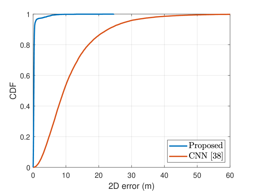
Figure 15: Comparison with the CNN method using power delay profiles in [23] (CDF based on $\mathcal{S}^{+}_{\rm te}$ following our experimental settings).

Most of the previous studies mentioned in Sec. I-A assume unrealistic artificially controlled channels and simplistic communication system settings, limiting their comparability to our methods. The comparable work [23] considers realistic channels in the area of New York University (NYU) and uses a CNN based architecture to map power delay profiles to the UE locations. We migrated their proposed algorithms to our simulation environment and set the number of partitions to $4$. The reproduced localization results with our experimental settings could be found in Fig. 15. Our model and data-driven localization method outperforms their work by achieving the sub-meter localization for $95\%$ of the users, while their $5$th, $50$th, $80$th, and $95$th percentile errors are $2.25$, $9.36$, $16.87$, and $28.59$ m, respectively.

V Conclusion and Future Work

We used a hybrid data/model driven method to realize 3D localization in the mmWave V2I network. We considered a realistic channel model that includes the filtering effects and an unknown TX-RX clock offset, and generated channel datasets using ray-tracing. We proposed to first remove the high order reflections – which are the majority of a realistic channel – using PathNet, which achieved a classification accuracy of $99\%$ that provided a solid foundation for the localization strategy. The model-driven 3D location estimator is then formulated through geometric transformations among the locations of the vehicle, scatters, and the RSU. The estimator worked in both LOS and NLOS scenarios, requiring sufficient 1st order reflections though. The estimator realized sub-meter accuracies for $80\%$ of users in LOS channels and for $35\%$ of users in NLOS channels. We treated the results to be less satisfactory, and thus designed the location refinement network ChanFormer, which found a better representation of an estimated channel and indicated the most probable vehicle location under the channel status. As a result, $95\%$ of users in the LOS channels can have a 2D localization accuracy of $0.45$ m, and $50\%$ of users in the NLOS channels can have an accuracy of $0.75$ m. Overall, the performance has been improved by $55\%\sim 65\%$ depending on the scenario. The results demonstrate that the idea of attention is well-suited to our scenario without any gaps, and also highlight the potential of migrating advanced DNN architectures to the field of wireless communications.

Current work is for initial access, where the NLOS-only situation could be a bit concerning regarding the achieved accuracy. Integrating other onboard sensors could be a solution for higher accuracy. In addition, this research will be extended to vehicle location tracking using mmWave RX signals or sensor fusion. With historical channel and location information, solutions for occasional blockages in a trajectory could be provided. Attention based methods could also be used, which could outperform traditional network architectures for time series processing, e.g., LSTM [33], which processes the inputs sequentially and can be still prone to losing important earlier information due to memory limitations. Furthermore, in highly dynamic scenarios, an alternative approach to consider is V2V sidelink assisted localization, which facilitates direct communication between vehicles without relying on connectivity through cellular infrastructures.

References

- [1] A. Shahmansoori, G. E. Garcia, G. Destino, G. Seco-Granados, and H. Wymeersch, “Position and orientation estimation through millimeter-wave MIMO in 5G systems,” IEEE Trans. on Wireless Commun/, vol. 17, no. 3, pp. 1822–1835, 2018.
- [2] T. Wild, V. Braun, and H. Viswanathan, “Joint design of communication and sensing for beyond 5g and 6g systems,” IEEE Access, vol. 9, pp. 30 845–30 857, 2021.
- [3] Q. Tao, Z. Hu, Z. Zhou, H. Xiao, and J. Zhang, “SeqPolar: Sequence matching of polarized lidar map with HMM for intelligent vehicle localization,” IEEE Transactions on Vehicular Technology, 2022.
- [4] K. Ćwian, M. R. Nowicki, and P. Skrzypczyński, “GNSS-augmented LiDAR SLAM for accurate vehicle localization in large scale urban environments,” in 2022 17th International Conference on Control, Automation, Robotics and Vision (ICARCV). IEEE, 2022, pp. 701–708.
- [5] M.-S. Kang, J.-H. Ahn, J.-U. Im, and J.-H. Won, “Lidar-and V2X-based cooperative localization technique for autonomous driving in a GNSS-denied environment,” Remote Sensing, vol. 14, no. 22, p. 5881, 2022.
- [6] A. Schaefer, D. Büscher, J. Vertens, L. Luft, and W. Burgard, “Long-term vehicle localization in urban environments based on pole landmarks extracted from 3-d lidar scans,” Robotics and Autonomous Systems, vol. 136, p. 103709, 2021.
- [7] V. Ilci and C. Toth, “High definition 3D map creation using GNSS/IMU/LiDAR sensor integration to support autonomous vehicle navigation,” Sensors, vol. 20, no. 3, p. 899, 2020.
- [8] Y. Liang, S. Müller, D. Schwendner, D. Rolle, D. Ganesch, and I. Schaffer, “A scalable framework for robust vehicle state estimation with a fusion of a low-cost IMU, the GNSS, radar, a camera and lidar,” in 2020 IEEE/RSJ International Conference on Intelligent Robots and Systems (IROS). IEEE, 2020, pp. 1661–1668.
- [9] R. Keating, A. Ghosh, B. Velgaard, D. Michalopoulos, and M. Säily, “The evolution of 5G New Radio positioning technologies,” Nokia Bell Labs, Tech. Rep., 02 2021.
- [10] X. Wu, G. Yang, F. Hou, and S. Ma, “Low-complexity downlink channel estimation for millimeter-wave FDD massive MIMO systems,” IEEE Wireless Communications Letters, 2019.
- [11] A. C. Gurbuz, Y. Yapici, and I. Guvenc, “Sparse channel estimation in millimeter-wave communications via parameter perturbed OMP,” in 2018 IEEE International Conference on Communications Workshops (ICC Workshops). IEEE, 2018, pp. 1–6.
- [12] A. Mejri, M. Hajjaj, and S. Hasnaoui, “Structured analysis/synthesis compressive sensing-based channel estimation in wideband mmWave large-scale multiple input multiple output systems,” Transactions on Emerging Telecommunications Technologies, vol. 31, no. 7, p. e3903, 2020.
- [13] J. Rodríguez-Fernández, N. González-Prelcic, K. Venugopal, and R. W. Heath, “Frequency-domain compressive channel estimation for frequency-selective hybrid millimeter wave MIMO systems,” IEEE Trans. on Wireless Commun., vol. 17, no. 5, pp. 2946–2960, 2018.
- [14] J. P. González-Coma, J. Rodríguez-Fernández, N. González-Prelcic, L. Castedo, and R. W. Heath, “Channel estimation and hybrid precoding for frequency selective multiuser mmWave MIMO systems,” IEEE Journal of Selected Topics in Signal Processing, vol. 12, no. 2, pp. 353–367, 2018.
- [15] K. Venugopal, A. Alkhateeb, N. Prelcic-González, and R. W. Heath, “Channel estimation for hybrid architecture-based wideband millimeter wave systems,” IEEE Journal on Selected Areas in Communications, vol. 35, no. 9, pp. 1996–2009, 2017.
- [16] J. A. Tropp, A. C. Gilbert, and M. J. Strauss, “Simultaneous sparse approximation via greedy pursuit,” in Proceedings.(ICASSP’05). IEEE International Conference on Acoustics, Speech, and Signal Processing, 2005., vol. 5. IEEE, 2005, pp. v–721.
- [17] J. Gao, C. Zhong, G. Y. Li, J. B. Soriaga, and A. Behboodi, “Deep learning-based channel estimation for wideband hybrid mmWave massive MIMO,” arXiv preprint arXiv:2205.05202, 2022.
- [18] S. Liu and X. Huang, “Sparsity-aware channel estimation for mmWave massive MIMO: A deep CNN-based approach,” China Communications, vol. 18, no. 6, pp. 162–171, 2021.
- [19] W. Ma, C. Qi, Z. Zhang, and J. Cheng, “Sparse channel estimation and hybrid precoding using deep learning for millimeter wave massive MIMO,” IEEE Transactions on Communications, vol. 68, no. 5, pp. 2838–2849, 2020.
- [20] J. Talvitie, M. Koivisto, T. Levanen, M. Valkama, G. Destino, and H. Wymeersch, “High-accuracy joint position and orientation estimation in sparse 5G mmWave channel,” in IEEE Intl. Conf. on Commun. (ICC), 2019, pp. 1–7.
- [21] F. Jiang, Y. Ge, M. Zhu, and H. Wymeersch, “High-dimensional channel estimation for simultaneous localization and communications,” in 2021 IEEE Wireless Communications and Networking Conference (WCNC), 2021, pp. 1–6.
- [22] F. Zhu, A. Liu, and V. Lau, “Channel estimation and localization for mmWave systems: A sparse Bayesian learning approach,” in IEEE Intl. Conf. on Commun. (ICC), 2019, pp. 1–6.
- [23] J. Gante, G. Falcao, and L. Sousa, “Deep learning architectures for accurate millimeter wave positioning in 5G,” Neural Processing Letters, vol. 51, no. 1, pp. 487–514, 2020.
- [24] J. Palacios, N. González-Prelcic, and C. Rusu, “Multidimensional orthogonal matching pursuit: theory and application to high accuracy joint localization and communication at mmWave,” arXiv preprint arXiv:2208.11600, 2022.
- [25] 3GPP, “ Study on evaluation methodology of new Vehicle-to-Everything (V2X) use cases for LTE and NR,” 3rd Generation Partnership Project (3GPP), Technical report (TR) 37.885, May, 2019, version 15.1.0. [Online]. Available: https://portal.3gpp.org/desktopmodules/Specifications/SpecificationDetails.aspx?specificationId=3209
- [26] R. Méndez-Rial, C. Rusu, N. González-Prelcic, A. Alkhateeb, and R. W. Heath, “Hybrid MIMO architectures for millimeter wave communications: Phase shifters or switches?” IEEE access, vol. 4, pp. 247–267, 2016.
- [27] A. Vaswani, N. Shazeer, N. Parmar, J. Uszkoreit, L. Jones, A. N. Gomez, Ł. Kaiser, and I. Polosukhin, “Attention is all you need,” Advances in neural information processing systems, vol. 30, 2017.
- [28] “Wireless Insite,” http://www.remcom.com/wireless-insite.
- [29] A. Ali, N. González-Prelcic, and A. Ghosh, “Passive radar at the roadside unit to configure millimeter wave vehicle-to-infrastructure links,” IEEE Transactions on Vehicular Technology, vol. 69, no. 12, pp. 14 903–14 917, 2020.
- [30] Y. Chen, J. Palacios, N. González-Prelcic, T. Shimizu, and H. Lu, “Joint initial access and localization in millimeter wave vehicular networks: a hybrid model/data driven approach,” in 2022 IEEE 12th Sensor Array and Multichannel Signal Processing Workshop (SAM), 2022, pp. 355–359.
- [31] A. Alkhateeb, G. Leus, and R. W. Heath, “Compressed sensing based multi-user millimeter wave systems: How many measurements are needed?” in 2015 IEEE international conference on acoustics, speech and signal processing (ICASSP). IEEE, 2015, pp. 2909–2913.
- [32] D. P. Kingma and J. Ba, “Adam: A method for stochastic optimization,” arXiv preprint arXiv:1412.6980, 2014.
- [33] G. Van Houdt, C. Mosquera, and G. Nápoles, “A review on the long short-term memory model,” Artificial Intelligence Review, vol. 53, no. 8, pp. 5929–5955, 2020.