Improving the Transferability of Time Series Forecasting with Decomposition Adaptation

Abstract

Due to effective pattern mining and feature representation, neural forecasting models based on deep learning have achieved great progress. The premise of effective learning is to collect sufficient data. However, in time series forecasting, it is difficult to obtain enough data, which limits the performance of neural forecasting models. To alleviate the data scarcity limitation, we design Sequence Decomposition Adaptation Network (SeDAN) which is a novel transfer architecture to improve forecasting performance on the target domain by aligning transferable knowledge from cross-domain datasets. Rethinking the transferability of features in time series data, we propose Implicit Contrastive Decomposition to decompose the original features into components including seasonal and trend features, which are easier to transfer. Then we design the corresponding adaptation methods for decomposed features in different domains. Specifically, for seasonal features, we perform joint distribution adaptation and for trend features, we design an Optimal Local Adaptation. We conduct extensive experiments on five benchmark datasets for multivariate time series forecasting. The results demonstrate the effectiveness of our SeDAN. It can provide more efficient and stable knowledge transfer.

1 Introduction

Time series forecasting is a crucial problem within machine learning. Based on the historical series, we mine the potential correlations and train models to capture the complex temporal dynamics. The related algorithms have been widely used in traffic forecasting (Li et al., 2018; Yu et al., 2018; Bai et al., 2020), financial transactions (Mei and Eisner, 2017; Sezer et al., 2020), and demand decision making (Flunkert et al., 2017; Oreshkin et al., 2020). Early models are based on classical statistical methods, such as ARIMA and Linear State Space Models. These models often have a complete theoretical basis, but remain limited in the expressivity. Benefiting from the powerful expressivity of deep learning, neural forecasting models represented by Recurrent Neural Networks (RNN) (Hochreiter and Schmidhuber, 1997; Chung et al., 2014) and Temporal Convolutional Networks (TCN) (van den Oord et al., 2016; Bai et al., 2018) have achieved impressive performance on sequence modeling. The neural forecasting models automatically extract the high-order feature representations, but need a sufficient amount of data. The Transformer architecture (Vaswani et al., 2017) makes remarkable breakthroughs in Natural Language Processing, Computer Vision and other fields. Recently, there has been some works applying the Transformer-based models for time series forecasting. In order to enhance flexible expressivity, the Transformer-based models discard more inductive biases than CNN and RNN, thus encouraging more reliance upon the large datasets. However, unlike in other fields, it is more challenging to collect enough data for training in time series forecasting, which severely limits the performance of the Transformer-based models.

An effective way to deal with the above problems is to explore the transferability of knowledge learned by deep learning models. By learning general knowledge in different datasets, the existing data can be trained more efficiently. Some transfer learning models, represented by Deep Domain Adaptation, measure the similarity between different domains in the feature space and align their feature distributions to alleviate the distribution shift. We use transfer learning to reduce the impact of data scarcity on neural forecasting models. When designing transfer learning models, it is necessary to consider three basic questions (Pan and Yang, 2010): “What” kind of knowledge can be transferred as general knowledge across domains, “How” to develop a learning algorithm to transfer these knowledge and “When” to transfer to avoid negative transfer. This paper mainly explores the transferability in time series forecasting from the perspective of “What” and “How”.

For time series forecasting , there are two main problems in applying existing transfer learning methods directly. Firstly, we cannot obtain the datasets of sufficient size as source domain data. When the source domain data is sufficient, the basic methods such as pre-training and fine-tuning paradigm can help the model achieve satisfactory performance on downstream tasks, which is verified in CV and NLP (Devlin et al., 2019; Brown et al., 2020; He et al., 2020a). However, in time series forecasting, there is a lack of large datasets for pre-training such as ImageNet ILSVRC (Russakovsky et al., 2015) and MS COCO (Lin et al., 2014). Therefore, we need a more refined adaptation to transfer knowledge from small-scale pre-training datasets to target domain. Secondly, in the process of transferring knowledge across different domains, existing domain adaptation models aim to transfer the marginal distribution and the conditional distribution at the same time. This assumption is reasonable in general classification problems, where the label space of the source and target domains are the same. However, in our task, the conditional distribution is reflected in the temporal dynamics of the latent state, which is not necessarily the same in different domains. We argue that a more stable transfer model can be obtained by excluding the hard-to-transfer knowledge related to the conditional distribution. A few recent works (Jin et al., 2021; Ye and Dai, 2021) have explored the transferability in the task. However, these works do not consider the problem that the conditional distribution is difficult to transfer across domains directly.

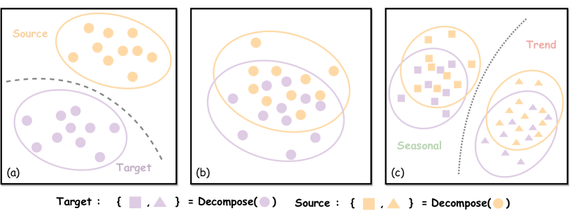
Figure 1: Comparison between previous adaptation models and our decomposition adaptation in the feature space. (a) The entangled features of source and target domain before adaptation. (b) Previous adaptation models align the entangled features directly. (c) Our method performs corresponding adaptation on the decomposed features.

Based on the above motivations, we propose a Sequence Decomposition Adaptation Network. The core idea is that we decompose the entangled features, and then design adaptation methods respectively for the decomposed components. Specifically, inspired by contrastive learning (He et al., 2020b), we design Implicit Contrastive Decomposition (ICD), which decomposes the encoded features into seasonal features component and trend features component for further adaptation. During the decomposition process, the transferable part and non-transferable part of the conditional distribution are also separated. The seasonal features contain marginal distribution and transferable conditional distribution. For seasonal features, we perform joint probability adaptation. In the meanwhile, the trend features contain marginal distribution and non-transferable conditional distribution. Therefore, we design Optimal Local Adaptation (OLA) for the trend feature, which formalizes the adaptation problem as a global optimal matching problem, so as to realize that only the temporal-invariant distribution (marginal distribution) will be transferred during adaptation. The decomposition adaptation in the feature space is shown in Figure 1. The SeDAN follows the encoder-decoder structure and utilizes the vanilla Transformer as the base model. The main contributions of this work are as follows:

1. For cross-domain transfer in time series forecasting, we propose a SeDAN model to learn general knowledge including marginal distribution and the transferable part of conditional distribution of features. We adapt the decomposed features respectively with joint probability adaptation and a novel Optimal Local Adaptation to avoid learning non-transferable knowledge.

2. To decompose features for further adaptation, we design feature-level Implicit Contrastive Decomposition, utilizing the idea of contrastive learning to generate seasonal features component and trend features component.

3. We conduct extensive experiments to demonstrate the performance of the SeDAN on five multivariate time series forecasting datasets. The experimental results verify the effectiveness and stability of the SeDAN. We also use visualization methods to show the significance of decomposition adaptation in feature space.

2 Related Work

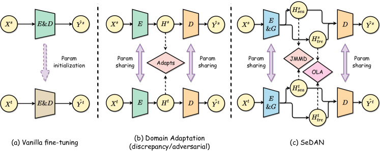
Figure 2: Comparison on structures between the existing transfer learning models and our proposed SeDAN. (a) Vanilla fine-tuning: trains a model on target domain but initialising it with pre-trained weights obtained from training it on the source domain. (b) Domain Adaptation: designs the discrepancy-based or adversarial-based adaptation models to reduce the distance of distributions across domains at the feature-level. (c) Our SeDAN: performs the corresponding adpation methods (JMMD for seasonal features and OLA for trend features) to adapt the decomposed features across domains.

Time Series Forecasting

Nseural forecasting models begin to show advantages in handling data with complex patterns. There are three main types of existing neural forecasting models, which are RNN-based models (Hochreiter and Schmidhuber, 1997; Chung et al., 2014; Lai et al., 2018), TCN-based models (van den Oord et al., 2016; Bai et al., 2018, 2019) and Transformer-based models (Zhou et al., 2021; Lim et al., 2019; Wu et al., 2020; Li et al., 2019). The RNN-based models often utilize gated units to alleviate the long-term dependency (Zhou et al., 2021) and follow the Seq2Seq models (Li et al., 2019; Guen and Thome, 2020) for multi-horizon forcasting. Another way to relieve the long-term dependency is to employ skip connections (Chang et al., 2017) or multi-scale dependency (Chen et al., 2021). However, the sequential dependency issue of the RNN-based models makes it hard to parallelize. Through the causal convolution, TCN maintains parallelism in processing time series data, but the model scalability in handling long-term dependency still remains limited. Through self-attention mechanism, the Transformer-based models (Vaswani et al., 2017) reduce the traveling path between the current signal and the historical signal to $O(1)$. However, the high computational complexity becomes the bottleneck. To reduce the computational cost, prior works (Torralba and Efros, 2011; Kitaev et al., 2020) design the unstructured sparse attention by introducing local correlation assumptions. Zhou et al. propose Informer with a structured sparse attention from the perspective of activity differences for the distribution.

Transfer Learning and Domain adaptation

Transfer learning relaxes the I.I.D. assumption between training data and test data, aiming to learn general knowledge from the source domains which are similar to the target domain. The knowledge transfer in time series forecasting is related to the Domain Adaptation (DA) (Tzeng et al., 2014), which assumes that the marginal distribution of data between source and target domain is different. There are three types of methods to deal with DA (Zhao et al., 2022), including Discrepancy-based, Adversarial-based and Generative-based methods. The Discrepancy-based and Adversarial-based methods both focus on reducing the distance of feature-level distributions between two domains. The difference is that the Discrepancy-based methods use a explicit metric function to define the distance between two domains. In contrast, the Adversarial-based methods use the adversarial training to replace the metric function with a neuralized discriminator.

Recently there has been some works focusing on knowledge transfer in time series (Jin et al., 2021; Ye and Dai, 2021; Wilson et al., 2021; Ragab et al., 2021; Liu and Xue, 2021; Cai et al., 2021). Liu and Xue propose a hybrid spectral kernel network based on spectral theorem and kernel approximation to perform alignment across domains. Wilson et al. utilize adversarial training to align the feature-level distribution across domains, and design a contrastive learning algorithm to leverage cross-source label information. However, these models only focus on time series classification. For the time series forecasting, Ye and Dai utilize the Dynamic Time Warping and Jensen-Shannon to measure the similarity between datasets and embed the transferring stage into the feature learning process. Further, Jin et al. take advantage of attention modules and adversarial training to learn the domain-independent features. These methods address partial problems of applying transfer learning to time series forecasting, but do not consider that the stochastic transition dynamics of latent state is hard to transfer. We design a model to decompose the hard-to-transfer conditional distribution, followed by further distribution adaptation. The comparison between our proposed decomposition adaptation model and the existing transfer learning models is shown in Figure 2.

Decomposition

Time series data can be decomposed into a series of components (Cleveland et al., 1990; Huang et al., 1998; Shiskin, 1967; Godfrey and Gashler, 2018). Due to the reduced coupling, feature patterns are more easier to extract. Learning from different components respectively can improve the prediction performance of the model. Cleveland et al. design a Seasonal and Trend Decomposition Procedure based on Loess (STL), using robust locally-weighted regression as a smoothing method. Huang et al. propose an Empirical Mode Decomposition mothod that is not based on basis functions but only relies on local characteristic time scale. The above methods all design an explicit structure to decompose sequences. Godfrey and Gashler present a neural decomposition model, which uses neural networks to conduct the decomposition of periodic and aperiodic terms. Different from our work, this model only handles univariate sequence in the time domain. We propose ICD that can handle more complex multivariate sequence in feature level.

Contrastive Learning

Contrastive learning is a type of self-supervised learning (Liu et al., 2020), which learns similarity between samples with the same attribute. Related works have been used for many tasks of time series (Wilson et al., 2021; Eldele et al., 2021; Tonekaboni et al., 2021; Franceschi et al., 2019). Tonekaboni et al. propose a Temporal Neighborhood Coding that exploits local smoothness during temporal signal generation to learn generalizable representations of windows. Eldele et al. design a context-based contrast module, which maximizes the similarity between different contexts in the same sample while minimizing the similarity between the contexts in different samples to learn robust temporal representations. In this paper, our proposed model utilizes contrastive learning to decompose features instead of learning the general feature representations.

3 Preliminary

This paper focuses on the Transfer Learning in time series forecasting. Before introducing our method, we provide the problem definition. Single-source transfer learning is discussed in this paper. Given a set of time series data as the target domain data $D^{t}=\{X^{t},Y^{t}\}$, we have $X^{t}=(x_{1}^{t},x_{2}^{t},\cdots,x^{t}_{l_{tx}})\in\mathbb{R}^{l_{tx}\times d_{tx}}$ and $Y^{t}=(y_{1}^{t},y_{2}^{t},\cdots,y^{t}_{l_{ty}})\in\mathbb{R}^{l_{ty}\times d_{ty}}$, where $d_{tx}\geqslant 1$ and $d_{ty}\geqslant 1$ represent the dimension of time series data. In addition , we have a set of source domain data $D^{s}=\{X^{s},Y^{s}\}$, where $X^{s}\in\mathbb{R}^{l_{sx}\times d_{sx}}$ and $Y^{s}\in\mathbb{R}^{l_{sy}\times d_{sy}}$. The dimensions $d_{tx}$ and $d_{sx}$, $d_{ty}$ and $d_{sy}$ are not necessarily equal. Both of $D^{s}$ and $D^{t}$ are time series data, and we assume that they share the same feature space, which can be expressed as $\mathcal{X}^{s}=\mathcal{X}^{t}$, but have different marginal distributions $P_{s}\left(X^{s}\right)\neq P_{t}\left(X^{t}\right)$ because of the Covariate Shift [57]. Besides, due to the different stochastic transition dynamics of latent state, we consider that the conditional distributions are also different: $P_{s}\left(Y^{s}|X^{s}\right)\neq P_{t}\left(Y^{t}|X^{t}\right)$ , which leading to the Dataset Shift [58] in the task. Our goal is to exploit both $D_{t}$ and $D_{s}$ to learn forecasting model for the target domain, mitigating the impact of Dataset Shift.

4 Methodology

In this section, we propose a Sequence Decomposition Adaptation Network. We introduce the overall structure of SeDAN in subsection 4.1, then, we describe the key modules: the Seasonal-Trend Decomposition module for feature sequences (in subsection 4.2), and the Decomposition Adaption module for the decomposition components (in subsection 4.3).

4.1 Overall Framework

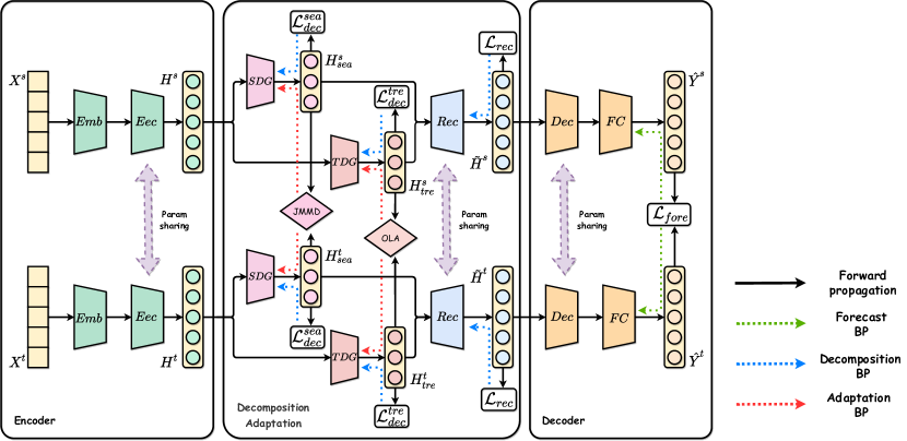
Figure 3: Overall framework of our SeDAN model. We design a Decomposition Adaptation method for knowledge transfer in time series forecasting, containing three parts: the basic Attention-based prediction module (including encoder and decoder), the Decomposition module and the Adaptation module. The dashed arrows describe the training process of the network.

As shown in Figure 3, the SeDAN model consists of three main components, including the basic Transformer-based prediction module, the Seasonal-Trend Decomposition module and the Decomposition Adaptation module. The core idea of SeDAN is that in the knowledge transfer process, we do not directly align the features obtained from the encoder, but align the feature components decomposed from the original encoder features. Due to the low coupling between the feature components, we can apply corresponding adaptation methods to the components respectively. Specifically, for the source domain data $X^{s}$ and the target domain data $X^{t}$, the basic prediction module performs feature encoding to obtain original feature sequences $H^{s}$ and $H^{t}$. Then we design ICD to conduct the Season-Trend Decomposition for original feature sequences. For $H^{s}$, we decompose it into the seasonal feature component $H_{sea}^{s}$ and trend feature component $H_{tre}^{s}$. Similarly, for $H^{t}$, we also decompose it into $H_{sea}^{t}$ and $H_{tre}^{t}$. For the source and target domains, we perform adaptation of the two types of features respectively. We use joint probability adaptation to define the seasonal feature metric $\mathscr{D}^{s}$, by minimizing the distance $<\phi^{u}(H_{sea}^{s}),\phi^{u}(H_{sea}^{t})>^{\mathscr{D}^{s}}$ in the general feature space $\phi^{u}$. And we propose an Optimal Local Adaptation as the trend feature metric $\mathscr{D}^{t}$ , to minimize the distance $<\phi^{u}(H_{tre}^{s}),\phi^{u}(H_{tre}^{t})>^{\mathscr{D}^{t}}$. The knowledge transfer process of SeDAN is mainly reflected in the Seasonal-Trend Decomposition module and the Decomposition Adaptation module. After the knowledge transfer process, we reconstruct the original encoder features using the seasonal and trend features, and use the reconstructed $\tilde{H}^{s}$ and $\tilde{H}^{t}$ for prediction.

The basic prediction model of SeDAN is built on the encoder-decoder framework. The encoder generates the corresponding feature sequence $H=(h_{1},h_{2},\cdots,h_{t})$ for the input time series $X$ , while the reconstructed $H$ is the input of the decoder to generate prediction results $\hat{Y}$. In this paper, we use vanilla Transformer to construct our model. We utilize stacked self-attention structure [14] and position-wise feed forward network as encoder, and utilize masked self-attention as decoder. We use Local Time Stamp and Global Time Stamp (Zhou et al., 2021) as Positional Encoding.

In the learning process of SeDAN, the objective function consists of three parts. We define MSE as the objective function of basic prediction learning, define infoNCE Loss for decomposition learning, and define $\mathscr{D}^{s}$ and $\mathscr{D}^{t}$ for feature adaptation. Based on the above items, the final objective function of SeDAN can be formalized as follows:

$$\mathcal{L}=\underbrace{\mathcal{L}_{mse}\left(\hat{\mathbf{Y}},\mathbf{Y}\right)}_{\text{forecasting }}\\ +\lambda\underbrace{\mathcal{L}_{dec}\left(\mathbf{H}^{s},\mathbf{H}^{t}\right)}_{\text{decomposition }}\\ +\gamma\underbrace{\mathcal{L}_{\mathscr{D}^{s},\mathscr{D}^{t}}\left(\mathbf{H}_{sea},\mathbf{H}_{tre}\right)}_{\text{adaptation }},$$ (1)

where $\lambda$ represents the decomposition ratio and $\gamma$ represents the adaption ratio, both of which are hyper parameters.

During inference, we only keep the neural networks for the target domain data.

4.2 Implicit Contrastive Decomposition

In this subsection, we introduce the proposed ICD for the Seasonal-Trend Decomposition. In this module, the feature sequence extracted by encoder is decomposed into low-coupling seasonal and trend features for follow-up decomposition adaptation. The original feature sequence $H$ contains the entangled seasonal feature $H_{sea}$ and the trend feature $H_{tre}$. In order to obtain $H_{sea}$ and $H_{tre}$, we design Seasonal Decomposition Generator (SDG) and Trend Decomposition Generator (TDG). It is necessary to find an efficient way to make the generated features have periodic properties and trend properties respectively. Besides, the model should be able to reconstruct the original feature sequence with the two generated features in order to prevent information loss.

Since the seasonal and trend features are difficult to define explicitly, inspired by contrastive learning (Liu et al., 2020; He et al., 2020c; Chen et al., 2020), we design an Instance-Instance Contrast method called ICD. The method captures the periodic property invariance and trend property invariance between instances to construct the self-supervised objective functions for SDG and TDG. Specifically, we construct a dictionary look-up task. For the $H$ as input, the positive samples $K_{i}^{+}$ are generated by data augmentation that maintains the periodicity and trend of the input sequence. And the negative samples $K_{i}$ are sampled from other sequences in the mini-batch. We put $H$ pass through the data augmentation and the generators to construct the query of the look-up task, and regard the $K_{i}^{+}$ and $K_{i}$ as keys, so as to construct a contrastive learning task for SDG and TDG. In order to improve the effectiveness of contrastive learning, we construct a memory bank with negative samples by a queue. In order to ensure the consistency of negative samples in the memory bank, we refer to MoCo [52] and use a momentum encoder to generate keys. Different from MoCo, when a new batch of data needs to enter the queue, we no longer use a simple first-in-first-out method, but use an Online Prototype Update (OPU) mechanism. The time series dataset is relatively small, and directly discarding the first-in samples leads to a decrease in the richness of negative samples. Therefore, we aim to use the samples effectively through OPU. For $K_{i}$ which will be discarded from the queue, OPU selects the most similar sample $K_{j}$ from the existing keys of memory bank as the prototype, and then fuse $K_{i}$ and $K_{j}$ to update the prototype, leading to a more representative prototype. The calculation of OPU can be formulized as follows:

$$\mathop{\arg\min}_{K_{j}} =\frac{<K_{i},K_{j}>^{\mathscr{D}^{opu}}}{\sum_{j=1}^{N_{b}}<K_{i},K_{j}>^{\mathscr{D}^{opu}}},$$ (2)

$$K_{j} =(1-\beta)K_{j}+\beta K_{i},$$

where $N_{b}$ is the capacity of the memory bank and $\beta$ is the update ratio. We use the dot product as $\mathscr{D}^{opu}$.

Then we introduce the decomposition generators of seasonal and trend features in detail.

Seasonal feature decomposition

We define MLP as the SDG to generate the seasonal feature $H_{sea}$:

$$H_{sea}=MLP^{SDG}(H).$$ (3)

We leverage the above method to provide supervision for SDG. In the process of constructing positive samples, we choose data augmentation methods that can maintain the periodicity of input sequence, including rolling, flipping, and scaling (Wen et al., 2021). For the input feature sequence $H$, the relevant methods are specifically defined as follows:

• Rolling: scroll the sequence on the time axis. If we move the sequence $h$ for $r$ time steps, the items in new sequence are $h_{i}=h_{i-Sgn(i-r)\cdot r}$.

• Flipping: flip the sequence horizontally, and the items in new sequence are $h_{i}=h_{m-i-1}$.

• Scaling: scale the sequence elements, and the items in new sequence are $h_{i}=\epsilon_{s}\cdot h_{i}$.

The above data augmentation methods do not alter the inherent periodicity of the sequence. We use a combination of these methods to generate the query and positive samples of seasonal feature:

$$Q^{sea} =MLP^{SDG}(f^{sea}_{da}(H)),$$ (4)

$$K^{sea+} =MLP^{Moco}(f^{sea}_{da}(H_{i})),$$

where $f^{sea}_{da}$ represents the combined data augmentation process for seasonal decomposition. $MLP^{Moco}$ and $MLP^{SDG}$ have the same structure but momentum update is used for $MLP^{Moco}$ . At the same time, we sample $k$ negative samples from the memory bank. For positive samples $K^{sea+}$ and the negative samples $\{K_{1}^{sea},K_{2}^{sea},\cdots,K_{k}^{sea}\}$, we use infoNCE Loss as the contrastive loss function:

$$\mathcal{L}_{dec}^{sea}=-\log\frac{\exp\left(Q^{sea}\cdot K^{sea+}/\tau\right)}{\exp\left(Q^{sea}\cdot K^{sea+}/\tau\right)+\sum_{j=1}^{k}\exp\left(Q^{sea}\cdot K_{j}^{sea}/\tau\right)},$$ (5)

where $\tau$ is the temperature hyper parameter. To enrich the diversity of keys, we randomly combine the above three data augmentation methods to generate positive samples.

Trend feature decomposition

For the TDG, inspired by the STL (Cleveland et al., 1990), we use the causal convolution (Bai et al., 2018) and average pooling to simulate the trend smoothing process. The generation process of the trend feature $H_{tre}$ is formulized as:

$$H_{tar}=AvgPool(Conv_{causal}^{TDG}(H)).$$ (6)

Similar to SDG, we also construct a contrastive method to provide supervision for TDG. We choose the data augmentation methods that maintain the trend of the sample sequence to construct positive samples, including jittering, window cropping, and window warping (Wen et al., 2021). The specific definitions are as follows:

• Jittering: add random noise to the sequence, and the the items in new sequence are $h_{i}=h_{i}+\epsilon_{j}^{i}$, where $\epsilon_{j}^{i}\sim\mathcal{N}(0,\sigma^{2}_{j})$.

• Window cropping: randomly extract consecutive slices from the original sequence as the augmented sequence.

• Window warping: choose a random time range of the original sequence and then compress or expand while keeping the other time ranges unchanged.

For positive samples $K^{tre+}$ and negative samples $\{K_{1}^{tre},K_{2}^{tre},\cdots,K_{k}^{tre}\}$, we also use infoNCE as a contrastive loss function $\mathcal{L}^{tre}_{dec}$, which formula has a similar form to $\mathcal{L}_{dec}^{sea}$ .

After generating the decomposed components $H_{sea}$ and $H_{tre}$, we reconstruct the components as $\tilde{H}$ using the reconstructor and KL divergence. We hope $\tilde{H}$ to keep the information contained in the original feature sequence $H$ as much as possible. Therefore, we can obtain the complete objective function of the ICD as:

$$\mathcal{L}_{dec}=\mathcal{L}_{dec}^{sea}+\mathcal{L}_{dec}^{tre}+\mathcal{L}_{KL}(H||\tilde{H}).$$ (7)

It should be noted that since we use implicit decomposition generation instead of explicit decomposition (Cleveland et al., 1990; Huang et al., 1998; Shiskin, 1967), the decomposed seasonal and trend features no longer satisfy the additive or multiplicative model. The reconstruction helps SeDAN to reduce information loss during decomposition.

4.3 Decomposition Adaptation

The Decomposition Adaptation is carried out under the assumption that the marginal distributions of different time series are transferable and the conditional distributions are partly transferable. Because the seasonal features reflect the periodicity of the sequence, the stochastic transition dynamics is relatively fixed, which can be transferred. In contrast, the transition dynamics in the trend features is more related to the domain characteristic, and directly transferring the trend features may lead to negative transfer. Based on the above reasons, we argue that the seasonal features include the marginal distribution and the transferable conditional distribution of the sequence, while the trend features include the marginal distribution and the non-transferable conditional distribution. Under this assumption, we design different adaptation methods for seasonal and trend features separately, which aim to only adapt the transferable part in different domains. We introduce the adaptation methods for the two types of features respectively in subsection 4.3.1 and 4.3.2.

4.3.1 Seasonal Feature Adaptation

The Seasonal Feature Adaptation is to align the seasonal features $H_{sea}^{s}$ in source domain and $H_{sea}^{t}$ in target domain. We argue that subsequences can better reflect the characteristic patterns in sequence data than a single time step. Through observation, it can be found that subsequences in the same or different time series often have similar morphology in the time domain. The powerful performance of the forecasting algorithms based on the sliding window also shows the rationality of this assumption. More recently, Du et al. formalize this distribution assumption, defining it as the Temporal Covariate Shift. In our work, we use the subsequence-based distribution assumption.

For the seasonal feature sequence, such as $H_{sea}^{t}$ in the target domain, we split it into $n_{t}$ subsequences: $H_{sea}^{t}=\{Se^{t}_{1},Se^{t}_{2},\cdots,Se^{t}_{n_{t}}\}$. We consider that each subsequence $Se_{i}^{t}$ reflects the marginal distribution in the sequence, and the conversion method between consecutive subsequences reflects the conditional distribution. Similarly for the source domain, we also have $H_{sea}^{s}=\{Se^{s}_{1},Se^{s}_{2},\cdots,Se^{s}_{n_{s}}\}$ with $n_{s}$ subsequences. Since the distribution contained in seasonal features is fully transferable, we can adapt the two distributions at the same time. Therefore, we define the joint distribution adaptation as the adaptation method of $H_{sea}^{s}$ and $H_{sea}^{t}$. Considering the properties of time series data, we use the first-order markov property to simplify the Joint Maximum Mean Discrepancy (JMMD) [62] as the seasonal metric $\mathscr{D}^{s}$. The adaptation metric of $H_{sea}^{s}$ and $H_{sea}^{t}$ in the feature space can be calculated as follows:

$$\mathscr{D}^{s}(H_{sea}^{s},H_{sea}^{t}) =\frac{1}{n_{s}}\sum_{i=1}^{n_{s}}k_{e}\left(Se_{i}^{s},Se_{j}^{s}\right)$$ (8)

$$+\frac{1}{n_{t}}\sum_{i=1}^{n_{t}}k_{e}\left(Se_{i}^{t},Se_{j}^{t}\right)$$

$$+\frac{2}{n_{s}n_{t}}\sum_{i=1}^{n_{s}}\sum_{j=1}^{n_{t}}k_{e}\left(Se_{i}^{s},Se_{j}^{t}\right),$$

where $k_{e}$ is the kernel function used to regenerate the inner product transformation in the kernel hilbert space, and we use gaussian kernel in this paper. The first-order markov property effectively reduces the computational complexity of JMMD.

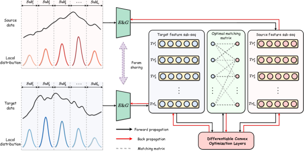
Figure 4: The proposed OLA adaptation module. Following the subsequence-based distribution assumption, the trend feature adaptation is achieved by matching subsequences with similar distributions in the source and target domains.

4.3.2 Trend Feature Adaptation

The Trend Feature Adaptation is to align $H_{tre}^{s}$ and $H_{tre}^{t}$. Different from the Seasonal Feature Adaption, the conditional distributions contained in $H_{tre}^{s}$ and $H_{tre}^{t}$ are more difficult to transfer. Only the marginal distributions can be transferred to help the model learn domain-independent knowledge. Because the subsequences with similar features may have different indices in the two sequences, it is unreasonable to adapt the marginal distribution directly to the sequential $H_{tre}^{s}$ and $H_{tre}^{t}$, which can be formulized as $\sum_{i=1}^{t}\mathscr{D}^{t}(h_{i}^{s},h_{i}^{t})$. If the order measurement based on the global representation is directly performed, the model will discard the local features in the sequence when learning domain-independent feature representations, which are critical for time series forecasting. Therefore, we propose OLA to deal with the problem that similar subsequences have different indices so as to retain meaningful local characteristics during the transfer process.

The OLA also follows the subsequence-based distribution assumption, and each subsequence is regarded as a local characteristic in the complete sequence. OLA formulates the adaptation problem as a global optimal matching problem and solves it using a linear programming method. In the global scope, similar matching subsequences are found for two sets of feature subsequences in the source domain and the target domain to achieve trend feature adaptation. Specifically, for $H_{tre}^{s}=\{Tr^{s}_{1},Tr^{s}_{2},\cdots,Tr^{s}_{n_{s}}\}$ and $H_{tre}^{t}=\{Tr^{t}_{1},Tr^{t}_{2},\cdots,Tr^{t}_{n_{t}}\}$, we define the cost matrix $C\in\mathbb{R}^{n_{s}\times n_{t}}$, where $c_{i}^{j}$ represents the matching cost between subsequences $Tr^{s}_{i}$ and $Tr^{t}_{i}$. We hope to find a matching matrix $M\in\mathbb{R}^{n_{s}\times n_{t}}$, so that the matched two sets of subsequences have the minimum matching cost under constraints. Because we aim to find the similar match between two sets of subsequences, we can define the cost matrix $C=A-S$, where $A=\{a_{ij}=1|i=1,2,\cdots n_{s},j=1,2,\cdots n_{t}\}$, and $S\in\mathbb{R}^{n_{s}\times n_{t}}$ is the similarity matrix between the two sets of subsequences. We formalize the optimal matching problem and the constraints as follows:

$$\underset{m_{ij}}{\operatorname{minimize}} \sum_{i=1}^{n_{s}}\sum_{j=1}^{n_{t}}(1-s_{ij})m_{ij},$$ (9)

s.t. $$m_{ij}\geq 0,\quad i=1,\cdots,n_{s},j=1,\cdots,n_{t},$$

$$\sum_{i=1}^{n_{s}}m_{ij}=1,\quad j=1,\ldots n_{t},$$

$$\sum_{j=1}^{n_{t}}m_{ij}=1,\quad i=1,\ldots n_{s}.$$

Cosine similarity is used to define the similarity matrix $S$:

$$s_{ij}=\frac{Tr^{s}_{i}\odot Tr^{t}_{j}}{\|Tr^{s}_{i}\|\times\left\|Tr^{t}_{i}\right\|},$$ (10)

where $\odot$ represents element-wise multiplicatio between matrices. The optimal matching problem is a standard Linear Programming problem whose Lagrangian can be expressed as:

$$L(M,\nu,\lambda)=(A-S)^{T}M+\nu^{T}(AM-b)+\eta^{T}(GM-h),$$ (11)

where $A$ and $b$ represent the equality constraints in optimization problems. $G$ and $h$ represent the inequality constraints. $\nu$ and $\eta$ are dual variables for equality and inequality constraints. We choose to use the primal-dual interior point method to solve this convex optimization problem. The OLA is used as the trend metric $\mathscr{D}^{t}$. Having the optimal matching matrix $\tilde{M}$, the adaption for $H_{tre}^{s}$ and $H_{tre}^{t}$ is calculated as follows:

$$\mathscr{D}^{t}(H_{tre}^{s},H_{tre}^{t})=(A-S)\odot\tilde{M}.$$ (12)

The optimization problem should be embed into the network to optimize the parameters $\theta$ for learning. Therefore, the Differentiable Convex Optimization Layers is introduced to perform differentiable processing on this optimization problem, so that the gradient can be back-propagated on the optimization layer. The overall OLA adaptation module is shown in Figure 4. We combine $\mathscr{D}^{s}$ and $\mathscr{D}^{t}$ to construct the complete objective function of the adaptation:

$$\mathcal{L}_{\mathscr{D}^{s},\mathscr{D}^{t}}\left(\mathbf{H}_{sea},\mathbf{H}_{tre}\right)=\mathscr{D}^{s}(H_{sea}^{s},H_{sea}^{t})+\mathscr{D}^{t}(H_{tre}^{s},H_{tre}^{t}).$$ (13)

Through decomposition and adaptation, we complete the alignment of source and target domain data in the feature space.

5 Experiments

We validate the performance of our SeDAN on multiple multivariate time series forecasting datasets. In subsection 5.1, we introduce the datasets and the implementation details of the experiments. In subsection 5.2, we introduce the comparison methods including the single-domain baselines and the cross-domain baselines. In subsection 5.3, we report the results and provide detailed analysis of the experiments. In subsection 5.4 and 5.5, we conduct ablation experiments and further analyze the properties of our proposed model.

Table 1: Performance comparison with single-domain methods on five target datasets.

Models		SeDAN(Best)		SeDAN(Avg)		Informer		TCN		LSTNet		LSTMa
Metric		MSE	MAE	MSE	MAE	MSE	MAE	MSE	MAE	MSE	MAE	MSE	MAE
ETTh1	24	0.491	0.499	0.509	0.509	0.577	0.549	0.583	0.547	1.293	0.901	0.650	0.624
	48	0.592	0.555	0.611	0.567	0.685	0.625	0.670	0.606	1.456	0.960	0.702	0.675
	168	0.827	0.688	0.834	0.693	0.931	0.752	0.811	0.680	1.997	1.214	1.212	0.867
ETTh2	24	0.389	0.480	0.425	0.502	0.720	0.665	0.935	0.754	2.742	1.457	1.143	0.813
	48	0.746	0.700	0.788	0.715	1.457	1.001	1.300	0.911	3.567	1.687	1.671	1.221
	168	1.691	1.013	1.737	1.037	3.489	1.515	4.017	1.579	3.242	2.513	4.117	1.674
WTH	24	0.316	0.340	0.312	0.354	0.335	0.381	0.321	0.367	0.615	0.545	0.546	0.570
	48	0.369	0.409	0.373	0.414	0.395	0.459	0.386	0.423	0.660	0.589	0.829	0.677
	168	0.503	0.502	0.503	0.504	0.608	0.567	0.491	0.501	0.748	0.647	1.038	0.835
EXC	24	0.166	0.315	0.187	0.343	0.338	0.460	0.499	0.452	0.576	0.581	0.504	0.440
	48	0.455	0.541	0.541	0.600	0.847	0.752	1.759	1.130	1.551	1.058	1.473	0.946
	168	0.726	0.688	0.735	0.695	0.972	0.766	2.462	1.659	1.822	1.212	1.776	1.181
ILI	24	3.196	1.230	3.335	1.268	5.764	1.677	6.624	1.830	6.026	1.770	5.924	1.710
	36	3.069	1.186	3.284	1.223	4.755	1.467	6.858	1.879	5.340	1.668	6.416	1.794
	60	3.710	1.298	3.807	1.333	5.264	1.564	7.127	1.918	5.548	1.720	6.736	1.833

5.1 Datasets and implementations

5.1.1 Datasets

We extensively evaluate the proposed SeDAN on 5 real-world benchmark datasets.

• ETT (Electricity Transformer Temperature) (Zhou et al., 2021): The ETT dataset collects electricity transformer data from two different counties in China between July 2016 and July 2018, including the oil temperature and six other electricity load features. ETT consists of two 1-hour-level datasets {ETTh1, ETTh2} and two 15-minute-level datasets {ETTm1, ETTm2}. Only ETTh1 and ETTh2 are used in our experiments.

• Weather: The Weather dataset collects local climate data from nearly 1,600 U.S. locations between 2010 and 2013, including the wet bulb and the remaining 11 climate features. The data points are collected hourly.

• Exchange-Rate(Lai et al., 2018): The Exchange-Rate dataset collects daily exchange rates for eight different countries from 1990 to 2016.

• ILI (Influenza-like Illness)(Wu et al., 2021): The ILI dataset collects weekly data on influenza-like illness (ILI) patients in the United States from 2002 to 2021, including seven features such as the proportion and total number of ILI patients.

To verify the effectiveness of the proposed model, we set up single-domain and cross-domain comparative experiments respectively. In the single-domain experiment, the compared models only use the target domain dataset for training and inference. In the cross-domain experiment, we choose the above datasets as the target datasets and set at least three source datasets for each target dataset separately, which follows the rule that the size of the source dataset is roughly equal or larger than the size of the target dataset. Due to the large scale of data in the WTH dataset, we choose a larger ECL dataset (Zhou et al., 2021) as one of its source datasets, which collects the hourly electricity consumption of 321 customers from 2012 to 2014.

Table 2: Performance comparison with cross-domain methods on five target datasets, each with three source datasets.

Model			SeDAN		DAN		JAN		Fine-tuning		vanilla Trx
Target	Length	Source	MSE	MAE	MSE	MAE	MSE	MAE	MSE	MAE	MSE	MAE
ETTh1	24	ETTh2	0.512	0.510	0.568	0.521	0.572	0.522	0.550	0.525	0.583	0.556
		WTH	0.491	0.499	0.559	0.522	0.531	0.501	0.501	0.499
		ECL	0.522	0.516	0.555	0.535	0.576	0.523	0.564	0.556
	168	ETTh2	0.827	0.688	0.909	0.711	0.894	0.696	0.923	0.729	0.949	0.762
		WTH	0.843	0.698	0.882	0.703	0.901	0.707	0.952	0.750
		ECL	0.830	0.690	0.969	0.753	0.875	0.699	0.929	0.736
ETTh2	24	ETTh1	0.389	0.480	0.517	0.571	0.538	0.568	0.496	0.549	0.747	0.694
		WTH	0.461	0.529	0.467	0.548	0.510	0.550	0.555	0.577
		ECL	0.426	0.497	0.611	0.640	0.588	0.597	0.614	0.606
	168	ETTh1	1.772	1.092	2.853	1.413	2.089	1.168	3.794	1.641	3.569	1.516
		WTH	1.748	1.007	2.275	1.233	1.834	1.042	2.678	1.287
		ECL	1.691	1.013	3.129	1.485	2.176	1.167	3.396	1.528
WTH	24	ETTh1	0.316	0.340	0.320	0.370	0.334	0.360	0.340	0.397	0.348	0.398
		ETTh2	0.312	0.364	0.338	0.387	0.340	0.369	0.332	0.383
		ECL	0.308	0.359	0.322	0.373	0.346	0.367	0.330	0.383
	168	ETTh1	0.506	0.504	0.543	0.541	0.555	0.546	0.559	0.562	0.617	0.572
		ETTh2	0.503	0.502	0.539	0.539	0.557	0.549	0.532	0.530
		ECL	0.499	0.507	0.580	0.577	0.561	0.556	0.549	0.549
EXC	24	ETTh1	0.166	0.315	0.355	0.454	0.248	0.408	0.211	0.369	0.341	0.464
		ETTh2	0.207	0.365	0.322	0.426	0.283	0.431	0.261	0.397
		WTH	0.188	0.350	0.265	0.399	0.213	0.374	0.211	0.361
	168	ETTh1	0.728	0.694	0.996	0.738	0.775	0.707	0.757	0.716	0.981	0.781
		ETTh2	0.726	0.688	0.806	0.703	0.770	0.710	0.971	0.742
		WTH	0.750	0.702	0.888	0.711	0.887	0.745	1.100	0.770
ILI	24	ETTh1	3.196	1.230	4.649	1.435	3.597	1.214	5.351	1.542	5.821	1.687
		WTH	3.480	1.287	3.621	1.277	4.198	1.427	5.743	1.630
		ECL	3.330	1.286	4.172	1.399	3.675	1.245	5.377	1.580
	60	ETTh1	3.710	1.298	4.193	1.413	4.727	1.433	4.825	1.415	5.311	1.581
		WTH	3.799	1.345	4.920	1.481	4.221	1.338	5.003	1.438
		ECL	3.913	1.357	3.984	1.411	4.257	1.366	5.296	1.479

5.1.2 Implementation details

Our experiments focus on multivariate time series forecasting task. All datasets are splited into training, validation and test set in chronological order by the ratio of 6:2:2 for ETTh1 and ETTh2 dataset and 7:1:2 for the other datasets. Our SeDAN uses 3-layer encoder and 2-layer decoder on the WTH dataset due to its large scale, and use 2-layer encoder and 1-layer decoder on the rest. The Adam is used for parameter optimization. The initial learning rate is in $\{10^{-4},10^{-5}\}$ and the learning rate decay and early stopping is used for 20 epochs. The hyper parameters $\lambda$ and $\gamma$ are both set to 0.1. We utilize the qhth tool (Amos and Kolter, 2017) to implement the differentiable convex optimization procedure in SeDAN. We use $\mathrm{MSE}=\frac{1}{n}\sum^{n}_{i=1}{(y-\hat{y})^{2}}$ and $\mathrm{MAE}=\frac{1}{n}\sum^{n}_{i=1}{\lvert y-\hat{y}\rvert}$ as the evaluation metrics. Our code is implemented on PyTorch and the experiments are performed on two Nvidia Titans 24GB GPUs.

5.2 Comparison methods

We compare our SeDAN with the following single-domain and cross-domain baselines.

Single-domain baselines

We select 4 single-domain models trained only on the target dataset, including LSTNet (Lai et al., 2018), TCN (Bai et al., 2018), and two attention-based models: LSTMa (Bahdanau et al., 2015) and Informer (Zhou et al., 2021).

Cross-domain baselines

In the cross-domain experiments, we use the vanilla Transformer (Vaswani et al., 2017) model as the basic model, using the Local Time Stamp and Global Time Stamp as the position embeddings. The cross-domain baselines include the following: 1) Fine-tuning: the basic model which trains only on the source domain, and finetunes the encoder and decoder on the target domain; 2) DAN (Long et al., 2015): the basic model which uses MK-MMD for adaptation on encoder features of different domain datasets without decomposition; 3) JAN (Long et al., 2017): consistent with the settings of 2), except using JMMD for cross-domain adaptation instead of MK-MMD.

5.3 Main results

Table 1 shows the comparative experimental results on single-domain setting, while Table 2 shows the results on cross-domain setting. In Table 1, we can find that the proposed SeDAN outperforms all single-domain methods compared, achieving an average reduction of 27.0% (MSE) and 16.5% (MAE). In Table 2, we can find that the transfer-based cross-domain baselines are usually better than the single-domain methods, which proves that the cross-domain alignment of features can help the model learn more knowledge and alleviate the problem of insufficient data. Our proposed SeDAN still achieves the best performance in cross-domain experiments. In each experiment setting, we compare our SeDAN with the best performing cross-domain baselines and obtain an average reduction of 10.9% (MSE) and 5.3% (MAE). From table 2, we observe that the three transfer-based baselines do not always achieve performance improvement compared with vanilla Transformer. There may be performance decrease due to the use of source domain data, which means the negative transfer occurs. Because these cross-domain baselines adapt the marginal and conditional distributions together during the transfer process, ignoring the difficulty of transferring conditional distributions in different datasets. In contrast, our proposed SeDAN benefits from not adapting the conditional distribution within the trend features, so that the model can obtain a relatively stable performance improvement. In the case of using different source datasets, the performance of SeDAN has improved or at least remained the same, which shows its ability to effectively reduce the impact of negative transfer. This is beneficial for cross-domain transfer in time series forecasting.

5.4 Ablation Study

Based on ILI and ETTh2 as target datasets, we perform additional ablation experiments to demonstrate the effectiveness of each module in SeDAN.

Table 3: Ablation study of the Decomposition Adaptation method.

Methods	Dataset	ETTh2(24)			ILI(24)
	Source	ETTh1	WTH	ECL	ETTh1	WTH	ECL
baseline	MSE	0.680			4.716
	MAE	0.658			1.511
All-JMMD	MSE	0.548	0.592	0.476	3.753	3.970	3.577
	MAE	0.572	0.580	0.541	1.352	1.333	1.313
All-OLA	MSE	0.412	0.481	0.443	3.593	3.426	3.433
	MAE	0.485	0.544	0.497	1.231	1.301	1.278
Contra2Ours	MSE	0.582	0.662	0.889	4.049	3.971	3.691
	MAE	0.609	0.644	0.746	1.355	1.347	1.237
Ours	MSE	0.389	0.461	0.426	3.196	3.480	3.330
	MAE	0.480	0.529	0.497	1.230	1.287	1.286

Table 4: Ablation study of the Implicit Contrastive Decomposition.

Methods	Dataset	ETTh2(24)			ILI(24)
	Source	ETTh1	WTH	ECL	ETTh1	WTH	ECL
baseline	MSE	0.680			4.716
	MAE	0.658			1.511
DAN	MSE	0.517	0.467	0.611	4.649	3.621	4.172
	MAE	0.571	0.548	0.640	1.435	1.277	1.399
JAN	MSE	0.538	0.510	0.588	3.597	4.198	3.675
	MAE	0.568	0.550	0.597	1.214	1.427	1.245
Conv+Minus	MSE	0.453	0.466	0.525	3.274	3.981	3.452
	MAE	0.530	0.508	0.539	1.308	1.427	1.336
Ours	MSE	0.389	0.461	0.426	3.196	3.480	3.330
	MAE	0.480	0.529	0.497	1.230	1.287	1.286

5.4.1 The performance of Decomposition Adaptation

We first conduct ablation experiments to explore the effects of different adaptation methods to verify our hypotheses about trend and seasonal features. In experiments, we design the following variants: 1) baseline: the vanilla Transformer model with our proposed decomposition and reconstruction, but without cross-domain feature adaptation; 2) All-JMMD: the same structure of SeDAN model except that both seasonal and trend features uses joint distribution adaptation; 3) All-OLA: the same structure of SeDAN model except that both seasonal and trend features uses Optimal Local Adaptation; 4) Contra2Ours: same structure but use OLA for seasonal features, and JMMD for trend features, which is contrary to our SeDAN.

Table 3 shows the results of ablation experiments, demonstrating that SeDAN outperforms its variants in all target datasets. We observe that All-OLA performs better in all variants, second only to SeDAN. For seasonal features, compared to JMMD, OLA only transfer the marginal distribution of the features, and may lose some transferable knowledge, resulting a slight drop on performance. However, for trend features, JMMD significantly degrades the performance compared to OLA, and the transfer effect on different source datasets become unstable. The JMMD takes into account the conditional distribution while the stochastic transition dynamics are different to transfer in different domains, so that using JMMD for trend features adaptation is more likely to lead to the negative transfer.

5.4.2 The performance of the Implicit Contrastive Decomposition.

In this subsection, we verify the effectiveness of the proposed ICD. In addition to the baseline proposed in the previous subsection 5.4.1, we design the following variants: 1) DAN or JAN: the vanilla Transformer model consistent with the description in section 5.2, but we use DAN or JAN for undecomposed encoder features adaptation, respectively; 2) Conv+Minus: use the additive-model-based explicit sequence decomposition method, where the trend feature is directly obtained by convolution as same as SeDAN but without our contrastive learning as supervision, while the seasonal feature is obtained by subtracting the trend term from the original features.

As shown in Table 4, our designed decomposition method outperforms Conv+Minus, proving that the proposed ICD can generate low-coupling features with more transferability. Besides, the both decomposition adaptation methods are better than DAN and JAN, which directly adapt the undecomposed features. It shows that adapting the trend and the seasonal feature separately enables the model to better learn the transferable knowledge across domains.

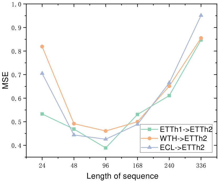
(a) predict-24 task (ETTh2).

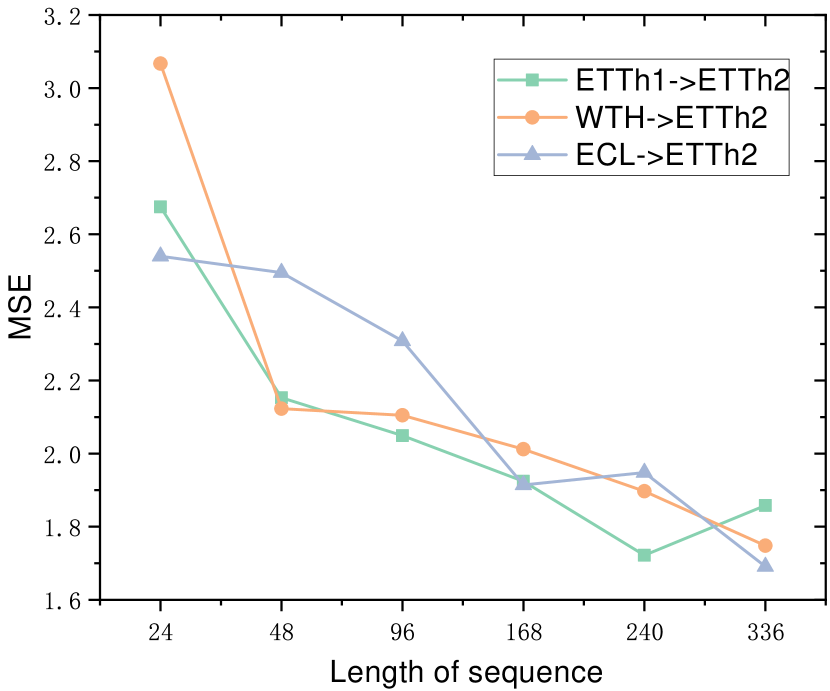
(b) predict-168 task (ETTh2).

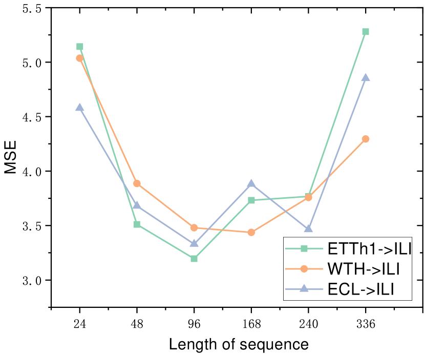
(c) predict-24 task (ILI).

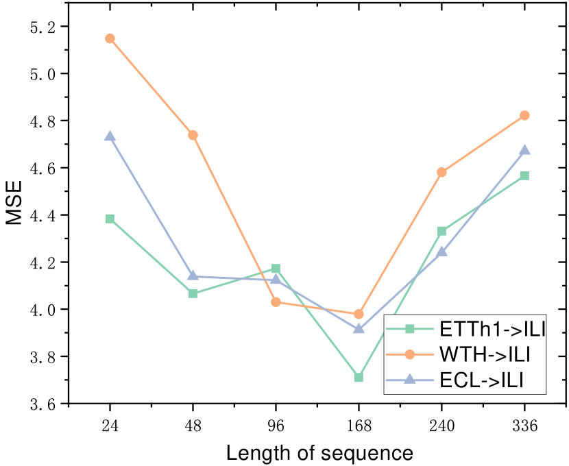
(d) predict-60 task (ILI).

Figure 5: Impact of input sequence length in SeDAN, performance is reported on ETTh2 and ILI.

5.4.3 The impact of Input Sequence Length

Figure 5 shows the impact of different input sequence lengths. At a small prediction length (like 24), with the increasing input length, the forecasting performance on ILI and ETTh2 shows the same trend: MSE first decreased, but with the further increase of input length, MSE begins to rise. Because in the beginning, the richness of the longer input information leads to an increase in the number of learnable local patterns. However, when the input length reaches a certain threshold, it is difficult for self-attention to query effective relevant information from complex local patterns. And the negative impact exceeds the benefit brought by the enrichment of local patterns. When predicting longer sequences, the performance of predict-60 task in ILI keeps the same trend as the predict-24 task, and its optimal input length as 168 in the predict-60 task is longer compared with 96 in the predict-24 task. However, in the predict-168 task of ETTh2, with the increase of input length, the MSE always maintains a downward trend. We consider that the reason is that for ILI, which is a small dataset recorded weekly, providing more old information will increase the difficulty of pattern query, while long-range prediction of ETTh2 requires richer local patterns.

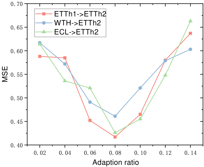
(a) predict-24 task (ETTh2).

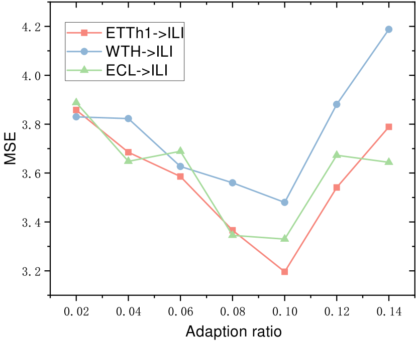
(b) predict-24 task (ILI).

Figure 6: Impact of loss adaption ratio in SeDAN, performance is reported on ETTh2 and ILI.

5.4.4 The impact of loss adaption ratio

Figure 6 shows the forecasting performance of the SeDAN under different adaptation ratios $\gamma$. We observe that on both datasets, as $\gamma$ increases, MSE first decreases and then increases. For ETTh2, the model achieves the best performance at $\gamma=0.08$; and for ILI, the model achieves the best performance at $\gamma=0.10$. Because the ILI dataset is smaller than ETTh2, using a larger $\gamma$ to transfer more knowledge from source domain has a positive impact on the target domain. Besides, the prediction task of ILI is more sensitive to the value of $\gamma$, and the impact of $\gamma$ on the prediction task of ETTh2 is smaller. Compared with ILI, there is a smaller difference between the size of ETTh2 and its source domain datasets, resulting in their different sensitivities to the value of $\gamma$.

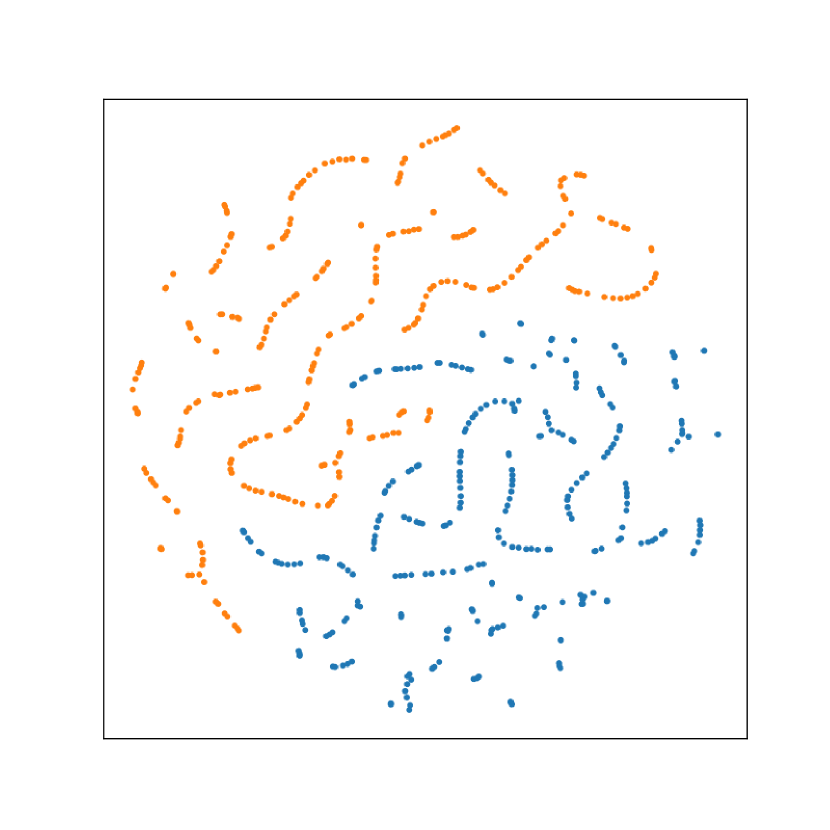
(a) Seasonal features (before).

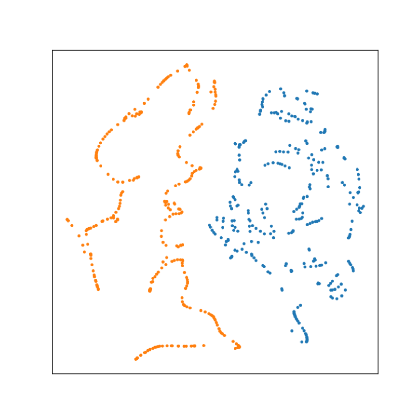
(b) Trend features (before).

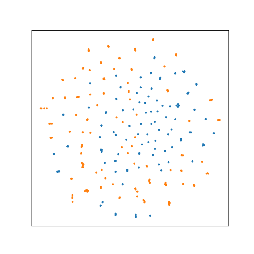
(c) Seasonal features (after).

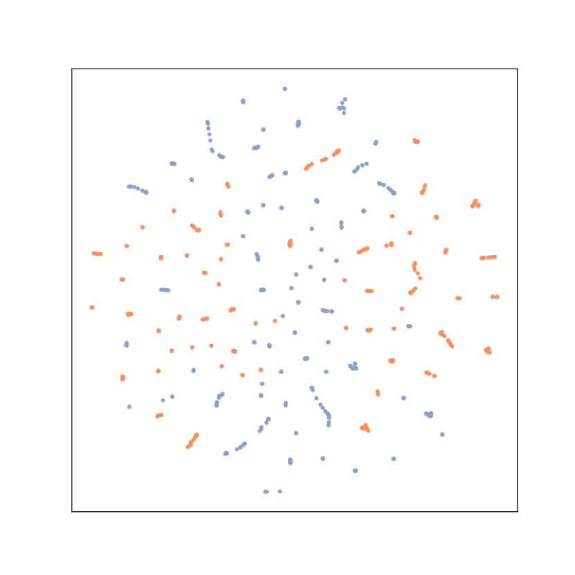
(d) Trend features (after).

Figure 7: Visualization of features distribution before and after decomposition adaptation. ETTh2 (orange points) as target domain and ECL (blue points) as source domain.

5.5 Further Analyses on Our Method

We use the visualization to verify the effectiveness of our SeDAN, use the t-SNE to analyze the influence of proposed Decomposition Adaptation on the feature distribution and further discuss the transferability between datasets.

Adaptation Analysis in Feature Space

We visualize the feature space adaptation on the ETTh2 dataset to illustrate the effectiveness of the Decomposition Adaptation method. Figure 7(a) and Figure 7(b) show the distribution of seasonal and trend features in the source and target domain when only decomposition is performed without adaptation. By comparison, it can be found that the trend features have a certain degree of continuity in the feature space compared with the seasonal features. As shown in Figure 7(c) and Figure 7(d), after feature decomposition in SeDAN, the corresponding features are better adapted by proposed appropriate adaptation methods. Moreover, the distance between the cross-domain features after reconstruction is effectively shortened. The negative transfer problem caused by the non-transferable components in the features is avoided, so that the overall transfer performance is better and more stable.

When to transfer

This paper mainly focuses on what type of knowledge can be transferred across domains in time series forecasting, and how to transfer these knowledge. In this subsection, we briefly analyze the problem of “When to transfer”, which means the performance impact of different sources on the same target domain. As shown in Table 2, when ETTh1 and ETTh2 are chosen as source domains of each other, the performance is better than that using other datasets as source domains because their fields, sampling methods and scales are all similar. Furthermore, the transfer performance tends to be better when the size of the source dataset is larger, possibly due to the increase in the transferable knowledge and local patterns that can be matched. Therefore, we consider that starting from the similarity of the local patterns contained in the dataset is a way to deal with “When to transfer”.

6 Conclusion

In this paper, we explore the transferability of knowledge in cross-domain time series datasets. Starting from the basic problems of transfer learning, we argue the transferable knowledge types between different time series domains, and propose a general transfer framework SeDAN for multivariate time series forecasting. Through the feature-level ICD, we use contrastive learning to decompose the seasonal and trend features. According to their respective transferability, we propose the corresponding decomposition adaptation methods: JMMD for the seasonal features and OLA for the trend features. We conduct experiments on real-world datasets and demonstrate that the proposed SeDAN model can improve the prediction performance on the target domain with the use of different source domains. Compared with general transfer learning methods, SeDAN can provide a more stable transfer effect. This paper mainly focuses on the transferable knowledge types and corresponding transfer methods. In the future, we plan to further explore the problem of “When to transfer” from the perspective of time series similarity.

References

- Amos and Kolter [2017] Brandon Amos and J. Zico Kolter. Optnet: Differentiable optimization as a layer in neural networks. In Doina Precup and Yee Whye Teh, editors, Proceedings of the 34th International Conference on Machine Learning, ICML 2017, Sydney, NSW, Australia, 6-11 August 2017, volume 70 of Proceedings of Machine Learning Research, pages 136–145. PMLR, 2017.
- Bahdanau et al. [2015] Dzmitry Bahdanau, Kyunghyun Cho, and Yoshua Bengio. Neural machine translation by jointly learning to align and translate. In Yoshua Bengio and Yann LeCun, editors, 3rd International Conference on Learning Representations, ICLR 2015, San Diego, CA, USA, May 7-9, 2015, Conference Track Proceedings, 2015.
- Bai et al. [2018] Shaojie Bai, J. Zico Kolter, and Vladlen Koltun. An empirical evaluation of generic convolutional and recurrent networks for sequence modeling. CoRR, abs/1803.01271, 2018.
- Bai et al. [2019] Shaojie Bai, J. Zico Kolter, and Vladlen Koltun. Trellis networks for sequence modeling. In 7th International Conference on Learning Representations, ICLR 2019, New Orleans, LA, USA, May 6-9, 2019. OpenReview.net, 2019.
- Bai et al. [2020] Lei Bai, Lina Yao, Can Li, Xianzhi Wang, and Can Wang. Adaptive graph convolutional recurrent network for traffic forecasting. In Hugo Larochelle, Marc’Aurelio Ranzato, Raia Hadsell, Maria-Florina Balcan, and Hsuan-Tien Lin, editors, Advances in Neural Information Processing Systems 33: Annual Conference on Neural Information Processing Systems 2020, NeurIPS 2020, December 6-12, 2020, virtual, 2020.
- Brown et al. [2020] Tom B. Brown, Benjamin Mann, Nick Ryder, Melanie Subbiah, Jared Kaplan, Prafulla Dhariwal, Arvind Neelakantan, Pranav Shyam, Girish Sastry, Amanda Askell, Sandhini Agarwal, Ariel Herbert-Voss, Gretchen Krueger, Tom Henighan, Rewon Child, Aditya Ramesh, Daniel M. Ziegler, Jeffrey Wu, Clemens Winter, Christopher Hesse, Mark Chen, Eric Sigler, Mateusz Litwin, Scott Gray, Benjamin Chess, Jack Clark, Christopher Berner, Sam McCandlish, Alec Radford, Ilya Sutskever, and Dario Amodei. Language models are few-shot learners. In Hugo Larochelle, Marc’Aurelio Ranzato, Raia Hadsell, Maria-Florina Balcan, and Hsuan-Tien Lin, editors, Advances in Neural Information Processing Systems 33: Annual Conference on Neural Information Processing Systems 2020, NeurIPS 2020, December 6-12, 2020, virtual, 2020.
- Cai et al. [2021] Ruichu Cai, Jiawei Chen, Zijian Li, Wei Chen, Keli Zhang, Junjian Ye, Zhuozhang Li, Xiaoyan Yang, and Zhenjie Zhang. Time series domain adaptation via sparse associative structure alignment. In Thirty-Fifth AAAI Conference on Artificial Intelligence, AAAI 2021, Thirty-Third Conference on Innovative Applications of Artificial Intelligence, IAAI 2021, The Eleventh Symposium on Educational Advances in Artificial Intelligence, EAAI 2021, Virtual Event, February 2-9, 2021, pages 6859–6867. AAAI Press, 2021.
- Chang et al. [2017] Shiyu Chang, Yang Zhang, Wei Han, Mo Yu, Xiaoxiao Guo, Wei Tan, Xiaodong Cui, Michael J. Witbrock, Mark A. Hasegawa-Johnson, and Thomas S. Huang. Dilated recurrent neural networks. In Isabelle Guyon, Ulrike von Luxburg, Samy Bengio, Hanna M. Wallach, Rob Fergus, S. V. N. Vishwanathan, and Roman Garnett, editors, Advances in Neural Information Processing Systems 30: Annual Conference on Neural Information Processing Systems 2017, December 4-9, 2017, Long Beach, CA, USA, pages 77–87, 2017.
- Chen et al. [2020] Ting Chen, Simon Kornblith, Mohammad Norouzi, and Geoffrey E. Hinton. A simple framework for contrastive learning of visual representations. In Proceedings of the 37th International Conference on Machine Learning, ICML 2020, 13-18 July 2020, Virtual Event, volume 119 of Proceedings of Machine Learning Research, pages 1597–1607. PMLR, 2020.
- Chen et al. [2021] Zipeng Chen, Qianli Ma, and Zhenxi Lin. Time-aware multi-scale rnns for time series modeling. In Zhi-Hua Zhou, editor, Proceedings of the Thirtieth International Joint Conference on Artificial Intelligence, IJCAI 2021, Virtual Event / Montreal, Canada, 19-27 August 2021, pages 2285–2291. ijcai.org, 2021.
- Chung et al. [2014] Junyoung Chung, Çaglar Gülçehre, KyungHyun Cho, and Yoshua Bengio. Empirical evaluation of gated recurrent neural networks on sequence modeling. CoRR, abs/1412.3555, 2014.
- Cleveland et al. [1990] Robert B Cleveland, William S Cleveland, Jean E McRae, and Irma Terpenning. Stl: A seasonal-trend decomposition. J. Off. Stat, 6(1):3–73, 1990.
- Devlin et al. [2019] Jacob Devlin, Ming-Wei Chang, Kenton Lee, and Kristina Toutanova. BERT: pre-training of deep bidirectional transformers for language understanding. In Jill Burstein, Christy Doran, and Thamar Solorio, editors, Proceedings of the 2019 Conference of the North American Chapter of the Association for Computational Linguistics: Human Language Technologies, NAACL-HLT 2019, Minneapolis, MN, USA, June 2-7, 2019, Volume 1 (Long and Short Papers), pages 4171–4186. Association for Computational Linguistics, 2019.
- Du et al. [2021] Yuntao Du, Jindong Wang, Wenjie Feng, Sinno Jialin Pan, Tao Qin, Renjun Xu, and Chongjun Wang. Adarnn: Adaptive learning and forecasting of time series. In Gianluca Demartini, Guido Zuccon, J. Shane Culpepper, Zi Huang, and Hanghang Tong, editors, CIKM ’21: The 30th ACM International Conference on Information and Knowledge Management, Virtual Event, Queensland, Australia, November 1 - 5, 2021, pages 402–411. ACM, 2021.
- Eldele et al. [2021] Emadeldeen Eldele, Mohamed Ragab, Zhenghua Chen, Min Wu, Chee Keong Kwoh, Xiaoli Li, and Cuntai Guan. Time-series representation learning via temporal and contextual contrasting. In Zhi-Hua Zhou, editor, Proceedings of the Thirtieth International Joint Conference on Artificial Intelligence, IJCAI 2021, Virtual Event / Montreal, Canada, 19-27 August 2021, pages 2352–2359. ijcai.org, 2021.
- Flunkert et al. [2017] Valentin Flunkert, David Salinas, and Jan Gasthaus. Deepar: Probabilistic forecasting with autoregressive recurrent networks. CoRR, abs/1704.04110, 2017.
- Franceschi et al. [2019] Jean-Yves Franceschi, Aymeric Dieuleveut, and Martin Jaggi. Unsupervised scalable representation learning for multivariate time series. In Hanna M. Wallach, Hugo Larochelle, Alina Beygelzimer, Florence d’Alché-Buc, Emily B. Fox, and Roman Garnett, editors, Advances in Neural Information Processing Systems 32: Annual Conference on Neural Information Processing Systems 2019, NeurIPS 2019, December 8-14, 2019, Vancouver, BC, Canada, pages 4652–4663, 2019.
- Godfrey and Gashler [2018] Luke B. Godfrey and Michael S. Gashler. Neural decomposition of time-series data for effective generalization. IEEE Trans. Neural Networks Learn. Syst., 29(7):2973–2985, 2018.
- Guen and Thome [2020] Vincent Le Guen and Nicolas Thome. Probabilistic time series forecasting with structured shape and temporal diversity. CoRR, abs/2010.07349, 2020.
- He et al. [2020a] Kaiming He, Haoqi Fan, Yuxin Wu, Saining Xie, and Ross B. Girshick. Momentum contrast for unsupervised visual representation learning. In 2020 IEEE/CVF Conference on Computer Vision and Pattern Recognition, CVPR 2020, Seattle, WA, USA, June 13-19, 2020, pages 9726–9735. Computer Vision Foundation / IEEE, 2020.
- He et al. [2020b] Kaiming He, Haoqi Fan, Yuxin Wu, Saining Xie, and Ross B. Girshick. Momentum contrast for unsupervised visual representation learning. In 2020 IEEE/CVF Conference on Computer Vision and Pattern Recognition, CVPR 2020, Seattle, WA, USA, June 13-19, 2020, pages 9726–9735. Computer Vision Foundation / IEEE, 2020.
- He et al. [2020c] Kaiming He, Haoqi Fan, Yuxin Wu, Saining Xie, and Ross B. Girshick. Momentum contrast for unsupervised visual representation learning. In 2020 IEEE/CVF Conference on Computer Vision and Pattern Recognition, CVPR 2020, Seattle, WA, USA, June 13-19, 2020, pages 9726–9735. Computer Vision Foundation / IEEE, 2020.
- Hochreiter and Schmidhuber [1997] Sepp Hochreiter and Jürgen Schmidhuber. Long short-term memory. Neural Comput., 9(8):1735–1780, 1997.
- Huang et al. [1998] Norden E Huang, Zheng Shen, Steven R Long, Manli C Wu, Hsing H Shih, Quanan Zheng, Nai-Chyuan Yen, Chi Chao Tung, and Henry H Liu. The empirical mode decomposition and the hilbert spectrum for nonlinear and non-stationary time series analysis. Proceedings of the Royal Society of London. Series A: mathematical, physical and engineering sciences, 454(1971):903–995, 1998.
- Jin et al. [2021] Xiaoyong Jin, Youngsuk Park, Danielle C. Maddix, Yuyang Wang, and Xifeng Yan. Attention-based domain adaptation for time series forecasting. CoRR, abs/2102.06828, 2021.
- Kitaev et al. [2020] Nikita Kitaev, Lukasz Kaiser, and Anselm Levskaya. Reformer: The efficient transformer. In 8th International Conference on Learning Representations, ICLR 2020, Addis Ababa, Ethiopia, April 26-30, 2020. OpenReview.net, 2020.
- Lai et al. [2018] Guokun Lai, Wei-Cheng Chang, Yiming Yang, and Hanxiao Liu. Modeling long- and short-term temporal patterns with deep neural networks. In Kevyn Collins-Thompson, Qiaozhu Mei, Brian D. Davison, Yiqun Liu, and Emine Yilmaz, editors, The 41st International ACM SIGIR Conference on Research & Development in Information Retrieval, SIGIR 2018, Ann Arbor, MI, USA, July 08-12, 2018, pages 95–104. ACM, 2018.
- Li et al. [2018] Yaguang Li, Rose Yu, Cyrus Shahabi, and Yan Liu. Diffusion convolutional recurrent neural network: Data-driven traffic forecasting. In 6th International Conference on Learning Representations, ICLR 2018, Vancouver, BC, Canada, April 30 - May 3, 2018, Conference Track Proceedings. OpenReview.net, 2018.
- Li et al. [2019] Shiyang Li, Xiaoyong Jin, Yao Xuan, Xiyou Zhou, Wenhu Chen, Yu-Xiang Wang, and Xifeng Yan. Enhancing the locality and breaking the memory bottleneck of transformer on time series forecasting. In Hanna M. Wallach, Hugo Larochelle, Alina Beygelzimer, Florence d’Alché-Buc, Emily B. Fox, and Roman Garnett, editors, Advances in Neural Information Processing Systems 32: Annual Conference on Neural Information Processing Systems 2019, NeurIPS 2019, December 8-14, 2019, Vancouver, BC, Canada, pages 5244–5254, 2019.
- Lim et al. [2019] Bryan Lim, Sercan Ömer Arik, Nicolas Loeff, and Tomas Pfister. Temporal fusion transformers for interpretable multi-horizon time series forecasting. CoRR, abs/1912.09363, 2019.
- Lin et al. [2014] Tsung-Yi Lin, Michael Maire, Serge J. Belongie, James Hays, Pietro Perona, Deva Ramanan, Piotr Dollár, and C. Lawrence Zitnick. Microsoft COCO: common objects in context. In David J. Fleet, Tomás Pajdla, Bernt Schiele, and Tinne Tuytelaars, editors, Computer Vision - ECCV 2014 - 13th European Conference, Zurich, Switzerland, September 6-12, 2014, Proceedings, Part V, volume 8693 of Lecture Notes in Computer Science, pages 740–755. Springer, 2014.
- Liu and Xue [2021] Qiao Liu and Hui Xue. Adversarial spectral kernel matching for unsupervised time series domain adaptation. In Zhi-Hua Zhou, editor, Proceedings of the Thirtieth International Joint Conference on Artificial Intelligence, IJCAI 2021, Virtual Event / Montreal, Canada, 19-27 August 2021, pages 2744–2750. ijcai.org, 2021.
- Liu et al. [2020] Xiao Liu, Fanjin Zhang, Zhenyu Hou, Zhaoyu Wang, Li Mian, Jing Zhang, and Jie Tang. Self-supervised learning: Generative or contrastive. CoRR, abs/2006.08218, 2020.
- Long et al. [2015] Mingsheng Long, Yue Cao, Jianmin Wang, and Michael I. Jordan. Learning transferable features with deep adaptation networks. In Francis R. Bach and David M. Blei, editors, Proceedings of the 32nd International Conference on Machine Learning, ICML 2015, Lille, France, 6-11 July 2015, volume 37 of JMLR Workshop and Conference Proceedings, pages 97–105. JMLR.org, 2015.
- Long et al. [2017] Mingsheng Long, Han Zhu, Jianmin Wang, and Michael I. Jordan. Deep transfer learning with joint adaptation networks. In Doina Precup and Yee Whye Teh, editors, Proceedings of the 34th International Conference on Machine Learning, ICML 2017, Sydney, NSW, Australia, 6-11 August 2017, volume 70 of Proceedings of Machine Learning Research, pages 2208–2217. PMLR, 2017.
- Mei and Eisner [2017] Hongyuan Mei and Jason Eisner. The neural hawkes process: A neurally self-modulating multivariate point process. In Isabelle Guyon, Ulrike von Luxburg, Samy Bengio, Hanna M. Wallach, Rob Fergus, S. V. N. Vishwanathan, and Roman Garnett, editors, Advances in Neural Information Processing Systems 30: Annual Conference on Neural Information Processing Systems 2017, December 4-9, 2017, Long Beach, CA, USA, pages 6754–6764, 2017.
- Oreshkin et al. [2020] Boris N. Oreshkin, Dmitri Carpov, Nicolas Chapados, and Yoshua Bengio. N-BEATS: neural basis expansion analysis for interpretable time series forecasting. In 8th International Conference on Learning Representations, ICLR 2020, Addis Ababa, Ethiopia, April 26-30, 2020. OpenReview.net, 2020.
- Pan and Yang [2010] Sinno Jialin Pan and Qiang Yang. A survey on transfer learning. IEEE Trans. Knowl. Data Eng., 22(10):1345–1359, 2010.
- Ragab et al. [2021] Mohamed Ragab, Emadeldeen Eldele, Zhenghua Chen, Min Wu, Chee-Keong Kwoh, and Xiaoli Li. Self-supervised autoregressive domain adaptation for time series data. CoRR, abs/2111.14834, 2021.
- Russakovsky et al. [2015] Olga Russakovsky, Jia Deng, Hao Su, Jonathan Krause, Sanjeev Satheesh, Sean Ma, Zhiheng Huang, Andrej Karpathy, Aditya Khosla, Michael S. Bernstein, Alexander C. Berg, and Li Fei-Fei. Imagenet large scale visual recognition challenge. Int. J. Comput. Vis., 115(3):211–252, 2015.
- Sezer et al. [2020] Omer Berat Sezer, Mehmet Ugur Gudelek, and Ahmet Murat Özbayoglu. Financial time series forecasting with deep learning : A systematic literature review: 2005-2019. Appl. Soft Comput., 90:106181, 2020.
- Shiskin [1967] Julius Shiskin. The X-11 Variant of the Census Method II Seasonal Adjustment Program. Number 15. US Department of Commerce, Bureau of the Census, 1967.
- Tonekaboni et al. [2021] Sana Tonekaboni, Danny Eytan, and Anna Goldenberg. Unsupervised representation learning for time series with temporal neighborhood coding. In 9th International Conference on Learning Representations, ICLR 2021, Virtual Event, Austria, May 3-7, 2021. OpenReview.net, 2021.
- Torralba and Efros [2011] Antonio Torralba and Alexei A. Efros. Unbiased look at dataset bias. In The 24th IEEE Conference on Computer Vision and Pattern Recognition, CVPR 2011, Colorado Springs, CO, USA, 20-25 June 2011, pages 1521–1528. IEEE Computer Society, 2011.
- Tzeng et al. [2014] Eric Tzeng, Judy Hoffman, Ning Zhang, Kate Saenko, and Trevor Darrell. Deep domain confusion: Maximizing for domain invariance. CoRR, abs/1412.3474, 2014.
- van den Oord et al. [2016] Aäron van den Oord, Sander Dieleman, Heiga Zen, Karen Simonyan, Oriol Vinyals, Alex Graves, Nal Kalchbrenner, Andrew W. Senior, and Koray Kavukcuoglu. Wavenet: A generative model for raw audio. In The 9th ISCA Speech Synthesis Workshop, Sunnyvale, CA, USA, 13-15 September 2016, page 125. ISCA, 2016.
- Vaswani et al. [2017] Ashish Vaswani, Noam Shazeer, Niki Parmar, Jakob Uszkoreit, Llion Jones, Aidan N. Gomez, Lukasz Kaiser, and Illia Polosukhin. Attention is all you need. In Isabelle Guyon, Ulrike von Luxburg, Samy Bengio, Hanna M. Wallach, Rob Fergus, S. V. N. Vishwanathan, and Roman Garnett, editors, Advances in Neural Information Processing Systems 30: Annual Conference on Neural Information Processing Systems 2017, December 4-9, 2017, Long Beach, CA, USA, pages 5998–6008, 2017.
- Wen et al. [2021] Qingsong Wen, Liang Sun, Fan Yang, Xiaomin Song, Jingkun Gao, Xue Wang, and Huan Xu. Time series data augmentation for deep learning: A survey. In Zhi-Hua Zhou, editor, Proceedings of the Thirtieth International Joint Conference on Artificial Intelligence, IJCAI 2021, Virtual Event / Montreal, Canada, 19-27 August 2021, pages 4653–4660. ijcai.org, 2021.
- Wilson et al. [2021] Garrett Wilson, Janardhan Rao Doppa, and Diane J. Cook. CALDA: improving multi-source time series domain adaptation with contrastive adversarial learning. CoRR, abs/2109.14778, 2021.
- Wu et al. [2020] Sifan Wu, Xi Xiao, Qianggang Ding, Peilin Zhao, Ying Wei, and Junzhou Huang. Adversarial sparse transformer for time series forecasting. In Hugo Larochelle, Marc’Aurelio Ranzato, Raia Hadsell, Maria-Florina Balcan, and Hsuan-Tien Lin, editors, Advances in Neural Information Processing Systems 33: Annual Conference on Neural Information Processing Systems 2020, NeurIPS 2020, December 6-12, 2020, virtual, 2020.
- Wu et al. [2021] Haixu Wu, Jiehui Xu, Jianmin Wang, and Mingsheng Long. Autoformer: Decomposition transformers with auto-correlation for long-term series forecasting. In Marc’Aurelio Ranzato, Alina Beygelzimer, Yann N. Dauphin, Percy Liang, and Jennifer Wortman Vaughan, editors, Advances in Neural Information Processing Systems 34: Annual Conference on Neural Information Processing Systems 2021, NeurIPS 2021, December 6-14, 2021, virtual, pages 22419–22430, 2021.
- Ye and Dai [2021] Rui Ye and Qun Dai. Implementing transfer learning across different datasets for time series forecasting. Pattern Recognit., 109:107617, 2021.
- Yu et al. [2018] Bing Yu, Haoteng Yin, and Zhanxing Zhu. Spatio-temporal graph convolutional networks: A deep learning framework for traffic forecasting. In Jérôme Lang, editor, Proceedings of the Twenty-Seventh International Joint Conference on Artificial Intelligence, IJCAI 2018, July 13-19, 2018, Stockholm, Sweden, pages 3634–3640. ijcai.org, 2018.
- Zhao et al. [2022] Sicheng Zhao, Xiangyu Yue, Shanghang Zhang, Bo Li, Han Zhao, Bichen Wu, Ravi Krishna, Joseph E. Gonzalez, Alberto L. Sangiovanni-Vincentelli, Sanjit A. Seshia, and Kurt Keutzer. A review of single-source deep unsupervised visual domain adaptation. IEEE Trans. Neural Networks Learn. Syst., 33(2):473–493, 2022.
- Zhou et al. [2021] Haoyi Zhou, Shanghang Zhang, Jieqi Peng, Shuai Zhang, Jianxin Li, Hui Xiong, and Wancai Zhang. Informer: Beyond efficient transformer for long sequence time-series forecasting. In Thirty-Fifth AAAI Conference on Artificial Intelligence, AAAI 2021, Thirty-Third Conference on Innovative Applications of Artificial Intelligence, IAAI 2021, The Eleventh Symposium on Educational Advances in Artificial Intelligence, EAAI 2021, Virtual Event, February 2-9, 2021, pages 11106–11115. AAAI Press, 2021.