Uncertainty Informed Optimal Resource Allocation with Gaussian Process based Bayesian Inference
Abstract
We focus on the problem of uncertainty informed allocation of medical resources (vaccines) to heterogeneous populations for managing epidemic spread. We tackle two related questions: (1) For a compartmental ordinary differential equation (ODE) model of epidemic spread, how can we estimate and integrate parameter uncertainty into resource allocation decisions? (2) How can we computationally handle both nonlinear ODE constraints and parameter uncertainties for a generic stochastic optimization problem for resource allocation? To the best of our knowledge current literature does not fully resolve these questions. Here, we develop a data-driven approach to represent parameter uncertainty accurately and tractably in a novel stochastic optimization problem formulation. We first generate a tractable scenario set by estimating the distribution on ODE model parameters using Bayesian inference with Gaussian processes. Next, we develop a parallelized solution algorithm that accounts for scenario-dependent nonlinear ODE constraints. Our scenario-set generation procedure and solution approach are flexible in that they can handle any compartmental epidemiological ODE model. Our computational experiments on two different non-linear ODE models (SEIR and SEPIHR) indicate that accounting for uncertainty in key epidemiological parameters can improve the efficacy of time-critical allocation decisions by 4-8%. This improvement can be attributed to data-driven and optimal (strategic) nature of vaccine allocations, especially in the early stages of the epidemic when the allocation strategy can crucially impact the long-term trajectory of the disease.
1 Introduction
In this paper we study the problem of uncertainty informed optimal resource allocation to control the spread of an infectious disease such as Covid-19. We develop a data-driven, scalable and ODE model agnostic approach while accounting for uncertainty for the vaccine allocation problem. Our approach is flexible in that it can be easily adapted to other control strategies such as imposing lock-downs [8] and allocation of other resources such as medical personnel, supplies, testing facilities & etc.
The vaccine allocation problem has been well studied in the literature. This includes earlier works like [11, 6] to more recent optimization based methods like [7, 23]. Researchers have also studied ways to incorporate uncertainty through stochastic epidemiological modelling [17, 23] or stochastic optimization with uncertain parameters [52, 60]. However, prior works have two major limitations:
-
1.
Most papers such as [52, 60, 61, 17] which claim to account for uncertainty, do not provide a principled data-driven method to model (and estimate) uncertainty. They simply model the allocation problem as a stochastic program under the assumption that a scenario-set exists without outlining a principled procedure on how to generate or estimate this scenario-set from data. Clearly, this does not effectively solve the problem of uncertainty informed vaccine allocation.
-
2.
The presence of product term between the susceptible (S) and infected (I) population is a key characteristic of most compartmentalized epidemiological ODE models [7]. Due to this non-linearity, the resource allocation problem with the discretized ODEs results in a non-convex quadratic program. This is difficult to solve even in the nominal case i.e. without accounting for uncertainty, let alone uncertainty informed. To avoid the product term, previous papers [52, 60, 61, 62] resort to using simple (linear) epidemiological models so that the discretized ODEs result in a linear program which is easy to solve. Such linear models are limited in their ability to capture the true underlying non-linear dynamics of disease transmission; hence the resulting allocation strategies are not globally optimal.
In this work, we address both of the above limitations by making following novel contributions:
-
1.
We make progress in resolving the issue of incorporating parameter uncertainty in the resource (vaccine) allocation problem in a data-driven manner. We do this by making connections with the ODE parameter estimation literature with Bayesian inference using GPs with gradient matching methods. We show that the posterior-distributions can be used to represent uncertainty through a tractable scenario-set by formulating the scenario-reduction problem as an optimal-transport problem. This optimal transport problem can be easily solved using k-means clustering [48].
-
2.
We provide a novel formulation for the uncertainty informed vaccine allocation problem as a stochastic optimization problem. We develop technical results for the feasibility and decomposability of this stochastic program. Using these technical results, we develop an parallelized, scalable iterative solution algorithm to solve the stochastic program while retaining the original non-linear, continuous-time ODE model constraints. Due to this ODE model agnostic nature of our approach, we are also able to account for different levels of mobility within different sub-populations and the temporal variations in the onset of the pandemic in each of these sub-populations.
-
3.
We provide extensive empirical results on two different ODE models (i.e. the SEIR and the SEPIHR models) in sections 3.1, 4, 6 and Supplementary Information (SI). Our results demonstrate that with optimal vaccine allocation, peak infections can be reduced by around 35%. More importantly, a further gain of around 4 to 8% can be achieved when incorporating uncertainty.
2 Epidemiological Modelling and Pitfalls of Classical Parameter estimation
Mathematical modelling of pandemics (including epidemics) has an extensive literature going back to 1960s [11, 6]. A fairly recent and concise overview can be found at [10]. Throughout literature, modelling the spread of different diseases using a compartmentalized model through a set of time-dependent ordinary differential equations (ODEs) is common and widely used [9]. Following the recent literature on covid-19 [35, 1, 16, 19] we also adopt the compartmentalized modelling approach.
A popular epidemiological model which we use is the SEIR model, shown in fig. 1. In this model the entire population (of size N) is divided into four states: Susceptible (S), Exposed (E), Infected (I) and Recovered (R). The evolution of each state or the system dynamics is governed by equations in (1).
| (1) |
In (1), are the model parameters and control the rate at which fraction of the population moves from one compartment to another. These model parameters are to be estimated from the available time-series data which we discuss subsequently. Mobility levels can be easily incorporated by adjusting the infection rate accordingly.

Note that we use SEIR model only as a prototypical model, however, all our subsequent discussion including technical results and solution algorithm holds true for other ODE based models as well. In fact, in addition to the SEIR model, we also provide results on a second model, i.e. the SEPIHR model [47] with additional states P (for protective quarantine) and H (for hospitalised quarantined) shown in fig. 2. The functional form of the ODEs for this model are provided in SI.
Given the time-series data such as number of daily infections and deaths, the main question arises how to estimate SEIR model parameters i.e. from this data. Therefore, we next discuss the commonly used non-linear least squares approach for ODE parameter estimation and its associated pitfalls, thus providing motivation for adopting Bayesian viewpoint.
2.1 Classical Parameter Estimation: Non-linear Least Squares (NLLS)
Before describing the NLLS approach, we briefly describe the initial-value problem (IVP) in the context of ODEs. For a given (or fixed) set of parameter values and initial conditions (denoted ), a systems of ODEs can be numerically solved using an off-the-shelf ODE solver such as ODE45 in matlab or ODEINT in python. The solved system (also referred to as simulation) provides the value (or estimates) of different states at the specified time-stamps.
For a given set of parameters, using the estimated state values obtained by solving the IVP and time-series data, discrepancy or the least-squares error can be computed. This can be turned into a optimization problem where we want to find those values of the model parameters for which the least-squares error is minimized. L-BFGS is commonly used to solve such problems [35]. Mathematically for SEIR model, the NLLS problem can be written as follows:
| s.t. | ||||
where denote count data for infected and removed individuals at time . The optimal parameters obtained after solving NLLS can then be used to re-solve the ODE system to make predictions for future time as well.
Why account for Uncertainty?
NLLS discussed above can provide sufficiently reliable point estimates of the parameter values and predictions of new cases into the future provided the time-series data is accurate. Using these point estimates resource (vaccine) allocation problem is to be solved subsequently. The efficacy of the overall allocation solution in real-world is highly dependent on the accuracy of the predicted point estimates which are only as good as the data from which these estimates are generated. For Covid-19, the data reported by various private organizations and government agencies can be severely biased, under-reported [33] and erroneous due to numerous reasons [4]. Reliance on these point estimates can result in severe region-wide inefficiencies. To address these issues and also account for potential modelling errors, we incorporate uncertainty through Bayesian inference to estimate the joint-distribution of ODE model parameters from data, which we discuss next.
3 Bayesian Parameter Estimation
Bayesian inference for estimating ODE parameters has been well studied in literature [44], however in the absence of closed form posterior and the requirement of solving the ODE system in each sampling iteration makes inference difficult. To overcome this limitation, [14] proposed the use of Gaussian Processes (GPs) to model the evolution of a state over time while exploiting the fact that derivative of a Gaussian process is also a Gaussian process. This significantly helps in achieving tractability and allows Bayesian inference to be computationally feasible. Following [14], numerous other related works like [22, 5, 38, 41, 26, 59, 58] have been proposed which also employ the use of GPs to efficiently estimate the parameters of a non-linear ODE system (for eg: SEIR model). We discuss some of these works, in particular the approach of [59] which is useful to our problem setting.
Consider a set of time-dependent states denoted as . The evolution of each of these state over time is defined by a set of time-dependent arbitrary differential equations denoted as follows:
| (3) |
where the functional form of is known (for eg. SEIR model). Noisy observations (i.e. the time-series data) of each of the states (denoted ) at different time points where are available, i.e.
Let , then in vector notation we have . As there are observations for each of the states, for a clear exposition we introduce matrices of size as follows: and . We can then write :
| (4) |
[14] proposed placing a Gaussian process prior on . Let and be the hyper-parameters of this Gaussian process, we can then write:
| (5) |
In (5), , denotes the Kernel (or the covariance) matrix for a predefined kernel function with hyper-parameters . As differentiation is a linear operator therefore the derivative of a Gaussian process is also a Gaussian process (see ch-9 in [45] and [50]). Therefore a Gaussian process is closed under differentiation and the joint distribution of the state variables and their derivatives is a multi-variate Gaussian distribution as follows:
| (6) |
where and are the kernel matrices for the state and its derivative respectively, while are the cross-covariance kernel matrices between the states and their derivatives. The functional form of the entries of are provided in SI. Importantly, this implies that using the Gaussian process defined on the state variables , we can also make predictions about their derivatives . From (6), we can compute the conditional distribution of the state derivatives as:
| (7) |
where . Note that corresponds to the second, i.e. GP part of the graphical model in fig. 3.
[TextFont= ]
Using the functional form of the ODE system in (3) and with state specific Gaussian additive noise , we can write
| (8) |
[TextFont= ]
The two models in (7) and in (8) are combined through two new random variables and , resulting in the graphical model shown in fig. 4 [59]. Considering a single state (for notational simplicity), for given values of x and , in fig. 4, represents the deterministic output of the ODEs, i.e. . The value of can be written using the Dirac-delta function (denoted ) as following:
| (9) |
Under the assumption that the GP model would be able to capture both, the true states and their derivatives perfectly, then it would imply that is same as , i.e. . But clearly this assumption is unlikely to hold, therefore to account for any possible mismatch and small error in the GP states and GP derivatives, this condition is relaxed so that:
| (10) |
The above argument regarding the the error in the states and derivatives of the GP model is captured in the graphical model (fig. 4) through the use of the random variable . From a given state-derivative obtained from the GP model, is obtained after addition of Gaussian noise with standard deviation . The probability density of can then be written as
| (11) |
Note that the equality constraint in (10) is encoded in the graphical model using an un-directed edge between and . For the purpose of inference, this equality constraint is incorporated in the joint density via the Dirac-delta function, i.e. . The joint-density of the whole graphical model (fig. 4) is given as:
| (12) |
Finally, the marginal distribution of takes the following form:
| (13) |
3.1 Empirical Sampling Results
We now provide sampling results on the two disease-transmission ODE models: 1) SEIR model (fig. 1) and 2) SEPIHR model (fig. 2).

SEIR: Using (as true parameter values) we simulate the SEIR model (eq:(1)) to get state values. We add zero-mean Gaussian noise with to each of the simulated state values to generate our dataset. Using the data only for first 15 days (), we estimate the GP hyper-parameters for states using maximum-likelihood (see SI for details). We then run the Metropolis-Hastings MCMC sampling procedure using the density from eq: (13) to get our empirical posterior joint-distribution on . After removing the burn-in samples, for the remaining samples, we plot the marginal distributions along with their mean and mode in fig. 5.
SEPIHR: This model has 5 parameters, i.e. , for which the joint-distribution is to be estimated from data (see SI for model details). We use as the true parameter values. Using the data for only first 15 days, we follow the same sampling procedure as described previously for the SEIR model. The marginal distributions along with their mean and mode are shown in fig. 12.

We note that mode is very close to the true values in both the models, thus validating the capability of the sampling procedure in correctly estimating the parameter values.
Related literature:
Before concluding this section, we briefly mention related literature. Variational inference (VI) based approach of [26] provides improvements over [22], however due to modelling assumptions is not suited for our work. The optimization based gradient matching approaches of [44, 36, 25, 41, 58] and others like [27] only provide point-estimates. The generative modelling approach of [5] suffers from identifiablity issues as explained by [38]. Approaches with different sampling methods would include [34, 43, 30, 12, 13] and approximation based methods would include [55, 2, 20]. Other VI based methods would include [46, 24]. Probabilistic numerics [29] based methods include [56] and [32]. [53] showed the use of probabilistic integrators for ODEs in parameter estimation. [15, 57, 31, 28] are other useful references.
4 Tractable Scenario-set Construction
In section 3.1, we obtained an empirical joint distribution on the SEIR parameters in the form of samples. Each of these samples represent a real-world scenario and will be used to represent uncertainty through the scenario-set in the vaccine allocation stochastic optimization formulation (discussed in the next section). However, working with such large number of samples is computationally prohibitive, therefore we first discuss how to reduce the number of these samples (or scenarios) while still correctly representing the joint-distribution. We introduce some mathematical preliminaries:
Let , where represents the location and represents the probability of the -th scenario in , where . Let represents the target distribution. , where represents the location and represents the probability of the -th scenario in , where .
We can now define the type-l Wasserstein distance between original and target as following:
| (14) | ||||
where . The linear program (14) corresponds to the min-cost transportation problem, where represents the amount of mass moved from location to and represents the associated cost incurred in moving unit mass.
Let denote the set of all uniform discrete distributions with exactly scenarios on any given space where . Similarly, let denote the set of all discrete distributions (not necessarily uniform) with at-most scenarios.
Let the discrete probability distribution over parameters (for eg: SEIR ) obtained using sampling be denoted as , where belongs to the set , i.e. , where is determined by the upper and lower bounds on and .
The scenario reduction problem can now be defined as:
| (15) |
Solving defined in (15) is not easy for an arbitrary . Fortunately for our purposes, the problem is same as the k-means clustering problem with and [48]. Clustering distributes the set of points in with locations into k mutually exclusive subsets . The ’s (also known as centroids) and their associated probability ’s of the target distribution are given by:

| (16) |
Although theoretically, k-means clustering is known to be NP-hard [39, 3], however empirically a high quality solution can be easily obtained using Lloyd’s algorithm [37] also commonly known as the k-means clustering algorithm. We run k-means clustering on the original samples with to get a 10x reduction. For the SEIR model, resulting distribution (denoted ), marginal distributions are shown in fig. 7. We observe that the reduced target distribution is very close to the original distribution. Using , we can now construct our scenario-set (denoted ) as:
| (17) |
where . As , therefore also has scenarios, i.e. . We will henceforth use this as our scenario set. The mode of corresponds to the nominal estimate of . Similarly, the result for SEPHIR model (fig. 12) is shown in fig. 8. Experiments with values of k, other than , for both models are provided in SI.

5 Optimal Vaccine Allocation Formulation and Solution Algorithm
We now work towards formulating our optimization problem for vaccine allocation. Our goal is to allocate vaccines (on a daily basis) to a set of sub-populations, such that the maximum number of total infections is minimized. This objective ensures that the peak of the pandemic is minimised as much as possible in order to reduce the burden on the healthcare services particularly medical personnel at the height of the pandemic. The sub-populations correspond to different geographical regions such as nearby cities in a state. Let .
The spread of disease in each sub-population is modeled using a separate SEIR model. To account for the vaccinated individuals, the SEIR model in fig. 1 is updated with a new compartment (denoted by M) to represent the immune population and the updated model (fig. 9) is denoted by SEIRM. Let represent the number of people vaccinated at time in the -th sub-population and be efficacy of the vaccine, then the ODEs corresponding to the SEIRM model of the -th sub-population are given by eq: (24).
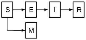
| (18) |
We also consider two important features of disease transmission. First, due to mobility there is contact between infected individuals of one sub-population with the susceptible individuals of another sub-population. Second, due to different levels of mobility between different sub-populations, onset of the pandemic in each of the sub-populations generally vary. Both of these are accounted in the updated states and in eq:(24), where denotes the mobility levels from sub-population to sub-population and corresponds to a sigmoid function, with parameters . In particular, controls the onset of the pandemic in the -th sub-population, therefore we also account for uncertainty in , by appropriately extending the scenario set (for details see SI).
Let , denote the simulation time period, denote the vaccination time-period where are the first and last vaccination days, such that . We can now write the nominal (or non-stochastic) optimization problem (denoted ) for vaccine allocation as (19), where in (19e) denotes the total daily vaccine budget for all sub-populations and in (19f) denotes the vaccine budget for -th sub-population. Equations (19b) represent the ODE constraints, (19c) & (19d) together computes the maximum (or peak) infection of the total population (denoted ) and (19a) minimizes the peak infection.
We now provide the uncertainty-informed, i.e. stochastic counterpart (denoted ) of the nominal problem in (20), where denotes the scenario-set, recall (17). Each state S,E,I,R,M in ODE constraints in (20b) now has an associated superscript corresponding to that scenario, denotes the peak infection for scenario , (20a) computes the expected peak infection over all scenarios. The vaccine budget constrains in (20c) remain same as in .
| (19a) | |||
| s.t. | |||
| (19b) | |||
| (19c) | |||
| (19d) | |||
| (19e) | |||
| (19f) | |||
| (19g) | |||
| (20a) | |||
| (20b) | |||
| (20c) | |||
Definition 5.1.
A vaccine policy is defined as:
Theorem 5.2.
Theorem 5.2 holds true because of the budget constraints (20c), is non-negative and finite. Thus the existence and uniqueness of a solution to ODEs in (20b) is guaranteed and can be shown analytically using the Picard-Lindelöf theorem with appropriate initial conditions [18, 49, 51].
Lemma 5.3.
Decomposability w.r.t : For a given (fixed) vaccine policy , the ODE constraints in (20b) become decomposable, i.e. the set of ODE constraints in scenario can be solved independently of the set of ODE constraints in scenario .
Lemma (5.3) follows from the fact that for a given scenario (say ), constraints in (20b) require parameters only corresponding to scenario . This has major computational implications as it allows for parallel evaluation of scenarios in . Due to the additive nature of the objective function (20a) w.r.t. to , we can compute the objective function value after parallel computation of scenarios. Therefore, we can efficiently solve using an iterative heuristic based optimization procedure described in algorithm 1. Details on heuristics are provided in SI.
6 Experimental (Simulation) Results
We show the efficacy of our proposed approach on two different disease transmission models, i.e. the SEIR and the SEPIHR models. For all experiments we report average of 5 runs. In addition to the experiments in this section, various other numerical experiments under different setups are provided in SI.
Recall that in section 3.1, we have already discussed the details and sampling results for both the SEIR and SEPIHR model including figures 5 & 12 respectively. Also, in section 4 (including fig. 7 & 8), we have discussed how to obtain a tractable scenario set using k-means to account for uncertainty in the vaccine allocation. Therefore our main goal in this section is to show the benefit of incorporating uncertainty by comparing the vaccine allocation policy (denoted ) obtained from solving the nominal formulation against the vaccine allocation policy (denoted ) obtained from solving the stochastic solution . We also benchmark against a zero or no-vaccination policy denoted (denoted ), where .
SEIR model: We use a total simulation time horizon of days, vaccination period of 25 days starting on and ending on with daily available vaccine budgets and . Importantly, note that in section 3.1 for parameter estimation, we used data only for first 15 days, i.e. , thus maintaining consistency for real-world applicability. We perform experiments in two different settings, in the first setting we work with i.e. three sub-populations of sizes respectively and in the second setting we increase to , with an additional sub-population of size . Numerical values of other parameters like and additional experiments to evaluate their effect are provided in SI.
For each setting i.e. and , using algorithm 1 and the nominal estimates of , we solve the to get the nominal vaccine policy . Using the scenario-set (generated from the discrete-parameter distribution) we solve to get the uncertainty-informed vaccine policy .
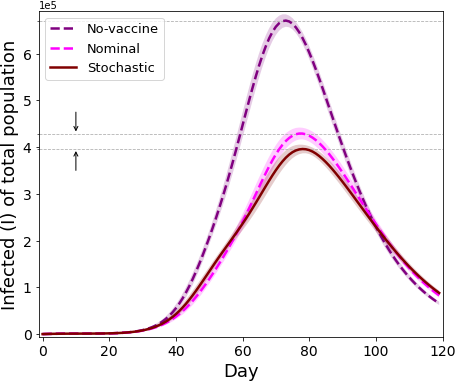
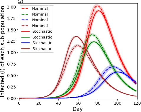
We next evaluate the efficacy of all the three vaccine policies i.e. . For each of these policies, we simulate all the scenarios in the scenario-set and compute the expected values of all the states i.e. S,E,I,R and M over the time horizon .
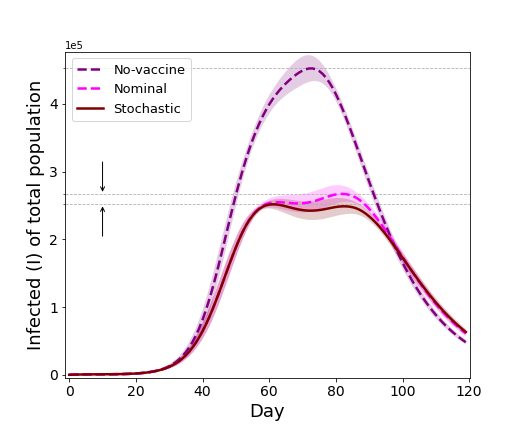
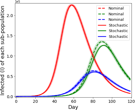
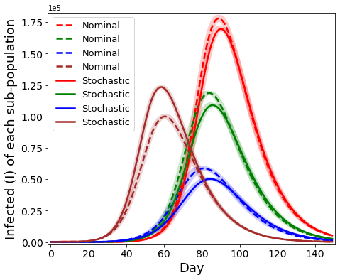
The evolution of the infected state (I) of the total population and the infected (I) and immuned (M) states of each sub-population are shown in fig. 10(a) and 10(b) for and respectively. We note that for (fig 10(a)) , the expected peak infection is reduced from around 501k (with no-vaccination i.e. ) to 324k with nominal vaccination policy . This reduction of peak infection by 35.3% is expected due to vaccination. More importantly, we observe that with the stochastic vaccination policy the peak infection is further reduced to around 308k, which is an improvement of around 4.9% over and 38.56% over . This improvement of over by 4.9% is also referred to as the value of stochastic solution (VSS) or equivalently the benefit of accounting for uncertainty.


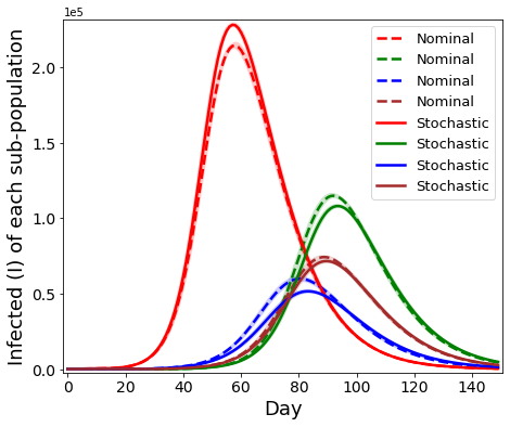
For (fig 10(b)), we observe that the peak infection with no-vaccine policy is around 653k, and is reduced to 393k with and is further reduced to 361k with , i.e. provides a reduction of around 8% over . This higher VSS of 8% for compared to 4.9% for is due to the fact that the size of scenario set is directly proportional to the number of sub-populations . Recall that we also account for the uncertainty in the onset of the pandemic in each sub-population through the parameter .
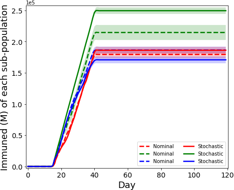
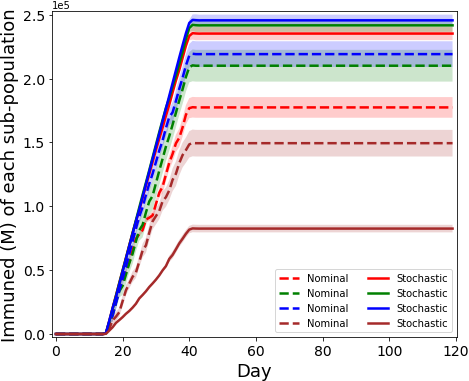
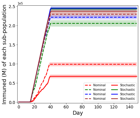
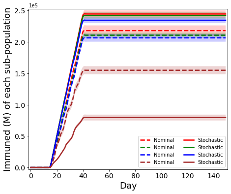
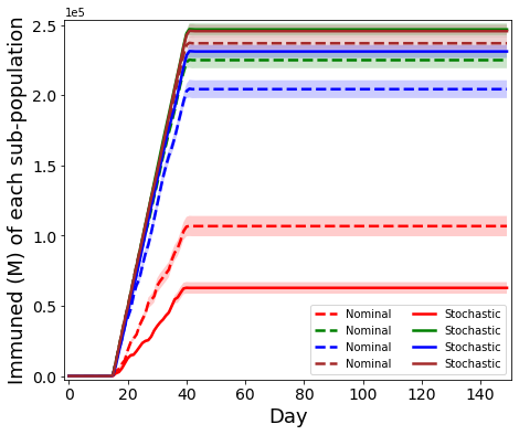
Note that since the immuned sub-population size is directly proportional to vaccines allocated to that sub-population, therefore the third figure in 10(a) and 10(b) also shows how many vaccines are allocated to each sub-population relative to each other. We observe that there is a clear difference between the nominal and the stochastic allocations. This significant difference in nature of the vaccine policies explain the reduction of 4.9% and 8% respectively, providing validity to our results in the sense that the reductions obtained are not simply due to minor numerical changes in solution values. We further discuss the differences of the two policies ( vs ) in SI.
SEPIHR model: We next evaluate our approach on the SEPIHR model with additional states P (for protective quarantine) and H (for hospitalised quarantined). Importantly here as the number of hospitalisations (H) is modeled explicitly, therefore we minimize the peak (maximum) hospitalisations. For this model, corresponding vaccine allocation optimization formulations (i.e. nominal and stochastic) are provided in SI.
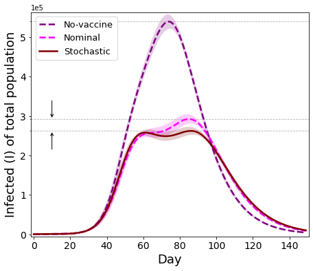
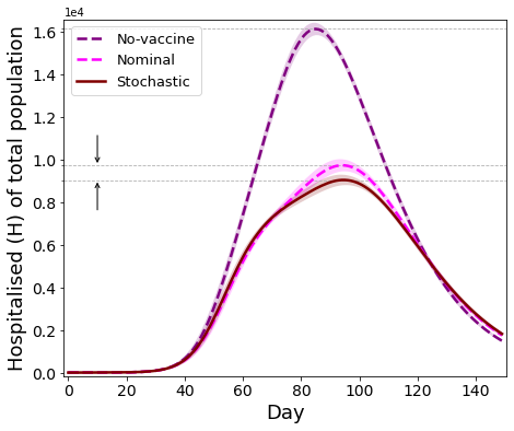
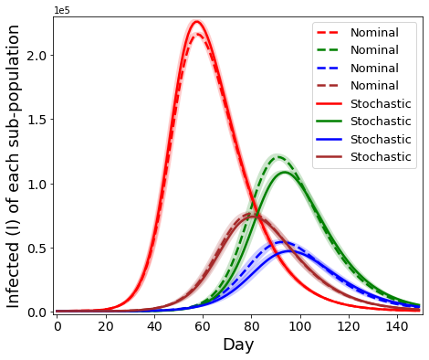
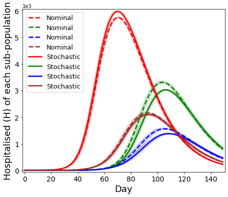
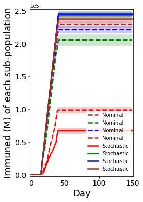
In fig. 11, we show the evolution of the infected (I) and hospitalised (H) states of the total population, along with the I,H and immuned (M) for each of the 4 sub-populations. We note that the peak infections (I) for the three policies (i.e. , and ) are around 539k, 280k and 262k and the peak hospitalisations are around 16k, 9.4k and 9k respectively. Therefore, provides a reduction of 6.3% in peak infections (I) over and a 4.4% reduction in peak hospitalisations (H). Interestingly, from the fifth plot in fig. 10, we note that despite its largest size and earliest the onset of the pandemic, red population is allocated the least vaccines. This can be explained by the fact that we aim to minimize the peak of the total population. In SI, we provide more such sub-population level discussions on the differences in nature the of the optimal policies including vs .
The above results on SEIR and SEPIHR models clearly demonstrate the benefit of uncertainty-informed vaccine allocation using Bayesian inference over using nominal estimates.
Our improvements of 4-8% are either consistent with prior works in literature such as [60] or much better [54].
In SI, we provide more experiments under different setups for both the models. We also discuss the possible societal impact of our work.
7 Concluding Remarks and Future Work
In this paper, we proposed an uncertainty informed vaccine allocation problem as a stochastic optimization problem, for which the tractable scenario-set is constructed in a novel data-driven manner using Bayesian inference for ODEs with GPs. We also proposed a scalable solution algorithm to solve the stochastic program and showed that a significant gain can be achieved by accounting for uncertainty. For future work, a natural extension would be to systematically investigate equity and fairness of allocation through additional constraints and different objective functions.
References
- [1] D. Acemoglu, A. Fallah, A. Giometto, D. Huttenlocher, A. Ozdaglar, F. Parise, and S. Pattathil. Optimal adaptive testing for epidemic control: combining molecular and serology tests, 2021.
- [2] Amani A. Alahmadi, Jennifer A. Flegg, Davis G. Cochrane, Christopher C. Drovandi, and Jonathan M. Keith. A comparison of approximate versus exact techniques for bayesian parameter inference in nonlinear ordinary differential equation models. Royal Society Open Science, 7(3):191315, 2020.
- [3] Daniel Aloise, Amit Deshpande, Pierre Hansen, and Preyas Popat. Np-hardness of euclidean sum-of-squares clustering. Machine Learning, 75:245–248, 2009.
- [4] Anastasios Nikolas Angelopoulos, Reese Pathak, Rohit Varma, and Michael I. Jordan. On identifying and mitigating bias in the estimation of the covid-19 case fatality rate. Harvard Data Science Review, 7 2020. https://hdsr.mitpress.mit.edu/pub/y9vc2u36.
- [5] David Barber and Yali Wang. Gaussian processes for bayesian estimation in ordinary differential equations. In Eric P. Xing and Tony Jebara, editors, Proceedings of the 31st International Conference on Machine Learning, volume 32 of Proceedings of Machine Learning Research, pages 1485–1493, Bejing, China, 22–24 Jun 2014. PMLR.
- [6] NG Becker. The use of mathematical models in determining vaccination policies. Bulletin of the International Statistics Institute, 46:478–490, 1975.
- [7] Dimitris Bertsimas, Joshua Ivanhoe, Alexandre Jacquillat, Michael Li, Alessandro Previero, Omar Skali Lami, and Hamza Tazi Bouardi. Optimizing vaccine allocation to combat the covid-19 pandemic. medRxiv, 2020.
- [8] John R. Birge, Ozan Candogan, and Yiding Feng. Controlling epidemic spread: Reducing economic losses with targeted closures. Management Science, 68(5):3175–3195, 2022.
- [9] Fred Brauer. Compartmental Models in Epidemiology, pages 19–79. Springer Berlin Heidelberg, 2008.
- [10] Fred Brauer. Mathematical epidemiology: Past, present, and future. Infectious Disease Modelling, 2(2):113–127, 2017.
- [11] Suzanne Brøgger. Systems analysis in tuberculosis control: a model. The American review of respiratory disease, 95 3:419–34, 1967.
- [12] Ben Calderhead and Mark Girolami. Estimating bayes factors via thermodynamic integration and population mcmc. Computational Statistics and Data Analysis, 53(12):4028–4045, 2009.
- [13] Ben Calderhead and Mark Girolami. Statistical analysis of nonlinear dynamical systems using differential geometric sampling methods. Interface Focus, 1(6):821–835, 2011.
- [14] Ben Calderhead, Mark Girolami, and Neil Lawrence. Accelerating bayesian inference over nonlinear differential equations with gaussian processes. In D. Koller, D. Schuurmans, Y. Bengio, and L. Bottou, editors, Advances in Neural Information Processing Systems, volume 21. Curran Associates, Inc., 2009.
- [15] Oksana A. Chkrebtii, David A. Campbell, Ben Calderhead, and Mark A. Girolami. Bayesian Solution Uncertainty Quantification for Differential Equations. Bayesian Analysis, 11(4):1239 – 1267, 2016.
- [16] Leonardo Cianfanelli, Francesca Parise, Daron Acemoglu, Giacomo Como, and Asuman Ozdaglar. Lockdown interventions in sir models: Is the reproduction number the right control variable? In 2021 60th IEEE Conference on Decision and Control (CDC), pages 4254–4259, 2021.
- [17] Damian Clancy and Nathan Green. Optimal intervention for an epidemic model under parameter uncertainty. Mathematical biosciences, 205:297–314, 02 2007.
- [18] E. A. Coddington and N. Levinson. Theory of ordinary differential equations. McGraw-Hill New York, 1955.
- [19] Estee Y. Cramer, Evan L. Ray, Velma K. Lopez, Johannes Bracher, Andrea Brennen, Alvaro J. Castro Rivadeneira, …, and Nicholas G. Reich. Evaluation of individual and ensemble probabilistic forecasts of covid-19 mortality in the united states. Proceedings of the National Academy of Sciences, 119(15), 2022.
- [20] Sarat C. Dass, Jaeyong Lee, Kyoungjae Lee, and Jonghun Park. Laplace based approximate posterior inference for differential equation models. Statistics and Computing, 27(3):679–698, may 2017.
- [21] K. Deb, A. Pratap, S. Agarwal, and T. Meyarivan. A fast and elitist multiobjective genetic algorithm: Nsga-ii. IEEE Transactions on Evolutionary Computation, 6(2):182–197, 2002.
- [22] Frank Dondelinger, Dirk Husmeier, Simon Rogers, and Maurizio Filippone. Ode parameter inference using adaptive gradient matching with gaussian processes. In Carlos M. Carvalho and Pradeep Ravikumar, editors, Proceedings of the Sixteenth International Conference on Artificial Intelligence and Statistics, volume 31 of Proceedings of Machine Learning Research, pages 216–228, Scottsdale, Arizona, USA, 29 Apr–01 May 2013. PMLR.
- [23] Chenyi Fu, Melvyn Sim, and Minglong Zhou. Robust epidemiological prediction and optimization. 2021.
- [24] Sanmitra Ghosh, Paul Birrell, and Daniela De Angelis. Variational inference for nonlinear ordinary differential equations. In Arindam Banerjee and Kenji Fukumizu, editors, Proceedings of The 24th International Conference on Artificial Intelligence and Statistics, volume 130 of Proceedings of Machine Learning Research, pages 2719–2727. PMLR, 13–15 Apr 2021.
- [25] Javier González, Ivan Vujačić, and Ernst Wit. Reproducing kernel hilbert space based estimation of systems of ordinary differential equations. Pattern Recognition Letters, 45, 11 2013.
- [26] Nico S Gorbach, Stefan Bauer, and Joachim M Buhmann. Scalable variational inference for dynamical systems. In I. Guyon, U. V. Luxburg, S. Bengio, H. Wallach, R. Fergus, S. Vishwanathan, and R. Garnett, editors, Advances in Neural Information Processing Systems, volume 30. Curran Associates, Inc., 2017.
- [27] Shota Gugushvili and Chris A. J. Klaassen. -consistent parameter estimation for systems of ordinary differential equations: bypassing numerical integration via smoothing. Bernoulli, 18(3):1061–1098, 2012.
- [28] Anthony Hauser, Michel J. Counotte, Charles C. Margossian, Garyfallos Konstantinoudis, Nicola Low, Christian L. Althaus, and Julien Riou. Estimation of sars-cov-2 mortality during the early stages of an epidemic: a modeling study in hubei, china, and six regions in europe. medRxiv, 2020.
- [29] Philipp Hennig, Michael Osborne, and Mark Girolami. Probabilistic numerics and uncertainty in computations. Proceedings of the Royal Society A: Mathematical, Physical and Engineering Science, 471, 06 2015.
- [30] Hanwen Huang, Andreas Handel, and Xiao Song. A bayesian approach to estimate parameters of ordinary differential equation. Computational Statistics, 35, 09 2020.
- [31] S. Hug, A. Raue, J. Hasenauer, J. Bachmann, U. Klingmüller, J. Timmer, and F.J. Theis. High-dimensional bayesian parameter estimation: Case study for a model of jak2/stat5 signaling. Mathematical Biosciences, 246(2):293–304, 2013.
- [32] Hans Kersting, Nicholas Krämer, Martin Schiegg, Christian Daniel, Michael Tiemann, and Philipp Hennig. Differentiable likelihoods for fast inversion of ’likelihood-free’ dynamical systems. In Proceedings of the 37th International Conference on Machine Learning, ICML’20. JMLR.org, 2020.
- [33] Botir Kobilov, Ethan Rouen, and George Serafeim. Predictable country-level bias in the reporting of covid-19 deaths. Journal of Government and Economics, 2:100012, 2021.
- [34] Andrei Kramer, Ben Calderhead, and Nicole Radde. Hamiltonian monte carlo methods for efficient parameter estimation in steady state dynamical systems. BMC bioinformatics, 15:253, 07 2014.
- [35] Michael Lingzhi Li, Hamza Tazi Bouardi, Omar Skali Lami, Thomas A. Trikalinos, Nikolaos Trichakis, and Dimitris Bertsimas. Forecasting covid-19 and analyzing the effect of government interventions. Operations Research, 2022.
- [36] Hua Liang and Hulin Wu. Parameter estimation for differential equation models using a framework of measurement error in regression models. Journal of the American Statistical Association, 103:1570–1583, 12 2008.
- [37] Stuart Lloyd. Least squares quantization in pcm. IEEE transactions on information theory, 28(2):129–137, 1982.
- [38] Benn Macdonald, Catherine Higham, and Dirk Husmeier. Controversy in mechanistic modelling with gaussian processes. In Francis Bach and David Blei, editors, Proceedings of the 32nd International Conference on Machine Learning, volume 37 of Proceedings of Machine Learning Research, pages 1539–1547, Lille, France, 07–09 Jul 2015. PMLR.
- [39] Meena Mahajan, Prajakta Nimbhorkar, and Kasturi Varadarajan. The planar k-means problem is np-hard. In Sandip Das and Ryuhei Uehara, editors, WALCOM: Algorithms and Computation, pages 274–285, Berlin, Heidelberg, 2009. Springer Berlin Heidelberg.
- [40] Guy Mayraz and Geoffrey E Hinton. Recognizing hand-written digits using hierarchical products of experts. In T. Leen, T. Dietterich, and V. Tresp, editors, Advances in Neural Information Processing Systems, volume 13. MIT Press, 2000.
- [41] Mu Niu, Simon Rogers, Maurizio Filippone, and Dirk Husmeier. Fast parameter inference in nonlinear dynamical systems using iterative gradient matching. In Maria Florina Balcan and Kilian Q. Weinberger, editors, Proceedings of The 33rd International Conference on Machine Learning, volume 48 of Proceedings of Machine Learning Research, pages 1699–1707, New York, New York, USA, 20–22 Jun 2016. PMLR.
- [42] Felix Parker, Hamilton Sawczuk, Fardin Ganjkhanloo, Farzin Ahmadi, and Kimia Ghobadi. Optimal resource and demand redistribution for healthcare systems under stress from COVID-19. CoRR, abs/2011.03528, 2020.
- [43] L. Mihaela Paun and Dirk Husmeier. Emulation-accelerated hamiltonian monte carlo algorithms for parameter estimation and uncertainty quantification in differential equation models. Statistics and Computing, 32(1), feb 2022.
- [44] J. O. Ramsay, G. Hooker, D. Campbell, and J. Cao. Parameter estimation for differential equations: a generalized smoothing approach. Journal of the Royal Statistical Society: Series B (Statistical Methodology), 69(5):741–796, 2007.
- [45] Carl Edward Rasmussen. Gaussian processes for machine learning. MIT Press, 2006.
- [46] Geoffrey Roeder, Paul Grant, Andrew Phillips, Neil Dalchau, and Edward Meeds. Efficient amortised Bayesian inference for hierarchical and nonlinear dynamical systems. In Kamalika Chaudhuri and Ruslan Salakhutdinov, editors, Proceedings of the 36th International Conference on Machine Learning, volume 97 of Proceedings of Machine Learning Research, pages 4445–4455. PMLR, 09–15 Jun 2019.
- [47] G. Rohith. An augmented seir model with protective and hospital quarantine dynamics for the control of covid-19 spread. medRxiv, 2021.
- [48] Napat Rujeerapaiboon, Kilian Schindler, Daniel Kuhn, and Wolfram Wiesemann. Scenario reduction revisited: fundamental limits and guarantees. Mathematical Programming, 191:207–242, 2022.
- [49] S. Sastry. Nonlinear Systems: Analysis, Stability, and Control. Interdisciplinary Applied Mathematics. Springer New York, 2013.
- [50] E. Solak, R. Murray-smith, W. Leithead, D. Leith, and Carl Rasmussen. Derivative observations in gaussian process models of dynamic systems. In S. Becker, S. Thrun, and K. Obermayer, editors, Advances in Neural Information Processing Systems, volume 15. MIT Press, 2002.
- [51] Samuel Sowole, Daouda Sangare, Abdullahi Ibrahim, and Isaac Paul. On the existence, uniqueness, stability of solution and numerical simulations of a mathematical model for measles disease. 2019:84–111, 07 2019.
- [52] Matthew Tanner, Lisa Sattenspiel, and Lewis Ntaimo. Finding optimal vaccination strategies under parameter uncertainty using stochastic programming. Mathematical biosciences, 215:144–51, 08 2008.
- [53] Onur Teymur, Ben Calderhead, Han Cheng Lie, and T. J. Sullivan. Implicit probabilistic integrators for odes. In Proceedings of the 32nd International Conference on Neural Information Processing Systems, NIPS’18, page 7255–7264, Red Hook, NY, USA, 2018. Curran Associates Inc.
- [54] Lawrence Thul and Warren Powell. Stochastic optimization for vaccine and testing kit allocation for the covid-19 pandemic. European Journal of Operational Research, 304(1):325–338, 2023. The role of Operational Research in future epidemics/ pandemics.
- [55] Tina Toni, David Welch, Natalja Strelkowa, Andreas Ipsen, and Michael Stumpf. Approximate bayesian computation scheme for parameter inference and model selection in dynamical systems. j r soc interface 6: 187-202. Journal of the Royal Society, Interface / the Royal Society, 6:187–202, 03 2009.
- [56] Filip Tronarp, Nathanael Bosch, and Philipp Hennig. Fenrir: Physics-enhanced regression for initial value problems, 2022.
- [57] J. Vanlier, C.A. Tiemann, P.A.J. Hilbers, and N.A.W. van Riel. Parameter uncertainty in biochemical models described by ordinary differential equations. Mathematical Biosciences, 246(2):305–314, 2013.
- [58] Philippe Wenk, Gabriele Abbati, Michael Osborne, Bernhard Schölkopf, Andreas Krause, and Stefan Bauer. Odin: Ode-informed regression for parameter and state inference in time-continuous dynamical systems. Proceedings of the AAAI Conference on Artificial Intelligence, 34:6364–6371, 04 2020.
- [59] Philippe Wenk, Alkis Gotovos, Stefan Bauer, Nico S. Gorbach, Andreas Krause, and Joachim M. Buhmann. Fast gaussian process based gradient matching for parameter identification in systems of nonlinear odes. In Kamalika Chaudhuri and Masashi Sugiyama, editors, Proceedings of the Twenty-Second International Conference on Artificial Intelligence and Statistics, volume 89 of Proceedings of Machine Learning Research, pages 1351–1360. PMLR, 16–18 Apr 2019.
- [60] Hamed Yarmand, Julie S. Ivy, Brian Denton, and Alun L. Lloyd. Optimal two-phase vaccine allocation to geographically different regions under uncertainty. European Journal of Operational Research, 233(1):208–219, 2014.
- [61] Xuecheng Yin and I. Esra Buyuktahtakin. A multi-stage stochastic programming approach to epidemic resource allocation with equity considerations. Health Care Management Science, 2021.
- [62] Xuecheng Yin, I. Esra Buyuktahtakin, and Bhumi P. Patel. Covid-19: Data-driven optimal allocation of ventilator supply under uncertainty and risk. European Journal of Operational Research, 304(1):255–275, 2023.
Supplementary Information (SI)
1 Societal Impact
Previous studies [7, 1, 8, 42] have shown that accurate and data-informed modeling of the spread of a pandemic is extremely useful for policy makers and public health agencies to make time-sensitive critical decisions. These decisions generally include imposing lockdowns, allocation of resources such as medical personnel, medical supplies (PPE kits, masks, oxygen etc.), testing facilities and vaccines. Needless to mention that public health and economic recovery of our society crucially depends on these decisions.
Our approach and results suggest that accounting for uncertainty in key epidemiological parameters can improve the efficacy of time-critical allocation decisions. We believe that our work will mainly have a positive societal impact. However, at the same time it is extremely important to be mindful of the fairness and equity aspects of resource allocation. Given the flexible nature of our approach, we believe that our work can be leveraged to study and address these aspects systematically.
2 Definition of
Let denote the a valid kernel function, then the entries of the matrices i.e. are given as:
3 GP hyper-parameter estimation
For a zero-mean Gaussian process (), with hyper-parameters and , the log-likelihood of observations (denoted y) at evaluation times t can be obtained in closed form as [45]:
| (21) |
Equation (21) can be maximized w.r.t to and . Note that the equation does not depend on the functional form of the ODEs.
4 Accounting for uncertainty in
The value of the parameter controls the onset of the pandemic in the -th sub-population. We therefore also account for the uncertainty in the onset on the pandemic in each of the sub-populations. We do this by augmenting the different scenarios in the scenario set . For each sub-population we consider different values of , where is around 4-5. Let , then
, or equivalently we can write:
and
Using , we get the final scenario set as , where is the scenario set obtained after running k-means on the discrete parameter distribution. The probabilities of different scenarios in can be obtained easily by adjusting the probabilities of scenarios in by a factor of .
5 Numerical Values of different parameters
For the experiments in the main text we used the following values:
We use and .
We use the following base mobility matrices depending on the number of sub-populations:
is equal to the entry of , i.e. .
5.1 SEIR model
For , we used
and the base mobility matrix with .
and .
For we used
and the base mobility matrix .
and .
5.2 SEPIHR model
We used a total simulation time horizon of days, vaccination period of 25 days starting on and ending on .
We used and the base mobility matrix with .
and .
6 Sampling Details
6.1 SEIR model
In the sampling, we used the following upper and lower bounds on respectively :
We ran the sampling algorithm for a total of k iterations, from which we discard the first k samples as burn-in [59].
6.2 SEPIHR model
We use as the true parameter values. We simulate an SEPIHR model (eq:(22)) to get state values. We add zero-mean Gaussian noise with to each of the simulated state values to generate our dataset. Using this data only for 15 days (), we first estimate the GP hyper-parameters for states using maximum-likelihood (see (21)).
We then run the Metropolis-Hastings MCMC sampling procedure to get our empirical posterior joint-distribution on . Note that as discussed earlier in section 10, we keep fixed, as these are known clinical parameters.
We use the following upper and lower bounds:
After removing the burn-in samples, for the remaining samples, we plot the marginal distributions along with their mean and mode in fig. 12. Mode is a more representative statistic here as the distributions are not symmetric due to non-negative support.

7 Discussion on the resulting optimal vaccine policies
In this section we discuss the resulting optimal vaccine policies i.e. nominal and stochastic policies for the three set of experiments in the main text.
7.1 SEIR model


For , we note from fig. 13(a), that under the nominal policy, least number of vaccines are allocated to the blue sub-population even though the onset of the pandemic is first in this sub-population. Interestingly, even though the red sub-population is larger than the green sub-population, however, slightly more vaccines are allocated to the green sub-population in comparison to the red sub-population.
Under the stochastic policy, in the face of uncertainty, even fewer vaccines are allocated to the blue sub-population and proportionally more vaccine are allocated to red and blue sub-populations.
For , we note from fig. 13(b), that under the nominal policy, both the brown and the red sub-populations are allocated similar number of total vaccines despite the difference in their population size and the onset of the pandemic. Interestingly, even though the blue sub-population size is much smaller, however, it is allocated larger number of total vaccines in comparison to both the red and brown sub-populations.
Under the stochastic policy, the brown sub-population receives even fewer vaccines and proportionally more vaccines are allocated to the other three sub-populations.
7.2 SEPIHR model


We note from fig. 14, that under the nominal policy, least number of vaccines are allocated to the red sub-population regardless of its large size and the fact that the onset of the pandemic is first in this sub-population. This at first glance seems to be counter-intuitive, however can be explained by the fact that we aim to minimize the peak hospitalizations of the total population which occurs around 82nd day. Further, despite the the brown and the blue sub-populations being smallest in size, receive larger number of vaccines. Under the stochastic policy even fewer vaccines are allocated to red sub-population and correspondingly more vaccines are allocate to the other three sub-populations. Importantly, also note that due to vaccination (both in the nominal and stochastic case) the peak of both the infections and hospitalisations is delayed in comparison to no-vaccination case, thus further alleviating the burden of the medical personnel.
8 Additional experiments for SEIR model with sub-populations
Evaluation of different vaccination policies i.e. no-vaccine policy , nominal policy and stochastic policy under different scenarios of and mobility matrix M.
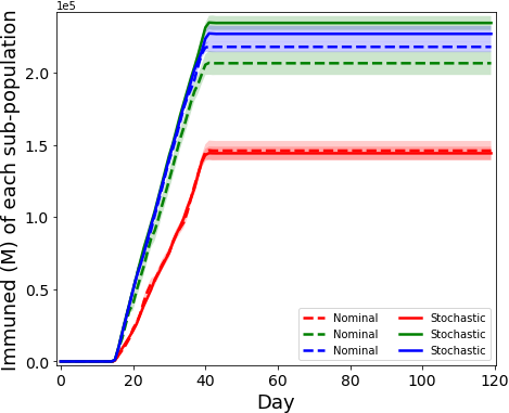
Setup: and mobility matrix with and .
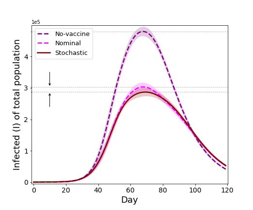
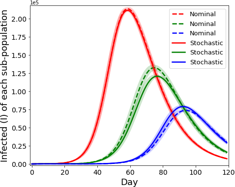
Setup: and mobility matrix with and .
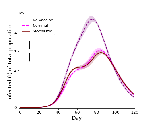
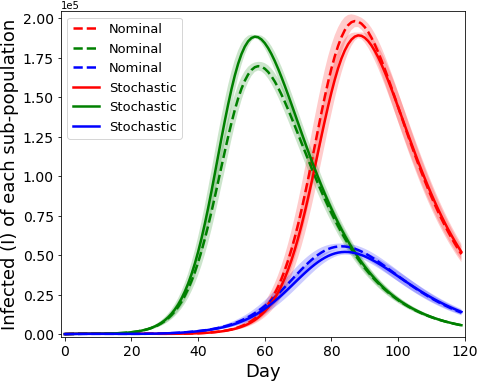
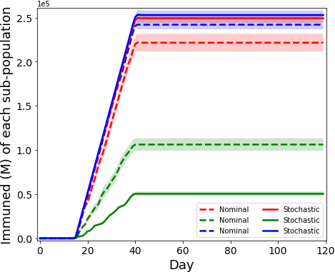
Setup: and mobility matrix with and .
9 Additional experiments for SEIR model with sub-populations
Evaluation of different vaccination policies i.e. no-vaccine policy , nominal policy and stochastic policy under different scenarios of and mobility matrix M.
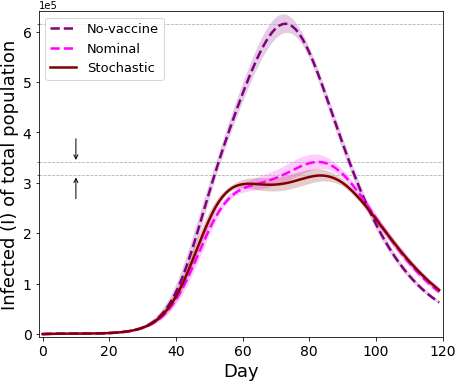
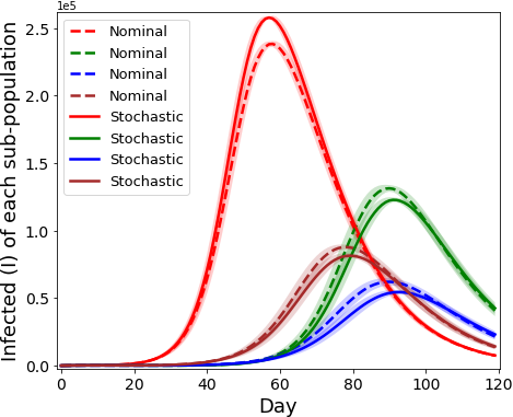
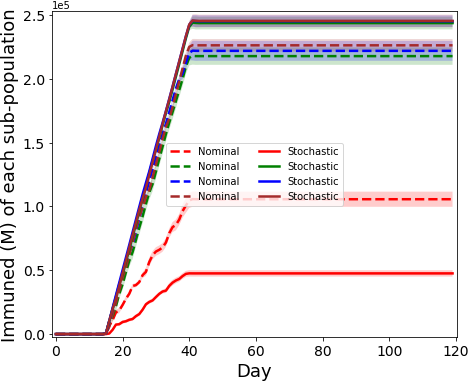
Setup: and mobility matrix with and .
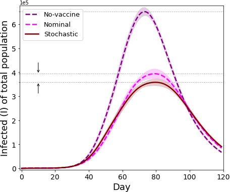
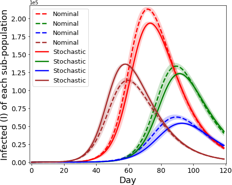
Setup: and mobility matrix with and .
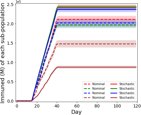
Setup: and mobility matrix .
10 SEPIHR model details & Nominal and Stochastic optimization problem formulations
We mathematically describe the ODEs governing the evolution of each of the states in the SEPIHR disease transmission model shown in fig. 21 in equations (22).
(22a)
(22b)
(22c)
(22d)
(22e)
(22f)
![[Uncaptioned image]](/html/2307.00032/assets/img/SEPIHR_compact.png) Figure 21: SEPIHR model.
The SEPIHR model (22) has two set of parameters, where in the first set we have and in the second set we have . Parameters in the second set, also referred to as clinical parameters, i.e. and are the rates at which a quarantined person is hospitalised, an infected person is hospitalised and the rate at which a hospitalised person leaves the hospital respectively. These rates (i.e. second set of parameters) have standard values [7], for instance a person on an average would spend 15-16 days in the hospital, therefore . Importantly, accurately estimating these clinical parameters require data which is typically only available to hospitals and medical personnel. Therefore we prefer to use the standard known values for these parameters instead of estimating them from daily counts data. We use as the true parameter values.
Additionally, this also helps to keep the sampling space small (i.e. 5 dimensional), therefore MCMC sampling remains computationally tractable as we only estimate the posterior joint distribution over the first set of parameters, i.e. . For sampling details, refer to section 6.2.
Figure 21: SEPIHR model.
The SEPIHR model (22) has two set of parameters, where in the first set we have and in the second set we have . Parameters in the second set, also referred to as clinical parameters, i.e. and are the rates at which a quarantined person is hospitalised, an infected person is hospitalised and the rate at which a hospitalised person leaves the hospital respectively. These rates (i.e. second set of parameters) have standard values [7], for instance a person on an average would spend 15-16 days in the hospital, therefore . Importantly, accurately estimating these clinical parameters require data which is typically only available to hospitals and medical personnel. Therefore we prefer to use the standard known values for these parameters instead of estimating them from daily counts data. We use as the true parameter values.
Additionally, this also helps to keep the sampling space small (i.e. 5 dimensional), therefore MCMC sampling remains computationally tractable as we only estimate the posterior joint distribution over the first set of parameters, i.e. . For sampling details, refer to section 6.2.
The spread of disease in each of the -th sub-population, where , is modeled using a separate SEPIHR model.
To account for the vaccinated individuals, the SEPIHR model in fig. 21 is updated with a new compartment (denoted by M) to represent the immune population and the updated model shown in fig. 22, is denoted as the SEPIHRM model. Let represent the number of people vaccinated at time in the -th sub-population and be efficacy of the vaccine, then the ODEs corresponding to the SEIRM model of the -th sub-population are given as:
(23a)
(23b)
(23c)
(23d)
(23e)
(23f)
(23g)
![[Uncaptioned image]](/html/2307.00032/assets/img/SEPIHRM_compact.png) Figure 22: SEPIHRM model.
We consider two important features of disease transmission. First, due to mobility there is contact between infected individuals of one sub-population with the susceptible individuals of another sub-population. Second, due to different levels of mobility between different sub-populations,
onset of the pandemic in each of the sub-populations generally vary. Both of these are accounted by updating the states and as follows:
(24a)
(24b)
Figure 22: SEPIHRM model.
We consider two important features of disease transmission. First, due to mobility there is contact between infected individuals of one sub-population with the susceptible individuals of another sub-population. Second, due to different levels of mobility between different sub-populations,
onset of the pandemic in each of the sub-populations generally vary. Both of these are accounted by updating the states and as follows:
(24a)
(24b)
where denotes the mobility levels from sub-population to sub-population and corresponds to a sigmoid function, with parameters . In particular, controls the onset of the pandemic in the -th sub-population, therefore we also account for uncertainty in , by appropriately extending the scenario set . We can now write the corresponding nominal (or non-stochastic) optimization problem (denoted ) for vaccine allocation as follows: (25a) s.t. (25b) (25c) (25d) (25e) (25f) (25g)
where denotes the daily total vaccination budget and denotes the daily vaccination budget of the -th sub-population. Note that in the above formulations, we are minimizing peak hospitalizations. We next provide the uncertainty-informed, i.e. stochastic counterpart (denoted ) of the above nominal problem .
| (26a) | ||||
| s.t. | ||||
| (26b) | ||||
| (26c) | ||||
11 Additional experiments for SEPIHR model with sub populations
![[Uncaptioned image]](/html/2307.00032/assets/img/icml_figs_SEQIHR_pop_4_exps/rank_1_infected_total_I.png)
![[Uncaptioned image]](/html/2307.00032/assets/img/icml_figs_SEQIHR_pop_4_exps/rank_1_infected_total_H.png)

Setup: and mobility matrix with and .
![[Uncaptioned image]](/html/2307.00032/assets/img/icml_figs_SEQIHR_pop_4_exps/rank_1_pop_individual_H.png)
![[Uncaptioned image]](/html/2307.00032/assets/img/icml_figs_SEQIHR_pop_4_exps/rank_12_infected_total_I.png)
![[Uncaptioned image]](/html/2307.00032/assets/img/icml_figs_SEQIHR_pop_4_exps/rank_12_infected_total_H.png)
Setup: and mobility matrix with and .
![[Uncaptioned image]](/html/2307.00032/assets/img/icml_figs_SEQIHR_pop_4_exps/rank_12_pop_individual_H.png)
![[Uncaptioned image]](/html/2307.00032/assets/img/icml_figs_SEQIHR_pop_4_exps/rank_9_infected_total_I.png)
![[Uncaptioned image]](/html/2307.00032/assets/img/icml_figs_SEQIHR_pop_4_exps/rank_9_infected_total_H.png)
Setup: and mobility matrix with and .
![[Uncaptioned image]](/html/2307.00032/assets/img/icml_figs_SEQIHR_pop_4_exps/rank_9_pop_individual_H.png)
12 Product of Experts (PoE) approach
[TextFont= ]
A Gaussian process (GP) prior is placed on , with and as the hyper-parameters of this GP with kernel matrix , we can then write:
| (27) |
Using the Gaussian process defined on the state variables , we can also make predictions about their derivatives as and are jointly Gaussian distributed. We can write the conditional distribution of the state derivatives as :
| (28) |
Note that corresponds to the second, i.e. GP part of the graphical model in fig. 27.
Using the functional form of the ODEs and with state specific Gaussian additive noise , we can write
| (29) |
where . Note that (29), corresponds to the ODE part of the graphical model in the fig. 27. The two models in (28) and in (29) are now combined using a product of experts (PoE) approach [40].
The use of PoE to combine the two models (see fig. 27) was originally proposed by [14] and also used by [22]. In the PoE approach the two models are combined to get the distribution of as follows:
| (30) |
The joint distribution can be derived as follows:
| (31) |
where are the prior distributions on ODE parameters , Kernel hyper-parameters and error term respectively. Note that controls the tightness of the gradient coupling.
In (31), after substituting with (30) and with (27) we get
| (32) |
In (32), marginalization over results in the following:
| (33) | ||||
| (34) |
Note that and since the integral in (34) is analytically tractable, we get:
| (35) |
where denotes . The joint probability for the whole system is given as:
| (36) |
Note that the first factor in (36) is defined in the main text and the second factor is defined in (35). Finally, [22] developed a Metropolis-Hastings based sampling scheme to sample directly from the posterior distribution .
In summary, the use of PoE heuristics in literature is common. Both [14] and [22] using PoE were able to good estimates for using MCMC sampling procedures.
Furthermore, [26] also using PoE in a Variational inference setting reported a better performance both in terms of computation time and quite surprisingly also in the solution quality, despite their Variational inference setting. The surprising improvement of [26] over [14] and [22] indicated that even though solution approaches developed using PoE as an intermediary step seems to be working empirically, however there is some discrepancy in the overall system. This discrepancy was identified, explained and corrected by [59]. \SetVertexStyle[TextFont= ]
Authors in [59] noted that after the marginalization of , the PoE graphical model results in the graphical model shown in 28. In this graphical model there is no link between the parameters and the observations y, thus defeating the whole purpose of combining the ODE model and GP model (in figure 27) using PoE. Due to this discrepancy, we used the alternative graphical model proposed by [59] to estimate the posterior-distribution on ODE parameters..
13 Details on Heuristics
In Algorithm 1, we use a genetic-algorithm (GA) [21] as the heuristic to generate the new batch of policies (of size ) in step 8, using the objective function values and constraint violations of the current batch.
We briefly provide the different steps involved in the working of the GA:
-
1.
The algorithm starts by randomly generating a set of solutions (also referred as individuals) collectively known as the initial population or parent population of size B.
-
2.
The B solutions in the parent population are then evaluated (preferably in parallel), i.e. the objective function values and constraint violations are computed for each of these individuals.
-
3.
The individuals in the parent population are then ranked based on a criteria which depends on the objective function value and the amount of constraint violation.
-
4.
From the B solutions in the parent population another set of B solutions (or individuals) are generated using genetic operators i.e. SBX crossover and polynomial mutation. The new set of B solutions are collectively known as the child population.
-
5.
The child population is then evaluated (preferably in parallel) i.e. their objective function values and constraint violations are computed.
-
6.
The child population and the parent population are then simply merged to form a single population of size 2B known as the mixed population.
-
7.
The individuals in the mixed population are then assigned a rank based on the ranking criteria. Out of the 2B individual in the mixed population, top B ranking individuals are selected and these selected individuals form the parent population for the next iteration. If the termination criteria (typically a max. number of iterations) is not met, then repeat from step 3.
For exact mathematical details on different operators like SBX crossover, polynominal mutation and the ranking criteria we refer the reader to the original paper [21]. Also, the source code for this GA can be easily obtained from the author’s website.
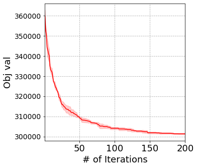
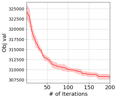
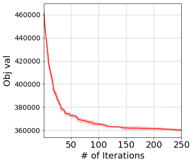
Following are the values of the different hyper-parameter involved in the GA: population size (B) = 100, probability of cross-over = 0.9, probability of mutation = 0.5, distribution index for SBX crossover () = 10, distribution index for real variable polynomial mutation () = 10. For the experiments when , we used a maximum of 200 iterations and when , we used a maximum of 250 iterations.
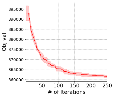
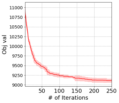
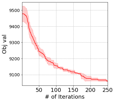
14 Convergence of Algorithm 1
Convergence of Algorithm 1 on Nominal and Stochastic optimization problems for different experiments in the main text. We report mean and standard deviation of 5 runs.
15 Computational resources
Our approach consists of the following computational components: i) MCMC sampling, ii) Tractable scenario-set construction with k-means clustering, iii) Solving the nominal vaccine allocation optimization problem and iv) Solving the stochastic vaccine allocation optimization problem. For the first three components, we run all our experiments on a computer (desktop) with Intel Core i7-6800K CPU with 12 cores and 64GB RAM. For the last component, we run all our experiments on a single server node with Intel(R) Xeon(R) Platinum 8260 CPU with 96 cores and 128 GB RAM.
16 Tractable scenario-set construction: Effect of changing k
16.1 SEIR model


16.2 SEPIHR model


