Domain Wall interpretation of PTA signal confronting Black Hole overproduction

Abstract

Recently, Pulsar Timing Array (PTA) collaborations have detected a stochastic gravitational wave background (SGWB) at nano-Hz frequencies, with Domain Wall networks (DWs) proposed as potential sources. To be cosmologically viable, they must annihilate before dominating the universe energy budget, thus generating a SGWB. While sub-horizon DWs shrink and decay rapidly, causality requires DWs with super-horizon size to continue growing until they reach the Hubble horizon. Those entering the latest can be heavier than a Hubble patch and collapse into Primordial Black Holes (PBHs). By applying percolation theory, we pioneer an estimation of the PBH abundance originating from DW networks. We conduct a Bayesian analysis of the PTA signal, interpreting it as an outcome of SGWB from DW networks, accounting for PBH overproduction as a prior. We included contributions from supermassive black hole binaries along with their astrophysical priors. Our findings indicate that DWs, as the proposed source of the PTA signal, result in the production of PBHs about ten times heavier than the sun. The binary mergers occurring within these PBHs generate a second SGWB in the kilo-Hz domain which could be observable in on-going or planned Earth-based interferometers if the correlation length of the DW network is greater than approximately 60$\%$ than the cosmic horizon, $L\gtrsim 0.6t$.

I.   INTRODUCTION

NANOGrav 15-year (NG15) [1], EPTA [2], PPTA [3], CPTA [4], summarized in [5], have recently reported the observation of a nano-Hz stochastic gravitational wave background (SGWB) [1], confirming the hint observed in previous years [6, 7, 8, 9]. Sources of nano-Hz GWs could be a population of supermassive black hole binaries (SMBH) [10, 11, 12, 13, 14] or could be related to early universe phenomena [15, 16], such as phase transitions [17, 18, 19, 20, 21], large inhomogeneities [22, 23, 24, 25, 26, 27, 28], topological defects [29, 30, 31, 32, 33, 34, 35], and PBHs mergers [36, 37].

Domains Walls are topological defects forming after the spontaneous breaking of a discrete symmetry, e.g. $\mathcal{Z}_{2}$ [38, 39, 40, 41]. DWs dilute slower than radiation in expanding cosmology [42, 43]. To be viable, there must exist an energy bias between distinct vacua so that DWs are pulled toward annihilating with each other. Upon annihilating around QCD confinement epoch, DW networks can produce a SGWB [44, 45, 46, 47, 41] with a nano-Hz peak frequency detectable by PTAs [48]. DW networks feature closed domains configuration which collapse to PBHs when they shrink below their Schwarzschild radius [49, 50, 51] in a process dubbed “catastrogenesis” [52, 53].

In this letter, we report important advances in our comprehension of PBH formation during the annihilation of long-lived DWs networks, with the details deferred to a companion paper [51]. Our work bridges the gap in understanding that was present in previous studies [49, 52, 53]. Our results indicate that the DWs which collapse into PBHs are those that are super-horizon at the beginning of the annihilation phase, and their abundance can be estimated in percolation theory. Performing Bayesian analysis of PTA datasets NG15 [1] and IPTA2 [9], we find that DW networks, possibly combined with SMBH binaries, can not only be a plausible source of the observed PTA signal, but can also lead to the production of PBHs in quantities that can be probed using kilo-Hz interferometers, astrometric measurements, and 21-cm line observations.

Figure 1: LEFT: SGWB from DW network annihilation (solid) preferred by PTA datasets, assuming annihilation into SM radiation and neglecting the PBH prior constraints. In (dotted), we show the preferred SGWB from SMBH binaries, assuming the astrophysical prior drawn from the ${\tt GWOnly-Ext}$ library [15], whose $68\%$ and $90\%$ confidence levels are depicted with the gray bands. We refer to Table 2 for the mean posterior values. RIGHT: With orange and blue ellipses, we show the $68\%$ and $90\%$ confidence levels of the DW interpretation of the PTA signal, assuming SM reheating and neglecting PBH prior constraints. The dashed brown region shows the PBH abundance given in Eq. (13) assuming a DW network correlation length $L/t=0.8$, which might be a conservative choice, see below Eq. (1). We show the associated PBH bounds from on-going kilo-Hz GW interferometers [54, 55, 56, 57, 58] (blue) and CMB [59, 60, 61] (yellow). Part of the DW interpretation is in tension with PBH overproduction constraints. In dashed purple, we show the BBN bound $N_{\rm eff}\lesssim 0.4$ which only applies if the DW network annihilate entirely into dark degrees of freedom. In dotted gray, we show the region when the bias energy density $V_{\rm bias}$ locally dominates the energy density of the universe. We refer to App. B for more details the DW network interpretation of PTA signal.

II.   GRAVITATIONAL WAVES

Annihilating DW networks – After a phase of friction-domination whose duration is model dependent [62], numerical simulations have shown that the energy stored in DWs reaches the scaling regime [43, 40]:

$$\rho_{\rm DW}=\frac{\sigma}{L},\qquad\textrm{with}\leavevmode\nobreak\ L\simeq t/\mathcal{A},$$ (1)

where $L$ is the typical correlation length of the DW network. Numerical simulations of the $\mathcal{Z}_{2}$-model have found $\mathcal{A}\simeq 0.8\pm 0.1$ [47], leading to $L/t=1.25^{+0.18}_{-0.14}$. Other simulations found $L/t\simeq 1.14\pm 0.04$ [63]. Eq. (1) results in the DW energy density redshifting slower than the main radiation fluid $\rho_{\rm rad}\simeq\pi^{2}g_{*}T^{4}/30\propto 1/t^{2}$ such that DWs dominate the energy density of the universe after the time:

$$t_{\rm dom}^{{\rm unbias}}\leavevmode\nobreak\ =\leavevmode\nobreak\ \frac{3M_{\rm pl}^{2}}{4\mathcal{A}\sigma}.$$ (2)

We assume the presence of high dimensional operators that explicitly break $U(1)$ symmetry [64, 38, 65, 66]. This transforms the flat direction into a discrete collection of vacua. DWs annihilate when the vacuum pressure $V_{\rm bias}$ between these new minimum points surpasses the pressure $C_{d}\,\sigma/L$ arising from their surface tension $\sigma$, after the time:

$$t_{\rm ann}\leavevmode\nobreak\ \simeq\leavevmode\nobreak\ C_{d}\,\mathcal{A}\,\frac{\sigma}{V_{\rm bias}},$$ (3)

where $C_{d}\simeq\rm a\leavevmode\nobreak\ few$ can be inferred from numerical simulations [67]. We take $C_{d}\simeq 3$. To be viable, DW must annihilate before the energy bias dominate the energy density $3M_{\rm pl}^{2}H^{2}\simeq V_{\rm bias}$ of the universe at time:

$$t_{\rm dom}\leavevmode\nobreak\ \simeq\leavevmode\nobreak\ \frac{\sqrt{3}M_{\rm pl}}{2\sqrt{V_{\rm bias}}}.$$ (4)

We introduce the DW energy fraction of the universe at $t_{\rm ann}$:

$$\alpha_{\rm ann}\equiv\frac{\rho_{\rm DW}}{3M_{\rm pl}^{2}H^{2}}\Big{|}_{t=t_{\rm ann}}\simeq\left(\frac{t_{\rm ann}}{t_{\rm dom}^{{\rm unbias}}}\right)\simeq C_{d}^{-1}\left(\frac{t_{\rm ann}}{t_{\rm dom}}\right)^{2},$$ (5)

where we approximated $H\simeq 1/2t$ valid for radiation-dominated universe. During the annihilation process, DWs are driven to relativistic speed and radiate GWs [38, 39, 68, 44], leading to the power spectrum today [45, 46, 47]:

$$\Omega_{\rm GW}h^{2}=\mathcal{D}\frac{3}{32\pi}\epsilon_{{\rm GW}}\alpha_{\rm ann}^{2}S(f),$$ (6)

where $\mathcal{D}\sim 10^{-5}$ accounts for redshift, $S(f)$ is a spectral function peaked at $f_{\rm peak}\sim{\rm nHz}\left({T_{\rm ann}/10\leavevmode\nobreak\ \rm MeV}\right)$ and $\epsilon_{{\rm GW}}=\epsilon_{{\rm GW}}=0.7\pm 0.4$ is fitted against numerical simulation [47]. We defer the details concerning the SGWB to App. B.

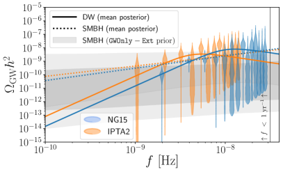
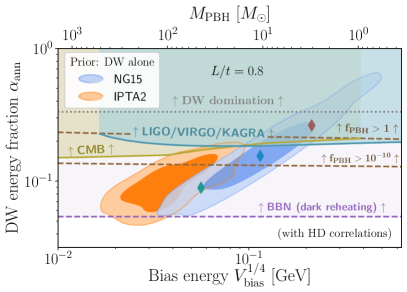
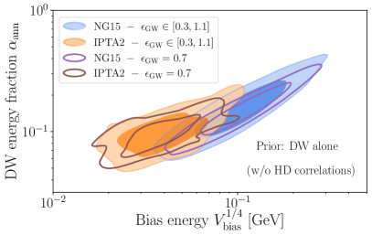
Bayesian analysis – We used the software tool ${\tt PTArcade}$ [69] to conduct a series of Bayesian analysis of the interpretation of PTA signal as resulting from DW networks, SMBH binaries or a combination of them. We used the first $14$ frequency bins of NG15 [6] and the first 13 frequency bins of IPTA2 [9]. We use the mode “enterprise” of PTArcade with $5\times 10^{5}$ steps, including Helling-Down inter-pulsar correlations, see App. A for the details. The favored SGWB and model posteriors of the DW interpretation are visible in Fig. 1, under the assumption of DW annihilation into Standard Model (SM) and not including PBHs constraints as a prior. We report the DW+SMBH interpretation to App. C. The Bayes factors and mean values for the model parameters, encompassing a wide range of priors, are reported in Tabs. 1 and 2.

III.   PBH FORMATION

Domain wall late-annihilation mechanism — DW networks have close configurations that are filled with the energy density $V_{\rm bias}$. Approximating DWs as spherical objects, their mass-energy is given by [70, 71, 72]:

$$M=M_{\rm bulk}+M_{\rm bdy}+M_{\rm bind},$$ (7)

where $M_{\rm bulk}=4\pi V_{\rm bias}R^{3}/3$ is a volume term, $M_{\rm bdy}=4\pi\sigma\gamma R^{2}$ is a boundary term, and $M_{\rm bind}\simeq-8\pi^{2}G\sigma^{2}R^{3}$ is the repulsive surface-surface gravitational binding energy. Close DWs collapse into PBHs when they enter their Schwarzschild radius at a time $t_{\rm PBH}$:

$$R(t_{\rm PBH})=2GM(t_{\rm PBH}).$$ (8)

Assuming that DWs collapse within one light-crossing time, we can replace $R(t_{\rm PBH})\simeq t_{\rm PBH}$ in Eq. (8). Approximating $M\simeq M_{\rm bulk}$, leads to $t_{\rm PBH}=2t_{\rm dom}$. However, the bulk term only accounts for $25\%$ of the DW mass. Accounting for the surface ($50\%$) and binding energy ($25\%$), we find that PBHs form twice lighter, half a cosmic time earlier, at [51]:

$$t_{\rm PBH}\simeq t_{\rm dom}.$$ (9)

This enhances the PBH abundance by many orders of magnitude, leading the lower limit on $\alpha_{\rm ann}$ from PBH overproduction to be stronger by a factor $\sim 4$. Such difference is crucial to investigate PBH production within the PTA posterior region. The equation of motion (EoM) of a bubble of false vacuum in the thin-shell limit in General Relativity has been studied by many authors [73, 74, 75, 76, 77, 70, 71, 72]. By solving the EoM, we obtain that spherical DWs enter their Schwarzschild radius at $t_{\rm PBH}$ if they have a radius equal to [51]:

$$\frac{R_{\rm ann}^{\rm PBH}}{t_{\rm ann}}\simeq 0.780\,{\rm Log_{10}^{2}}\left(\alpha_{\rm ann}\right)-0.618\,{\rm Log_{10}}\left(\alpha_{\rm ann}\right)+0.407,$$ (10)

at the onset of the annihilation phase at $t_{\rm ann}$. DWs larger than this threshold are called late-annihilators. The probability to find false vacuum region large enough to fully cover a ball of radius $R_{\rm ann}^{\rm PBH}$ can be calculated using methods borrowed from percolation theory [78, 79, 80]. We discretize the DW network on a lattice whose spacing is set by the correlation length $L$. Each site can be occupied or not with a probability $p=0.5$ according to whether the field configuration lies in the false or true vacuum. We call $s_{\rm ball}(r_{\rm ann}^{\rm PBH})$ the minimal number of lattice sites of unit length to fully cover a ball of radius $r_{\rm ann}^{\rm PBH}\equiv R_{\rm ann}^{\rm PBH}/L$. The probability that all those sites are occupied is given by:

$$\mathcal{F}(r_{\rm ann}^{\rm PBH})\leavevmode\nobreak\ \simeq\leavevmode\nobreak\ p^{s_{\rm ball}(r_{\rm min})}.$$ (11)

Figure 2: The solid lines shows the PBH abundance from DW networks, given in Eq. (13), as a function of the correlation length $L$ of the DW network in unit of the cosmic horizon $t$. We set the DW network parameters to the mean and 68$\%$ deviation of the NG15 posteriors, represented by the three colored diamonds in Fig. 1. The brown region shows the overclosure bound on PBHs. The blue shows a sketch - as they slightly vary for the 3 solid curves – of the PBH constraints from GW interferometers LVK [54, 55, 56, 57, 58] and detection prospect in CE/ET [81, 82].

Figure 3: LEFT: The ellipses show the $68\%$ and $90\%$ preferred regions of the DW interpretation of the PTA signal additionally assuming that the produced PBHs emit kilo-Hz SGWB within the reach of future Earth-based interferometer CE/ET assuming the astrophysical foreground can be subtracted [81, 82]. We impose the LVK constraints as a prior [54, 55, 56, 57, 58]. In brown, we display a sketch – as it moderately depends on $V_{\rm bias}$ – of the PBH overclosure bounds. RIGHT: This is a zoom-in of Fig. 1-right. In addition to currents PBH constraints, shown with solid lines, from LVK [54, 55, 56, 57, 58] and CMB [59, 60, 61], we illustrate with dashed lines the anticipated PBH detection capabilities for CE/ET [81, 82], 21-cm survey [83, 84, 85], and weak lensing analysis of GAIA data [86, 87, 88].

We calculate the function $s_{\rm ball}(r)$ using analytical summation over lattice sites and find that it is close to its upper limit $s_{\rm ball}(r)\leavevmode\nobreak\ <\leavevmode\nobreak\ \left\lceil 2r\right\rceil^{3}$ given by the number of lattice sites covering a cube of radius $2R$ [51]. We get rid of the unphysical discrete jumps by proposing a spline interpolation which is as close as possible as the analytical sum while being lower than its upper limit. One finds [51]:

$$\textrm{Log}_{10}(s_{\rm ball}^{\rm smooth})=-0.129\textrm{Lr}^{2}+2.88\textrm{Lr}+0.949,$$ (12)

where $\textrm{Lr}\equiv\textrm{Log}_{10}{(r)}$ and $r\equiv R/L$. The probability $\mathcal{F}(r_{\rm ann}^{\rm PBH}/L)$ in Eq. (11) represents the energy fraction of the DW network that takes the form of closed DWs sufficiently large to encompass a sphere with a radius $r_{\rm ann}^{\rm PBH}$. Hence this is the energy fraction of DWs which collapse into PBHs. We conclude that PBH abundance normalized to the observed relic DM density is:

$$f_{\rm PBH}\simeq\left(\frac{T_{\rm dom}}{T_{\rm eq}}\right)\mathcal{F}(r_{\rm ann}^{\rm PBH})\simeq\left(\frac{T_{\rm dom}}{1\leavevmode\nobreak\ \rm TeV}\right)\frac{\mathcal{F}(r_{\rm ann}^{\rm PBH})}{8\times 10^{-13}},$$ (13)

with $r_{\rm ann}^{\rm PBH}\equiv R_{\rm ann}^{\rm PBH}/L$ where $R_{\rm ann}^{\rm PBH}$ in Eq. (10) and $\mathcal{F}(r)$ in Eq. (11). We omitted prefactors whose treatment is referred to [51] since they do not lead to any visible change in the plots of this letter. The correlation length $L$ must be evaluated at $t_{\rm ann}$ when the network is still approximately in the scaling regime. In this letter, we follow two strategies. Either we set the value $L\simeq 0.8t$, which is expected to be conservative in the $\mathcal{Z}_{2}$-symmetric model, see below Eq. (1). Or we set $L$ as a free parameter and vary it within the range $L/t\in[0.0,1.5]$. The PBH mass is given by the mass inside the Schwarzschild radius at horizon crossing $R_{\rm sch}(t_{\rm PBH})=t_{\rm PBH}$:

$$M_{\rm PBH}\simeq\frac{t_{\rm PBH}}{2G}\simeq 14\leavevmode\nobreak\ M_{\mathSun}\left(\frac{100\leavevmode\nobreak\ \rm MeV}{V_{\rm bias}^{1/4}}\right)^{2},$$ (14)

where $t_{\rm PBH}$ is given by Eqs. (9) and (4).

Additional effects — On one hand, the estimate of the PBH abundance in Eq. (13) is conservative for several reasons. Firstly, by assuming that the DWs are spherical, Eq. (7) provides a lower limit to their mass, which leads to an underestimation of the PBH abundance. Instead, the late-annihilator fraction in Eq. (11) is independent of the DW shapes because these DWs have been specifically selected for being sufficiently large to enclose a sphere with radius $R_{\text{ann}}^{\text{PBH}}$. Secondly, we do not consider contributions to PBH abundance from DWs that collapse deep within the horizon. These DWs must maintain nearly spherical shapes until they contract within their Schwarzschild radius. Such possibilities strongly depend on the precise shape of the DWs and the extent to which they deviate from sphericity, which we leave for future research.

On the other hand, the formula in Eq. (13) might overestimate the PBH abundance if friction is active during the annihilation phase, which could occur in certain scenarios [62, 89], if the number of vacua exceeds $N_{\text{DW}}>2$, or if the energy bias $V_{\text{bias}}$ plays a role during the formation of the network [90, 91, 92]. These additional factors, as well as the effects of a surface tension that decreases over time [93, 94, 95], are left for future studies.

IV.   PBH DETECTABILITY

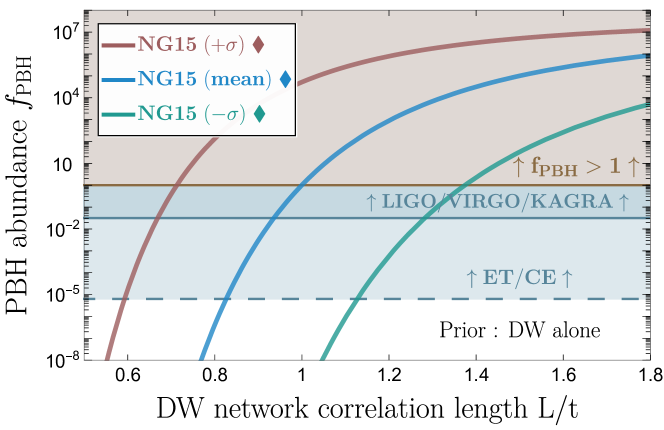
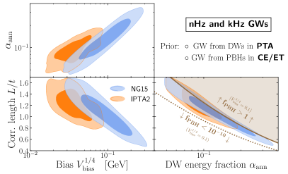
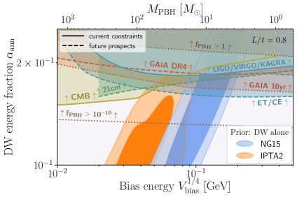
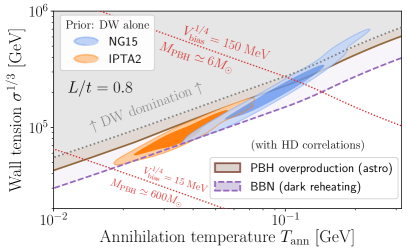
Nano-Hz and kilo-Hz SGWB from DW networks — We have selected five points from the NG15 posterior distribution marked with diamonds in the right panel of Fig. 1. These points include the mean and its $1\sigma$ (68$\%$) confidence interval. For each of those points, we display the PBH abundance as a function of the correlation length $L$ in Fig. 2. The most stringent current constraints on these PBHs stem from the non-detection of a kilo-Hertz SGWB, which would be indicative of PBH binary mergers. They are derived from the ongoing searches by Earth-based interferometers LVK [54, 55, 56, 57, 58]. Looking ahead, the most optimistic forecasts for detection are associated with the next generation of Earth-based interferometers Einstein Telescope and the Cosmic Explorer (ET/CE) [81, 82], assuming that all the astrophysical foregrounds would be subtracted [51]. In the left panel of Fig. 3, we illustrate the preferred range of DW parameters that simultaneously account for the nano-Hz PTA signal and source kilo-Hz GW within the future detectability range of CE/ET [81, 82]. This scenario becomes feasible as soon as $L/t\gtrsim 0.6$.

Figure 4: Bayesian factors $\mathcal{B}_{Y,X}$, with values significantly above 0 suggest support for interpretation $Y$ over $X$. Conversely, values close to 0 indicate no clear preference between $X$ and $Y$. We evaluate the DW interpretation of the PTA signal in two scenarios: with (dashed) and without (solid) contributions from SMBH binaries, comparing these to the interpretation based solely on SMBH binaries. For the SMBH binaries, we consider two modeling approaches: a power-law with a spectral tilt of $\gamma=13/3$ (blue), and a power-law derived from the simulated $\tt{GWOnly-Ext}$ library, which incorporates astrophysical priors [15] (red). Both models assume circular orbits and binary evolution driven by GWs only, see App. C for the details. DW networks with larger correlation length $L$ produce more PBHs, leading to tighter PBH overclosure bound, which in turn diminishes the quality of the PTA signal fit. The Bayes factor shows a significant decrease for the DW-only interpretation, while the reduction is more moderate in the combined DW+SMBH interpretation. Please see Tab. 1 for the Bayes factors across various scenarios, and Fig. 7 for the same figure with IPTA2 dataset.

Additional PBH probes — In the right panel of Fig. 3, we show additional detection probes of PBHs that are formed under the hypothesis that the PTA signal arises from a DW network. Firstly, accretion of PBHs leads to X-ray emissions that can modify the ionization fraction after recombination, leading to signatures in CMB [59, 60, 61] and 21 cm line surveys [83, 84, 85]. Secondly, weak lensing effects from PBHs can cause transient shifts in stars positions which could be detected in GAIA data [86, 87, 88]. We fixed the correlation length to $L=0.8t$, keeping in mind that PBH constraints and prospects would become stronger for larger $L$.

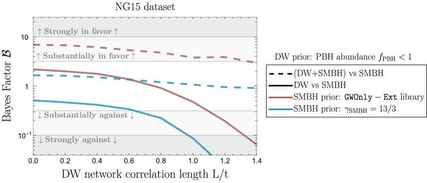
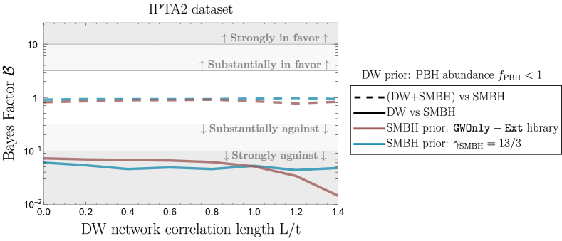
Bayesian analysis — In Fig. 4, we show how Bayes factors $\mathcal{B}_{Y,X}$ evolve as a function of the PBH abundance, which increase as a function of the correlation length $L/t$. The PBH overclosure bound can worsen the quality of both DW and DW+SMBH interpretation of NG15 signal. The impact on IPTA2 is more moderate and reported to appendix. We model the SGWB from SMBH binaries with and without astrophysical priors, see App. C for the details.

V.   CONCLUSION

We have conducted a Bayesian analysis of the NG15 and the IPTA2 datasets, examining the hypothesis that the PTA SGWB signal originates from a long-lived DW networks which annihilated in the early universe, possibly combined with a contribution from SMBH binaries which accounts for astrophysical priors. We have reported new results concerning the modeling of PBH formation during the annihilation of long-lived DW network. The details are referred in the companion paper [51]. We find the DW interpretation of NG15 preferred to the GW-driven SMBH binary interpretation by a Bayes Factor of $\mathcal{B}=6.6$, neglecting for PBH formation. Accounting for PBHs formation, the Bayes factor falls to $\mathcal{B}=0.9$ or lower if the network correlation length is $L\gtrsim 0.8t$. Those PBHs with masses $M_{\rm PBH}=11^{+13}_{-6}M_{\mathSun}$ for NG15 and $M_{\rm PBH}=97^{+88}_{-46}M_{\mathSun}$ for IPTA2 can undergo binary mergers and source kilo-Hz SGWB in the detectability range of future Earth-based interferometers ET/CE as soon as $L/t\gtrsim 0.6$.

This study enhances our comprehension of PBHs formation during the annihilation of long-lived DW networks, addressing gaps in previous literature [49, 52, 53]. It precisely characterizes the subset of DWs that collapse into PBHs – termed late-annihilators – and develop a method to calculate their abundance using percolation theory. Although the DW interpretation of the PTA signal has been explored in numerous studies [96, 48, 97, 34, 15, 98, 99, 89, 35, 100, 101, 102, 103], this work is pioneering in demonstrating that such a scenario can yield a PBH population within the observable range. Furthermore, the Bayesian analysis improve previous works by incorporating uncertainties in the determination of the SGWB peak in lattice simulations [47], and modeling SMBH binaries with and without astrophysical priors.

We conclude that one can range DW networks alongside the two other early-universe GW sources, which can concurrently account for PTA signal and produce multi-solar-mass PBHs. Firstly, there are slowly-completing first-order phase transitions [104, 21], which overproduce PBHs for completion rate smaller than $\beta/H\sim 6$. Secondly, there are scalar-induced GW which overproduce PBHs in the Gaussian limit [23, 105, 106].

Appendix A Bayesian analysis of PTA signal

A.1.   GW-induced pulsar timing residuals

GW are linear tensor perturbations to the flat spacetime metric $g_{ab}=\eta_{ab}+h_{ab}$. In presence of a GW propagating along unit vector $\hat{\Omega}$, the frequency $\nu$ observed at Earth of a pulse emitted by a pulsar $I$ propagating along the unit vector $-\hat{p}$ is shifted according to [107, 108, 109]:

$$\frac{\delta\nu_{I}}{\nu}=-\Lambda^{ab}\left[h_{ab}(t_{e},\vec{x}_{e})-h_{ab}(t_{I},\vec{x}_{I})\right],\qquad\textrm{with}\quad\Lambda^{ab}\equiv\frac{1}{2}\frac{\hat{p}^{a}\hat{p}^{b}}{1+\hat{\Omega}\cdot\hat{p}}.$$ (15)

($\vec{x}_{e}$, $t_{e}$) and ($\vec{x}_{I}$, $t_{I}=t_{e}-D$) are Earth and pulsar coordinates, $D$ being the earth-pulsar distance. The quantity $\Lambda^{ab}$ depends on the angle between the Earth, the pulsar and the GW source. The anomalous residual in arrival time of pulses emitted by a given pulsar is given by the integral of the accumulated frequency shift over time:

$$R_{I}(t)\equiv-\int_{0}^{t}\frac{\delta\nu_{I}}{\nu}dt.$$ (16)

We are searching for stochastic gravitational wave backgrounds (SGWBs). In order to extract this information and disentangle it from pure noise, we introduce the cross-power spectral density of the time residual between two pulsars $I$ and $J$:

$$S_{R,I,J}(f)\equiv\int_{-\infty}^{+\infty}d\tau\,e^{2\pi if\tau}\left<R_{I}(t)R_{J}(t+\tau)\right>.$$ (17)

Plugging Eqs. (15) and (16) into Eq. (17), we obtain:

$$S_{R,IJ}(f)=\frac{\Gamma_{IJ}}{12\pi^{2}}\frac{1}{f^{3}}h_{c}^{2}(f)=\frac{\Gamma_{IJ}}{8\pi^{4}}\frac{H_{0}^{2}}{f^{5}}\Omega_{\rm GW},$$ (18)

where $\Gamma_{IJ}$ are the so-called Helling-Down (HD) cross-correlation coefficients [110]:

$$\Gamma_{IJ}=\frac{\delta_{IJ}}{2}+\frac{1}{2}+3(1-\cos{\theta_{IJ}})\left[\ln{\left(\frac{1-\cos{\theta_{IJ}}}{2}\right)-\frac{1}{6}}\right],$$ (19)

where $\theta_{IJ}$ is the angle difference between of pulsars $I$ and $J$ seen from the Earth. The quantity $h_{c}$ is the characteristic strain of the SGWB. It is defined from its power spectral density $S_{h}(f)$:

$$h_{c}^{2}\equiv fS_{h}(f),\qquad\textrm{with}\quad S_{h}(f)\equiv\int_{-\infty}^{+\infty}d\tau\,e^{2\pi if\tau}\left<h_{ab}(t)h^{ab}(t+\tau)\right>.$$ (20)

The term $\Omega_{\rm GW}$ is the fraction of the universe energy attributed to the SGWB:

$$\Omega_{\rm GW}(f)\equiv\frac{1}{\rho_{c}}\frac{d\rho_{\rm GW}}{d\ln{f}},\qquad\textrm{with}\quad\rho_{\rm GW}=\frac{\left<\dot{h}_{ab}\dot{h}_{ab}\right>}{32\pi G},\quad\textrm{and}\quad\left<\dot{h}_{ab}\dot{h}_{ab}\right>=8\pi^{2}\int_{0}^{\infty}df\,f^{2}S_{h}(f),$$ (21)

where $\rho_{c}=3M_{\rm pl}^{2}H_{0}^{2}$ and $H_{0}$ is today Hubble constant.

Figure 5: LEFT: We compare the $68\%$ and $90\%$ preferred regions, with and without incorporating Helling-Down (HD) inter-pulsar cross-correlations. This means using Eq. (18) with either $\Gamma_{IJ}$ given by Eq. (19), or simply setting $\Gamma_{IJ}=\delta_{IJ}$. The latter approach speeds up MCMC sampling by approximately a factor of 5. RIGHT: We compare the modes “enterprise” and “ceffyl” of ${\tt PTArcade}$. The former performs a MCMC sampling over the complete likelihood, including all noise parameters from each pulsar. The latter performs a MCMC sampling on a reduced likelihood built from the free spectrum template, cf. the violins in Fig. 1-left, speeding up the calculation by approximately a factor $10^{4}$. We use the mode “enterprise” with HD correlations for the remainder of this study.

A.2.   Noise analysis

Likelihood function — The theoretical prediction of pulse arrival times can achieve precision up to $100\leavevmode\nobreak\ \rm ns$ [111, 112, 113] using timing models embedded in software tools such as $\tt TEMPO2$ [114] or $\tt PINT$ [115], both of which are integrated into ${\tt ENTERPRISE}$ [116]. The predicted time residuals can be described by a deterministic part $\vec{R}_{\rm det}$ which can be minimised by the timing model and a stochastic part which contains the SGWB signal along with various sources of noises:

$$\vec{R}_{\rm th}=\vec{R}_{\rm det}+\vec{R}_{\rm GW}+\sum_{n}\vec{R}_{\rm noise}^{(n)},$$ (22)

where vector components denote different times of observation and distinct pulsars. The $n$-sum runs over the different types of noise: red noise, dispersion measure noise, white noise and jitter noise [117, 118, 119]. Each source of noise can be modeled as a Gaussian process with a covariance matrix of Fourier coefficients denoted by $\left[S_{n}\right]$. The likelihood for observing a time series of residuals $\vec{R}_{\rm obs}$ assuming all the model parameters contained in $\vec{R}_{\rm th}$, denoted by $\vec{\theta}$, can be written schematically as [117, 118, 119]

$$\mathcal{P}(\vec{R}_{\rm obs}|\vec{\theta})=\frac{\exp\left[-\frac{1}{2}\vec{R}_{\rm obs}^{T}C^{-1}\vec{R}_{\rm obs}\right]}{\sqrt{(2\pi)\det(C)}},\qquad\textrm{with}\quad{C}=\Delta f\times\vec{\mathcal{F}}\left(\left[S_{R,IJ}\right]+\sum_{n}\left[S_{n}\right]\right)\vec{\mathcal{F}}^{-1}.$$ (23)

The quantity $\left[S_{R,IJ}\right]$ is the covariance matrix of the SGWB signal in Eq. (18) expanded over the $k$ sampling frequencies $f_{k}=k\Delta f$ with $\Delta f=1/T$ the frequency spacing and $T$ the observation time. The quantity $\mathcal{F}$ is a vector of sine and cosine converting objects from Fourier representation to time representation. In order to remain schematic, we have omitted the deterministic component $\vec{R}_{\rm det}$. We refer to [117, 118, 119] for the precise likelihood definition, and [120] for a review of the statistical analysis procedure. The likelihood $\mathcal{P}(\vec{R}_{\rm obs}|\vec{\theta})$ in Eq. (23) can be calculated using the code ${\tt ENTERPRISE}$ [116] and ${\tt enterprise\_extensions}$ [121].

Posterior distribution — Given observed data, the goal of the GW cosmologist or astronomer is to calculate the probability distribution for certain model parameters, e.g the DW network or SMBH binary parameters. This is encoded in the posterior distribution, $\mathcal{P}(\vec{\theta}|\vec{R}_{\rm obs})$, which illustrates the probability distribution of model parameters $\vec{\theta}$ given the observed data $\vec{R}_{\rm obs}$. It is related to the likelihood function via Bayes’s theorem

$$\mathcal{P}(\vec{\theta}|\vec{R}_{\rm obs})=\frac{\mathcal{P}(\vec{R}_{\rm obs}|\vec{\theta})\mathcal{P}(\vec{\theta})}{\mathcal{P}(\vec{R}_{\rm obs})}.$$ (24)

The term $\mathcal{P}(\vec{\theta})$ denotes the prior distribution, which reflects our initial knowledge of the parameters before observing the data. $\mathcal{P}(\vec{R}_{\rm obs})$ represents the marginal likelihood or evidence, serving as a normalizing factor to guarantee that the integration of the posterior distribution equals 1. The posterior distribution $\mathcal{P}(\vec{\theta}|\vec{R}_{\rm mes})$ in Eq. (24) can be reconstituted by sampling over the model parameters $\vec{\theta}$ using a Markov Chain Monte-Carlo (MCMC) code. For this purpose, the code ${\tt enterprise\_extensions}$ [121] embde the parallel-tempering MCMC code ${\tt PTMCMC}$ [122]. Since we are not interested in the posterior dependence on noise parameters, we marginalize over them by integrating Eq. (24) over all of them. This can be trivially accomplished by visualizing only the relevant entries from the MCMC chains.

Figure 6: LEFT: the quantity $\epsilon_{\rm GW}$ determines the amplitude of the SGWB from DW networks, see Eq. (27). Lattice simulations suggest $\epsilon_{{\rm GW}}=0.7\pm 0.4$ [47]. We compare the posteriors with this quantity being fixed to the central value $\epsilon_{\rm GW}=0.7$ or marginalized over the interval $\epsilon_{{\rm GW}}\in[0.3,1.1]$. We adopt the latter choice in the rest of this work. RIGHT: we present the posterior distribution in the plane $T_{\rm ann}-\sigma^{1/3}$ instead of $V_{\rm bias}^{1/4}-\alpha_{\rm ann}$, under the assumption of SM reheating (BBN prior evaded), no PBH prior (omitted), while varying $\epsilon_{\rm GW}$ within its error interval and including HD correlations, like in Fig. 1-right.

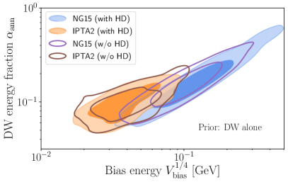
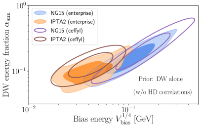
PTArcade — All the steps described beforehand can be realised at once using the wrapper ${\tt PTArcade}$ [69]. We considered the first $14$ frequency bins of NG15 [6] and the first 13 frequency bins of IPTA2 [9]. We used ${\tt GetDist}$ tool [123] to visualize the posteriors. We included $5\times 10^{5}$ steps and discarded 25$\%$ of each MCMC chain as burn-in. We use the mode “enterprise” of ${\tt PTArcade}$, which accounts for the full likelihood in Eq. (23). We included the HD correlation defined in Eq. (19). Each Bayesian analysis takes around $300$ hours per CPU. We estimated that omitting the HD correlation speeds up the calculation by a factor $5$ while the mode “ceffyl” which uses the free spectrum templates from $\tt ceffyl$ [124, 125] allows to calculate posteriors within a few minutes on a single CPU. We compare the posteriors distribution for the different modes in Fig. 5. Despite the time-saving alternatives, all the analyses in this study were conducted using the most precise modes. The violin-shaped posteriors of the PTA signals shown in Fig. 1-left were not computed in this work but were imported directly from NG15 and IPTA2.

A.3.   Bayes factor.

To evaluate how well the observed PTA data $\vec{R}_{\rm obs}$ supports one theoretical model $X$ over another $Y$, we can rely on the Bayesian factor:

$$\mathcal{B}_{Y,X}\equiv\frac{\mathcal{P}(\vec{R}_{\rm obs}|Y)}{\mathcal{P}(\vec{R}_{\rm obs}|X)}.$$ (25)

The software ${\tt enterprise\_extensions}$ [121] can be used to calculate $\mathcal{B}_{Y,X}$ by sampling the two models $X$ and $Y$ at the same time, with a new parameter $m\in\vec{\theta}$ labelling the two models, e.g. $m_{1}$ and $m_{2}$. Then the ratio of likelihoods turns into a ratio of posteriors [120]:

$$\mathcal{B}_{Y,X}=\frac{\mathcal{P}(m_{1}|\vec{R}_{\rm obs})}{\mathcal{P}(m_{2}|\vec{R}_{\rm obs})}.$$ (26)

According to Jeffrey’s scale [126, 127], evidence for or against an interpretation is barely worth mentioning for $|{\log}_{10}{\mathcal{B}_{Y,X}}|<0.5$, becomes substantial for $>0.5$, strong for $>1$, very strong for $>1.5$ and decisive for $>2$.

A.4.   Bayesian analysis conducted in this work.

In this work, we perform various types of Bayesian analysis of PTA datasets, including either SGWB from DW networks, from SMBH binaries or a combination of them, with various priors for both signals: SM or dark reheating, PBH overproduction bound for different values of the correlation length included or not, and astrophysical priors on SMBH binaries included or not. We compare the different models using the Bayes factor in Table 1 and provide the the mean values of the posteriors for model parameters in Table 2. The impact of the PBH abundance on the Bayes factor, through the DW network correlation length, can be appreciated in Figs. 4 and 7.

Figure 7: Similar to Fig. 4, but for the IPTA2 dataset, we analyze the Bayes factor which compares the predictive power of the DW and DW+SMBH interpretations of the PTA signal against the sole SMBH binary interpretation. Two distinct models of the SGWB originating from SMBH binaries are considered, as detailed in App. C. A greater correlation length $L$ implies a higher abundance of PBHs and stricter constraints due to potential PBH overproduction. The influence of PBH abundance on the IPTA2 fit is less pronounced than in the NG15 dataset. We refer to Tab. 1 for values of Bayes factors in different scenarios.

Appendix B DW interpretation

B.1.   SGWB signal.

The GW power spectrum today produced by long-lived DWs annihilating at a temperature $T_{\rm ann}$ can be expressed as [45, 46, 47]:

$$\Omega_{\rm GW}h^{2}=\mathcal{D}\frac{3}{32\pi}\epsilon_{{\rm GW}}\alpha_{\rm ann}^{2}S(f),$$ (27)

where $\mathcal{D}$ is the redshift factor:

$$\mathcal{D}\simeq 3.49\times 10^{-5}\left(\frac{g_{*}(T_{\rm ann})}{10.75}\right)\left(\frac{10.75}{g_{s,*}(T_{\rm ann})}\right)^{4/3}.$$ (28)

The dimensionless factor $\epsilon_{{\rm GW}}$ encodes deviation from the quadrupole formula [40] with lattice simulations suggesting [47]:

$$\epsilon_{{\rm GW}}=0.7\pm 0.4.$$ (29)

We model the spectral function:

$$S(f)=\frac{2}{\left(f/f_{\rm peak}\right)+\left(f_{\rm peak}/f\right)^{3}},$$ (30)

where the IR slope is $\Omega_{\rm GW}\propto f^{3}$ to respect causality [128, 129, 130, 131] and the UV slope is $\Omega_{\rm GW}\propto f^{-1}$ as suggested by lattice simulations results [47] (though more complicated spectra are possible, see e.g. [41]). The peak frequency today is given by

$$f_{\rm peak}=\frac{a(t_{\rm ann})}{a(t_{0})}H(t_{\rm ann})\simeq 1.08\leavevmode\nobreak\ {\rm nHz}\left(\frac{g_{\star}(T_{\rm ann})}{10.75}\right)^{1/2}\times\left(\frac{10.75}{g_{*s}(T_{\rm ann})}\right)^{1/3}\left(\frac{T_{\rm ann}}{10\leavevmode\nobreak\ \rm MeV}\right).$$ (31)

B.2.   Priors

Prior on ${\epsilon}_{{\rm GW}}$ — In order to accounts for the uncertainties in the GW modeling, we consider $\epsilon_{{\rm GW}}$ in Eq. (29) as a model parameter with a prior $\epsilon_{{\rm GW}}\in[0.3,1.1]$, over which we marginalize at the end in all the Bayesian analysis of this work. The impact on the posterior distribution of this choice with respect to fixing $\epsilon_{{\rm GW}}=0.7$ can be appreciated in the left panel of Fig. (6).

BBN prior — The presence of extra number $\Delta N_{\rm eff}$ of relativistic degrees of freedom (DoFs) at BBN and CMB would change the expansion rate of the universe and impact the CMB data or the abundance of light elements [132, 133]. In [51], we show that DW network contribute to the number of relativistic DoFs as:

$$\Delta N_{\rm eff}=\frac{8}{7}\left(\frac{{g_{*}(T_{0})}}{2}\right)\left(\frac{11}{4}\right)^{4/3}\alpha_{\rm DW}(T)\simeq 7.4\,\alpha_{\rm ann}\leavevmode\nobreak\ \lesssim\leavevmode\nobreak\ 0.4,$$ (32)

where $g_{*}(T_{0})\simeq 3.38$. We choose a conservative bound $\Delta N_{\rm eff}\lesssim 0.4$ [134]. Two scenarios must be distinguished according to whether upon annihilating the DW network reheates dark DoFs or Standard Model (SM) DoFs. In the first case, the constraint in Eq. (32) must be applied to all the parameter space. In the second case, the bound Eq. (32) is relaxed if DW annihilate above the neutrino decoupling temperature $T_{\rm ann}\gtrsim 1\leavevmode\nobreak\ \rm MeV$ [135, 136, 137]. We find that only the first scenario is constraining DW interpretation of PTA, see the dashed purple line in Fig. 6-right and Figs. 1-right.

DW-domination prior — Another bounds comes from the possibility for DWs to dominate the energy budget of the universe when $t_{\rm ann}\gtrsim\textrm{Min}(t_{\rm dom},t_{\rm dom}^{\rm unbias})$ according to whether the DW network energy is dominated by its volume or surface contribution. For annihilating DW network, we find that $t_{\rm dom}<t_{\rm dom}^{\rm unbias}$ always hold, hence we have the bound:

$$\alpha_{\rm ann}\leavevmode\nobreak\ \gtrsim\leavevmode\nobreak\ C_{d}^{-1}.$$ (33)

Since it is less constraining that the PBH prior discussed next, we do not include the DW-domination prior in this work. We however indicate this region with a gray dotted line in Fig. 6-right and Figs. 1-right.

PBH prior — One of the novelty of this work is to be able to include PBH overproduction as a prior in the Bayesian analysis. Since the PBH abundance is very sensitive on the model parameter, we considered sufficient to content with the DM overclosure bound:

$$f_{\rm PBH}<1,$$ (34)

with $f_{\rm PBH}$ given in Eq. (13), instead of the more precise astrophysical constraints from LVK and CMB, see main text. The abundance of PBHs is in particular very sensitive to the correlation length $L$, whose precise value remains uncertain (see however below Eq. (1)). Therefore, either we fix it to $L/t=0.8$ or treat it as a free parameter within the range $L/t\in[X,1.5]$, with $X$ varying from $X=0$ to $X=1.4$, see Tab. 1.

Appendix C DW + SMBH interpretation

C.1.   SGWB from SMBH binaries

Single SMBH binary– It is generally accepted that most large galaxies have a supermassive black hole (SMBH) at their center [138]. These galaxies grow over time by merging with others, leading to scenarios where a single galaxy might host several SMBHs. When these SMBHs are sufficiently close, they could potentially form a binary system. The GW power radiated by a circular binary system of masses $m_{1}$ and $m_{2}$ in the quadrupole approximation reads [139]:

$$\frac{dE_{\rm GW}}{dt_{r}}=\frac{32}{5}\frac{c^{5}}{G}\left(\frac{\pi G\mathcal{M}f_{r}}{c^{3}}\right)^{10/3},$$ (35)

where $t_{r}$ and $f_{r}$ are the time and GW frequency measured in the binary rest frame. They are related to the observed GW frequency by $f_{r}=f(1+z)$ where $z$ is the source redshift and to the orbital frequency by $f_{r}=2f_{\rm orb}$. The quantity $\mathcal{M}=(m_{1}m_{2})^{3/5}/(m_{1}+m_{2})^{1/5}$ is the chirp mass. Equating Eq. (35) with the derivative of the orbital energy $E_{\rm orb}=-Gm_{1}m_{2}/2R$ using Kepler’s law $\omega_{\rm orb}^{2}=G(m_{1}+m_{2})/R^{3}$, we obtain the so-called “residence time” per logarithmic frequency interval:

$$\frac{dt_{r}}{d\ln{f_{r}}}=\frac{5}{96\pi^{8/3}}\left(\frac{c^{3}}{G\mathcal{M}}\right)^{5/3}f_{r}^{-8/3}.$$ (36)

Plugging Eq. (36) into Eq. (35), we deduce the source-frame GW energy per logarithmic frequency interval [140, 141]:

$$\frac{dE_{\rm gw}}{d\ln{f_{r}}}=\frac{dt}{\ln{f_{r}}}\frac{dE_{\rm gw}}{dt_{r}}=\frac{\pi^{2/3}}{3G}(G\mathcal{M})^{5/3}f_{r}^{2/3}.$$ (37)

Population of SMBH binaries– We consider a population of SMBH binaries with comoving number density per unit redshift and per unit of chirp mass $d^{2}n/dz/d\mathcal{M}$. The associated radiated energy spectrum $d\rho_{\rm GW}/d\ln f$ is [142]:

$$\frac{d\rho_{\rm GW}}{d\ln f}=\frac{\pi}{4}\frac{c^{2}}{G}f^{2}h_{c}^{2}(f)=\int_{0}^{\infty}dz\int_{0}^{\infty}d\mathcal{M}\frac{d^{2}n}{dzd\mathcal{M}}\frac{1}{(1+z)}\frac{dt}{\ln{f_{r}}}\frac{dE_{\rm gw}}{dt_{r}}\bigg{|}_{f_{r}=f(1+z)}.$$ (38)

where $1/(1+z)$ accounts for the cosmological redshifting of the GW energy. Plugging Eq. (37) into Eq. (38), we obtain the characteristic GW strain:

$$h_{c}^{2}(f)=\frac{4}{3\pi^{1/3}c^{2}}\int_{0}^{\infty}dz\int_{0}^{\infty}d\mathcal{M}\left[\frac{(G\mathcal{M})^{5}}{(1+z)f^{4}}\right]^{1/3}\frac{d^{2}n}{dzd\mathcal{M}}.$$ (39)

From the previous equation, we conclude that the SGWB power spectrum of a population of GW-driven coalescing circular SMBH binaries is a power-law:

$$h_{c}(f)=A_{\rm SMBH}\left(\frac{f}{f_{\rm yr}}\right)^{\alpha},\qquad\alpha=-2/3,\quad f_{\rm yr}=1\leavevmode\nobreak\ \rm yr^{-1}\simeq 31.7\leavevmode\nobreak\ \rm nHz,$$ (40)

with amplitude:

$$A_{\rm SMBH}=5\times 10^{-15}\left(\frac{\mathcal{M}_{0}}{10^{9}\leavevmode\nobreak\ \rm M_{\mathSun}}\right)^{5/3}\left(\frac{n_{0}}{2\times 10^{-3}\leavevmode\nobreak\ \rm Mpc^{-3}}\right)I^{1/2},$$ (41)

where $I$ is a dimensionless quantity:

$$I=\int_{0}^{\infty}\frac{dz}{(1+z)^{1/3}}\int_{0}^{\infty}d\mathcal{M}\left(\frac{\mathcal{M}}{\mathcal{M}_{0}}\right)^{5/3}n_{0}^{-1}\frac{d^{2}n}{dzd\mathcal{M}}.$$ (42)

In terms of the fractional energy density, defined in Eq. (21), it gives

$$\Omega_{\rm GW}(f)=\Omega_{\rm SMBH}\left(\frac{f}{f_{\rm yr}}\right)^{n_{t}},\qquad n_{t}=2(1+\alpha)=-2/3,$$ (43)

and in terms of timing residual power spectrum, defined in Eq. (18), it gives

$$S_{R,IJ}(f)=\Gamma_{IJ}\frac{A_{\rm SMBH}}{12\pi^{2}}f_{\rm yr}^{-3}\left(\frac{f}{f_{\rm yr}}\right)^{-\gamma_{\rm SMBH}},\qquad\gamma_{\rm SMBH}=3-2\alpha=13/3.$$ (44)

Figure 8: We show the favored SGWBs from DWs (dashed) and SMBH binaries (dotted), assuming that the PTA signal is a combination of both. Two different models for the SGWB from SMBH binaries are considered. On the left, we use an analytical approach for GW-driven circular binaries, which predicts a power-law SGWB with a spectral tilt of $n_{t}=2/3$, equivalent to $\gamma_{\rm SMBH}=13/3$ in the timing residual power spectrum as indicated by Eq. (44). On the right, we consider the SGWB produced by the population of GW-driven and circular binaries sampled from astrophysical priors, termed as ${\tt GWOnly-Ext}$ library in [15], and accessible in ${\tt PTArcade}$. The $68\%$ and $90\%$ posterior distributions for these SGWBs are depicted using gray bands. We refer to App. C for the details.

Figure 9: We show the posterior distribution for the combined DW+SMBH interpretation of the PTA signal. We consider two types of powerlaws for the SGWB from SMBH binaries. On top, the SGWB is inferred from the purely analytical description of circular and GW-driven binaries, which fixes the spectral tilt to $\gamma_{\rm SMBH}=13/3$ and leaves the amplitude $A_{\rm SMBH}$ as a free parameter. On bottom, the spectral tilt and amplitude $(\gamma_{\rm SMBH},A_{\rm SMBH})$ are drawn from astrophysical priors, still assuming circular and GW-driven binaries, as in [13]. The presence of DW networks is favored by the NG15 data with the posteriors overlapping substantially with the region overproducing PBHs shown in brown. In contrast the IPTA2 posterior is rather flat in DW parameters, showing no preference for such interpretation. We refer to Figs. 4 and 7 for a visualisation of the Bayes factors and to App. C for more details on the astrophysical priors.

Discretization– The data collected by PTAs is segmented into intervals of length $\Delta f=1/T$, with $T$ the time period of observation. The number of binary systems emitting at each logarithmic frequency bin, which is given by ${dt_{r}/d\ln{f_{r}}}$ in Eq. (36), decreases with frequency. When this number approaches one or less, the continuous and uniform spectrum described in Eq.(38) is accounting for fictitious fractional sources and therefore over-estimate the SWGB signal. The continuous distribution of SMBH, $d^{2}n/dzd\mathcal{M}$, must to be replaced with an integer count of SMBH binaries, $N_{ij}$, sorted into bins of redshift $z$ and chirp mass $\mathcal{M}$, and the integral in Eq. (38) must be replaced by a sum [142, 143, 144, 145, 146]:

$$\int dzd\mathcal{M}\cdots\frac{d^{2}n}{dzd\mathcal{M}}\quad\rightarrow\quad\sum_{ij}\cdots N_{ij}.$$ (45)

C.2.   Priors

In this work we considered two types of modeling for the SGWB from SMBH binaries, labelled “$\gamma_{\rm SMBH}=13/3$” and “${\tt GWOnly-Ext}$”, respectively.

Free amplitude – At first we considered the simple analytical powerlaw in Eq. (44) with the amplitude considered as a free parameter:

$$\gamma_{\rm SMBH}=13/3\quad\textrm{and}\quad\log_{\rm 10}(A_{\rm SMBH})\in[-18,\leavevmode\nobreak\ -14].$$ (46)

Astrophysical prior – Then, we consider the same modeling as in [15] where $A_{\rm SMBH}$ and $\gamma_{\rm SMBH}$ are drawn from a Gaussian distribution with mean and covariance matrix:

$${\tt GWOnly-Ext:}\qquad\bm{\mu}_{\rm SMBH}=\begin{pmatrix}-15.6\\ 4.7\end{pmatrix}\,,\qquad\bm{\sigma}_{\rm SMBH}=10^{-1}\times\begin{pmatrix}2.8&-0.026\\ -0.026&1.2\end{pmatrix}\,.$$ (47)

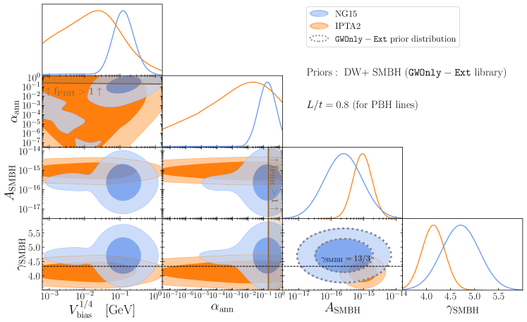
Those values are fitted on the SGWBs calculated from SMBH populations taken from the GWOnly-Ext library [13, 15]. This library only contains circular and GW-driven binaries and use a range of model parameters – like the galaxy stellar mass functions, pair fractions, merger rates, and SMBH-mass versus galaxy-mass relations – that are narrowly defined [15]. The GWOnly-Ext library has been generated using the ${\tt Holodeck}$ program which is still under development [147]. The astrophysical priors on $(\gamma_{\rm SMBH},A_{\rm SMBH})$ in Eq. (47) are accessible in ${\tt PTArcade}$ [69]. The reason why Eq. (47) deviates from the $\gamma_{\rm SMBH}=13/3$ while only considering circular GW-driven binaries can be attributed to the summation in Eq. (45) which reduces the power at higher frequencies [144].

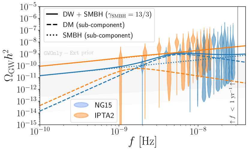
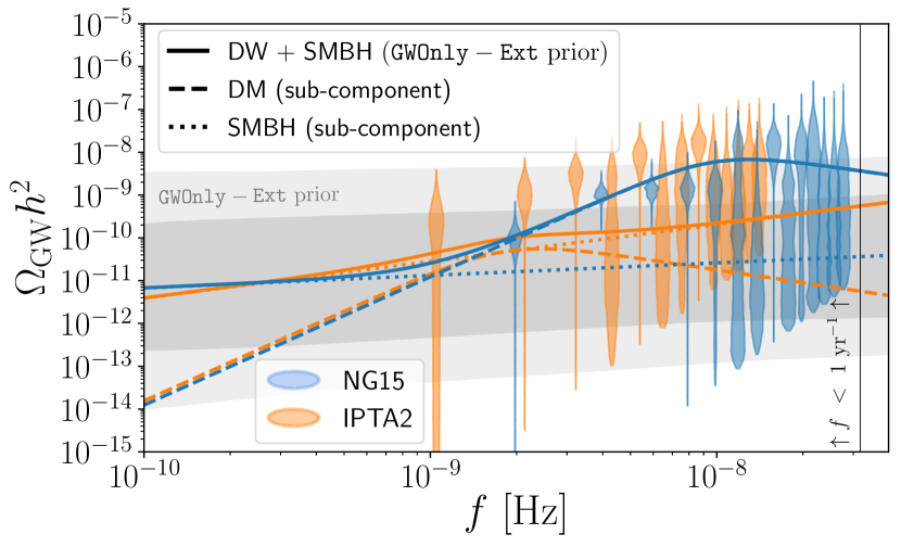
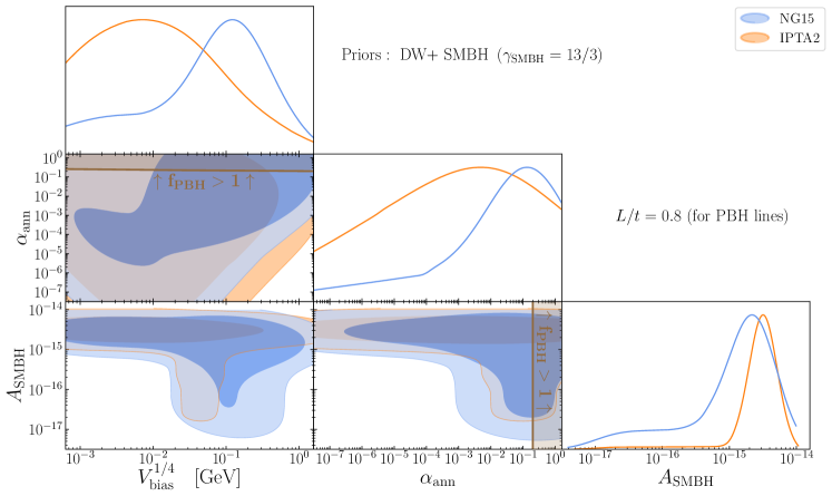
Results – We conduct a Bayesian analysis to interpret the PTA signal as a combination of SGWBs from DW networks and from SMBH binaries, assuming the two different SMBH priors just presented in Eqs. (46) and (47). The preferred SGWBs are depicted in Fig. 8, while the posterior distributions are illustrated in Fig. 9.

Environmental effects – In our study, we have focused exclusively on circular GW-driven binaries. The influence of factors such as binary orbital eccentricity and environmental effects, including binary interaction with nearby stars, accretion disk or third black holes, is generally thought to diminish the power at low frequencies [148, 149, 11, 120]. Consequently, this could cause an increase in $n_{t}$ in Eq. (43) (leading to a redder spectral tilt) and a decrease in $\gamma_{\rm SMBH}$, potentially resembling the contribution from a DW network [15], see Fig. 1-left. Both the DW hypothesis and the SMBH model, accounting for a significant amount of eccentricity and environmental effects, receive comparable support from the PTA data [12, 13, 13, 14]. In the future, extending the observation time and increasing the number of detected pulsars could enable the resolution of individual binary sources [150, 151]. This enhancement would refine the astrophysical priors in Eq. (47) and yield greater precision regarding potential contributions from SGWB originating from primordial sources.

Model X	Model Y	Prior		$\log_{10}{\mathcal{B}_{Y,X}}$
NG15	IPTA2
SMBH ($\gamma_{\rm SMBH}=13/3$)	DW	dark reheating ($\Delta N_{\rm eff}<0.4$)		$-2.62\pm 0.22$	$-2.71\pm 0.20$
		SM reheating		$0.09\pm 0.03$	$-0.98\pm 0.04$
		PBH overproduction ($f_{\rm PBH}<1$)	$L/t\in[0.0,1.5]$	$-0.29\pm 0.03$	$-1.22\pm 0.05$
			$L/t\in[0.2,1.5]$	$-0.33\pm 0.03$	$-1.27\pm 0.05$
			$L/t\in[0.4,1.5]$	$-0.38\pm 0.04$	$-1.34\pm 0.05$
			$L/t\in[0.6,1.5]$	$-0.47\pm 0.04$	$-1.31\pm 0.06$
			$L/t\in[0.8,1.5]$	$-0.65\pm 0.05$	$-1.34\pm 0.07$
			$L/t\in[1.0,1.5]$	$-1.06\pm 0.09$	$-1.28\pm 0.07$
			$L/t\in[1.2,1.5]$	$-1.65\pm 0.20$	$-1.36\pm 0.10$
			$L/t\in[1.4,1.5]$	$-2.87\pm 0.59$	$-1.32\pm 0.15$
	DW+SMBH	dark reheating ($\Delta N_{\rm eff}<0.4$)		$-0.01\pm 0.00$	$0.00\pm 0.01$
		SM reheating		$0.30\pm 0.01$	$-0.09\pm 0.00$
		PBH overproduction ($f_{\rm PBH}<1$)	$L/t\in[0.0,1.5]$	$0.22\pm 0.00$	$-0.04\pm 0.00$
			$L/t\in[0.2,1.5]$	$0.21\pm 0.00$	$-0.03\pm 0.00$
			$L/t\in[0.4,1.5]$	$0.18\pm 0.01$	$-0.03\pm 0.00$
			$L/t\in[0.6,1.5]$	$0.13\pm 0.01$	$-0.03\pm 0.00$
			$L/t\in[0.8,1.5]$	$0.08\pm 0.01$	$-0.03\pm 0.00$
			$L/t\in[1.0,1.5]$	$0.03\pm 0.01$	$-0.02\pm 0.01$
			$L/t\in[1.2,1.5]$	$-0.02\pm 0.01$	$-0.01\pm 0.01$
			$L/t\in[1.4,1.5]$	$-0.07\pm 0.02$	$-0.03\pm 0.01$
SMBH
($\tt{GWOnly-Ext}\textrm{ prior}$)	DW	dark reheating ($\Delta N_{\rm eff}<0.4$)		$-1.69\pm 0.10$	$-2.69\pm 0.25$
		SM reheating		$0.82\pm 0.05$	$-0.94\pm 0.02$
		PBH overproduction ($f_{\rm PBH}<1$)	$L/t\in[0.0,1.5]$	$0.34\pm 0.02$	$-1.14\pm 0.02$
			$L/t\in[0.2,1.5]$	$0.30\pm 0.02$	$-1.16\pm 0.03$
			$L/t\in[0.4,1.5]$	$0.25\pm 0.02$	$-1.17\pm 0.03$
			$L/t\in[0.6,1.5]$	$0.14\pm 0.02$	$-1.18\pm 0.03$
			$L/t\in[0.8,1.5]$	$-0.04\pm 0.02$	$-1.21\pm 0.03$
			$L/t\in[1.0,1.5]$	$-0.32\pm 0.03$	$-1.29\pm 0.04$
			$L/t\in[1.2,1.5]$	$-0.71\pm 0.04$	$-1.47\pm 0.05$
			$L/t\in[1.4,1.5]$	$-1.19\pm 0.09$	$-1.84\pm 0.09$
	DW+SMBH	dark reheating ($\Delta N_{\rm eff}<0.4$)		$-0.08\pm 0.04$	$0.05\pm 0.03$
		SM reheating		$0.98\pm 0.02$	$-0.01\pm 0.01$
		PBH overproduction ($f_{\rm PBH}<1$)	$L/t\in[0.0,1.5]$	$0.84\pm 0.05$	$-0.09\pm 0.02$
			$L/t\in[0.2,1.5]$	$0.83\pm 0.05$	$-0.07\pm 0.02$
			$L/t\in[0.4,1.5]$	$0.79\pm 0.05$	$-0.05\pm 0.02$
			$L/t\in[0.6,1.5]$	$0.73\pm 0.06$	$-0.05\pm 0.02$
			$L/t\in[0.8,1.5]$	$0.68\pm 0.06$	$-0.04\pm 0.02$
			$L/t\in[1.0,1.5]$	$0.58\pm 0.07$	$-0.07\pm 0.03$
			$L/t\in[1.2,1.5]$	$0.59\pm 0.08$	$-0.11\pm 0.03$
			$L/t\in[1.4,1.5]$	$0.47\pm 0.14$	$-0.08\pm 0.05$

Table 1: This table summarizes the Bayesian analysis conducted in this work. The Bayesian factor $\mathcal{B}_{Y,X}$ indicates whether data favors or disfavors interpretation $Y$ with respect to $X$. According to Jeffrey’s criterion [126, 127], evidence is considered barely worth mentioning if $|{\log}_{10}{\mathcal{B}_{Y,X}}|<0.5$, substantial if it is greater than 0.5, strong if it exceeds 1, very strong if it surpasses 1.5, and decisive if it is above 2.

Model	Prior		Parameters $(\log_{10}{X})$	Posterior mean
			NG15	IPTA2
DW	SM reheating		$\alpha_{\rm ann}$	$-0.81\pm 0.18$	$-1.02^{+0.13}_{-0.12}$
			$V_{\rm bias}^{1/4}$	$-0.94^{+0.19}_{-0.17}$	$-1.42\pm 0.14$
			$\sigma^{1/3}$	$5.30\pm 0.16$	$4.94\pm 0.11$
			$T_{\rm ann}$	$-1.04^{+0.15}_{-0.11}$	$-1.45\pm 0.11$
	PBH overproduction
	$L/t\in[0.0,1.5]$	$\alpha_{\rm ann}$	$-0.84^{+0.13}_{-0.16}$	$-0.84^{+0.13}_{-0.16}$
			$V_{\rm bias}^{1/4}$	$-0.96^{+0.15}_{-0.13}$	$-1.49^{+0.19}_{-0.16}$
		$L/t\in[1.0,1.5]$	$\alpha_{\rm ann}$	$-0.97^{+0.10}_{-0.05}$	$-1.10\pm 0.09$
			$V_{\rm bias}^{1/4}$	$-1.07^{+0.14}_{-0.01}$	$-1.46\pm 0.18$
DW+ SMBH	DW: SM reheating $\textrm{SMBH: }\gamma_{\rm SMBH}=13/3$		$\alpha_{\rm ann}$	$-1.4^{+2.4}_{-1.8}$	$-2.0^{+3.2}_{-4.5}$
			$V_{\rm bias}^{1/4}$	$-1.40^{+1.3}_{-0.50}$	$-2.12^{+0.87}_{-0.97}$
			$A_{\rm SMBH}$	$-14.99^{+0.79}_{-0.21}$	$-14.59^{+0.32}_{-0.13}$
			$\gamma_{\rm SMBH}$	$13/3$	$13/3$
	DW: SM reheating $\textrm{SMBH:}\tt{GWOnly-Ext}\textrm{ prior distribution}$		$\alpha_{\rm ann}$	$-0.867^{+0.27}_{-0.090}$	$-2.0^{+3.1}_{-3.7}$
			$V_{\rm bias}^{1/4}$	$-0.99^{+0.27}_{-0.13}$	$-1.98^{+1.1}_{-0.93}$
			$A_{\rm SMBH}$	$-15.62\pm 0.53$	$-15.03\pm 0.26$
			$\gamma_{\rm SMBH}$	$4.71\pm 0.35$	$4.14\pm 0.22$
SMBH	$\gamma_{\rm SMBH}=13/3$		$A_{\rm SMBH}$	$-14.569^{+0.068}_{-0.055}$	$-14.488^{+0.079}_{-0.058}$
	GWOnly-Ext prior distribution		$A_{\rm SMBH}$	$-14.47^{+0.14}_{-0.12}$	$-14.50^{+0.12}_{-0.10}$
			$\gamma_{\rm SMBH}$	$4.08\pm 0.25$	$4.23\pm 0.19$

Table 2: This table displays the mean values of parameters and their $68\%$ confidence intervals. It covers various scenarios: the DW interpretation, the SMBH interpretation, and their combination. Scenario are evaluated with and without PBHs constraints and includes two models of the SGWB from SMBH binaries.

References

- Agazie et al. [2023a] G. Agazie et al. (NANOGrav), The NANOGrav 15-year Data Set: Evidence for a Gravitational-Wave Background, Astrophys. J. Lett. 951, 10.3847/2041-8213/acdac6 (2023a), arXiv:2306.16213 [astro-ph.HE] .
- Antoniadis et al. [2023a] J. Antoniadis et al., The second data release from the European Pulsar Timing Array III. Search for gravitational wave signals, (2023a), arXiv:2306.16214 [astro-ph.HE] .
- Reardon et al. [2023] D. J. Reardon et al., Search for an Isotropic Gravitational-wave Background with the Parkes Pulsar Timing Array, Astrophys. J. Lett. 951, L6 (2023), arXiv:2306.16215 [astro-ph.HE] .
- Xu et al. [2023] H. Xu et al., Searching for the Nano-Hertz Stochastic Gravitational Wave Background with the Chinese Pulsar Timing Array Data Release I, Res. Astron. Astrophys. 23, 075024 (2023), arXiv:2306.16216 [astro-ph.HE] .
- Agazie et al. [2023b] G. Agazie et al. (International Pulsar Timing Array), Comparing recent PTA results on the nanohertz stochastic gravitational wave background, (2023b), arXiv:2309.00693 [astro-ph.HE] .
- Pol et al. [2021] N. S. Pol et al. (NANOGrav), Astrophysics Milestones for Pulsar Timing Array Gravitational-wave Detection, Astrophys. J. Lett. 911, L34 (2021), arXiv:2010.11950 [astro-ph.HE] .
- Chen et al. [2021] S. Chen et al., Common-red-signal analysis with 24-yr high-precision timing of the European Pulsar Timing Array: Inferences in the stochastic gravitational-wave background search 10.1093/mnras/stab2833 (2021), arXiv:2110.13184 [astro-ph.HE] .
- Goncharov et al. [2021] B. Goncharov et al., On the evidence for a common-spectrum process in the search for the nanohertz gravitational-wave background with the Parkes Pulsar Timing Array 10.3847/2041-8213/ac17f4 (2021), arXiv:2107.12112 [astro-ph.HE] .
- Antoniadis et al. [2022] J. Antoniadis et al., The International Pulsar Timing Array second data release: Search for an isotropic gravitational wave background, Mon. Not. Roy. Astron. Soc. 510, 4873 (2022), arXiv:2201.03980 [astro-ph.HE] .
- Sesana et al. [2004] A. Sesana, F. Haardt, P. Madau, and M. Volonteri, Low - frequency gravitational radiation from coalescing massive black hole binaries in hierarchical cosmologies, Astrophys. J. 611, 623 (2004), arXiv:astro-ph/0401543 .
- Burke-Spolaor et al. [2019] S. Burke-Spolaor et al., The Astrophysics of Nanohertz Gravitational Waves, Astron. Astrophys. Rev. 27, 5 (2019), arXiv:1811.08826 [astro-ph.HE] .
- Antoniadis et al. [2023b] J. Antoniadis et al., The second data release from the European Pulsar Timing Array: V. Implications for massive black holes, dark matter and the early Universe, (2023b), arXiv:2306.16227 [astro-ph.CO] .
- Agazie et al. [2023c] G. Agazie et al. (NANOGrav), The NANOGrav 15-year Data Set: Constraints on Supermassive Black Hole Binaries from the Gravitational Wave Background, (2023c), arXiv:2306.16220 [astro-ph.HE] .
- Ellis et al. [2023] J. Ellis, M. Fairbairn, G. Hütsi, J. Raidal, J. Urrutia, V. Vaskonen, and H. Veermäe, Gravitational Waves from SMBH Binaries in Light of the NANOGrav 15-Year Data, (2023), arXiv:2306.17021 [astro-ph.CO] .
- Afzal et al. [2023] A. Afzal et al. (NANOGrav), The NANOGrav 15-year Data Set: Search for Signals from New Physics, Astrophys. J. Lett. 951, 10.3847/2041-8213/acdc91 (2023), arXiv:2306.16219 [astro-ph.HE] .
- Antoniadis et al. [2023c] J. Antoniadis et al. (EPTA), The second data release from the European Pulsar Timing Array: V. Implications for massive black holes, dark matter and the early Universe, (2023c), arXiv:2306.16227 [astro-ph.CO] .
- Caprini et al. [2010] C. Caprini, R. Durrer, and X. Siemens, Detection of gravitational waves from the QCD phase transition with pulsar timing arrays, Phys. Rev. D 82, 063511 (2010), arXiv:1007.1218 [astro-ph.CO] .
- Ratzinger and Schwaller [2021] W. Ratzinger and P. Schwaller, Whispers from the dark side: Confronting light new physics with NANOGrav data, SciPost Phys. 10, 047 (2021), arXiv:2009.11875 [astro-ph.CO] .
- Arzoumanian et al. [2021] Z. Arzoumanian et al. (NANOGrav), Searching for Gravitational Waves from Cosmological Phase Transitions with the NANOGrav 12.5-Year Dataset, Phys. Rev. Lett. 127, 251302 (2021), arXiv:2104.13930 [astro-ph.CO] .
- Bringmann et al. [2023] T. Bringmann, P. F. Depta, T. Konstandin, K. Schmidt-Hoberg, and C. Tasillo, Does NANOGrav observe a dark sector phase transition?, (2023), arXiv:2306.09411 [astro-ph.CO] .
- Gouttenoire [2023] Y. Gouttenoire, First-Order Phase Transition Interpretation of Pulsar Timing Array Signal Is Consistent with Solar-Mass Black Holes, Phys. Rev. Lett. 131, 171404 (2023), arXiv:2307.04239 [hep-ph] .
- Wang et al. [2019] S. Wang, T. Terada, and K. Kohri, Prospective constraints on the primordial black hole abundance from the stochastic gravitational-wave backgrounds produced by coalescing events and curvature perturbations, Phys. Rev. D 99, 103531 (2019), [Erratum: Phys.Rev.D 101, 069901 (2020)], arXiv:1903.05924 [astro-ph.CO] .
- Chen et al. [2020] Z.-C. Chen, C. Yuan, and Q.-G. Huang, Pulsar Timing Array Constraints on Primordial Black Holes with NANOGrav 11-Year Dataset, Phys. Rev. Lett. 124, 251101 (2020), arXiv:1910.12239 [astro-ph.CO] .
- De Luca et al. [2021] V. De Luca, G. Franciolini, and A. Riotto, NANOGrav Data Hints at Primordial Black Holes as Dark Matter, Phys. Rev. Lett. 126, 041303 (2021), arXiv:2009.08268 [astro-ph.CO] .
- Sugiyama et al. [2021] S. Sugiyama, V. Takhistov, E. Vitagliano, A. Kusenko, M. Sasaki, and M. Takada, Testing Stochastic Gravitational Wave Signals from Primordial Black Holes with Optical Telescopes, Phys. Lett. B 814, 136097 (2021), arXiv:2010.02189 [astro-ph.CO] .
- Vaskonen and Veermäe [2021] V. Vaskonen and H. Veermäe, Did NANOGrav see a signal from primordial black hole formation?, Phys. Rev. Lett. 126, 051303 (2021), arXiv:2009.07832 [astro-ph.CO] .
- Kohri and Terada [2021] K. Kohri and T. Terada, Solar-Mass Primordial Black Holes Explain NANOGrav Hint of Gravitational Waves, Phys. Lett. B 813, 136040 (2021), arXiv:2009.11853 [astro-ph.CO] .
- Zhao and Wang [2023] Z.-C. Zhao and S. Wang, Bayesian Implications for the Primordial Black Holes from NANOGrav’s Pulsar-Timing Data Using the Scalar-Induced Gravitational Waves, Universe 9, 157 (2023), arXiv:2211.09450 [astro-ph.CO] .
- Ellis and Lewicki [2021] J. Ellis and M. Lewicki, Cosmic String Interpretation of NANOGrav Pulsar Timing Data, Phys. Rev. Lett. 126, 041304 (2021), arXiv:2009.06555 [astro-ph.CO] .
- Blasi et al. [2021] S. Blasi, V. Brdar, and K. Schmitz, Has NANOGrav found first evidence for cosmic strings?, Phys. Rev. Lett. 126, 041305 (2021), arXiv:2009.06607 [astro-ph.CO] .
- Buchmuller et al. [2020] W. Buchmuller, V. Domcke, and K. Schmitz, From NANOGrav to LIGO with metastable cosmic strings, Phys. Lett. B 811, 135914 (2020), arXiv:2009.10649 [astro-ph.CO] .
- Bian et al. [2021] L. Bian, R.-G. Cai, J. Liu, X.-Y. Yang, and R. Zhou, Evidence for different gravitational-wave sources in the NANOGrav dataset, Phys. Rev. D 103, L081301 (2021), arXiv:2009.13893 [astro-ph.CO] .
- King et al. [2021] S. F. King, S. Pascoli, J. Turner, and Y.-L. Zhou, Gravitational Waves and Proton Decay: Complementary Windows into Grand Unified Theories, Phys. Rev. Lett. 126, 021802 (2021), arXiv:2005.13549 [hep-ph] .
- Madge et al. [2023] E. Madge, E. Morgante, C. P. Ibáñez, N. Ramberg, and S. Schenk, Primordial gravitational waves in the nano-Hertz regime and PTA data – towards solving the GW inverse problem, (2023), arXiv:2306.14856 [hep-ph] .
- Servant and Simakachorn [2023] G. Servant and P. Simakachorn, Constraining Post-Inflationary Axions with Pulsar Timing Arrays, (2023), arXiv:2307.03121 [hep-ph] .
- Depta et al. [2023] P. F. Depta, K. Schmidt-Hoberg, and C. Tasillo, Do pulsar timing arrays observe merging primordial black holes?, (2023), arXiv:2306.17836 [astro-ph.CO] .
- Gouttenoire et al. [2023] Y. Gouttenoire, S. Trifinopoulos, G. Valogiannis, and M. Vanvlasselaer, Scrutinizing the Primordial Black Holes Interpretation of PTA Gravitational Waves and JWST Early Galaxies, (2023), arXiv:2307.01457 [astro-ph.CO] .
- Vilenkin [1981] A. Vilenkin, Gravitational Field of Vacuum Domain Walls and Strings, Phys. Rev. D 23, 852 (1981).
- Preskill et al. [1991] J. Preskill, S. P. Trivedi, F. Wilczek, and M. B. Wise, Cosmology and broken discrete symmetry, Nucl. Phys. B 363, 207 (1991).
- Saikawa [2017] K. Saikawa, A review of gravitational waves from cosmic domain walls, Universe 3, 40 (2017), arXiv:1703.02576 [hep-ph] .
- Gelmini et al. [2021] G. B. Gelmini, S. Pascoli, E. Vitagliano, and Y.-L. Zhou, Gravitational wave signatures from discrete flavor symmetries, JCAP 02, 032, arXiv:2009.01903 [hep-ph] .
- Zeldovich et al. [1974] Y. B. Zeldovich, I. Y. Kobzarev, and L. B. Okun, Cosmological Consequences of the Spontaneous Breakdown of Discrete Symmetry, Zh. Eksp. Teor. Fiz. 67, 3 (1974).
- Vilenkin and Shellard [2000] A. Vilenkin and E. P. S. Shellard, Cosmic Strings and Other Topological Defects (Cambridge University Press, 2000).
- Gleiser and Roberts [1998] M. Gleiser and R. Roberts, Gravitational waves from collapsing vacuum domains, Phys. Rev. Lett. 81, 5497 (1998), arXiv:astro-ph/9807260 .
- Hiramatsu et al. [2010] T. Hiramatsu, M. Kawasaki, and K. Saikawa, Gravitational Waves from Collapsing Domain Walls, JCAP 05, 032, arXiv:1002.1555 [astro-ph.CO] .
- Kawasaki and Saikawa [2011] M. Kawasaki and K. Saikawa, Study of gravitational radiation from cosmic domain walls, JCAP 09, 008, arXiv:1102.5628 [astro-ph.CO] .
- Hiramatsu et al. [2014] T. Hiramatsu, M. Kawasaki, and K. Saikawa, On the estimation of gravitational wave spectrum from cosmic domain walls, JCAP 02, 031, arXiv:1309.5001 [astro-ph.CO] .
- Ferreira et al. [2023] R. Z. Ferreira, A. Notari, O. Pujolas, and F. Rompineve, Gravitational waves from domain walls in Pulsar Timing Array datasets, JCAP 02, 001, arXiv:2204.04228 [astro-ph.CO] .
- Ferrer et al. [2019] F. Ferrer, E. Masso, G. Panico, O. Pujolas, and F. Rompineve, Primordial Black Holes from the QCD axion, Phys. Rev. Lett. 122, 101301 (2019), arXiv:1807.01707 [hep-ph] .
- Ge [2020] S. Ge, Sublunar-Mass Primordial Black Holes from Closed Axion Domain Walls, Phys. Dark Univ. 27, 100440 (2020), arXiv:1905.12182 [hep-ph] .
- Gouttenoire and Vitagliano [2023] Y. Gouttenoire and E. Vitagliano, Primordial Black Holes and Wormholes from Domain Wall Networks, (2023), arXiv:2311.07670 [hep-ph] .
- Gelmini et al. [2023a] G. B. Gelmini, A. Simpson, and E. Vitagliano, Catastrogenesis: DM, GWs, and PBHs from ALP string-wall networks, JCAP 02, 031, arXiv:2207.07126 [hep-ph] .
- Gelmini et al. [2023b] G. B. Gelmini, J. Hyman, A. Simpson, and E. Vitagliano, Primordial black hole dark matter from catastrogenesis with unstable pseudo-Goldstone bosons, (2023b), arXiv:2303.14107 [hep-ph] .
- Nakamura et al. [1997] T. Nakamura, M. Sasaki, T. Tanaka, and K. S. Thorne, Gravitational waves from coalescing black hole MACHO binaries, Astrophys. J. Lett. 487, L139 (1997), arXiv:astro-ph/9708060 .
- Raidal et al. [2019] M. Raidal, C. Spethmann, V. Vaskonen, and H. Veermäe, Formation and Evolution of Primordial Black Hole Binaries in the Early Universe, JCAP 02, 018, arXiv:1812.01930 [astro-ph.CO] .
- Kavanagh et al. [2018] B. J. Kavanagh, D. Gaggero, and G. Bertone, Merger rate of a subdominant population of primordial black holes, Phys. Rev. D 98, 023536 (2018), arXiv:1805.09034 [astro-ph.CO] .
- Abbott et al. [2019] B. P. Abbott et al. (LIGO Scientific, Virgo), Search for Subsolar Mass Ultracompact Binaries in Advanced LIGO’s Second Observing Run, Phys. Rev. Lett. 123, 161102 (2019), arXiv:1904.08976 [astro-ph.CO] .
- De Luca et al. [2020] V. De Luca, G. Franciolini, P. Pani, and A. Riotto, Primordial Black Holes Confront LIGO/Virgo data: Current situation, JCAP 06, 044, arXiv:2005.05641 [astro-ph.CO] .
- Ali-Haïmoud and Kamionkowski [2017] Y. Ali-Haïmoud and M. Kamionkowski, Cosmic microwave background limits on accreting primordial black holes, Phys. Rev. D 95, 043534 (2017), arXiv:1612.05644 [astro-ph.CO] .
- Poulin et al. [2017] V. Poulin, P. D. Serpico, F. Calore, S. Clesse, and K. Kohri, Cmb Bounds on Disk-Accreting Massive Primordial Black Holes, Phys. Rev. D 96, 083524 (2017), arXiv:1707.04206 [astro-ph.CO] .
- Serpico et al. [2020] P. D. Serpico, V. Poulin, D. Inman, and K. Kohri, Cosmic microwave background bounds on primordial black holes including dark matter halo accretion, Phys. Rev. Res. 2, 023204 (2020), arXiv:2002.10771 [astro-ph.CO] .
- Blasi et al. [2023a] S. Blasi, A. Mariotti, A. Rase, A. Sevrin, and K. Turbang, Friction on ALP domain walls and gravitational waves, JCAP 04, 008, arXiv:2210.14246 [hep-ph] .
- Martins et al. [2016] C. J. A. P. Martins, I. Y. Rybak, A. Avgoustidis, and E. P. S. Shellard, Extending the Velocity-Dependent One-Scale Model for Domain Walls, Phys. Rev. D 93, 043534 (2016), arXiv:1602.01322 [hep-ph] .
- Kibble [1976] T. W. B. Kibble, Topology of Cosmic Domains and Strings, J. Phys. A 9, 1387 (1976).
- Sikivie [1982] P. Sikivie, Of Axions, Domain Walls and the Early Universe, Phys. Rev. Lett. 48, 1156 (1982).
- Gelmini et al. [1989] G. B. Gelmini, M. Gleiser, and E. W. Kolb, Cosmology of Biased Discrete Symmetry Breaking, Phys. Rev. D 39, 1558 (1989).
- Kawasaki et al. [2015] M. Kawasaki, K. Saikawa, and T. Sekiguchi, Axion dark matter from topological defects, Phys. Rev. D 91, 065014 (2015), arXiv:1412.0789 [hep-ph] .
- Chang et al. [1999] S. Chang, C. Hagmann, and P. Sikivie, Studies of the motion and decay of axion walls bounded by strings, Phys. Rev. D 59, 023505 (1999), arXiv:hep-ph/9807374 .
- Mitridate et al. [2023] A. Mitridate, D. Wright, R. von Eckardstein, T. Schröder, J. Nay, K. Olum, K. Schmitz, and T. Trickle, PTArcade, (2023), arXiv:2306.16377 [hep-ph] .
- Deng et al. [2017] H. Deng, J. Garriga, and A. Vilenkin, Primordial black hole and wormhole formation by domain walls, JCAP 04, 050, arXiv:1612.03753 [gr-qc] .
- Deng and Vilenkin [2017] H. Deng and A. Vilenkin, Primordial black hole formation by vacuum bubbles, JCAP 12, 044, arXiv:1710.02865 [gr-qc] .
- Deng [2020] H. Deng, Primordial black hole formation by vacuum bubbles. Part II, JCAP 09, 023, arXiv:2006.11907 [astro-ph.CO] .
- Berezin et al. [1983] V. A. Berezin, V. A. Kuzmin, and I. I. Tkachev, THIN WALL VACUUM DOMAINS EVOLUTION, Phys. Lett. B 120, 91 (1983).
- Berezin et al. [1987] V. A. Berezin, V. A. Kuzmin, and I. I. Tkachev, Dynamics of Bubbles in General Relativity, Phys. Rev. D 36, 2919 (1987).
- Blau et al. [1987] S. K. Blau, E. I. Guendelman, and A. H. Guth, The Dynamics of False Vacuum Bubbles, Phys. Rev. D 35, 1747 (1987).
- Maeda [1986] K.-i. Maeda, Bubble dynamics in the expanding universe, Gen. Rel. Grav. 18, 931 (1986).
- Tanahashi and Yoo [2015] N. Tanahashi and C.-M. Yoo, Spherical Domain Wall Collapse in a Dust Universe, Class. Quant. Grav. 32, 155003 (2015), arXiv:1411.7479 [gr-qc] .
- Stauffer [1979] D. Stauffer, Scaling theory of percolation clusters, Phys. Rept. 54, 1 (1979).
- Essam [1980] J. W. Essam, Percolation theory, Reports on Progress in Physics 43, 833 (1980).
- Lalak et al. [1995] Z. Lalak, B. A. Ovrut, and S. Thomas, Large scale structure as a critical phenomenon, Phys. Rev. D 51, 5456 (1995).
- Chen and Huang [2020] Z.-C. Chen and Q.-G. Huang, Distinguishing Primordial Black Holes from Astrophysical Black Holes by Einstein Telescope and Cosmic Explorer, JCAP 08, 039, arXiv:1904.02396 [astro-ph.CO] .
- Pujolas et al. [2021] O. Pujolas, V. Vaskonen, and H. Veermäe, Prospects for probing gravitational waves from primordial black hole binaries, Phys. Rev. D 104, 083521 (2021), arXiv:2107.03379 [astro-ph.CO] .
- Mena et al. [2019] O. Mena, S. Palomares-Ruiz, P. Villanueva-Domingo, and S. J. Witte, Constraining the primordial black hole abundance with 21-cm cosmology, Phys. Rev. D 100, 043540 (2019), arXiv:1906.07735 [astro-ph.CO] .
- Villanueva-Domingo and Ichiki [2021] P. Villanueva-Domingo and K. Ichiki, 21 cm Forest Constraints on Primordial Black Holes 10.1093/pasj/psab119 (2021), arXiv:2104.10695 [astro-ph.CO] .
- Villanueva-Domingo et al. [2021] P. Villanueva-Domingo, O. Mena, and S. Palomares-Ruiz, A brief review on primordial black holes as dark matter, Front. Astron. Space Sci. 8, 87 (2021), arXiv:2103.12087 [astro-ph.CO] .
- Chen et al. [2023] I.-K. Chen, M. Kongsore, and K. Van Tilburg, Detecting Dark Compact Objects in Gaia DR4: A Data Analysis Pipeline for Transient Astrometric Lensing Searches, (2023), arXiv:2301.00822 [astro-ph.GA] .
- Van Tilburg et al. [2018] K. Van Tilburg, A.-M. Taki, and N. Weiner, Halometry from Astrometry, JCAP 07, 041, arXiv:1804.01991 [astro-ph.CO] .
- Verma and Rentala [2022] H. Verma and V. Rentala, Astrometric Microlensing of Primordial Black Holes with Gaia, (2022), arXiv:2208.14460 [astro-ph.GA] .
- Blasi et al. [2023b] S. Blasi, A. Mariotti, A. Rase, and A. Sevrin, Axionic domain walls at Pulsar Timing Arrays: QCD bias and particle friction, (2023b), arXiv:2306.17830 [hep-ph] .
- Coulson et al. [1996] D. Coulson, Z. Lalak, and B. A. Ovrut, Biased domain walls, Phys. Rev. D 53, 4237 (1996).
- Hindmarsh [1996] M. Hindmarsh, Analytic scaling solutions for cosmic domain walls, Phys. Rev. Lett. 77, 4495 (1996), arXiv:hep-ph/9605332 .
- Pujolas and Zahariade [2023] O. Pujolas and G. Zahariade, Domain wall annihilation: A QFT perspective, Phys. Rev. D 107, 123527 (2023), arXiv:2212.11204 [hep-th] .
- Babichev et al. [2022] E. Babichev, D. Gorbunov, S. Ramazanov, and A. Vikman, Gravitational shine of dark domain walls, JCAP 04 (04), 028, arXiv:2112.12608 [hep-ph] .
- Ramazanov et al. [2022] S. Ramazanov, E. Babichev, D. Gorbunov, and A. Vikman, Beyond freeze-in: Dark matter via inverse phase transition and gravitational wave signal, Phys. Rev. D 105, 063530 (2022), arXiv:2104.13722 [hep-ph] .
- Babichev et al. [2023] E. Babichev, D. Gorbunov, S. Ramazanov, R. Samanta, and A. Vikman, NANOGrav spectral index from melting domain walls, (2023), arXiv:2307.04582 [hep-ph] .
- Sakharov et al. [2021] A. S. Sakharov, Y. N. Eroshenko, and S. G. Rubin, Looking at the NANOGrav signal through the anthropic window of axionlike particles, Phys. Rev. D 104, 043005 (2021), arXiv:2104.08750 [hep-ph] .
- Zambujal Ferreira et al. [2022] R. Zambujal Ferreira, A. Notari, O. Pujolàs, and F. Rompineve, High Quality QCD Axion at Gravitational Wave Observatories, Phys. Rev. Lett. 128, 141101 (2022), arXiv:2107.07542 [hep-ph] .
- Bai et al. [2023] Y. Bai, T.-K. Chen, and M. Korwar, QCD-Collapsed Domain Walls: QCD Phase Transition and Gravitational Wave Spectroscopy, (2023), arXiv:2306.17160 [hep-ph] .
- Kitajima et al. [2023] N. Kitajima, J. Lee, K. Murai, F. Takahashi, and W. Yin, Nanohertz Gravitational Waves from Axion Domain Walls Coupled to QCD, (2023), arXiv:2306.17146 [hep-ph] .
- Lu and Chiang [2023] B.-Q. Lu and C.-W. Chiang, Nano-Hertz stochastic gravitational wave background from domain wall annihilation, (2023), arXiv:2307.00746 [hep-ph] .
- Li [2023] X.-F. Li, Probing the high temperature symmetry breaking with gravitational waves from domain walls, (2023), arXiv:2307.03163 [hep-ph] .
- Guo et al. [2023] S.-Y. Guo, M. Khlopov, X. Liu, L. Wu, Y. Wu, and B. Zhu, Footprints of Axion-Like Particle in Pulsar Timing Array Data and JWST Observations, (2023), arXiv:2306.17022 [hep-ph] .
- King et al. [2023] S. F. King, D. Marfatia, and M. H. Rahat, Towards distinguishing Dirac from Majorana neutrino mass with gravitational waves, (2023), arXiv:2306.05389 [hep-ph] .
- Gouttenoire and Volansky [2023] Y. Gouttenoire and T. Volansky, Primordial Black Holes from Supercooled Phase Transitions, (2023), arXiv:2305.04942 [hep-ph] .
- Dandoy et al. [2023] V. Dandoy, V. Domcke, and F. Rompineve, Search for scalar induced gravitational waves in the International Pulsar Timing Array Data Release 2 and NANOgrav 12.5 years dataset, (2023), arXiv:2302.07901 [astro-ph.CO] .
- Franciolini et al. [2023] G. Franciolini, A. Iovino, Junior., V. Vaskonen, and H. Veermae, The recent gravitational wave observation by pulsar timing arrays and primordial black holes: the importance of non-gaussianities, (2023), arXiv:2306.17149 [astro-ph.CO] .
- Allen and Romano [1999] B. Allen and J. D. Romano, Detecting a stochastic background of gravitational radiation: Signal processing strategies and sensitivities, Phys. Rev. D 59, 102001 (1999), arXiv:gr-qc/9710117 .
- Anholm et al. [2009] M. Anholm, S. Ballmer, J. D. E. Creighton, L. R. Price, and X. Siemens, Optimal strategies for gravitational wave stochastic background searches in pulsar timing data, Phys. Rev. D 79, 084030 (2009), arXiv:0809.0701 [gr-qc] .
- Maggiore [2018] M. Maggiore, Gravitational Waves. Vol. 2: Astrophysics and Cosmology (Oxford University Press, 2018).
- Hellings and Downs [1983] R. w. Hellings and G. s. Downs, UPPER LIMITS ON THE ISOTROPIC GRAVITATIONAL RADIATION BACKGROUND FROM PULSAR TIMING ANALYSIS, Astrophys. J. Lett. 265, L39 (1983).
- Hobbs et al. [2006] G. Hobbs, R. Edwards, and R. Manchester, Tempo2, a new pulsar timing package. 1. overview, Mon. Not. Roy. Astron. Soc. 369, 655 (2006), arXiv:astro-ph/0603381 .
- Edwards et al. [2006] R. T. Edwards, G. B. Hobbs, and R. N. Manchester, Tempo2, a new pulsar timing package. 2. The timing model and precision estimates, Mon. Not. Roy. Astron. Soc. 372, 1549 (2006), arXiv:astro-ph/0607664 .
- Hobbs et al. [2009] G. Hobbs, F. Jenet, K. J. Lee, J. P. W. Verbiest, D. Yardley, R. Manchester, A. Lommen, W. Coles, R. Edwards, and C. Shettigara, TEMPO2, a new pulsar timing package. III: Gravitational wave simulation, Mon. Not. Roy. Astron. Soc. 394, 1945 (2009), arXiv:0901.0592 [astro-ph.SR] .
- Hobbs and Edwards [2012] G. Hobbs and R. Edwards, Tempo2: Pulsar Timing Package, Astrophysics Source Code Library, record ascl:1210.015 (2012), ascl:1210.015 .
- Luo et al. [2021] J. Luo et al., PINT: A Modern Software Package for Pulsar Timing, Astrophys. J. 911, 45 (2021), arXiv:2012.00074 [astro-ph.IM] .
- Ellis et al. [2020] J. A. Ellis, M. Vallisneri, S. R. Taylor, and P. T. Baker, Enterprise: Enhanced numerical toolbox enabling a robust pulsar inference suite, Zenodo (2020).
- Arzoumanian et al. [2015] Z. Arzoumanian et al. (NANOGrav), The NANOGrav Nine-year Data Set: Observations, Arrival Time Measurements, and Analysis of 37 Millisecond Pulsars, Astrophys. J. 813, 65 (2015), arXiv:1505.07540 [astro-ph.IM] .
- Arzoumanian et al. [2016] Z. Arzoumanian et al. (NANOGrav), The NANOGrav Nine-year Data Set: Limits on the Isotropic Stochastic Gravitational Wave Background, Astrophys. J. 821, 13 (2016), arXiv:1508.03024 [astro-ph.GA] .
- Agazie et al. [2023d] G. Agazie et al. (NANOGrav), The NANOGrav 15 yr Data Set: Detector Characterization and Noise Budget, Astrophys. J. Lett. 951, L10 (2023d), arXiv:2306.16218 [astro-ph.HE] .
- Taylor [2021] S. R. Taylor, The Nanohertz Gravitational Wave Astronomer, (2021), arXiv:2105.13270 [astro-ph.HE] .
- Taylor et al. [2021] S. R. Taylor, P. T. Baker, J. S. Hazboun, J. Simon, and S. J. Vigeland, enterprise_extensions (2021), v2.3.3.
- Ellis and van Haasteren [2017] J. Ellis and R. van Haasteren, jellis18/ptmcmcsampler: Official release (2017).
- Lewis [2019] A. Lewis, GetDist: a Python package for analysing Monte Carlo samples, (2019), arXiv:1910.13970 [astro-ph.IM] .
- Lamb et al. [2023] W. G. Lamb, S. R. Taylor, and R. van Haasteren, The Need For Speed: Rapid Refitting Techniques for Bayesian Spectral Characterization of the Gravitational Wave Background Using PTAs, (2023), arXiv:2303.15442 [astro-ph.HE] .
- [125] W. G. Lamb and al., https://github.com/astrolamb/ceffyl .
- Jeffreys [1939] H. Jeffreys, Theory of Probability (1939).
- Kass and Raftery [1995] R. E. Kass and A. E. Raftery, Bayes factors, Journal of the american statistical association 90, 773 (1995).
- Durrer and Caprini [2003] R. Durrer and C. Caprini, Primordial Magnetic Fields and Causality, JCAP 11, 010, arXiv:astro-ph/0305059 .
- Caprini et al. [2009] C. Caprini, R. Durrer, T. Konstandin, and G. Servant, General Properties of the Gravitational Wave Spectrum from Phase Transitions, Phys. Rev. D 79, 083519 (2009), arXiv:0901.1661 [astro-ph.CO] .
- Cai et al. [2020] R.-G. Cai, S. Pi, and M. Sasaki, Universal Infrared Scaling of Gravitational Wave Background Spectra, Phys. Rev. D 102, 083528 (2020), arXiv:1909.13728 [astro-ph.CO] .
- Hook et al. [2021] A. Hook, G. Marques-Tavares, and D. Racco, Causal Gravitational Waves as a Probe of Free Streaming Particles and the Expansion of the Universe, JHEP 02, 117, arXiv:2010.03568 [hep-ph] .
- Pitrou et al. [2018] C. Pitrou, A. Coc, J.-P. Uzan, and E. Vangioni, Precision big bang nucleosynthesis with improved Helium-4 predictions, Phys. Rept. 754, 1 (2018), arXiv:1801.08023 [astro-ph.CO] .
- Dvorkin et al. [2022] C. Dvorkin et al., The Physics of Light Relics, in 2022 Snowmass Summer Study (2022) arXiv:2203.07943 [hep-ph] .
- Workman et al. [2022] R. L. Workman et al. (Particle Data Group), Review of Particle Physics, PTEP 2022, 083C01 (2022).
- Bai and Korwar [2022] Y. Bai and M. Korwar, Cosmological constraints on first-order phase transitions, Phys. Rev. D 105, 095015 (2022), arXiv:2109.14765 [hep-ph] .
- Kawasaki et al. [2000] M. Kawasaki, K. Kohri, and N. Sugiyama, MeV scale reheating temperature and thermalization of neutrino background, Phys. Rev. D 62, 023506 (2000), arXiv:astro-ph/0002127 .
- Hasegawa et al. [2019] T. Hasegawa, N. Hiroshima, K. Kohri, R. S. L. Hansen, T. Tram, and S. Hannestad, MeV-scale reheating temperature and thermalization of oscillating neutrinos by radiative and hadronic decays of massive particles, JCAP 12, 012, arXiv:1908.10189 [hep-ph] .
- Kormendy and Ho [2013] J. Kormendy and L. C. Ho, Coevolution (Or Not) of Supermassive Black Holes and Host Galaxies, Ann. Rev. Astron. Astrophys. 51, 511 (2013), arXiv:1304.7762 [astro-ph.CO] .
- Peters and Mathews [1963] P. C. Peters and J. Mathews, Gravitational radiation from point masses in a Keplerian orbit, Phys. Rev. 131, 435 (1963).
- Thorne [1987] K. S. Thorne, GRAVITATIONAL RADIATION, (1987).
- Maggiore [2007] M. Maggiore, Gravitational Waves. Vol. 1: Theory and Experiments (Oxford University Press, 2007).
- Sesana et al. [2008] A. Sesana, A. Vecchio, and C. N. Colacino, The stochastic gravitational-wave background from massive black hole binary systems: implications for observations with Pulsar Timing Arrays, Mon. Not. Roy. Astron. Soc. 390, 192 (2008), arXiv:0804.4476 [astro-ph] .
- McWilliams et al. [2014] S. T. McWilliams, J. P. Ostriker, and F. Pretorius, Gravitational waves and stalled satellites from massive galaxy mergers at , Astrophys. J. 789, 156 (2014), arXiv:1211.5377 [astro-ph.CO] .
- Rosado et al. [2015] P. A. Rosado, A. Sesana, and J. Gair, Expected properties of the first gravitational wave signal detected with pulsar timing arrays, Mon. Not. Roy. Astron. Soc. 451, 2417 (2015), arXiv:1503.04803 [astro-ph.HE] .
- Kelley et al. [2017a] L. Z. Kelley, L. Blecha, L. Hernquist, A. Sesana, and S. R. Taylor, The Gravitational Wave Background from Massive Black Hole Binaries in Illustris: spectral features and time to detection with pulsar timing arrays, Mon. Not. Roy. Astron. Soc. 471, 4508 (2017a), arXiv:1702.02180 [astro-ph.HE] .
- Middleton et al. [2021] H. Middleton, A. Sesana, S. Chen, A. Vecchio, W. Del Pozzo, and P. A. Rosado, Massive black hole binary systems and the NANOGrav 12.5 yr results, Mon. Not. Roy. Astron. Soc. 502, L99 (2021), arXiv:2011.01246 [astro-ph.HE] .
- [147] L. Z. Kelley and al., https://github.com/nanograv/holodeck .
- Sesana [2013] A. Sesana, Insights into the astrophysics of supermassive black hole binaries from pulsar timing observations, Class. Quant. Grav. 30, 224014 (2013), arXiv:1307.2600 [astro-ph.CO] .
- Kelley et al. [2017b] L. Z. Kelley, L. Blecha, and L. Hernquist, Massive Black Hole Binary Mergers in Dynamical Galactic Environments, Mon. Not. Roy. Astron. Soc. 464, 3131 (2017b), arXiv:1606.01900 [astro-ph.HE] .
- Taylor et al. [2020] S. R. Taylor, R. van Haasteren, and A. Sesana, From Bright Binaries To Bumpy Backgrounds: Mapping Realistic Gravitational Wave Skies With Pulsar-Timing Arrays, Phys. Rev. D 102, 084039 (2020), arXiv:2006.04810 [astro-ph.IM] .
- Agazie et al. [2023e] G. Agazie et al. (NANOGrav), The NANOGrav 15 yr Data Set: Search for Anisotropy in the Gravitational-wave Background, Astrophys. J. Lett. 956, L3 (2023e), arXiv:2306.16221 [astro-ph.HE] .