Practical and Asymptotically Exact Conditional Sampling in Diffusion Models

Abstract

Diffusion models have been successful on a range of conditional generation tasks including molecular design and text-to-image generation. However, these achievements have primarily depended on task-specific conditional training or error-prone heuristic approximations. Ideally, a conditional generation method should provide exact samples for a broad range of conditional distributions without requiring task-specific training. To this end, we introduce the Twisted Diffusion Sampler, or TDS. TDS is a sequential Monte Carlo (SMC) algorithm that targets the conditional distributions of diffusion models. The main idea is to use twisting, an SMC technique that enjoys good computational efficiency, to incorporate heuristic approximations without compromising asymptotic exactness. We first find in simulation and on MNIST image inpainting and class-conditional generation tasks that TDS provides a computational statistical trade-off, yielding more accurate approximations with many particles but with empirical improvements over heuristics with as few as two particles. We then turn to motif-scaffolding, a core task in protein design, using a TDS extension to Riemannian diffusion models. On benchmark test cases, TDS allows flexible conditioning criteria and often outperforms the state of the art.

1 Introduction

Conditional sampling is an essential primitive in the machine learning toolkit. One begins with a generative model that parameterizes a distribution $p_{\theta}(x)$ on data $x$, and then augments the model to include information $y$ in a joint distribution $p_{\theta}(x,y)=p_{\theta}(x)p(y~{}|~{}x).$ This joint distribution then implies a conditional distribution $p_{\theta}(x~{}|~{}y),$ from which desired outputs are sampled.

For example, in protein design, $p_{\theta}(x)$ can represent a distribution of physically realizable protein structures, $y$ a substructure that imparts a desired biochemical function, and samples from $p_{\theta}(x~{}|~{}y)$ are then physically realizable structures that contain the substructure of interest [e.g. 29, 32]. In computer vision, $p_{\theta}(x)$ can be a distribution of images, $y$ a class label, and samples from $p_{\theta}(x~{}|~{}y)$ are then images likely to be classified as label $y$ [14].

Diffusion models are a class of generative models that have demonstrated success in conditional generation tasks [15, 23, 28, 32]. They parameterize complicated distributions $p_{\theta}(x)$ through an iterative refinement process that builds up data from noise. When a diffusion model is used for conditional generation, this refinement process is modified to account for conditioning at each step [8, 16, 23, 28].

One approach is conditionally training [e.g. 8, 23], where a diffusion model is trained to incorporate the conditioning information $y$ (either by modifying the model to take $y$ as input or with a classifier that trained alongside the model on partially noised inputs). However, conditional training requires (i) assembling a large set of paired examples of the data and conditioning information $(x,y)$, and (ii) designing and training a task-specific model when adapting to new conditioning tasks. For example, image inpainting and class-conditioned image generation can be both formalized as conditional sampling problems based on the same (unconditional) image distribution $p_{\theta}(x)$; however, the conditional training approach requires training separate models on two curated sets of conditioning inputs.

To help with this expense, a separate line of work uses heuristic approximations that directly operate on unconditional diffusion models: once an unconditional model $p_{\theta}(x)$ is trained, it can be flexibly combined with various conditioning criteria to generate customized outputs. These approaches have been applied to inpainting problems [21, 28, 29], and other general inverse problems [1, 5, 16, 27]. But it is unclear how well these heuristics approximate the exact conditional distributions they are designed to mimic, and on inpainting problems often fail to return outputs consistent with both the conditioning information and unconditional model [35]. These issues are particularly relevant for domains that require accurate conditionals. In molecular design, for example, even a small approximation error could result in atomic structures that have chemically implausible bond distances.

This paper develops a practical and asymptotically exact method for conditional sampling from an unconditional diffusion model. We use sequential Monte Carlo (SMC), a general tool for asymptotically exact inference in sequential probabilistic models [4, 9, 22]. SMC first simulates an ensemble of weighted trajectories, or particles, using a sequence of proposals and weighting mechanisms. It then uses the weighted particles to form an asymptotically exact approximation to a desired target distribution.

The premise of this work is to recognize that the sequential structure of diffusion models permits the application of SMC for sampling from conditional distributions $p_{\theta}(x~{}|~{}y)$. We design an SMC algorithm that leverages twisting, an SMC technique that modifies proposals and weighting schemes to approach the optimal choices [12, 33]. While optimal twisting functions are analytically intractable, we effectively approximate them with recent heuristic approaches to conditional sampling [eg. 16], and then correct the errors by the weighting mechanisms. The resulting algorithm maintains asymptotic exactness to $p_{\theta}(x~{}|~{}y)$ with, and we find empirically that it can improve beyond the heuristics alone with as few as two particles.

We summarize our contributions: (i) We propose a practical SMC algorithm, Twisted Diffusion Sampler or TDS, for asymptotically exact conditional sampling from diffusion models; (ii) We show TDS applies to a range of conditional generation problems, and extends to Riemannian manifold diffusion models; (iii) On MNIST inpainting and class-conditional generation tasks we demonstrate TDS’s empirical improvements beyond heuristic approaches, and (iv) On protein motif-scaffolding problems with short scaffolds TDS provides greater flexibility and achieves higher success rates than the state-of-the-art conditionally trained model.

2 Background: Diffusion models and sequential Monte Carlo

Diffusion models. A diffusion model generates a data point $x^{0}$ by iteratively refining a sequence of noisy data points $x^{t}$, starting from pure noise $x^{T}$. This procedure parameterizes a distribution of $x^{0}$ as the marginal of a length $T$ Markov chain

$$p_{\theta}(x^{0})=\int p(x^{T})\prod_{t=1}^{T}p_{\theta}(x^{t-1}~{}|~{}x^{t})dx^{1:T},$$ (1)

where $p(x^{T})$ is an easy-to-sample noise distribution, and each $p_{\theta}(x^{t-1}~{}|~{}x^{t})$ is the transition distribution defined by the $(T-t)^{\mathrm{th}}$ refinement step.

Diffusion models $p_{\theta}$ are fitted to match a data distribution $q(x^{0})$ from which we have samples. To achieve this goal, a forward process $q(x^{0})\prod_{t=1}^{T}q(x^{t}~{}|~{}x^{t-1})$ is set to gradually add noise to the data, where $q(x^{t}~{}|~{}x^{t-1})=\mathcal{N}\left(x^{t};x^{t-1},\sigma^{2}\right)$, and $\sigma^{2}$ is a positive variance. To fit a diffusion model, one finds $\theta$ such that $p_{\theta}(x^{t-1}~{}|~{}x^{t})\approx q(x^{t-1}~{}|~{}x^{t})$, which is the reverse conditional of the forward process. If this approximation is accomplished for all $t$, and if $T\sigma^{2}$ is big enough that $q(x^{T})$ may be approximated as $q(x^{T})\approx\mathcal{N}(0,T\sigma^{2})=:p(x^{T})$, then we will have $p_{\theta}(x^{0})\approx q(x^{0})$.

In particular, when $\sigma^{2}$ is small enough then the reverse conditionals of $q$ are approximately Gaussian,

$$\begin{split}q(x^{t-1}~{}|~{}x^{t})&\approx\mathcal{N}\left(x^{t-1};x^{t}+\sigma^{2}\nabla_{x^{t}}\log q(x^{t}),\sigma^{2}\right),\end{split}$$ (2)

where $q(x^{t})=\int q(x^{0})q(x^{t}~{}|~{}x^{0})dx^{0}$ and $\nabla_{x^{t}}\log q(x^{t})$ is known as the (Stein) score [28]. To mirror eq. 2, diffusion models parameterize $p_{\theta}(x^{t-1}~{}|~{}x^{t})$ via a score network $s_{\theta}(x^{t},t)$

$$p_{\theta}(x^{t-1}~{}|~{}x^{t}):=\mathcal{N}\left(x^{t-1};x^{t}+\sigma^{2}s_{\theta}(x^{t},t),\sigma^{2}\right).$$ (3)

When $s_{\theta}(x^{t},t)$ is trained to approximate $\nabla_{x^{t}}\log q(x^{t})$, we have $p_{\theta}(x^{t-1}~{}|~{}x^{t})\approx q(x^{t-1}~{}|~{}x^{t})$.

Notably, approximating the score is equivalent to learning a denoising neural network ${\hat{x}}_{\theta}(x^{t},t)$ to approximate $\mathbb{E}_{q}[x^{0}~{}|~{}x^{t}]$. The reason is that by Tweedie’s formula $\nabla_{x^{t}}\log q(x^{t})=(\mathbb{E}_{q}[x^{0}~{}|~{}x^{t}]-x^{t})/t\sigma^{2}$ and one can set $s_{\theta}(x^{t},t):=({\hat{x}}_{\theta}(x^{t},t)-x^{t})/t\sigma^{2}$. The neural network ${\hat{x}}_{\theta}(x^{t},t)$ may be learned by denoising score matching (see [e.g. 15, 30]). For the remainder of paper we drop the argument $t$ in ${\hat{x}}_{\theta}$ and $s_{\theta}$ when it is clear from context.

Sequential Monte Carlo. Sequential Monte Carlo (SMC) is a general tool to approximately sample from a sequence of distributions on variables $x^{0:T}$, terminating at a final target of interest [4, 9, 11, 22]. SMC approximates these targets by generating a collection of $K$ particles $\{x^{t}_{k}\}_{k=1}^{K}$ across $T$ steps of an iterative procedure. The key ingredients are proposals $r_{T}(x^{T})$, $\{r_{t}(x^{t}~{}|~{}x^{t+1})\}_{t=0}^{T-1}$ and weighting functions $w_{T}(x^{T})$, $\{w_{t}(x^{t},x^{t+1})\}_{t=0}^{T-1}$. At the initial step $T$, one draws $x^{T}_{k}\sim r_{T}(x^{T})$ and sets $w^{T}_{k}:=w_{T}(x^{T}_{k})$, and sequentially repeats the following for $t=T-1,\dots,0$:

• resample   $\{x^{t+1:T}_{k}\}_{k=1}^{K}\sim\textrm{Multinomial}(\{x^{t+1:T}_{k}\}_{k=1}^{K};\{w^{t+1}_{k}\}_{k=1}^{K})$

• propose   $x^{t}_{k}\sim r_{t}(x^{t}~{}|~{}x^{t+1}_{k}),\quad k=1,\cdots,K$

• weight    $w^{t}_{k}:=w_{t}(x^{t}_{k},x^{t+1}_{k}),\quad k=1,\cdots,K$

The proposals and weighting functions together define a sequence of intermediate target distributions,

$$\nu_{t}(x^{0:T}):=\frac{1}{\mathcal{L}_{t}}\left[r_{T}(x^{T})\prod_{t^{\prime}=0}^{T-1}r_{t^{\prime}}(x^{t^{\prime}}~{}|~{}x^{t^{\prime}+1})\right]\left[w_{T}(x^{T})\prod_{t^{\prime}=t}^{T-1}w_{t^{\prime}}(x^{t^{\prime}},x^{t^{\prime}+1})\right]$$ (4)

where $\mathcal{L}_{t}$ is a normalization constant.

For example, a classic SMC setting is the state space model [22, Chapter 1] that describes a distribution over a sequence of latent states $x^{0:T}$ and noisy observations $y^{0:T}$. Then each intermediate target $\nu_{t}$ is constructed to be the (potentially intractable) posterior $p(x^{0:T}~{}|~{}y^{t:T})$ given the first $T-t$ observations.

The defining property of SMC is that the weighted particles at each $t$ form discrete approximations $(\sum_{k^{\prime}=1}^{K}w^{t}_{k^{\prime}})^{-1}\sum_{k=1}^{K}w_{t}^{k}\delta_{x^{t}_{k}}(x^{t})$ (where $\delta$ is a Dirac measure) to $\nu_{t}(x^{t})$ that become arbitrarily accurate in the limit that many particles are used [4, Proposition 11.4]. So, by choosing $r_{t}$ and $w_{t}$ so that $\nu_{0}(x^{0})$ matches the desired distribution, one can guarantee arbitrarily low approximation error in the large compute limit.

However, for SMC to be practical with finite compute, the weights must be sufficiently even; if a small fraction of the particles receive weights that are much larger than the rest of the particles the procedure provides a poor approximation of the target.

3 Twisted Diffusion Sampler: SMC sampling for diffusion model conditionals

Consider a conditioning information $y$ associated with a given likelihood function $p_{y|x^{0}}({y}|{x^{0}}).$ We embed $y$ in a joint model over $x^{0:T}$ and $y$ as $p_{\theta}(x^{0:T},y)=p_{\theta}(x^{0:T})p_{y|x^{0}}({y}|{x^{0}}),$ in which $y$ and $x^{1:T}$ are conditionally independent given $x^{0}.$ Our goal is to sample from the conditional distribution $p_{\theta}(x^{0}~{}|~{}y)$ implied by this joint model.

In this section, we develop Twisted Diffusion Sampler (TDS), a practical SMC algorithm targeting $p_{\theta}(x^{0}~{}|~{}y).$ First, we describe how the Markov structure of diffusion models permits a factorization of an extended conditional distribution to which SMC applies. Then, we show how a diffusion model’s denoising predictions support the application of twisting, an SMC technique in which one uses proposals and weighting functions that approximate the “optimal” ones. After introducing a first approximation, we extend TDS to certain “inpainting” problems where $p_{y|x^{0}}({y}|{x^{0}})$ is not smooth, and to Riemannian diffusion models.

// Initial proposal and weight

1 for $k=1:K$ 

2       $x^{T}_{k}\sim p(x^{T})$ $w_{k}\leftarrow\tilde{p}_{k}^{T}=\tilde{p}_{\theta}(y~{}|~{}x^{T})$

3

4for $t=T-1,\cdots,0$ 

       $\{x^{t+1}_{k},\tilde{p}^{t+1}_{k}\}_{k=1}^{K}\sim\mathrm{Multinomial}\left(\{x^{t+1}_{k},\tilde{p}^{t+1}_{k}\}_{k=1}^{K};\{w_{k}\}_{k=1}^{K}\right)$ // resample

5       for $k=1:K$ 

             $\tilde{s}_{k}=({\hat{x}}_{\theta}(x^{t+1}_{k})-x^{t+1}_{k})/t\sigma^{2}+\nabla_{x^{t+1}_{k}}\log\tilde{p}^{t+1}_{k}$ // conditional score approx.

             $x^{t}_{k}\sim\tilde{p}_{\theta}(\cdot{~{}|~{}}x^{t+1}_{k},y):=\mathcal{N}\left(x^{t+1}_{k}+\sigma^{2}\tilde{s}_{k},\tilde{\sigma}^{2}\right)$ // proposal

             $\tilde{p}_{k}^{t}\leftarrow\tilde{p}_{\theta}(y~{}|~{}x^{t})$ // twisting function (in eqs. (11), (18), or (19))

             $w_{k}\leftarrow p_{\theta}(x^{t}_{k}{|}x^{t+1}_{k})\tilde{p}^{t}_{k}/[\tilde{p}_{\theta}(x^{t}_{k}{|}x^{t+1}_{k},y)\tilde{p}^{t+1}_{k}]$ // weight

6            

7      

8      

9

Algorithm 1 Twisted Diffusion Sampler (TDS)

3.1 Conditional diffusion sampling as an SMC procedure

The Markov structure of the diffusion model permits a factorization that is recognizable as the final target of an SMC algorithm. We may write the conditional distribution, extended to additionally include $x^{1:T},$ as

$$p_{\theta}(x^{0:T}~{}|~{}y) =\frac{p_{\theta}(x^{0:T},y)}{p_{\theta}(y)}=\frac{1}{p_{\theta}(y)}\left[p(x^{T})\prod_{t=0}^{T-1}p_{\theta}(x^{t}~{}|~{}x^{t+1})\right]p_{y|x^{0}}({y}|{x^{0}})$$ (5)

with the desired marginal, $p_{\theta}(x^{0}~{}|~{}y).$ Comparing the diffusion conditional of eq. 5 to the SMC target of eq. 4 suggests SMC can be used.

For example, consider a first attempt at an SMC algorithm. Set the proposals as

$$r_{T}(x^{T})=p(x^{T})\quad\mathrm{and}\quad r_{t}(x^{t}~{}|~{}x^{t+1})=p_{\theta}(x^{t}~{}|~{}x^{t+1})\quad\mathrm{for}\quad 1\leq t\leq T,$$ (6)

and weighting functions as

$$w_{T}(x^{T})=w_{t}(x^{t},x^{t+1})=1\quad\mathrm{for}\quad 1\leq t\leq T\quad\mathrm{and}\quad w_{0}(x^{0},x^{1})=p_{y|x^{0}}({y}|{x^{0}}).$$ (7)

Substituting these choices into eq. 4 results in the desired final target $\nu_{0}=p_{\theta}(x^{0:T}~{}|~{}y)$ with normalizing constant $\mathcal{L}_{0}=p_{\theta}(y)$. As a result, the associated SMC algorithm produces a final set of $K$ samples and weights $\{x^{0}_{k};w^{0}_{k}\}_{k=1}^{K}$ that provides an asymptotically accurate approximation $\mathbb{P}_{K}(x^{0}~{}|~{}y):=(\sum_{k}^{K}w^{0}_{k})^{-1}\sum_{k=1}^{K}w^{0}_{k}\delta_{x^{0}_{k}}(x^{0})$ to the desired $p_{\theta}(x^{0}~{}|~{}y).$

The approach above is simply importance sampling with proposal $p_{\theta}(x^{0:T})$; with all intermediate weights set to 1, one can skip resampling steps to reduce the variance of the procedure. Consequently, this approach will be impractical if $p_{\theta}(x^{0}~{}|~{}y)$ is too dissimilar from $p_{\theta}(x^{0})$ as only a small fraction of unconditional samples will have high likelihood: the number of particles required for accurate estimation of $p_{\theta}(x^{0:T}~{}|~{}y)$ is exponential in $\textrm{KL}\left[p_{\theta}(x^{0:T}~{}|~{}y)\;\|\;p_{\theta}(x^{0:T})\right]$ [2].

3.2 Twisted diffusion sampler

Twisting is a technique in SMC literature intended to reduce the number of particles required for good approximation accuracy [12, 13, 22]. Its key idea is to relieve the discrepancy between successive intermediate targets by bringing them closer to the final target. This idea is achieved by introducing a sequence of twisting functions that define new twisted proposals and twisted weighting functions.

Optimal twisting. Consider defining the twisted proposals $r_{t}^{*}$ by multiplying the naive proposals $r_{t}$ described in Section 3.1 by the twisting functions $p_{\theta}(y~{}|~{}x^{t})=\int p_{\theta}(x^{0}~{}|~{}x^{t})p_{y|x^{0}}({y}|{x^{0}})dx^{0}$ as

$$r_{T}^{*}(x^{T}) \propto p(x^{T})p_{\theta}(y{|}x^{T})\ \mathrm{and}\ r_{t}^{*}(x^{t}{|}x^{t+1})\propto p_{\theta}(x^{t}{|}x^{t+1})p_{\theta}(y{|}x^{t})\quad\mathrm{for}\qquad 0\leq t<T.$$ (8)

In fact, $p_{\theta}(y~{}|~{}x^{t})$ are the optimal twisting functions because they permit an SMC sampler that draws exact samples from $p_{\theta}(x^{0:T}~{}|~{}y)$ even when run with a single particle.

To see that even a single particle provides an exact sample, note that by Bayes rule the proposals in eq. 8 reduce to

$$r_{T}^{*}(x^{T}) =p_{\theta}(x^{T}~{}|~{}y)\ \mathrm{and}\ r_{t}^{*}(x^{t}~{}|~{}x^{t+1})=p_{\theta}(x^{t}~{}|~{}x^{t+1},y)\quad\mathrm{for}\qquad 0\leq t<T.$$ (9)

If we choose twisted weighting functions as $w^{*}_{T}(x^{T})=w^{*}_{t}(x^{t},x^{t+1})=1$ for $t=T-1,\dots,0$, then resulting twisted targets $\nu_{t}^{*}$ are all equal to $p_{\theta}(x^{0:T}~{}|~{}y)$. Specifically, substituting $r_{t}^{*}$ and $w_{t}^{*}$ into eq. 4 gives

$$\nu_{t}^{*}(x^{0:T})=\frac{1}{1}\left[p_{\theta}(x^{T}~{}|~{}y)\prod_{t=0}^{T-1}p_{\theta}(x^{t}~{}|~{}x^{t+1},y)\right]\left[1\cdot\prod_{t=0}^{T-1}1\right]=p_{\theta}(x^{0:T}~{}|~{}y),\quad\mathrm{for}\quad 0\leq t\leq T.$$ (10)

However, we cannot readily sample from each $r^{*}_{t}$ because $p_{\theta}(y~{}|~{}x^{t})$ is not analytically tractable. The challenge is that $p_{\theta}(y~{}|~{}x^{t})=\int p_{y|x^{0}}({y}|{x^{0}})p_{\theta}(x^{0}~{}|~{}x^{t})dx^{0}$ depends on $x_{t}$ through $p_{\theta}(x^{0}~{}|~{}x^{t})$. The latter in turn requires marginalizing out $x^{1},\dots,x^{t-1}$ from the joint density $p_{\theta}(x^{0:t-1}~{}|~{}x^{t}),$ whose form depends on $t$ calls to the neural network ${\hat{x}}_{\theta}$.

Tractable twisting. To avoid this intractability, we approximate the optimal twisting functions by

$$\tilde{p}_{\theta}(y~{}|~{}x^{t}):=p_{y|x^{0}}({y}|{{\hat{x}}_{\theta}(x^{t})})\approx p_{\theta}(y~{}|~{}x^{t}),$$ (11)

which is the likelihood function evaluated at ${\hat{x}}_{\theta}(x^{t})$, the denoising estimate of $x^{0}$ at step $t$ from the diffusion model. This tractable twisting function is the key additional ingredient needed to define the Twisted Diffusion Sampler (TDS), (Algorithm 1). We motivate and develop its components below.

The approximation in Equation 11 offers two favorable properties. First, $\tilde{p}_{\theta}(y~{}|~{}x^{t})$ is computable because it depends on $x^{t}$ only though one call to ${\hat{x}}_{\theta},$ instead of an intractable integral over many calls. Second, $\tilde{p}_{\theta}(y~{}|~{}x^{t})$ becomes an increasingly accurate approximation of $p_{\theta}(y~{}|~{}x^{t}),$ as $t$ decreases and $p_{\theta}(x^{0}~{}|~{}x^{t})$ concentrates on $\mathbb{E}_{p_{\theta}}[x^{0}~{}|~{}x^{t}]$, which ${\hat{x}}_{\theta}$ is fit to approximate; at $t=0$, where we can choose ${\hat{x}}_{\theta}(x^{0})=x^{0}$, we obtain $\tilde{p}_{\theta}(y~{}|~{}x^{0})=p_{y|x^{0}}({y}|{x^{0}}).$

We next use eq. 11 to develop a sequence of twisted proposals $\tilde{p}_{\theta}(x^{t}~{}|~{}x^{t+1},y),$ to approximate the optimal proposals $p_{\theta}(x^{t}~{}|~{}x^{t+1},y)$ in eq. 9. Specifically, we define twisted proposals as

$$\tilde{p}_{\theta}(x^{t}~{}|~{}x^{t+1},y) :=\mathcal{N}\left(x^{t};x^{t+1}+\sigma^{2}s_{\theta}(x^{t+1},y);\tilde{\sigma}^{2}\right),$$ (12)

$$\mathrm{where}\quad s_{\theta}(x^{t+1},y) :=s_{\theta}(x^{t+1})+\nabla_{x^{t+1}}\log\tilde{p}_{\theta}(y~{}|~{}x^{t+1})$$ (13)

is an approximation of the conditional score, $s_{\theta}(x^{t+1},y)\approx\nabla_{x^{t+1}}\log p_{\theta}(x^{t+1}~{}|~{}y)$ and $\tilde{\sigma}^{2}$ is the variance of the proposal. For simplicity one could choose each $\tilde{\sigma}^{2}=\sigma^{2}$ to match the variance of the unconditional model $p_{\theta}(x^{t}~{}|~{}x^{t+1})$.

The gradient in eq. 13 is computed by back-propagating through the denoising network ${\hat{x}}_{\theta}(x^{t}).$ Equation 12 builds on previous works (e.g. [26]) that seek to approximate the reversal of a conditional forward noising process. And the idea to backpropagate through the denoising network follows from earlier reconstruction guidance approaches [16, 27] (see related works discussion in Section 4).

To see why $\tilde{p}_{\theta}(x^{t}~{}|~{}x^{t+1},y)$ provides a reasonable approximation of $p_{\theta}(x^{t}~{}|~{}x^{t+1},y)$, notice that if $s_{\theta}(x^{t+1},y)=\nabla_{x^{t+1}}\log q(x^{t+1}~{}|~{}y),$ $\tilde{\sigma}^{2}=\sigma^{2},$ $p_{\theta}=q,$ and $\tilde{p}_{\theta}(y~{}|~{}x^{t})=p_{\theta}(y~{}|~{}x^{t}),$ then

$$\tilde{p}_{\theta}(x^{t}~{}|~{}x^{t+1},y) =\mathcal{N}\left(x^{t};x^{t+1}+\sigma^{2}\nabla_{x^{t+1}}\log q(x^{t+1}~{}|~{}y),\sigma^{2}\right)$$ (14)

$$=q(x^{t}~{}|~{}x^{t+1},y)=p_{\theta}(x^{t}~{}|~{}x^{t+1},y).$$ (15)

In practice, however, we cannot expect to have $\tilde{p}_{\theta}(x^{t}~{}|~{}x^{t+1},y)=p_{\theta}(x^{t}~{}|~{}x^{t+1},y).$ So we must introduce non-trivial weighting functions to ensure the resulting SMC sampler converges to the desired final target. In particular, we define twisted weighting functions as

$$w_{t}(x^{t},x^{t+1}):=\frac{p_{\theta}(x^{t}~{}|~{}x^{t+1})\tilde{p}_{\theta}(y~{}|~{}x^{t})}{\tilde{p}_{\theta}(y~{}|~{}x^{t+1})\tilde{p}_{\theta}(x^{t}~{}|~{}x^{t+1},y)},\qquad t=0,\dots,T-1$$ (16)

and $w_{T}(x^{T}):=\tilde{p}_{\theta}(x^{T})$. The weighting functions in eq. 16 again recover the optimal, constant weighting functions if all other approximations at play are exact.

These tractable twisted proposals and weighting functions define intermediate targets that gradually approach the final target $\nu_{0}=p_{\theta}(x^{0:T}~{}|~{}y)$. Substituting into eq. 4 each $\tilde{p}_{\theta}(x^{t}~{}|~{}x^{t+1},y)$ in eq. 12 for $r_{t}(x^{t}~{}|~{}x^{t+1})$ and $w_{t}(x^{t},x^{t+1})$ in eq. 16 and then simplifying we obtain the intermediate targets

$$\nu_{t}(x^{0:T}) \propto p_{\theta}(x^{0:T}~{}|~{}y)\left[\frac{\tilde{p}_{\theta}(y~{}|~{}x^{t})}{p_{\theta}(y~{}|~{}x^{t})}\prod_{t^{\prime}=0}^{t-1}\frac{\tilde{p}_{\theta}(x^{t^{\prime}}~{}|~{}x^{t^{\prime}+1},y)}{p_{\theta}(x^{t^{\prime}}~{}|~{}x^{t^{\prime}+1},y)}\right].$$ (17)

The right-hand bracketed term in eq. 17 can be understood as the discrepancy of $\nu_{t}$ from the final target $\nu_{0}$ accumulated from step $t$ to $0$ (see Section A.1 for a derivation). As $t$ approaches $0,$ $\tilde{p}_{\theta}(y~{}|~{}x^{t})$ improves as an approximation of $p_{\theta}(y~{}|~{}x^{t}),$ and the $t$-term product inside the bracket consists of fewer terms. Finally, at $t=0,$ because $\tilde{p}_{\theta}(y~{}|~{}x^{0})=p_{\theta}(y~{}|~{}x^{0})$ by construction, eq. 17 reduces to $\nu_{0}(x^{0:T})=p_{\theta}(x^{0:T}~{}|~{}y),$ as desired.

The TDS algorithm and asymptotic exactness. Together, the twisted proposals $\tilde{p}_{\theta}(x^{t}~{}|~{}x^{t+1},y)$ and weighting functions $w_{t}(x^{t},x^{t+1})$ lead to Twisted Diffusion Sampler, or TDS (Algorithm 1). While Algorithm 1 states multinomial resampling for simplicity, in practice other resampling strategies (e.g. systematic [4, Ch. 9]) may be used as well. Under additional conditions, TDS provides arbitrarily accurate estimates of $p_{\theta}(x^{0}~{}|~{}y)$. Crucially, this guarantee does not rely on assumptions on the accuracy of the approximations used to derive the twisted proposals and weights.

Theorem 1.

(Informal) Let $\mathbb{P}_{K}(x^{0})=(\sum_{k^{\prime}}^{K}w_{k^{\prime}})^{-1}\sum_{k=1}^{K}w_{k}\delta_{x_{k}^{0}}(x^{0})$ denote the discrete measure defined by the particles and weights returned by Algorithm 1 with $K$ particles. Under regularity conditions on the twisted proposals and weighting functions, $\mathbb{P}_{K}(x^{0})$ converges setwise to $p_{\theta}(x^{0}~{}|~{}y)$ as $K$ approaches infinity.

Appendix A provides the formal statement with complete conditions and proof.

3.3 TDS for inpainting, additional degrees of freedom

The twisting functions $\tilde{p}_{\theta}(y~{}|~{}x^{t}):=p_{y|x^{0}}({y}|{{\hat{x}}_{\theta}(x^{t})})$ are one convenient option, but are sensible only when $p_{y|x^{0}}({y}|{{\hat{x}}_{\theta}(x^{t})})$ is differentiable and strictly positive. We now show how alternative twisting functions lead to proposals and weighting functions that address inpainting problems and more flexible conditioning specifications. In these extensions, Algorithm 1 still applies with the new definitions of twisting functions. Appendix A provides additional details, including the adaptation of TDS to variance preserving diffusion models [28].

Inpainting. Consider the case that $x^{0}$ can be segmented into observed dimensions $\mathbf{M}$ and unobserved dimensions $\mathbf{\bar{M}}$ such that we may write $x^{0}=[x^{0}_{\mathbf{M}},x^{0}_{\mathbf{\bar{M}}}]$ and let $y=x^{0}_{\mathbf{M}},$ and take $p_{y|x^{0}}({y}|{x^{0}})=\delta_{y}(x^{0}_{\mathbf{M}}).$ The goal, then, is to sample $p_{\theta}(x^{0}~{}|~{}x^{0}_{\mathbf{M}}=y)=p_{\theta}(x^{0}_{\mathbf{\bar{M}}}~{}|~{}x^{0}_{\mathbf{M}})\delta_{y}(x^{0}_{\mathbf{M}}).$ Here we define the twisting function for each $t>0$ as

$$\tilde{p}_{\theta}(y~{}|~{}x^{t},\mathbf{M}):=\mathcal{N}\left(y;{\hat{x}}_{\theta}(x^{t})_{\mathbf{M}},t\sigma^{2}\right),$$ (18)

and set twisted proposals and weights according to eqs. 12 and 16. The variance in eq. 18 is chosen as $t\sigma^{2}=\mathrm{Var}_{p_{\theta}}[x^{t}~{}|~{}x^{0}]$ for simplicity; in general, choosing this variance to more closely match $\mathrm{Var}_{p_{\theta}}[y~{}|~{}x^{t}]$ may be preferable. For $t=0,$ we define the twisting function analogously with small positive variance, for example as $\tilde{p}_{\theta}(y~{}|~{}x^{0})=\mathcal{N}(y;x^{0}_{\mathbf{M}},\sigma^{2}).$ This choice of simplicity changes the final target slightly; alternatively, the final twisting function, proposal, and weights may be chosen to maintain asymptotic exactness (see Section A.2).

Inpainting with degrees of freedom. We next consider the case when we wish to condition on some observed dimensions, but have additional degrees of freedom. For example in the context of motif-scaffolding in protein design, we may wish to condition on a functional motif $y$ appearing anywhere in a protein structure, rather than having a pre-specified set of indices $\mathbf{M}$ in mind. To handle this situation, we (i) let $\mathcal{M}$ be a set of possible observed dimensions, (ii) express our ambivalence in which dimensions are observed as $y$ using randomness by placing a uniform prior on $p(\mathbf{M})=1/|\mathcal{M}|$ for each $\mathbf{M}\in\mathcal{M},$ and (iii) again embed this new variable into our joint model to define the degrees of freedom likelihood by $p(y~{}|~{}x^{0})=\sum_{\mathbf{M}\in\mathcal{M}}p_{\theta}(\mathbf{M},y~{}|~{}x^{0})=|\mathcal{M}|^{-1}\sum_{\mathbf{M}\in\mathcal{M}}p(y~{}|~{}x^{0},\mathbf{M}).$ Accordingly, we approximate $p_{\theta}(y~{}|~{}x^{t})$ with the twisting function

$$\tilde{p}_{\theta}(y~{}|~{}x^{t}):=|\mathcal{M}|^{-1}\sum_{\mathbf{M}\in\mathcal{M}}\tilde{p}_{\theta}(y~{}|~{}x^{t},\mathbf{M}),$$ (19)

with each $\tilde{p}_{\theta}(y~{}|~{}x^{t},\mathbf{M})$ defined as in eq. 18. Notably, Equation 19 and Equation 18 coincide when $|\mathcal{M}|=1.$

The summation in Equation 19 may be computed efficiently because each term in the sum depends on $x^{t}$ only through the same denoising estimate ${\hat{x}}_{\theta}(x^{t},t).$ As a result, the expensive step of computing ${\hat{x}}_{\theta}(x^{t},t)$ can be computed once and the overall run-time is not significantly impacted by using even very large $|\mathcal{M}|$.

3.4 TDS on Riemannian manifolds

TDS extends to diffusion models on Riemannian manifolds with little modification. Riemannian diffusion models [7] are set up similarly as in the Euclidean case, but with conditionals defined using tangent normal distributions parameterized with a score approximation followed by a projection step back to the manifold (see e.g. [3, 7]). When we assume that (as, e.g., in [34]) the model is associated with a denoising network ${\hat{x}}_{\theta}$, twisting functions are also constructed analogously. For conditional tasks defined by positive likelihoods, $\tilde{p}_{\theta}(y~{}|~{}x^{t})$ in eq. 11 applies. For inpainting (and by extension, degrees of freedom), we propose

$$\tilde{p}_{\theta}(y~{}|~{}x^{t})=\mathcal{TN}_{{\hat{x}}_{\theta}(x^{t})_{\mathbf{M}}}(y;0,t\sigma^{2}),$$ (20)

where $\mathcal{TN}_{{\hat{x}}_{\theta}(x^{t})_{\mathbf{M}}}(0,t\sigma^{2})$ is a tangent normal distribution centered on ${\hat{x}}_{\theta}^{\mathbf{M}}(x^{t}).$ As in the Euclidean case, $\tilde{p}_{\theta}(x^{t}~{}|~{}x^{t+1},y)$ is defined with conditional score approximation $s_{\theta}(x^{t+1},y)=s_{\theta}(x^{t+1})+\nabla_{x^{t+1}}\log\tilde{p}(y~{}|~{}x^{t+1})$, which is also computable by automatic differentiation. Appendix B provides details.

4 Related work

There has been much recent work on conditional generation using diffusion models. But these prior works demand either task specific conditional training, or involve unqualified approximations and can suffer from poor performance in practice.

Approaches involving training with conditioning information. There are a variety of works that involve training a neural network on conditioning information to achieve approximate conditional sampling. These works include (i) conditional training with embeddings of conditioning information, e.g. for denoising or deblurring lower resolution images [25], and text-to-image generation [23]), (ii) conditioning training with a subset of the state space, e.g. for protein design [32], and image inpainting [24], (iii) classifier-guidance [8, 28], an approach for generating samples from a diffusion model that fall into a desired class (this strategy requires training a time-dependent classifier to approximate, for each $t,\ p(y~{}|~{}x^{t})$, and training such a time-dependent classifier may be inconvenient and costly), and (iv) classifier-free guidance [14], an approach that builds on the idea of classifier-guidance but does not require training a separate classifier; instead, this technique trains a diffusion model that takes class information as additional input. These conditionally-trained models have the limitation that they do not apply to new types of conditioning information without additional training.

Reconstruction guidance. Outside of the context of SMC and the twisting technique, the use of denoising estimate ${\hat{x}}_{\theta}(x^{t},t)$ to form an approximation $\tilde{p}_{\theta}(x^{t}~{}|~{}x^{t+1},y)$ to $p_{\theta}(x^{t}~{}|~{}x^{t+1},y)$ is called reconstruction guidance [5, 16, 27]. This technique involves sampling one trajectory from $\tilde{p}_{\theta}(x^{t}~{}|~{}x^{t+1},y)$ from $T-1$ to 1, starting with $x^{T}\sim p(x^{T})$. Notably, while this approximation is reasonable, there is no formal guarantee or evaluation criteria on how accurate the approximations, as well as the final conditional samples $x^{0}$, are. Also this approach has empirically been shown to have unreliable performance in image inpainting problems [35].

Replacement method. The replacement method [28] is the most widely used approach for approximate conditional sampling in an unconditionally trained diffusion model. In the inpainting problem, it replaces the observed dimensions of intermediate samples $x^{t}_{\mathbf{M}}$, with a noisy version of observation $x^{0}_{\mathbf{M}}$. However, it is a heuristic approximation and can lead to inconsistency between inpainted region and observed region [20]. Additionally, the replacement method is applicable only to inpainting problems. While recent work has extended the replacement method to linear inverse problems [e.g. 19], the heuristic approximation aspect persists, and it is unclear how to further extend to problems with smooth likelihoods.

SMC-Diff. Most closely related to the present work is SMC-Diff [29], which uses SMC to provide asymptotically accurate conditional samples for the inpainting problem. However, this prior work (i) is limited to the inpainting case, and (ii) provides asymptotically accurate conditional samples only under the assumption that the learned diffusion model exactly matches the forward noising process at every step. Notably, the assumption in (ii) will not be satisfied in practice. Also, SMC-Diff does not leverage the idea of twisting functions.

Langevin and Metropolis-Hastings steps. Some prior work has explored using Markov chain Monte Carlo steps in sampling schemes to better approximate conditional distributions. For example unadjusted Langevin dynamics [28, 16] or Hamiltonian Monte Carlo [10] in principle permit asymptotically exact sampling in the limit of many steps. However these strategies are only guaranteed to target the conditional distributions of the joint model under the (unrealistic) assumption that the unconditional model exactly matches th forward process, and in practice adding such steps can worsen the resulting samples, presumably as a result of this approximation error [18]. By contrast, TDS does not require the assumption that the learned diffusion model exactly matches the forward noising process.

5 Simulation study and conditional image generation

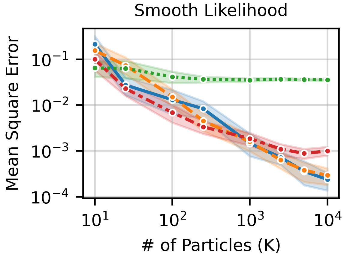
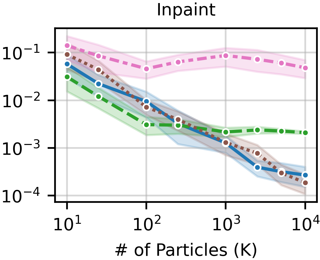
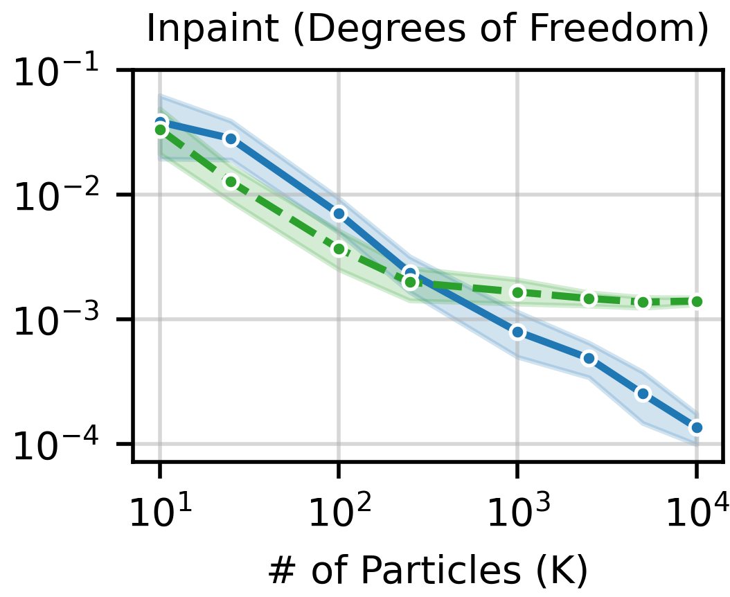
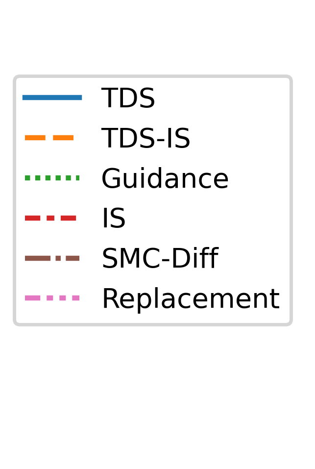
Figure 1: Errors of conditional mean estimations with 2 SEM error bars averaged over 25 replicates. TDS applies to all three tasks and provides increasing accuracy with more particles.

We first test the dependence of the accuracy of TDS on the number of particles in synthetic settings with tractable exact conditionals in Section 5.1. Section 5.2 compares TDS to alternative approaches on MNIST class-conditional generation and inpainting experiment in Appendix C. Additional details for all are included in Appendix C.

Our evaluation includes:

1. TDS: twisted diffusion sampler;

2. TDS-IS: an importance sampler that uses twisted proposals and weight set to $\tilde{p}_{\theta}(y~{}|~{}x^{0})$. TDS-IS can be viewed as TDS without resampling steps;

3. Guidance: viewed as TDS with one particle. This approach coincides with the reconstruction guidance [e.g. 5, 16, 27];

4. IS: the naive importance sampler described in Section 3;

5. Replacement: a heuristic sampler for inpainting tasks that replaces $x^{t}_{\mathbf{M}}$ with a noisy version of the observed $x^{0}_{\mathbf{M}}$ at each $t$ [28];

6. SMC-Diff: an SMC algorithm with replacement method as proposals for inpainting tasks [29]. TDS and SMC-Diff are implemented with sytematic resampling.

Each SMC sampler considered (namely TDS, TDS-IS, IS, and SMC-Diff) forms a discrete approximation to $p_{\theta}(x^{0}~{}|~{}y)$ with $K$ weighted particles $(\sum_{k^{\prime}=1}^{K}w_{k^{\prime}})^{-1}\cdot\sum_{k=1}^{K}w_{k}\delta_{x^{0}_{k}}$. Guidance and replacement methods are considered to form a similar particle-based approximation with $K$ independently drawn samples viewed as $K$ particles with uniform weights.

5.1 Applicability and precision of TDS in two dimensional simulations

We explore two questions in this section: (i) what sorts of conditioning information can be handled by TDS and by other methods, and (ii) how does the precision of TDS depend on the number of particles?

To study these questions, we first consider an unconditional diffusion model $p_{\theta}(x^{0})$ approximation of a bivariate Gaussian. For this choice, the marginals of the forward process are also Gaussian, and so we may define $p_{\theta}(x^{0:T})$ with an analytically tractable score function, rather than approximating it with a neural network. Consequently, we can analyze the performance without the influence of score network approximation errors. And the choice of a two-dimensional diffusion permits very close approximation of exact conditional distributions by numerical integration that can then be used as ground truth.

We consider three test cases defining the conditional information:

1. Smooth likelihood: $y$ is an observation of the Euclidean norm of $x$ with Laplace noise, with $p_{\theta}(y~{}|~{}x^{0})=\exp\{|\|x^{0}\|_{2}-y|\}/2.$ This likelihood is smooth almost everywhere.

2. Inpainting: $y$ is an observation of the first dimension of $x^{0}$, with $p_{\theta}(y~{}|~{}x^{0},\mathbf{M}=0)=\delta_{y}(x^{0}_{0}).$

3. Inpainting with degrees-of-freedom: $y$ is a an observation of either the first or second dimension of $x^{0},$ with $\mathcal{M}=\{0,1\}$ and $p_{\theta}(y~{}|~{}x^{0})=\frac{1}{2}[\delta_{y}(x^{0}_{0})+\delta_{y}(x^{0}_{1})].$

In all cases we fix $y=0$ and consider estimating $\mathbb{E}[x^{0}~{}|~{}y].$

Figure 1 reports the estimation error for the mean of the desired conditional distribution, i.e. $\|\sum w_{k}x^{0}_{k}-\mathbb{E}_{q}[x^{0}~{}|~{}y]\|_{2}$. TDS provides a computational-statistical trade-off: using more particles decreases mean square estimation error at the $O(1/K)$ parametric rate (note the slopes of $-1$ in log-log scale) as expected from standard SMC theory [4, Ch. 11]. This convergence rate is shared by TDS, TDS-IS, and IS in the smooth likelihood case, and shared by TDS, SMCDiff and in the inpainting case; TDS-IS, IS and SMCDiff are applicable however only in these respective cases, whereas TDS applicable in all cases. The only other method which applies to all three settings is Guidance, which in all cases exhibits significant estimation error and does not improve with many particles.

5.2 MNIST class-conditional generation

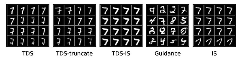
(a) Approximate conditional samples of each method with 64 particles given class $y=7$.

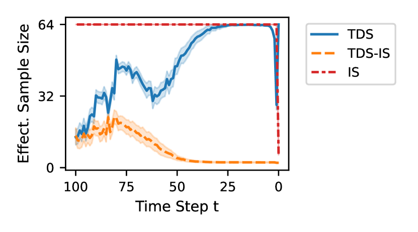
(b) ESS trace avg. over 100 runs ($K=64$)

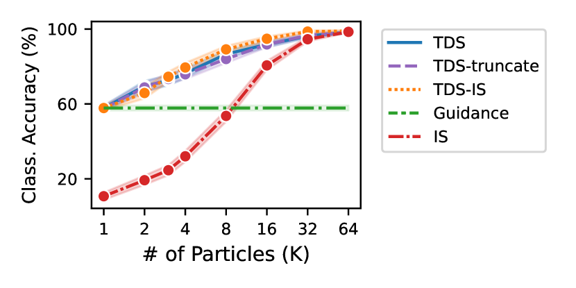
(c) Classification accuracy avg. over 1k runs.

Figure 2: MNIST class-conditional generation. TDS generates a diverse set of desired digits, and has higher particle efficiency compared to other SMC samplers. Notably, TDS with $K=2$ particles outperform the Guidance baseline in terms of classification accuracy.

We next study the performance of TDS on diffusion models with neural network approximations to the score functions. In particular, we study the class-conditional generation task on the MNIST dataset, which involves sampling an image of the digit from $p_{\theta}(x^{0}~{}|~{}y)\propto p_{\theta}(x^{0})p_{y|x^{0}}({y}|{x^{0}})$, where $y$ is a given class of the digit, and $p_{y|x^{0}}({y}|{\cdot})$ denotes the classification likelihood. We compare TDS to TDS-IS, Guidance, and IS, all with $T=100$ sampling steps. In all experiments, we follow the standard practice of returning the denoising mean on the final sample [15]. In addition we include a variation called TDS-truncate that truncates the TDS procedure at $t=10$ and returns ${\hat{x}}_{\theta}(x^{10})$.

To assess the faithfulness of generation, we evaluate classification accuracy on predictions of conditional samples $x^{0}$ given $y$, made by the same classifier that specifies the likelihood. Another metric used for comparing between SMC samplers (namely TDS, TDS-IS and IS) is effective sample size (ESS) , which is defined as $(\sum_{k=1}^{K}w^{t}_{k})^{2}/(\sum_{k=1}^{K}(w^{t}_{k})^{2})$ for $K$ weighted particles $\{x^{t}_{k},w^{t}_{k}\}_{k=1}^{K}$. Note that ESS is always bounded between 0 and $K$.

The results are summarized in Figure 2. To compare generation quality and diversity, we visualize conditional samples given class $y=7$ in Figure 2(a). Samples from Guidance have noticeable artifacts, and most of them do not resemble the digit 7, whereas the other 4 methods produce authentic and correct digits. However, most samples from IS or TDS-IS are identical. By contrast, samples from TDS and TDS-truncate have greater diversity, with the latter exhibiting slightly more variations.

The ESS trace comparison in Figure 2(b) shows that TDS has a general upward trend of ESS approaching $K=64$. Though in the final few steps ESS of TDS drops by a half, it is still higher than that of TDS-IS and IS that deteriorates to around 1 and 6 respectively.

Finally, Figure 2(c) depicts the classification accuracy of all methods against # particles $K$. For all SMC samplers, more particles improve the accuracy, with $K=64$ leading to nearly perfect accuracy. Given the same $K$, TDS and its variants have similar accuracy that outperforms others. This observation suggests that one can use TDS-truncate to avoid effective sample size drop and encourage the generation diversity, without compromising the performance.

TDS can be extended by exponentiating twisting functions with a twist scale. This extension is related to existing literature of classifier guidance [eg. 8] that exponentiates the classification likelihood. We conduct an ablation study on twist scales, and find that moderately large twist scales enhance TDS’s performance especially for small $K$. See Appendix C for details.

6 Case study in computational protein design: the motif-scaffolding problem

We next apply TDS to the motif-scaffolding problem. Section 6.1 introduces the problem. Section 6.2 designs the twisting functions. Section 6.3 examines sensitivity to key hyperparameters. Section 6.4 presents an evaluation on a benchmark set.

6.1 The motif-scaffolding problem and evaluation set-up

The biochemical functions of proteins are typically imparted by a small number of atoms, known as a motif, that are stabilized by the overall protein structure, known as the scaffold [31]. A central task in protein design is to identify stabilizing scaffolds in response to motifs known or theorized to confer biochemical function. Provided with a generative model supported on physically realizable protein structures $p_{\theta}(x^{0})$, suitable scaffolds may be constructed by solving a conditional generative modeling problem [29]. Complete structures are viewed as segmented into a motif $x^{0}_{\mathbf{M}}$ and scaffold $x^{0}_{\mathbf{\bar{M}}},$ i.e. $x^{0}=[x^{0}_{\mathbf{M}},x^{0}_{\mathbf{\bar{M}}}].$ Putative compatible scaffolds are then identified by (approximately) sampling from $p_{\theta}(x^{0}_{\mathbf{\bar{M}}}~{}|~{}x^{0}_{\mathbf{M}}).$

While the conditional generative modeling approach to motif-scaffolding has produced functional, experimentally validated structures for certain motifs [32], the general problem remains open. For example, on a recently proposed benchmark set of motif-scaffolding problems, the state-of-the-art method RFdiffusion, a conditionally trained diffusion model, provides <50% in silico success rates on a majority of test cases [32]. Moreover, current methods for motif-scaffolding require a practitioner to specify the location $\mathbf{M}$ of the motif within the primary sequence of the full scaffold; the choice of $\mathbf{M}$ can require expert knowledge and trial and error.

Evaluation: We use self-consistency evaluation approach for generated backbones [29] that (i) uses fixed backbone sequence design (inverse folding) to generate a putative amino acid sequence to encode the backbone, (ii) forward folds sequences to obtain backbone structure predictions, and (iii) judges the quality of initial backbones by their agreement (or self-consistency) with predicted structures. We inherit the specifics of our evaluation and success criteria set-up following [32], including using ProteinMPNN [6] for step (i) and AlphaFold [17] on a single sequence (no multiple sequence alignment) for (ii).

We hypothesized that improved motif-scaffolding could be achieved through accurate conditional sampling. To this end, we applied TDS to FrameDiff, a Riemannian diffusion model that parameterizes protein backbones as a collection of $N$ rigid bodies (known as residues) in the manifold $SE(3)^{N}$ [34]. Each of the $N$ elements of $SE(3)$ consists of a $3\times 3$ rotation matrix and a $3$ dimensional translation that parameterize the locations of the three backbone atoms of each residue N, C$\alpha$ and C through a rigid body transformation of a residue centered at the origin with idealized bond-lengths and angles.

6.2 Likelihood and twisting functions with degrees of freedom

The basis of our approach to the motif scaffolding problem is analogous to the inpainting case described in Section 3.3. We let $p_{y|x^{0}}({y}|{x^{0}})=\delta_{y}(x^{0}_{\mathbf{M}}),$ where $y\in SE(3)^{M}$ describes the coordinates of backbone atoms of an $M<N$ residue motif, and $\mathbf{M}\subset\{1,\dots,N\}$ with $|\mathbf{M}|=M$ denotes the indices of residues in the backbone chain corresponding to the motif.

To define a twisting function, we use a tangent normal approximation to $p_{\theta}(y~{}|~{}x^{t})$ as introduced in eq. 20. In this case the tangent normal factorizes across each residue and across the rotational and translational components. The translational components are represented in $\mathbb{R}^{3},$ and so are treated as in the previous Euclidean cases, using the variance preserving extension described in Appendix A. For the rotational components, represented in the special orthogonal group $SO(3),$ the tangent normal may be computed as described in Appendix B, using the known exponential map on $SO(3)$. In particular, we use as the twisting function

$$\tilde{p}_{\theta}(y~{}|~{}x^{t},\mathbf{M})=\prod_{m=1}^{|\mathbf{M}|}\mathcal{N}(y^{T}_{m};{\hat{x}}_{\theta}(x^{t})^{T}_{\mathbf{M}_{m}},1-\bar{\alpha}_{t})\mathcal{TN}_{{\hat{x}}_{\theta}(x^{t})^{R}_{\mathbf{M}_{m}}}(y_{m}^{R};0,\bar{\sigma}_{t}^{2}),$$ (21)

where $y^{T}_{m},{\hat{x}}_{\theta}(x^{t})^{T}_{\mathbf{M}_{m}}\in\mathbb{R}^{3}$ represent the translations associated with the $m^{th}$ residue of the motif and its prediction from $x^{t},$ and $y^{R}_{m},{\hat{x}}_{\theta}(x^{t})^{R}_{\mathbf{M}_{m}}\in SO(3)$ represent the analogous quantities for the rotational component. Next, $1-\bar{\alpha}_{t}=\mathrm{Var}[x^{t}~{}|~{}x^{t}]$ and $\bar{\sigma}_{t}^{2}$ is the time of the Brownian motion associated with the forward process at step $t$ [34]. For further simplicity, our implementation further approximates log density of the tangent normal on rotations using the squared Frobenius norm of the difference between the rotations associated with the motif and the denoising prediction (as in [32]), which becomes exact in the limit that $\bar{\sigma}_{t}$ approaches 0 but avoids computation of the inverse exponential map and its Jacobian.

Motif location degrees of freedom. We next address the requirement that motif location indices within the scaffold be specified in advance by incorporating it as a degree of freedom. Specifically, we (i) treat the sequence indices as a mask $\mathbf{M},$ (ii) let $\mathcal{M}$ be the set of all possible masks of size equal to the length of the motif, and (iii) apply Equation 19 to average over possible motif placements. However the number of motif placements grows combinatorially with number of residues in the backbone and motif and so allowing for every possible motif placement is in general intractable. So we (i) restrict to masks which place the motif indices in a pre-specified order that we do not permute and do not separate residues that appear contiguously in source PDB file, and (ii) when there are still too many possible placements sub-sample randomly to obtain the set of masks $\mathcal{M}$ of at most some maximum size (# Motif Locs.). We do not enforce the spacing between segments specified in the “contig” description described by [32].

Motif rotation and translation degrees of freedom. We similarly seek to eliminate the rotation and translation of the motif as a degree of freedom. We again represent our ambivalence about the rotation of the motif with randomness, augment our joint model to include the rotation with a uniform prior, and write

$$p_{y|x^{0}}({y}|{x^{0}})=\int p(R)p_{y|x^{0}}({y}|{x^{0},R})\quad\mathrm{for}\quad p_{y|x^{0}}({y}|{x^{0},R})=\delta_{Ry}(x^{0})$$ (22)

and with $p(R)$ the uniform density (Haar measure) on SO(3), and $Ry$ represents rotating the rigid bodies described by $y$ by $R.$ For computational tractability, we approximate this integral with a Monte Carlo approximation defined by subsampling a finite number of rotations, $\mathcal{R}=\{R_{k}\}$ (with $|\mathcal{R}|=$# Motif Rots. in total). Altogether we have

$$\tilde{p}_{\theta}(y~{}|~{}x^{t})=|\mathcal{R}|^{-1}\cdot|\mathcal{M}|^{-1}\sum_{R\in\mathcal{R}}\sum_{\mathbf{M}\in\mathcal{M}}\tilde{p}_{\theta}(Ry~{}|~{}x^{t},\mathbf{M}).$$

The subsampling above introduces the number of motif locations and rotations subsampled as a hyperparameter. Notably the conditional training approach does not immediately address these degrees of freedom, and so prior work randomly sampled a single value for these variables [29, 31, 32].

6.3 Sensitivity to number of particles, degrees of freedom and twist scale

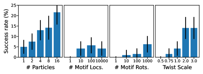
Figure 3: Dependence of TDS motif-scaffolding success rate (test case 5IUS) on (Left) number of particles, (Middle Left) number of motif location degrees of freedom, (Middle Right) number of rotation degrees of freedom, and twist scale. Using more particles and allowing more degrees of freedom increases success rates.

We first explore the impact of different hyper-parameters on a single problem in the benchmark (5IUS); we first studied a single problem to reduce computational burden, before addressing the full benchmark set. Figure 3 compares the impact of several TDS hyperparameters on success rates for a single motif (5IUS) from the benchmark set [32]. We found success rate to increase monotonically with the number of particles used, with $K=16$ providing a roughly $4$ fold increase in empirical success rate (Figure 3 Left). Non-zero success rates in this setting with FrameDiff required accounting for motif locations (Figure 3 Left uses $1{,}000$ possible motif locations and $100$ possible rotations). The success rate was 0% without accounting for these degrees of freedom, and increased with larger numbers of locations and rotations (Figure 3 Middle-Left and Middle-Right).

We also explored including a heuristic twist scale as considered for class-conditional generation in Section 5.2; in this case, the twist scale is a multiplicative factor on the logarithm of the twisting function. Larger twist scales gave higher success rates on 5IUS (Figure 3 Right), though we found this trend was not monotonic for all problems (see Figure K in Appendix D). We use an effective sample size threshold of $K/2$ in all cases, that is, we trigger resampling steps only when the effective sample size falls below this level.

6.4 TDS on motif-scaffolding benchmark set

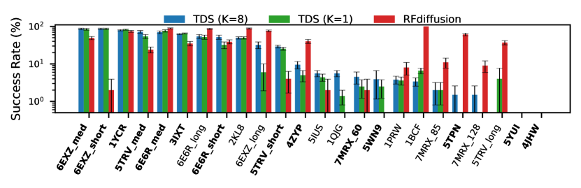
Figure 4: Results on full motif-scaffolding benchmark set. The y-axis is the fraction of successes across at least $200$ replicates. Error bars are $\pm 2$ standard errors of the mean. Problems with scaffolds shorter than 100 residues are bolded. TDS (K=8) outperforms the state-of-the-art (RFdiffusion) on most problems with short scaffolds.

We evaluated TDS on a benchmark set of 24 motif-scaffolding problems and compare to the previous state of the art, RFdiffusion. We ran TDS with K=1 and K=8 particles, twist scale=2, and $100$ rotations and $1{,}000$ motif location degrees of freedom ($100{,}000$ combinations total). As described in Section 3.3, this inclusion incurs minimal additional computational expense.

Figure 4 presents success rates for each problem. TDS with 8 particles provides higher empirical success than TDS with 1 particle (guidance) on most benchmark problems, including two cases (5TPN and 7MRX_128) with zero success rate, and two problems (6EXZ_long and 1QJG) on which the empirical success rate increased by at least 4-fold. The improvement is more pronounced on “hard” problems; TDS with 8 particles outperforms TDS with 1 particle in 11/13 cases where both approaches have success rates between 0% and 75%. We found variable sample efficiency (quantified by ESS) in different settings (see Appendix D). We next compare performance to RFdiffusion. RFdiffusion operates on the same rigid body representation of protein backbones as FrameDiff, but is conditionally trained for the motif-scaffolding task. TDS provides higher success rates on half (11/22) of the problems on which either TDS and RFdiffusion have non-zero success rates. This performance is obtained despite the fact that FrameDiff, unlike RFdiffusion, is not trained to perform motif scaffolding.

The division between problems on which each method performs well is primarily explained by total scaffold length, with TDS providing higher success rates on smaller scaffolds. Of the 22 problem with non-zero success rates, TDS has higher success on 9/12 problems with scaffolds shorter than 100 residues and 2/10 problems with 100 residue or longer scaffolds; the successes in this latter group (5UIS and 1QJG) both have discontiguous motif segments, on which the motif-placement degrees of freedom may be particularly helpful. We suspect the performance gap between TDS and RFdiffusion on longer scaffolds owes to (i) the underlying model; long backbones generated unconditionally by RFdiffusion are designable (backbone scRMSD<2Å) with significantly higher frequency than those generated by FrameDiff [34] and (ii) that unlike RFdiffusion, FrameDiff can not condition on the fixed motif sequence.

7 Discussion

We propose TDS, a practical and asymptotically exact conditional sampling algorithm for diffusion models. We compare TDS to other approaches that do not require conditional training. We demonstrate the effectiveness and flexibility of TDS on MNIST class conditional generation and inpainting tasks. On protein motif-scaffolding problems with short scaffolds, TDS outperforms the current (conditionally trained) state of the art.

A limitation of TDS is its requirement for additional computational resources to simulate multiple particles. While in some cases we see improved performance with as few as two particles, how many particles is enough is problem dependent. Furthermore, the computational efficiency depends on how closely the twisting functions approximate exact conditionals, which depends on both the unconditional model and the conditioning information. Moreover, choosing twisting functions for generic, nonlinear, constraints may be challenging. Addressing these limitations and improving the computational efficiency of the TDS is an important direction for future work.

Appendix

[appendixtoc] [appendixtoc]l1

Appendix A Twisted Diffusion Sampler additional details

TDS algorithm for variance exploding diffusion models.

TDS as developed in Section 3 is based on a “variance exploding” (VE) diffusion model [28] with the variance schedule set to use a constant variance $\sigma^{2}$ at each timestep. Here we describe the general setting with non-constant variance schedules. VE diffusion models define the forward process $q$ by

$$q(x^{1:T}~{}|~{}x^{0}):=\prod_{t=1}^{T}q(x^{t}~{}|~{}x^{t-1}),\qquad q(x^{t}~{}|~{}x^{t-1}):=\mathcal{N}(x^{t};x^{t-1},\sigma_{t}^{2}).$$ (23)

where $\sigma_{t}^{2}$ is an increasing sequence of variances such that $q(x^{T})\approx\mathcal{N}(0,\bar{\sigma}_{T}^{2})$, with $\bar{\sigma}_{t}^{2}:=\sum_{t^{\prime}=1}^{t}\sigma_{t^{\prime}}^{2}$ for $t=1,\cdots,T$. And so one can set $p(x^{T})=\mathcal{N}(0,\bar{\sigma}_{T}^{2})$ to match $q(x^{T})$. Notably, Equation 23 implies the conditional $q(x^{t}~{}|~{}x^{0})=\mathcal{N}(x^{t};x^{0},\bar{\sigma}_{t}^{2})$.

The reverse diffusion process $p_{\theta}$ is parameterized as

$$p_{\theta}(x^{0:T}):=p(x^{T})\prod_{t=T}^{1}p_{\theta}(x^{t-1}~{}|~{}x^{t}),\qquad p_{\theta}(x^{t-1}~{}|~{}x^{t}):=\mathcal{N}(x^{t-1};x^{t}+\sigma_{t}^{2}s_{\theta}(x^{t},t),\sigma_{t}^{2})$$ (24)

where the score network $s_{\theta}$ is modeled through a denoiser network ${\hat{x}}_{\theta}$ by $s_{\theta}(x^{t},t):=({\hat{x}}_{\theta}(x^{t},t;\theta)-x^{t})/\bar{\sigma}_{t}^{2}$. Note that the constant schedule is a special case where $\sigma_{t}^{2}=\sigma^{2}$, and $\bar{\sigma}_{t}^{2}=t\sigma^{2}$ for all $t$.

The TDS algorithm for general VE models is described in Algorithm 1, where $t\sigma^{2}$ in Algorithm 1 is replaced by $\bar{\sigma}^{2}$ and $\sigma^{2}$ in Algorithm 1 is replaced by $\sigma_{t}^{2}$.

Extension to variance preserving diffusion models.

Another widely used diffusion framework is variance preserving (VP) diffusion models [15]. VP models define the forward process $q$ by

$$q(x^{1:T}~{}|~{}x^{0}):=\prod_{t=1}^{T}q(x^{t}~{}|~{}x^{t-1}),\qquad q(x^{t}~{}|~{}x^{t-1}):=\mathcal{N}(x^{t};\sqrt{1-\sigma_{t}^{2}}x^{t-1},\sigma_{t}^{2})$$ (25)

where $\sigma_{t}^{2}$ is a sequence of increasing variances chosen such that $q(x^{T})\approx\mathcal{N}(0,1)$, and so one can set $p(x^{T})=\mathcal{N}(0,1)$. Define $\alpha_{t}:=1-\sigma_{t}^{2}$, $\bar{\alpha}_{t}:=\prod_{t^{\prime}=1}^{t}\alpha_{t^{\prime}}$, and $\bar{\sigma}_{t}^{2}:=1-\bar{\alpha}_{t}$. Then the marginal conditional of eq. 23 is $q(x^{t}~{}|~{}x^{0})=\mathcal{N}(x^{t};\sqrt{\bar{\alpha}_{t}}x^{0},\bar{\sigma}_{t}^{2})$. The reverse diffusion process $p_{\theta}$ is parameterized as

$$p_{\theta}(x^{0:T}):=p(x^{T})\prod_{t=T}^{1}p_{\theta}(x^{t-1}~{}|~{}x^{t}),\quad p_{\theta}(x^{t-1}~{}|~{}x^{t}):=\mathcal{N}(x^{t-1};\sqrt{\alpha_{t}}x^{t}+\sigma_{t}^{2}s_{\theta}(x^{t},t),\sigma_{t}^{2})$$ (26)

where $s_{\theta}$ is now defined through the denoiser ${\hat{x}}_{\theta}$ by $s_{\theta}(x^{t},t):=\frac{\sqrt{\bar{\alpha}_{t}}{\hat{x}}_{\theta}(x^{t},t;\theta)-x^{t}}{\bar{\sigma}_{t}^{2}}$.

TDS in Algorithm 1 extends to VP models as well, where the conditional score in Algorithm 1 is changed to $\tilde{s}_{k}\leftarrow(\sqrt{\bar{\alpha}_{t+1}}{\hat{x}}_{\theta}(x^{t+1}_{k})-x^{t+1}_{k})/\bar{\sigma}_{t+1}^{2}+\nabla_{x^{t+1}_{k}}\log\tilde{p}_{k}^{t+1}$, and the proposal in Algorithm 1 is changed to $x^{t}_{k}\sim\tilde{p}_{\theta}(\cdot~{}|~{}x^{t+1}_{k},y):=\mathcal{N}\left(\sqrt{\alpha_{t+1}}x^{t+1}_{k}+\sigma_{t+1}^{2}s^{\psi}_{k},\tilde{\sigma}{t+1}^{2}\right).$

Proposal variance.

The proposal distribution in Algorithm 1 of Algorithm 1 is associated with a variance parameter $\tilde{\sigma}^{2}$. In general, this parameter can be dependent on the time step, i.e. replacing $\tilde{\sigma}^{2}$ by some $\tilde{\sigma}_{t+1}^{2}$ in Algorithm 1. Unless otherwise specified, we set $\tilde{\sigma}_{t+1}^{2}:=\mathrm{Var}_{p_{\theta}}[x^{t}~{}|~{}x^{t+1}]$.

Resampling strategy.

The mulinomial resampling strategy in Algorithm 1 of Algorithm 1 can be replaced by other strategies, see [22, Chapter 2] for an overview. In our experiments, we use the systematic resampling strategy.

In addition, one can consider setting an effective sample size (ESS) threshold (between 0 and 1), and only when the ESS is smaller than this threshold, the resampling step is triggered. ESS thresholds for resampling are commonly used to improve efficiency of SMC algorithms [see e.g. 22, Chapter 2.2.2], but for simplicity we use TDS with resampling at every step unless otherwise specified.

A.1 Derivation of Equation 17

Equation 17 illustrated how the extended intermediate targets $\nu_{t}(x^{0:T})$ provide approximations to the final target $p_{\theta}(x^{0:T}~{}|~{}y)$ that become increasingly accurate as $t$ approaches 0. We obtain Equation 17 by substituting the proposal distributions in Equation 12 and weights in Equation 16 into Equation 4 and simplifying.

$$\nu_{t}(x^{0:T}) \propto\left[p(x^{T})\prod_{t^{\prime}=0}^{T}\tilde{p}_{\theta}(x^{t^{\prime}}~{}|~{}x^{t^{\prime}+1},y)\right]\left[\tilde{p}(y~{}|~{}x^{T})\prod_{t^{\prime}=t}^{T-1}\frac{p_{\theta}(x^{t^{\prime}}~{}|~{}x^{t^{\prime}+1})\tilde{p}_{\theta}(y~{}|~{}x^{t^{\prime}})}{\tilde{p}_{\theta}(y~{}|~{}x^{t^{\prime}+1})\tilde{p}_{\theta}(x^{t^{\prime}}~{}|~{}x^{t^{\prime}+1},y)}\right]$$ (27)

$$\textrm{Rearrange \ and\ cancel\ }p_{\theta}\mathrm{\ and\ }\tilde{p}_{\theta}\textrm{\ terms.}$$ (28)

$$=\left[p(x^{T})\prod_{t^{\prime}=t}^{T}p_{\theta}(x^{t^{\prime}}~{}|~{}x^{t^{\prime}+1})\right]\left[\tilde{p}_{\theta}(y~{}|~{}x^{t^{\prime}})\prod_{t^{\prime}=0}^{t-1}\tilde{p}_{\theta}(x^{t^{\prime}}~{}|~{}x^{t^{\prime}+1},y)\right]$$ (29)

$$\textrm{Group\ }p_{\theta}\textrm{\ terms by chain rule of probability.}$$ (30)

$$=p_{\theta}(x^{t:T})\tilde{p}_{\theta}(y~{}|~{}x^{t})\prod_{t^{\prime}=0}^{t-1}\tilde{p}(x^{t^{\prime}}~{}|~{}x^{t^{\prime}+1},y)$$ (31)

$$\textrm{Apply\ Bayes'\ rule and note that }p_{\theta}(y~{}|~{}x^{t:T})=p_{\theta}(y~{}|~{}x^{t}).$$ (32)

$$\propto p_{\theta}(x^{t:T}~{}|~{}y)\frac{\tilde{p}_{\theta}(y~{}|~{}x^{t})}{p(y~{}|~{}x^{t})}\prod_{t^{\prime}=0}^{t-1}\tilde{p}(x^{t^{\prime}}~{}|~{}x^{t^{\prime}+1},y)$$ (33)

$$\textrm{Multiply\ by\ }\prod_{t^{\prime}=0}^{t-1}p_{\theta}(x^{t^{\prime}}~{}|~{}x^{t^{\prime}+1},y)/p_{\theta}(x^{t^{\prime}}~{}|~{}x^{t^{\prime}+1},y)=1.$$ (34)

$$=p_{\theta}(x^{0:T}~{}|~{}y)\left[\frac{\tilde{p}_{\theta}(y~{}|~{}x^{t})}{p(y~{}|~{}x^{t})}\prod_{t^{\prime}=0}^{t-1}\frac{\tilde{p}(x^{t^{\prime}}~{}|~{}x^{t^{\prime}+1},y)}{p_{\theta}(x^{t^{\prime}}~{}|~{}x^{t^{\prime}+1},y)}\right].$$ (35)

The final line is the desired expression.

A.2 Inpainting and degrees of freedom final steps for asymptotically exact target

The final ($t=0$) twisting function for inpainting and inpainting with degrees of freedom described in Section 3.3 do not satisfy the assumption of Theorem 2 that $\tilde{p}_{\theta}(y~{}|~{}x^{0})=p_{y|x^{0}}({y}|{x^{0}}).$ This choice introduces error in the final target of TDS relative to the exact conditional $p_{\theta}(x^{0:T}~{}|~{}y).$

For inpainting, to maintain asymptotic exactness one may instead choose the final proposal and weights as

$$\tilde{p}_{\theta}(x^{0}~{}|~{}x^{1},y;\mathbf{M}):=\delta_{y}(x^{0}_{\mathbf{M}})p_{\theta}(x^{0}_{\mathbf{\bar{M}}}~{}|~{}x^{1})\quad\mathrm{and}\quad w_{0}(x^{0},x^{1})=1.$$ (36)

One can verify the resulting final target is $p_{\theta}(x^{0}~{}|~{}x^{0}_{\mathbf{M}}=y)$ according to eq. 4.

Similarly, for inpainting with degrees of freedom, one may define the final proposal and weight as

$$\tilde{p}_{\theta}(x^{0}~{}|~{}x^{1},y,\mathcal{M}):=\sum_{\mathbf{M}\in\mathcal{M}}\frac{p_{\theta}(x^{0}_{\mathbf{M}}~{}|~{}x^{1},\mathbf{M})}{\sum_{\mathbf{M}^{\prime}\in\mathcal{M}}p_{\theta}(x^{0}_{\mathbf{M}^{\prime}}~{}|~{}x^{1},\mathbf{M}^{\prime})}\delta_{y}(x^{0}_{\mathbf{M}})p_{\theta}(x^{0}_{\mathbf{\bar{M}}}~{}|~{}x^{1})\quad\mathrm{and}\quad w_{0}(x^{0},x^{1})=1.$$ (37)

A.3 Asymptotic accuracy of TDS – additional details and full theorem statement

In this section we (i) characterize sufficient conditions on the model and twisting functions under which TDS provides arbitrarily accurate estimates as the number of particles is increased and (ii) discuss when these conditions will hold in practice for the twisting function $\tilde{p}_{\theta}(y~{}|~{}x^{t})$ introduced in Section 3.

We begin with a theorem providing sufficient conditions for asymptotic accuracy of TDS.

Theorem 2.

Let $p_{\theta}(x^{0:T})$ be a diffusion generative model (defined by eqs. 1 and 3) with

$$p_{\theta}(x^{t}~{}|~{}x^{t+1})=\mathcal{N}\left(x^{t}~{}|~{}x^{t+1}+\sigma_{t+1}^{2}s_{\theta}(x^{t+1}),\sigma_{t+1}^{2}I\right),$$

with variances $\sigma_{1}^{2},\dots,\sigma_{T}^{2}.$ Let $\tilde{p}_{\theta}(y~{}|~{}x^{t})$ be twisting functions, and

$$r_{t}(x^{t}~{}|~{}x^{t+1})=\mathcal{N}\left(x^{t}~{}|~{}x^{t+1}+\sigma_{t+1}^{2}[s_{\theta}(x^{t+1})+\nabla_{x^{t+1}}\log\tilde{p}_{\theta}(y~{}|~{}x^{t+1})],\tilde{\sigma}_{t+1}^{2}\right)$$

be proposals distributions for $t=0,\dots,T-1,$ and let $\mathbb{P}_{K}=\sum_{k=1}^{K}w_{k}^{0}\delta_{x_{k}^{0}}$ for weighted particles $\{(x_{k}^{0},w_{k}^{0})\}_{k=1}^{K}$ returned by Algorithm 1 with $K$ particles. Assume

1. the final twisting function is the likelihood, $\tilde{p}_{\theta}(y~{}|~{}x^{0})=p_{y|x^{0}}({y}|{x^{0}}),$

2. the first twisting function $\tilde{p}_{\theta}(y~{}|~{}x^{T}),$ and the ratios of subsequent twisting functions $\tilde{p}_{\theta}(y~{}|~{}x^{t})/\tilde{p}_{\theta}(y~{}|~{}x^{t+1})$ are positive and bounded,

3. each $\nabla_{x^{t}}\log\tilde{p}_{\theta}(y~{}|~{}x^{t})$ with $t>0$ is continuous and has bounded gradients, and

4. the proposal variances are larger than the model variances, i.e. for each $t,\ \tilde{\sigma}_{t}^{2}>\sigma_{t}^{2}.$

Then $\mathbb{P}_{K}$ converges weakly to $p_{\theta}(x^{0}~{}|~{}y)$ with probability one, that is for every set $A,$ $\lim_{K\rightarrow\infty}\mathbb{P}_{K}(A)=\int_{A}p_{\theta}(x^{0}~{}|~{}y)dx^{0}.$

The assumptions of Theorem 2 are mild. Assumption (a) may be satisfied by construction by, for example, choosing $\tilde{p}_{\theta}(y~{}|~{}x^{0})=p_{y|x^{0}}({y}|{x^{0}})$ by defining ${\hat{x}}_{\theta}(x^{0})=x^{0}.$

Assumption (b) that $\tilde{p}_{\theta}(y~{}|~{}x^{T})$ and each $\tilde{p}_{\theta}(y~{}|~{}x^{t})/\tilde{p}_{\theta}(y~{}|~{}x^{t+1})$ are positive and bounded will typically be satisfied too; for example, $p(y;x)$ is smooth in $x$ and everywhere positive, and if ${\hat{x}}_{\theta}(x^{t})$ takes values in some compact domain. An alternative sufficient condition for the positive and bounded condition is for $p_{\theta}(y~{}|~{}x^{0})$ to be positive and bounded away from zero; this latter condition will typically be the case when, for example, $p(y|x^{0})$ is a classifier fit with regularization.

Next, Assumption (c) is the strongest assumption. It will be satisfied if, for example, if (i) $\tilde{p}_{\theta}(y~{}|~{}x^{t})=p_{y|x^{0}}({y}|{{\hat{x}}_{\theta}(x^{t})}),$ and (ii) $p_{y|x^{0}}({y}|{x})$ and ${\hat{x}}_{\theta}(x^{t})$ are smooth in $x$ and $x^{t},$ with uniformly bounded gradients. While smoothness of ${\hat{x}}_{\theta}$ can be encouraged by the use of skip-connections and regularization, particularly at $t$ close to zero, ${\hat{x}}_{\theta}$ may present sharp transitions.

Lastly, Assumption (d), that the proposal variances satisfy $\tilde{\sigma}_{t}^{2}>\sigma_{t}^{2}$ is likely not needed for the result to hold, but permits using existing SMC theoretical results in the proof; in practice, our experiments use $\tilde{\sigma}_{t}^{2}=\sigma_{t}^{2},$ but alternatively the assumption could be met by inflating each $\tilde{\sigma}_{t}^{2}$ by some arbitrarily small $\delta$ without markedly impacting the behavior of the sampler.

Proof of Theorem 2:

Theorem 2 characterizes a set of conditions under which SMC algorithms converge. We restate this result below in our own notation.

Theorem 3 (Chopin and Papaspiliopoulos [4] – Proposition 11.4).

Let $\{(x_{k}^{0},w_{k}^{0})\}_{k=1}^{K}$ be the particles and weights returned at the last iteration of a sequential Monte Carlo algorithm with $K$ particles using multinomial resampling. If each weighting function $w_{t}(x^{t},x^{t+1})$ is positive and bounded, then for every bounded, $\nu_{0}$-measurable function $\phi$ of $x^{t}$

$$\lim_{K\rightarrow\infty}\sum_{k=1}^{K}w_{k}^{0}\phi(x_{k}^{0})=\int\phi(x^{0})\nu_{0}(x^{0})dx^{0}.$$

with probability one.

An immediate consequence of Theorem 3 is the set-wise convergence of the discrete measures, $\hat{P}_{K}=\sum_{k=1}^{K}w_{k}^{0}\delta_{x_{k}^{0}}.$ This can be seen by taking for each $\phi(x)=\mathbb{I}[x\in A]$ for any $\nu_{0}$-measurable set $A$. The theorem applies both in the Euclidean setting, where each $x_{k}^{t}\in\mathbb{R}^{D},$ as well as the Riemannian setting.

We now proceed to prove Theorem 2.

Proof.

To prove the theorem we show (i) the $x^{0}$ marginal final target $\nu_{0}$ is $p_{\theta}(x^{0}~{}|~{}y)$ and then (ii) $\mathbb{P}_{K}$ converges set-wise to $\nu_{0}.$

We first show (i) by manipulating $\nu_{0}$ in Equation 4 to obtain $p_{\theta}(x^{0:T}~{}|~{}y).$ From Equation 4 we first have

$$\begin{split}\nu_{0}(x^{0:T})&=\frac{1}{\mathcal{L}_{0}}\left[r(x^{T})\prod_{t=0}^{T-1}r_{t}(x^{t}~{}|~{}x^{t+1})\right]\left[w_{T}(x^{T})\prod_{t=0}^{T-1}w_{t^{\prime}}(x^{t},x^{t+1})\right]\\ &\mathrm{Substitute\ in\ proposals\ and\ weights\ from\ \lx@cref{creftypeplural~refnum}{eq:diffusion-twisted-proposals}and~\lx@cref{refnum}{eq:diffusion-twisted-weigthing-functions}.}\\ &=\frac{1}{\mathcal{L}_{0}}\left[p(x^{T})\prod_{t=0}^{T-1}r_{t}(x^{t}~{}|~{}x^{t+1})\right]\left[\tilde{p}_{\theta}(y~{}|~{}x^{T})\prod_{t=0}^{T-1}\frac{p_{\theta}(x^{t}~{}|~{}x^{t+1})\tilde{p}_{\theta}(y~{}|~{}x^{t})}{\tilde{p}_{\theta}(y~{}|~{}x^{t+1})r_{t}(x^{t}~{}|~{}x^{t+1})}\right]\\ &\mathrm{Rearrange\ }p_{\theta}\mathrm{\ and\ }r_{t}\ \mathrm{\ terms,\ and\ cancel\ out\ }r_{t}\mathrm{\ terms.}\\ &=\frac{1}{\mathcal{L}_{0}}\left[p(x^{T})\prod_{t^{\prime}=0}^{T-1}p_{\theta}(x^{t}~{}|~{}x^{t+1})\right]\left[\tilde{p}_{\theta}(y~{}|~{}x^{T})\prod_{t^{\prime}=0}^{T-1}\frac{\cancel{r_{t}(x^{t}~{}|~{}x^{t+1})}\tilde{p}_{\theta}(y~{}|~{}x^{t})}{\tilde{p}_{\theta}(y~{}|~{}x^{t+1})\cancel{r_{t}(x^{t}~{}|~{}x^{t+1})}}\right]\\ &\mathrm{Collapse\ }p_{\theta}\mathrm{\ terms.}\\ &=\frac{1}{\mathcal{L}_{0}}p_{\theta}(x^{0:T})\left[\prod_{t^{\prime}=0}^{T-1}\frac{\tilde{p}_{\theta}(y~{}|~{}x^{t})}{\tilde{p}_{\theta}(y~{}|~{}x^{t+1})}\right]\tilde{p}_{\theta}(y~{}|~{}x^{T})\\ &\mathrm{Cancel\ out\ }\tilde{p}_{\theta}\mathrm{\ terms.}\\ &=\frac{1}{\mathcal{L}_{0}}p_{\theta}(x^{0:T})\tilde{p}_{\theta}(y~{}|~{}x^{0})\\ &\mathrm{Recognize\ }\tilde{p}_{\theta}(y~{}|~{}x^{0})=p_{y|x^{0}}({y}|{x^{0}})\mathrm{\ by\ Assm.\ref{item:final_twist}\ \ and\ apply\ Bayes^{\prime}\ rule\ with\ }\mathcal{L}_{0}=p_{\theta}(y).\\ &=p_{\theta}(x^{0:T}~{}|~{}y).\end{split}$$ (38)

The final line reveals that once we marginalize out $x^{1:T}$ we obtain $\nu_{0}(x^{0})=p(x^{0}~{}|~{}y)$ as desired.

We next show that $\mathbb{P}_{K}$ converges to $\nu_{0}$ with probability one by applying Theorem 3. To apply Theorem 3 it is sufficient to show that the weights at each step are upper bounded, as they are defined through (ratios of) probabilities and hence are positive. Since there are a finite number of steps $T,$ it is enough to show that each $w_{t}$ is bounded. The inital weight is the initial twisting function, $w_{T}(x^{T})=\tilde{p}_{\theta}(y~{}|~{}x^{T}),$ which is bounded by Assumption (b). So we proceed to intermediate weights.

To show that the weighting functions at subsequent steps are bounded, we decompose the log-weighting functions as

$$\log w_{t}(x^{t},x^{t+1})=\log\frac{\tilde{p}_{\theta}(y~{}|~{}x^{t})}{\tilde{p}_{\theta}(y~{}|~{}x^{t+1})}+\log\frac{p_{\theta}(x^{t}~{}|~{}x^{t+1})}{r_{t}(x^{t}~{}|~{}x^{t+1})},$$

and show independently that $\log\tilde{p}_{\theta}(y~{}|~{}x^{t})/\tilde{p}_{\theta}(y~{}|~{}x^{t+1})$ and $\log p_{\theta}(x^{t}~{}|~{}x^{t+1})/r_{t}(x^{t}~{}|~{}x^{t+1})$ are bounded. The first term $\log\tilde{p}_{\theta}(y~{}|~{}x^{t})/\tilde{p}_{\theta}(y~{}|~{}x^{t+1})$ is again bounded by Assumption (b), and we proceed to the second.

That $\log p_{\theta}(x^{t}~{}|~{}x^{t+1})/r_{t}(x^{t}~{}|~{}x^{t+1})$ is bounded follows from Assumptions (c) and (d). First write

$$p_{\theta}(x^{t}~{}|~{}x^{t+1})=\mathcal{N}\left(x^{t}~{}|~{}\hat{\mu},\sigma_{t+1}^{2}I\right)$$

with $\hat{\mu}=x^{t+1}+\sigma_{t+1}^{2}s_{\theta}(x^{t+1}),$ and

$$r_{t}(x^{t}~{}|~{}x^{t+1})=\mathcal{N}\left(x^{t}~{}|~{}\hat{\mu}_{\psi},\tilde{\sigma}_{t+1}^{2}I\right),$$

for $\hat{\mu}_{\psi}=\hat{\mu}+\sigma_{t+1}^{2}\nabla_{x^{t+1}}\log\tilde{p}_{\theta}(y~{}|~{}x^{t+1})$. The log-ratio then simplifies as

$$\log\frac{p_{\theta}(x^{t}~{}|~{}x^{t+1})}{r_{t}(x^{t}~{}|~{}x^{t+1})} =\log\frac{|2\pi\sigma_{t+1}^{2}I|^{-1/2}\exp\{-(2\sigma_{t+1}^{2})^{-1}\|\hat{\mu}-x^{t}\|^{2}\}}{|2\pi\tilde{\sigma}_{t+1}^{2}I|^{-1/2}\exp\{-(2\tilde{\sigma}_{t+1}^{2})^{-1}\|\hat{\mu}_{\psi}-x^{t}\|^{2}\}}$$ (39)

$$\textrm{Rearrange \ and\ let \ }C=\log|2\pi\sigma_{t+1}^{2}I|^{-1/2}/|2\pi\tilde{\sigma}_{t+1}^{2}I|^{-1/2}$$ (40)

$$=\frac{-1}{2}\left[\sigma_{t+1}^{-2}\|\hat{\mu}-x^{t}\|^{2}-\tilde{\sigma}_{t+1}^{-2}\|\hat{\mu}_{\psi}-x^{t}\|^{2}\right]+C$$ (41)

$$\textrm{Expand and rearrange \ }\|\hat{\mu}_{\psi}-x^{t}\|^{2}=\|\hat{\mu}-x^{t}\|^{2}+2\langle\hat{\mu}_{\psi}-\hat{\mu},\hat{\mu}-x^{t}\rangle+\|\hat{\mu}_{\psi}-\hat{\mu}\|^{2}$$ (42)

$$=\frac{-1}{2}\left[(\sigma_{t+1}^{-2}-\tilde{\sigma}_{t+1}^{-2})\|\hat{\mu}-x^{t}\|^{2}-2\tilde{\sigma}_{t+1}^{-2}\langle\hat{\mu}_{\psi}-\hat{\mu},\hat{\mu}-x^{t}\rangle-\tilde{\sigma}_{t+1}^{2}\|\hat{\mu}_{\psi}-\hat{\mu}\|^{2}\right]+C$$ (43)

$$\textrm{Let \ }C^{\prime}{=}C-\frac{1}{2}\tilde{\sigma}_{t+1}^{2}\|\hat{\mu}_{\psi}-\hat{\mu}\|^{2}\textrm{\ and rearrange. Note that $\|\hat{\mu}_{\psi}{-}\hat{\mu}\|^{2}{<}\infty$ by assm \ref{item:twist_gradient}.}$$ (44)

$$=\frac{-1}{2}(\sigma_{t+1}^{-2}-\tilde{\sigma}_{t+1}^{-2})\|\hat{\mu}-x^{t}\|^{2}+\tilde{\sigma}_{t+1}^{-2}\langle\hat{\mu}_{\psi}-\hat{\mu},\hat{\mu}-x^{t}\rangle+C^{\prime}$$ (45)

Apply Cauchy-Schwarz (46)

$$\leq\frac{-1}{2}(\sigma_{t+1}^{-2}-\tilde{\sigma}_{t+1}^{-2})\|\hat{\mu}-x^{t}\|^{2}+\tilde{\sigma}_{t+1}^{-2}\|\hat{\mu}_{\psi}-\hat{\mu}\|\cdot\|\hat{\mu}-x^{t}\|+C^{\prime}$$ (47)

Upper-bounding using that $$\mathrm{max}_{x}\frac{-a}{2}x^{2}+bx=\frac{b^{2}}{2a} a>0$$ for . (48)

$$\leq\frac{1}{2}\frac{(\tilde{\sigma}_{t+1}^{-2}\|\hat{\mu}_{\psi}-\hat{\mu}\|)^{2}}{\sigma_{t+1}^{-2}-\tilde{\sigma}_{t+1}^{-2}}+C^{\prime}$$ (49)

$$=\frac{\tilde{\sigma}_{t+1}^{-4}}{2(\sigma_{t+1}^{-2}-\tilde{\sigma}_{t+1}^{-2})}\|\hat{\mu}_{\psi}-\hat{\mu}\|^{2}+C^{\prime}$$ (50)

$$\textrm{Note that }\hat{\mu}_{\psi}=\hat{\mu}+\sigma_{t+1}^{2}\nabla_{x^{t+1}}\log\tilde{p}_{\theta}(y~{}|~{}x^{t+1}).$$ (51)

$$=\frac{\tilde{\sigma}_{t+1}^{-4}}{2(\sigma_{t+1}^{-2}-\tilde{\sigma}_{t+1}^{-2})}\sigma_{t+1}^{4}\|\nabla_{x^{t+1}}\log\tilde{p}_{\theta}(y~{}|~{}x^{t+1})\|^{2}+C^{\prime}$$ (52)

$$\leq C^{\prime\prime}.$$ (53)

The final line follows from Assumption (c), that the gradients of the twisting functions are bounded. The above derivation therefore provides that each $w_{t}$ is bounded, concluding the proof. ∎

Appendix B Riemannian Twisted Diffusion Sampler

This section provides additional details on the extension of TDS to Riemannian diffusion models introduced in Section 3. We first introduce the tangent normal distribution. We then provide with background on Riemannian diffusion models, which we parameterize with the tangent normal. Then we describe the extension of TDS to these models. Finally we show how Algorithm 1 modifies to this setting.

The tangent normal distribution.

Just as the Gaussian is the parametric family underlying Euclidean diffusion models in Equation 3, the tangent normal (see e.g. [3, 7]) underlies generation in Riemannian diffusion models so we review it here.

We take the tangent normal to be the distribution is implied by a two step procedure. Given a variable $x$ in the manifold, the first step is to sample a variable $\bar{y}$ in $\mathcal{T}_{x},$ the tangent space at $x;$ if $\{h_{1},\dots,h_{D}\}$ is an orthonormal basis of $\mathcal{T}_{x}$ one may generate

$$\bar{y}=\mu+\sum_{d=1}^{D}\sigma\epsilon_{d}\cdot h_{d},$$ (54)

with $\epsilon_{d}\overset{i.i.d.}{\sim}\mathcal{N}(0,1),$ and $\sigma^{2}>0$ a variance parameter. The second step is to project $\bar{y}$ back onto the manifold to obtain $y=\exp_{x}\{\bar{y}\}$ where $\exp_{x}\{\cdot\}$ denotes the exponential map at $x.$ By construction, $\mathcal{T}_{x}$ is a Euclidean space with its origin at $x,$ so when $\|\mu\|_{2}=0,\mathcal{TN}_{x}(\mu,\sigma^{2})$ is centered on $x.$ And since the geometry of a Riemannian manifold is locally Euclidean, when $\sigma^{2}$ is small the exponential map is close to the identity map and the tangent normal is essentially a narrow Gaussian distribution in the manifold at $x.$ Finally, we use $\mathcal{TN}_{x}(y;\mu,\sigma^{2})$ to denote the density of the tangent normal evaluated at $y$.

Because this procedure involves a change of variables from $\bar{y}$ to $y$ (via the exponential map), to compute the tangent normal density one computes

$$\mathcal{TN}_{x}(y;\mu,\sigma^{2})=\mathcal{N}(\exp^{-1}_{x}\{y\};\mu,\sigma^{2})\left|\frac{\partial}{\partial y}\exp_{x}^{-1}\{y\}\right|$$ (55)

where $\exp_{x}^{-1}\{y\}$ is the inverse of the exponential map (from the manifold into $\mathcal{T}_{x}$)a, and $\left|\frac{\partial}{\partial y}\exp_{x}^{-1}\{y\}\right|$ is the determinant of the Jacobian of the exponential map; when the manifold lives in a higher dimensional subset of $R,$ we take $\left|\frac{\partial}{\partial y}\exp_{x}^{-1}\{y\}\right|$ to be the product of the positive singular values of the Jacobian.

Riemannian diffusion models and the tangent normal distribution.

Riemannian diffusion models proceeds through a geodesic random walk [7]. At each step $t,$ one first samples a variable $\bar{x}^{t}$ in $\mathcal{T}_{x^{t+1}};$ if $\{h_{1},\dots,h_{D}\}$ is an orthonormal basis of $\mathcal{T}_{x^{t+1}}$ one may generate

$$\bar{x}^{t}=\sigma_{t+1}^{2}s_{\theta}(x^{t+1})+\sum_{d=1}^{D}\sigma_{t+1}\epsilon_{d}\cdot h_{d},$$ (56)

with $\epsilon_{d}\overset{i.i.d.}{\sim}\mathcal{N}(0,1).$ One then projects $\bar{x}^{t}$ back onto the manifold to obtain $x^{t}=\exp_{x^{t+1}}\{\bar{x}^{t}\}$ where $\exp_{x}\{\cdot\}$ denotes the exponential map at $x.$

This is equivalent to sampling $x^{t}$ from a tangent normal distribution as

$$x^{t}\sim p(x^{t}~{}|~{}x^{t+1})=\mathcal{TN}_{x^{t+1}}\left(x^{t};\sigma_{t+1}^{2}s_{\theta}(x^{t+1}),\sigma_{t+1}^{2}\right).$$ (57)

TDS for Riemannian diffusion models.

To extend TDS, appropriate analogues of the twisted proposals and weights are all that is needed. For this extension we require that the diffusion model is also associated with a manifold-valued denoising estimate ${\hat{x}}_{\theta}$ as will be the case when, for example, $s_{\theta}(x^{t},t):=\nabla_{x^{t}}\log q(x^{t}~{}|~{}x^{0}={\hat{x}}_{\theta})$ for ${\hat{x}}_{\theta}(x^{t},t).$ In contrast to the Euclidean case, a relationship between a denoising estimate and a computationally tractable score approximation may not always exist for arbitrary Riemannian manifolds; however for Lie groups when the the forward diffusion is the Brownian motion, tractable score approximations do exist [34, Proposition 3.2].

For the case of positive and differentiable $p_{y|x^{0}}({y}|{x^{0}}),$ we again choose twisting functions $\tilde{p}_{\theta}(y~{}|~{}x^{t}):=p_{y|x^{0}}({y}|{{\hat{x}}_{\theta}(x^{t})}).$

Next are the inpainting and inpainting with degrees of freedom cases. Here, assume that $x^{0}$ lives on a multidimensional manifold (e.g. $SE(3)^{N}$) and the unmasked observation $y=x^{0}_{\mathbf{M}}$ with $\mathbf{M}\subset\{1,\dots,N\}$ on a lower-dimensional sub-manifold (e.g. $SE(3)^{|\mathbf{M}|},$ with $|\mathbf{M}|<N$). In this case, twisting functions are constructed exactly as in Section 3.3, except with the normal density in Equation 18 replaced with a Tangent normal as

$$\tilde{p}_{\theta}(y~{}|~{}x^{t}){=}\mathcal{TN}_{{\hat{x}}_{\theta}(x^{t})_{\mathbf{M}}}(y;0,\bar{\sigma}_{t}^{2}).$$ (58)

For all cases, we propose the twisted proposal as

$$\begin{split}\tilde{p}_{\theta}(x^{t}~{}|~{}x^{t+1},y){=}\mathcal{TN}_{x^{t+1}}\left(x^{t};\sigma_{t+1}^{2}s_{\theta}(x^{t+1},y),\tilde{\sigma}_{t+1}^{2}\right)\end{split}$$ (59)

where as in the Euclidean case $s_{\theta}(x^{t},y)=s_{\theta}(x^{t})+\nabla_{x^{t}}\log\tilde{p}(y~{}|~{}x^{t})$.

Weights at intermediate steps are computed as in the Euclidean case (Equation 16). However, since the tangent normal includes a projection step back to the manifold, its density involves not only usual Gaussian density but also the Jacobian of the exponential map to account for the change of variables. For example, in the case that the ambient dimension of the manifold and the tangent space are the same dimension,

$$\mathcal{TN}_{x}(x^{\prime};\mu,\sigma^{2})=\mathcal{N}(\exp^{-1}_{x}\{x^{\prime}\};\mu,\sigma^{2})\left|\frac{\partial}{\partial x}\exp_{x}^{-1}\{x^{\prime}\}\right|,$$

where $\exp^{-1}_{x}\{x^{\prime}\}$ is the inverse of the exponential map at $x$ from the manifold into $\mathcal{T}_{x},$ and $\left|\frac{\partial}{\partial x}\exp_{x}^{-1}\{x^{\prime}\}\right|$ is the determinant of its Jacobian. The weights are then computed as

$$w_{t}(x^{t},x^{t+1}): =\frac{p_{\theta}(x^{t}~{}|~{}x^{t+1})\tilde{p}_{\theta}(y~{}|~{}x^{t})}{\tilde{p}_{\theta}(y~{}|~{}x^{t+1})\tilde{p}_{\theta}(x^{t}~{}|~{}x^{t+1},y)}$$ (60)

$$=\frac{\mathcal{TN}_{x^{t+1}}(x^{t};\sigma_{t+1}^{2}s_{\theta}(x^{t+1}),\sigma_{t+1}^{2})\tilde{p}_{\theta}(y~{}|~{}x^{t})}{\tilde{p}_{\theta}(y~{}|~{}x^{t+1})\mathcal{TN}_{x^{t+1}}(x^{t};\sigma_{t+1}^{2}s_{\theta}(x^{t+1},y),\eta_{t+1}^{2})}.$$ (61)

While the proposal and target contribute identical Jacobian determinant terms that cancel out, they remain in the twisting functions.

Adapting the TDS algorithm to the Riemannian setting.

To translate the TDS algorithm to the Riemannian setting we require only two changes.

The first is on Algorithm 1 Algorithm 1. Here we assume that the unconditional score is computed through the transition density function:

$$s_{\theta}(x^{t+1}):=\nabla_{x^{t+1}}\log q_{t+1{|}0}(x^{t+1}~{}|~{}{\hat{x}}_{\theta})\quad\mathrm{\ for\ }{\hat{x}}_{\theta}={\hat{x}}_{\theta}(x^{t+1}).$$ (62)

Note that the gradient above ignores the dependence of ${\hat{x}}_{\theta}$ on $x^{t+1}$.

The conditional score approximation in Algorithm 1 is then replaced with

$$\tilde{s}_{k}\leftarrow\tilde{p}_{\theta}(\cdot~{}|~{}x^{t+1}_{k},y):=\nabla_{x^{t+1}_{k}}\log q_{t+1{|}0}(x^{t+1}_{k}~{}|~{}{\hat{x}}_{\theta})+\nabla_{x^{t+1}_{k}}\log\tilde{p}_{k}^{t+1}\quad\mathrm{\ for\ }{\hat{x}}_{\theta}={\hat{x}}_{\theta}(x^{t+1}_{k}).$$

Notably, $\tilde{s}_{k}$ is a $\mathcal{T}_{x^{t+1}}$-valued Riemannian gradient.

The second change is to make the proposal on Algorithm 1 Algorithm 1 a tangent normal, as defined in eq. 57.

Appendix C Empirical results additional details

C.1 Synthetic diffusion models on two dimensional problems

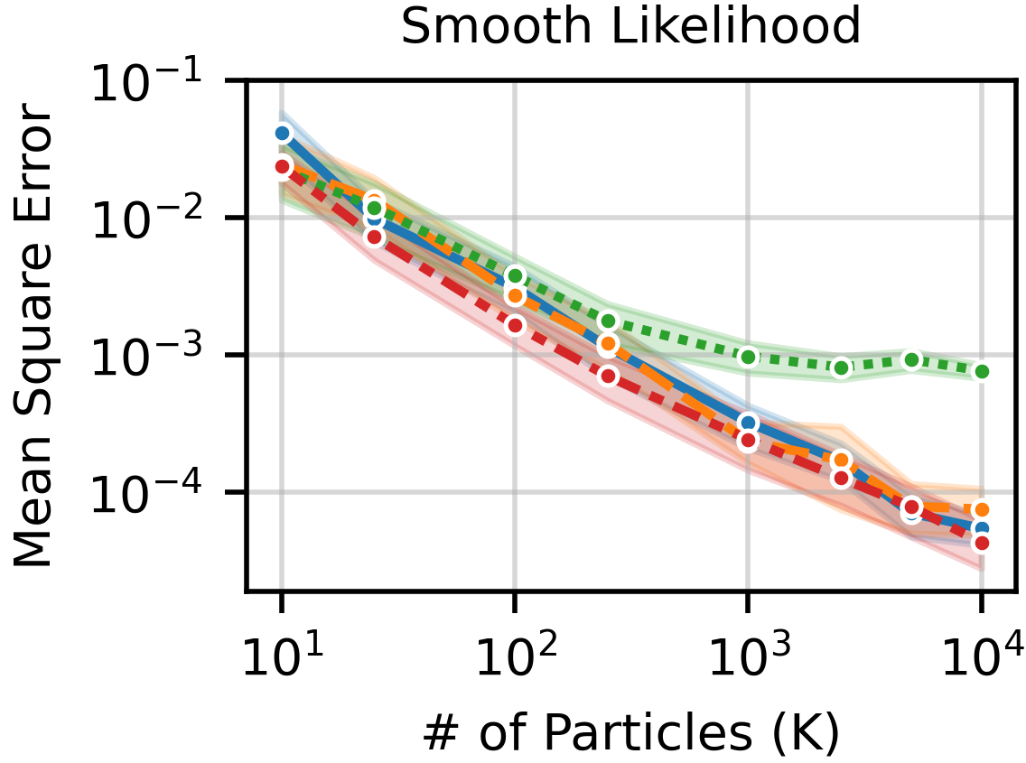
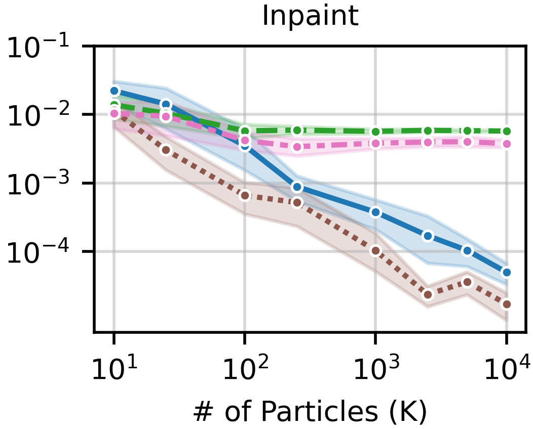
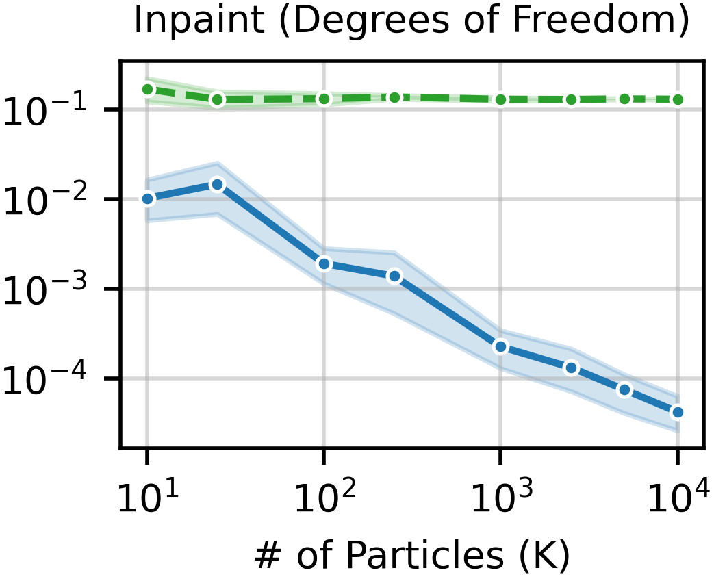
Figure E: Errors of conditional mean estimations with 2 SEM error bars averaged over 25 replicates on mixture of Gaussians unconditional target. TDS applies to all three tasks and provides increasing accuracy with more particles.

Forward process.

Our forward process is variance preserving (as described in Appendix A) with $T=100$ steps and a quadratic variance schedule. We set $\sigma^{2}_{t}=\sigma^{2}_{\mathrm{min}}+(\frac{t}{T})^{2}\sigma^{2}_{\mathrm{max}}$ with $\sigma^{2}_{\mathrm{min}}=10^{-5}$ and $\sigma^{2}_{\mathrm{max}}=10^{-1}.$

Unconditional target distributions and likelihood.

We evaluate the different methods with two different unconditional target distributions:

1. A bivariate Gaussian with mean at $(\frac{1}{2},\frac{1}{2})$ and covariance $0.9$ and

2. A Gaussian mixture with three components with mixing proportions $[0.3,0.5,0.2],$ means $[(1.54,-0.29),(-2.18,0.57),(-1.09,-1.40)]$, and $0.2$ standard deviations.

We evaluate on conditional distributions defined by the three likelihoods described in Section 5.1.

Figure E provides results analogous to those in Figure 1 but with the mixture of Gaussians unconditional target. In this second example we evaluate a with a variation of the inpainting degrees of freedom case wherein we consider $y=1$ and $\mathcal{M}=\{[1],[2]\},$ so that $p_{y|x^{0}}({y}|{x^{0}})=\delta_{y}(x^{0}_{1})+\delta_{y}(x^{0}_{2}).$

C.2 MNIST experiments

Setup.

We set up an MNIST diffusion model using variance preserving framework. The model architecture is based on the guided diffusion codebase with the following specifications: number of channels = 64, attention resolutions = "28,14,7", number of residual blocks = 3, learn sigma (i.e. to learn the variance of $p_{\theta}(x^{t-1}~{}|~{}x^{t})$) = True, resblock updown = True, dropout = 0.1, variance schedule = "linear". We trained the model for 60k epochs with a batch size of 128 and a learning rate of $10^{-4}$ on 60k MNIST training images. The model uses $T=1000$ for training and $T=100$ for sampling.

The classifier used for class-conditional generation and evaluation is a pretrained ResNet50 model. This classifier is trained on the same set of MNIST training images used by diffusion model training.

C.2.1 MNIST class-conditional generation

Sample plots.

To supplement the sample plot conditioned on class $7$ in Figure 2(a), we present samples conditioned on each of the remaining 9 classes. These results exhibit the same characteristics of relative diversity and quality discussed in Section 5.2.

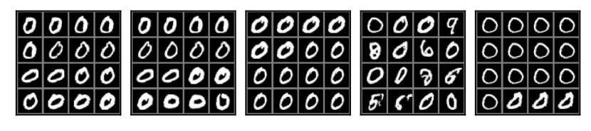
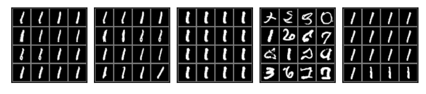
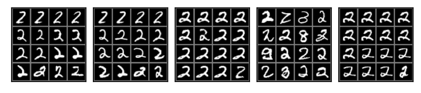
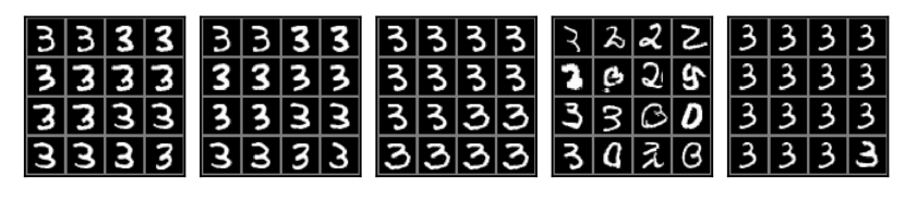
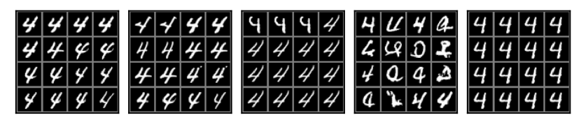
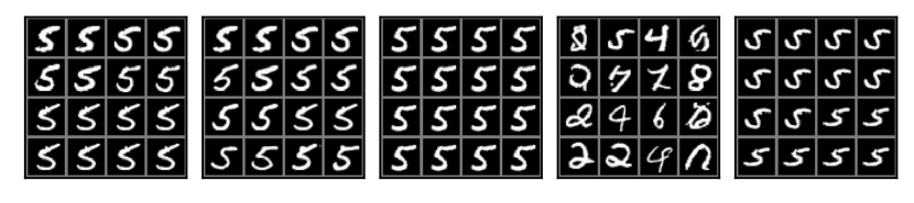
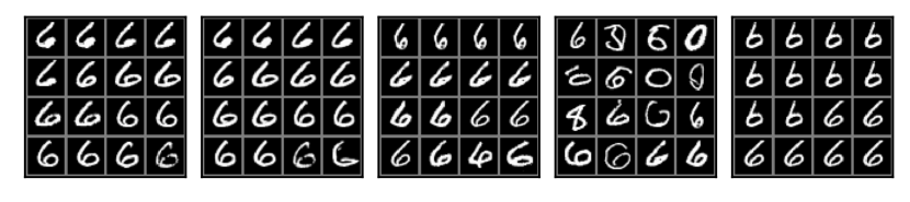
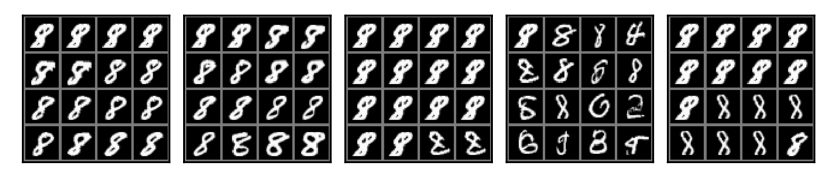
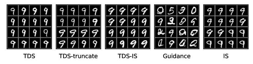
Figure F: MNIST class-conditional generation. 16 randomly chosen conditional samples from 64 particles in a single run, given class $y$. From top to bottom, $y=0,1,2,3,4,5,6,8,9$.

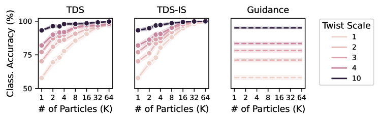
(a) Classification accuracy (measured by the neural network classifier) v.s. number of particles $K$, under different twist scales. Results are averaged over 1,000 random runs with error bands indicating 2 standard errors. Across the panels we see that for all the methods, the larger the twist scale (i.e. the darker the line color), the higher the classification accuracy. For TDS and TDS-IS, this improvement is more significant for smaller value of $K$,

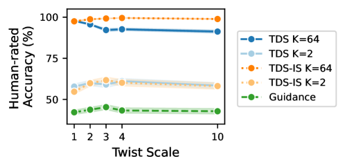
(b) Human-rated classification accuracy v.s. twist scale, for TDS ($K=64,2$), TDS-IS ($K=64,2$) and Guidance. Results are averaged over 640 randomly chosen samples with error bands indicating 2 standard errors. For TDS ($K=2$), TDS-IS ($K=64,2$) and Guidance, a moderate increase in twist scale improves the human-rated accuracy; however, excessively large twist scale can hurt the accuracy. For TDS ($K=64$), increasing the twist scale generally decreases the human-rated accuracy.

Figure G: MNIST class-conditional generation: classification accuracy under different twist scales, computed by a neural network classifier (top panel) and a human (bottom panel).

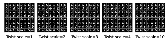
(a) TDS ($K=64$). # of good-quality samples counted by human is 62, 61, 63, 60, 62, from left to right.

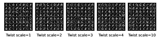
(b) TDS ($K=2$). # of good-quality samples counted by human 49, 51, 51, 46, 45, from left to right.

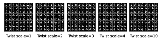
(c) TDS-IS ($K=64$). # of good-quality samples counted by a human is 62, 61, 64, 64, 61, from left to right.

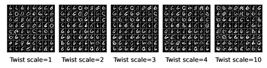
(d) TDS-IS ($K=2$). # of good-quality samples counted by a human is 49, 52, 53, 52, 48, from left to right.

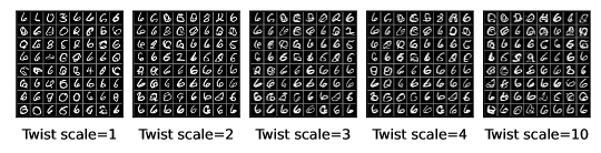
(e) Guidance. # of good-quality samples counted by a human is 31, 38, 41, 39, 34, from left to right.

Figure H: MNIST class-conditional generation: random samples selected from 64 random runs conditioned on class 6 under different twist scales. Top to bottom: TDS ($K=64$), TDS ($K=2$), TDS-IS ($K=64$), TDS-IS ($K=2$) and Guidance. In general, moderately large twist scales improve the sample quality. However, overly large twist scale (e.g. 10) would distort the digit shape with more artifacts, though retaining useful features that may allow a neural network classifier to identity the class.

Ablation study on twist scales.

We consider exponentiating and re-normalizing twisting functions by a twist scale $\gamma$, i.e. setting new twisting functions to $\tilde{p}_{\theta}(y~{}|~{}x^{t};\gamma)\propto p_{y|x^{0}}({y}|{{\hat{x}}_{\theta}(x^{t})})^{\gamma}$. In particular, when $t=0$, we set $p_{y|x^{0}}({y}|{x^{0};\gamma})\propto p_{y|x^{0}}({y}|{x^{0}})^{\gamma}$. This modification suggests that the targeted conditional distribution is now

$$p_{\theta}(x^{0}~{}|~{}y;\gamma)\propto p_{\theta}(x^{0})p_{y|x^{0}}({y}|{x^{0}})^{\gamma}.$$ (63)

By setting $\gamma>1$, the classification likelihood becomes sharper, which is potentially helpful for twisting the samples towards a specific class. The TDS algorithm (and likewise TDS-IS and Guidance) still apply with this new definition of twisting functions. The use of twist scale is similar to the classifier scale introduced in classifier-guidance literature, which is used to multiply the gradient of the log classification probability [8].

In Figure G, we examine the effect of varying twist scales on classification accuracy of TDS, TDS-IS and Guidance. We consider two ways to evaluate the accuracy. First, classification accuracy computed by a neural network classifier, where the evaluation setup is the same as in Section 5.2. Second, the human-rated classification accuracy, where a human (one of the authors) checks if a generated digit has the right class and does not have artifacts. Since human evaluation is expensive, we only evaluate TDS, TDS-IS (both with $K=64,2$) and Guidance. In each run, we randomly sample one particle out of $K$ particles according to the associated weights. We conduct 64 runs for each class label, leading to a total of 640 samples for human evaluation.

Figure 7(a) depicts the classification accuracy measured by a neural network classifier. We observe that in general larger twist scale improves the classification accuracy. For TDS and TDS-IS, the improvement is more significant for smaller number of particles $K$ used.

Figure 7(b) depicts the human-rated accuracy. In this case, we find that larger twist scale is not necessarily better. A moderately large twist scale ($\gamma=2,3$) generally helps increasing the accuracy, while an excessively large twist scale ($\gamma=10$) decreases the accuracy. An exception is TDS with $K=64$ particles, where any $\gamma>1$ leads to worse accuracy compared to the case of $\gamma=1$. Study on twist scale aside, we find that using more particles $K$ help improving human-rated accuracy (recall that Guidance is a special case of TDS with $K=1$): given the same twist scale, TDS with $K=1,2,64$ has increasing accuracy. In addition, both TDS and TDS-IS with $K=64$ and $\gamma=1$ have almost perfect accuracy. The effect of $K$ on human-rated accuracy is consistent with previous findings with neural network classifier evaluation in Section 5.2.

We note that there is a discrepancy on the effects of twist scales between neural network evaluation and human evaluation. We suspect that when overly large twist scale is used, the generated samples may fall out of the data manifold; however, they may still retain features recognizable to a neural network classifier, thereby leading to a low human-rated accuracy but a high classifier-rated accuracy. To validate this hypothesis, we present samples conditioned on class 6 in Figure H. For example, in Figure 8(e), Guidance with $\gamma=1$ has 31 good-quality samples out of 64, and the rest of the samples often resamble the shape of other digits, e.g. 3,4,8; and Guidance with $\gamma=10$ has 34 good-quality samples, but most of the remaining samples resemble 6 with many artifacts.

C.2.2 MNIST inpainting

The inpainting task is to sample images from $p_{\theta}(x^{0}~{}|~{}x^{0}_{\mathbf{M}}=y)$ given observed part $x^{0}_{\mathbf{M}}=y$. Here we segment $x^{0}=[x^{0}_{\mathbf{M}},x^{0}_{\mathbf{\bar{M}}}]$ into observed dimensions $\mathbf{M}$ and unobserved dimensions $\mathbf{\bar{M}}$, as described in Section 3.3.

In this experiment, we consider two types of observed dimensions: (1) $\mathbf{M}$ = “half”, where the left half of an image is observed, and (2) $\mathbf{M}$ = “quarter”, where the upper left quarter of an image is observed.

We run TDS, TDS-IS, Guidance, SMC-Diff, and Replacement to inpaint 10,000 validation images. We also include TDS-truncate that truncates the TDS procedure at $t=10$ and returns ${\hat{x}}_{\theta}(x^{10})$.

Similar to the class-conditional generation task, we can use twist scale $\gamma_{t}$ to exponentiate the twisting functions. In the inpainting case, it is equivalent to multiplying the variance of the twisting function defined in eq. 18 by $\gamma_{t}$. Denote the new variance by $\tilde{\gamma}_{t}$. By default TDS sets $\tilde{\gamma}_{t}:=(\tilde{\sigma}_{t}^{2}\tau^{2})/(\tilde{\sigma}_{t}^{2}+\tau^{2})$, where $\tilde{\sigma}_{t}^{2}:=(1-\bar{\alpha}_{t})/\bar{\alpha}_{t}$ and $\tau^{2}=0.12$ is the population variance of $x^{0}$ estimated from training data.

Metrics.

As in Section 5.2, we use effective sample size (ESS) to compare the particle efficiency among different SMC samplers (namely TDS, TDS-IS, and SMC-Diff).

In addition, we ground the performance of a sampler in the downstream task of classifying a partially observed image $x^{0}_{\mathbf{M}}=y$: we use a classifier to predict the class $\hat{z}$ of an inpainted image $x^{0}$, and compute the accuracy against the true class $z^{*}$ of the unmasked image ($z^{*}$ is provided in MNIST dataset). This prediction is made by the same classifier used in Section 5.2.

Consider $K$ weighted particles $\{x^{0}_{k};w^{0}_{k}\}_{k=1}^{K}$ drawn from a sampler conditioned on $x^{0}_{\mathbf{M}}=y$ and assume the weights are normalized. We define the Bayes accuracy (BA) as

$$\mathds{1}\left\{\hat{z}(y)=z^{*}\right\},\quad\mathrm{with}\quad\hat{z}(y):=\operatorname*{arg\,max}_{z=1:10}\sum_{k=1}^{K}w^{0}_{k}p(z;x^{0}_{k}),$$ (64)

where $\hat{z}(y)$ is viewed as an approximation to the Bayes optimal classifier $\hat{z}^{*}(y)$ given by

$$\begin{split}\hat{z}^{*}(y)&:=\operatorname*{arg\,max}_{z=1:10}p_{\theta}(z~{}|~{}x^{0}_{\mathbf{M}}=y)=\operatorname*{arg\,max}_{z=1:10}\int p_{\theta}(x^{0}~{}|~{}x^{0}_{\mathbf{M}}=y)p(z;x^{0})dx^{0}.\end{split}$$ (65)

(In eq. 65 we assume the classifier $p_{y|x^{0}}({\cdot}|{x^{0}})$ is the optimal classifier on full images.)

We also consider classification accuracy (CA) defined as the following

$$\sum_{k=1}^{K}w^{0}_{k}\mathds{1}\{\hat{z}(x^{0}_{k})=z^{*}\},\quad\mathrm{with}\quad\hat{z}(x^{0}_{k}):=\operatorname*{arg\,max}_{z=1:10}p_{y|x^{0}}({z}|{x^{0}_{k}}).$$ (66)

BA and CA evaluate different aspects of a sampler. BA is focused on the optimal prediction among multiple particles, whereas CA is focused on the their weighted average prediction.

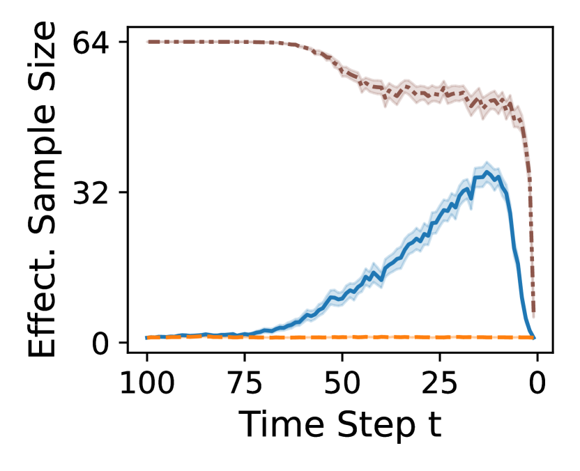
(a) $\mathbf{M}$ = “half”. ESS trace.

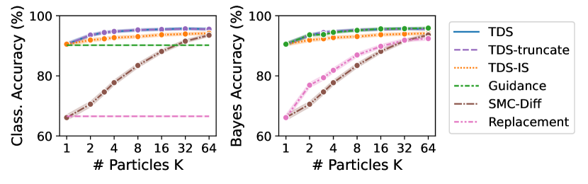
(b) $\mathbf{M}$ = “half”. Class. accuracy (left), and Bayes accuracy (right) v.s. $K$.

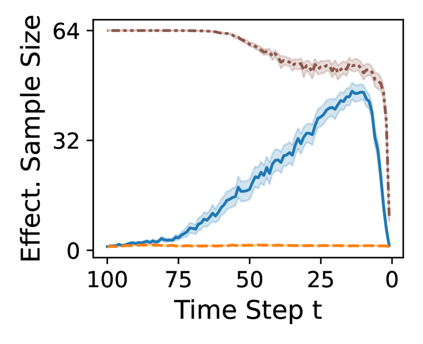
(c) $\mathbf{M}$ = “quarter”. ESS trace.

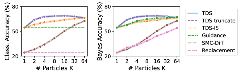
(d) $\mathbf{M}$ = “quarter”. Class. accuracy (left), and Bayes accuracy (right) v.s. $K$.

Figure I: MNIST image inpainting. Results for observed dimension $\mathbf{M}$ = “half” are shown in the top panel, and $\mathbf{M}$ = “quarter” in the bottom panel. (i) Left column: ESS traces are averaged over 100 different images inpainted by TDS, TDS-IS, and SMC-Diff, all with $K=64$ particles. TDS’s ESS is generally increasing untill the final 20 steps where it drops to around 1, suggesting significant particle collapse in the end of generation trajectory. TDS-IS’s ESS is always around 1. SMC-Diff has higher particle efficiency compared to TDS. (ii) Right column: Classification accuracy and Bayes accuracy are averaged over 10,000 images. In general increasing the number of particles $K$ would improve the performance of all samplers. TDS and TDS-truncate have the highest accuracy among all given the same $K$. (iii) Finally, comparison of top and bottom panels shows that in a harder inpainting problem where $\mathbf{M}$ = “quarter”, TDS’s has a higher ESS but lower CA and BA.

Comparison results of different methods.

Figure I depicts the ESS trace, BA and CA for different samplers. The overall observations are similar to the observations in the class-conditional generation task in Section 5.2, except that SMC-Diff and Replacement methods are not available there.

Replacement has the lowest CA and BA across all settings. Comparing TDS to SMC-Diff, we find that SMC-Diff’s ESS is consistently greater than TDS; however, SMC-Diff is outperformed by TDS in terms of both CA and BA.

We also note that despite Guidance’s CA is lower, its BA is comparable to TDS. This result is due to that as long as Guidance generates a few good-quality samples out of $K$ particles, the optimal prediction can be accurate, thereby resulting in a high BA.

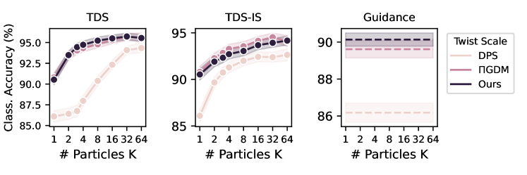
(a) $\mathbf{M}$ = “half”. Classification accuracy under different twist scale schemes.

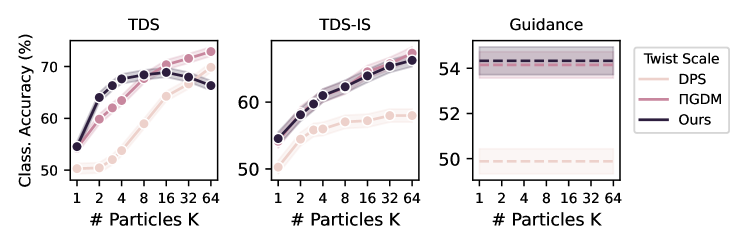
(b) $\mathbf{M}$ = “quarter”. Classification accuracy under different twist scale schemes.

Figure J: MNIST image inpainting: Ablation study on twist scales. Top: observed dimensions $\mathbf{M}$ = “half”. Bottom: $\mathbf{M}$ = “quarter”. In most case, the performance of our choice of twist scale is similar to that of $\Pi$GDM, and is better compared to DPS.

Ablation study on twist scales.

We compare the following three twist scale schemes that define the variance of twisting functions:

1. DPS: $\tilde{\gamma}_{t}:=2\|{\hat{x}}_{\theta}(x^{t})_{\mathbf{M}}-y\|_{2}\sigma_{t}^{2}$, adapted from [5] (see Algorithm 1).

2. $\Pi$GDM: $\tilde{\gamma}_{t}:=\sigma_{t}^{2}/\sqrt{\bar{\alpha}_{t}}$, adapted from [27] (see Algorithm 1).

3. TDS scaling: $\tilde{\gamma}_{t}:=\tilde{\sigma}_{t}^{2}\tau^{2}/\tilde{\sigma}_{t}^{2}+\tau^{2}$ where $\tilde{\sigma}_{t}^{2}:=(1-\bar{\alpha}_{t})/\bar{\alpha}_{t}$ and $\tau^{2}=0.12$ is the population variance of $x^{0}$ estimated from training data.

Figure J shows the classification accuracy of TDS, TDS-IS and Guidance with different twist scale schemes. We find that our choice has similar performance to that of $\Pi$GDM, and outperforms DPS in most cases. Exceptions are when $\mathbf{M}$ = “quarter” and for large $K$, TDS with twist scale choice of $\Pi$GDM or DPS has higher CA, as is shown in the left panel in Figure 10(b).

Appendix D Motif-scaffolding application details

Unconditional model of protein backbones. We here use the FrameDiff, a diffusion generative model described by Yim et al. [34]. FrameDiff parameterizes protein $N$-residue protein backbones as a collection of rigid bodies defined by rotations and translations as $x^{0}=[(R_{1},z_{1}),\dots,(R_{N},z_{N})]\in SE(3)^{N}$. $SE(3)$ is the special Euclidean group in three dimensions (a Riemannian manifold). Each $R_{n}\in SO(3)$ (the special orthogonal group in three dimensions) is a rotation matrix and each $z_{n}\in\mathbb{R}^{3}$ in a translation. Together, $R_{n}$ and $z_{n}$ describe how one obtains the coordinates of the three backbone atoms C, $\texttt{C}_{\alpha}$, and N for each residue by translating and rotating the coordinates of an idealized residue with $C_{\alpha}$ carbon and the origin. The conditioning information is then a motif $y=x^{0}_{\mathbf{M}}\in SE(3)^{|\mathbf{M}|}$ for some $\mathbf{M}\subset\{1,\dots,N\}.$ FrameDiff is a continuous time diffusion model and includes the number of steps as a hyperparmeter; we use 200 steps in all experiments. We refer the reader to [34] for details on the neural network architecture, and details of the forward and reverse diffusion process.

Evaluation details.

For our self-consistency evaluation we use ProteinMPNN [6] with default settings to generate 8 sequences for each sampled backbone. Positions not indicated as resdesignable in [32, Methods Table 9] are held fixed. We use AlphaFold [17] for forward folding. We define a “success” as a generated backbones for which at least one of the 8 sequences has backbone atom with both scRMSD < 1 Å on the motif and scRMSD < 2 Å on the full backbone. We benchmarked TDS on 24/25 problems in the benchmark set introduced [32, Methods Table 9]. A 25th problem (6VW1) is excluded because it involves multiple chains, which cannot be represented by FrameDiff. Because FrameDiff requires specifying a total length of scaffolds. In all replicates, we fixed the scaffold the median of the Total Length range specified by Watson et al. [32, Methods Table 9]. For example, 116 becomes 125 and 62-83 becomes 75.

D.1 Additional Results

Impact of twist scale on additional motifs.

Figure 3 showed monotonically increasing success rates with the twist scale. However, this trend does not hold for every problem. LABEL:{fig:prot-twist-scale} demonstrates this by comparing the success rates with different twist-scales on five additional benchmark problems.

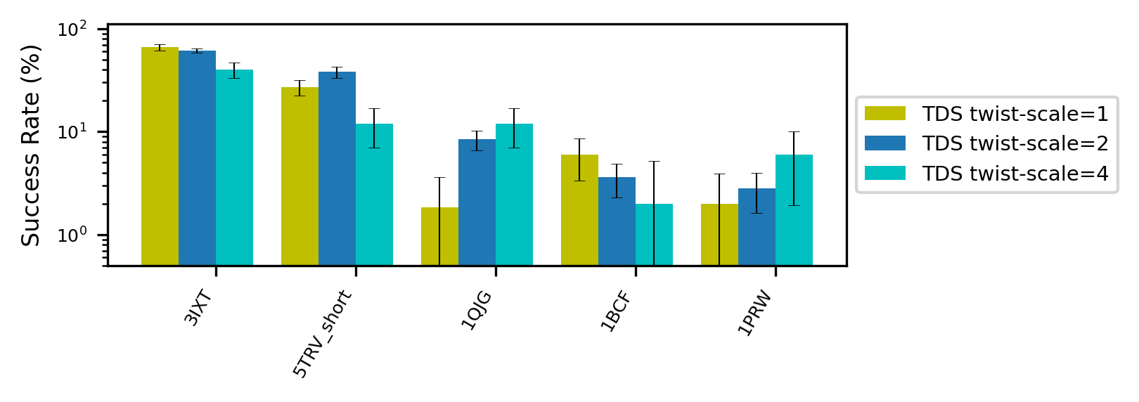
Figure K: Increasing the twist scale has a different impact across motif-scaffolding benchmark problems.

Effective sample size varies by problem.

Figure L shows two example effective sample size traces over the course of sample generation. For 6EXZ-med resampling was triggered 38 times (with 14 in the final 25 steps), and for 5UIS resampling was triggered 63 times (with 13 in the final 25 steps). The traces are representative of the larger benchmark.

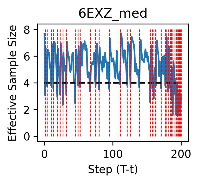
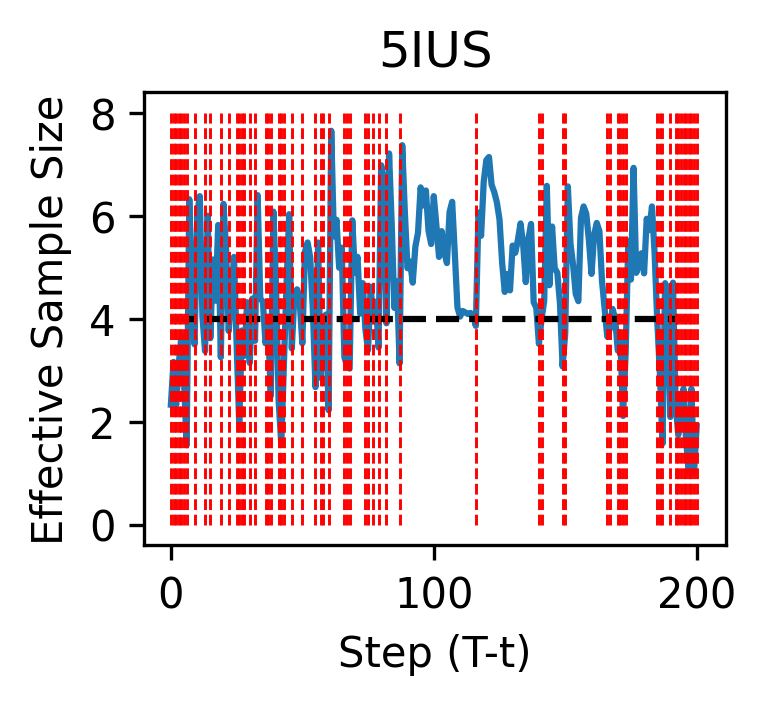
Figure L: Effective sample size traces for two motif-scaffolding examples (Left) 6EXZ-med and (Right) 5IUS. In both case $K=8$ and a resampling threshold of $0.5K$ is used. Dashed red lines indicate resampling times.

Application of TDS to RFdiffusion:

We also tried applying TDS to RFdiffusion [32]. RFdiffusion is a diffusion model that uses the same backbone structure representation as FrameDiff. However, unlike FrameDiff, RFdiffusion trained with a mixture of conditional examples, in which a segment of the backbone is presented as input as a desired motif, and unconditional training examples in which the only a noised backbone is provided. Though in our benchmark evaluation provided the motif information as explicit conditioning inputs, we reasoned that TDS should apply to RFdiffusion as well (with conditioning information not provided as input). However, we were unable to compute numerically stable gradients (with respect to either the rotational or translational components of the backbone representation); this lead to twisted proposal distributions that were similarly unstable and trajectories that frequently diverged even with one particle. We suspect this instability owes to RFdiffusion’s structure prediction pretraining and limited fine-tuning, which may allow it to achieve good performance without having fit a smooth score-approximation.

References

- Bansal et al. [2023] Arpit Bansal, Hong-Min Chu, Avi Schwarzschild, Soumyadip Sengupta, Micah Goldblum, Jonas Geiping, and Tom Goldstein. Universal guidance for diffusion models. arXiv preprint arXiv:2302.07121, 2023.
- Chatterjee and Diaconis [2018] Sourav Chatterjee and Persi Diaconis. The sample size required in importance sampling. The Annals of Applied Probability, 28(2):1099–1135, 2018.
- Chirikjian and Kobilarov [2014] Gregory Chirikjian and Marin Kobilarov. Gaussian approximation of non-linear measurement models on lie groups. In 53rd IEEE Conference on Decision and Control, pages 6401–6406. IEEE, 2014.
- Chopin and Papaspiliopoulos [2020] Nicolas Chopin and Omiros Papaspiliopoulos. An introduction to sequential Monte Carlo. Springer, 2020.
- Chung et al. [2023] Hyungjin Chung, Jeongsol Kim, Michael T Mccann, Marc L Klasky, and Jong Chul Ye. Diffusion posterior sampling for general noisy inverse problems. In International Conference on Learning Representations, 2023.
- Dauparas et al. [2022] Justas Dauparas, Ivan Anishchenko, Nathaniel Bennett, Hua Bai, Robert J Ragotte, Lukas F Milles, Basile IM Wicky, Alexis Courbet, Rob J de Haas, Neville Bethel, , Philip J Leung, Timothy Huddy, Sam Pellock, Doug Tischer, F Chan, Brian Koepnick, H Nguyen, Alex Kang, B Sankaran, Asim K. Bera, Neil P. King, and David Baker. Robust deep learning-based protein sequence design using ProteinMPNN. Science, 378(6615):49–56, 2022.
- De Bortoli et al. [2022] Valentin De Bortoli, Emile Mathieu, Michael John Hutchinson, James Thornton, Yee Whye Teh, and Arnaud Doucet. Riemannian score-based generative modelling. In Advances in Neural Information Processing Systems, 2022.
- Dhariwal and Nichol [2021] Prafulla Dhariwal and Alexander Nichol. Diffusion models beat GANs on image synthesis. Advances in Neural Information Processing Systems, 2021.
- Doucet et al. [2001] Arnaud Doucet, Nando De Freitas, and Neil James Gordon. Sequential Monte Carlo methods in practice, volume 1. Springer, 2001.
- Du et al. [2023] Yilun Du, Conor Durkan, Robin Strudel, Joshua B Tenenbaum, Sander Dieleman, Rob Fergus, Jascha Sohl-Dickstein, Arnaud Doucet, and Will Grathwohl. Reduce, reuse, recycle: Compositional generation with energy-based diffusion models and mcmc. arXiv preprint arXiv:2302.11552, 2023.
- Gordon et al. [1993] Neil J Gordon, David J Salmond, and Adrian FM Smith. Novel approach to nonlinear/non-Gaussian Bayesian state estimation. In IEE proceedings F (radar and signal processing), volume 140, pages 107–113. IET, 1993.
- Guarniero et al. [2017] Pieralberto Guarniero, Adam M Johansen, and Anthony Lee. The iterated auxiliary particle filter. Journal of the American Statistical Association, 112(520):1636–1647, 2017.
- Heng et al. [2020] Jeremy Heng, Adrian N Bishop, George Deligiannidis, and Arnaud Doucet. Controlled sequential Monte Carlo. Annals of Statistics, 48(5), 2020.
- Ho and Salimans [2022] Jonathan Ho and Tim Salimans. Classifier-free diffusion guidance. arXiv preprint arXiv:2207.12598, 2022.
- Ho et al. [2020] Jonathan Ho, Ajay Jain, and Pieter Abbeel. Denoising diffusion probabilistic models. In Advances in Neural Information Processing Systems, 2020.
- Ho et al. [2022] Jonathan Ho, Tim Salimans, Alexey A Gritsenko, William Chan, Mohammad Norouzi, and David J Fleet. Video diffusion models. In Advances in Neural Information Processing Systems, 2022.
- Jumper et al. [2021] John M. Jumper, Richard Evans, Alexander Pritzel, Tim Green, Michael Figurnov, Olaf Ronneberger, Kathryn Tunyasuvunakool, Russ Bates, Augustin Zídek, Anna Potapenko, Alex Bridgland, Clemens Meyer, Simon A A Kohl, Andy Ballard, Andrew Cowie, Bernardino Romera-Paredes, Stanislav Nikolov, Rishub Jain, Jonas Adler, Trevor Back, Stig Petersen, David A. Reiman, Ellen Clancy, Michal Zielinski, Martin Steinegger, Michalina Pacholska, Tamas Berghammer, Sebastian Bodenstein, David Silver, Oriol Vinyals, Andrew W. Senior, Koray Kavukcuoglu, Pushmeet Kohli, and Demis Hassabis. Highly accurate protein structure prediction with AlphaFold. Nature, 596(7873):583 – 589, 2021.
- Karras et al. [2022] Tero Karras, Miika Aittala, Timo Aila, and Samuli Laine. Elucidating the design space of diffusion-based generative models. arXiv preprint arXiv:2206.00364, 2022.
- Kawar et al. [2022] Bahjat Kawar, Michael Elad, Stefano Ermon, and Jiaming Song. Denoising diffusion restoration models. arXiv preprint arXiv:2201.11793, 2022.
- Lugmayr et al. [2022] Andreas Lugmayr, Martin Danelljan, Andres Romero, Fisher Yu, Radu Timofte, and Luc Van Gool. Repaint: Inpainting using denoising diffusion probabilistic models. In Proceedings of the IEEE/CVF Conference on Computer Vision and Pattern Recognition, pages 11461–11471, 2022.
- Meng et al. [2021] Chenlin Meng, Yutong He, Yang Song, Jiaming Song, Jiajun Wu, Jun-Yan Zhu, and Stefano Ermon. SDEdit: Guided image synthesis and editing with stochastic differential equations. In International Conference on Learning Representations, 2021.
- Naesseth et al. [2019] Christian A Naesseth, Fredrik Lindsten, and Thomas B Schön. Elements of sequential Monte Carlo. Foundations and Trends in Machine Learning, 12(3):307–392, 2019.
- Ramesh et al. [2022] Aditya Ramesh, Prafulla Dhariwal, Alex Nichol, Casey Chu, and Mark Chen. Hierarchical text-conditional image generation with clip latents. arXiv preprint arXiv:2204.06125, 2022.
- Saharia et al. [2022a] Chitwan Saharia, William Chan, Huiwen Chang, Chris Lee, Jonathan Ho, Tim Salimans, David Fleet, and Mohammad Norouzi. Palette: Image-to-image diffusion models. In ACM SIGGRAPH 2022 Conference Proceedings, pages 1–10, 2022a.
- Saharia et al. [2022b] Chitwan Saharia, Jonathan Ho, William Chan, Tim Salimans, David J Fleet, and Mohammad Norouzi. Image super-resolution via iterative refinement. IEEE Transactions on Pattern Analysis and Machine Intelligence, 2022b.
- Shi et al. [2022] Yuyang Shi, Valentin De Bortoli, George Deligiannidis, and Arnaud Doucet. Conditional simulation using diffusion Schrödinger bridges. In Uncertainty in Artificial Intelligence, 2022.
- Song et al. [2023] Jiaming Song, Arash Vahdat, Morteza Mardani, and Jan Kautz. Pseudoinverse-guided diffusion models for inverse problems. In International Conference on Learning Representations, 2023.
- Song et al. [2020] Yang Song, Jascha Sohl-Dickstein, Diederik P Kingma, Abhishek Kumar, Stefano Ermon, and Ben Poole. Score-based generative modeling through stochastic differential equations. International Conference on Learning Representations, 2020.
- Trippe et al. [2023] Brian L Trippe, Jason Yim, Doug Tischer, Tamara Broderick, David Baker, Regina Barzilay, and Tommi Jaakkola. Diffusion probabilistic modeling of protein backbones in 3D for the motif-scaffolding problem. In International Conference on Learning Representations, 2023.
- Vincent [2011] Pascal Vincent. A connection between score matching and denoising autoencoders. Neural computation, 23(7):1661–1674, 2011.
- Wang et al. [2022] Jue Wang, Sidney Lisanza, David Juergens, Doug Tischer, Joseph L Watson, Karla M Castro, Robert Ragotte, Amijai Saragovi, Lukas F Milles, Minkyung Baek, et al. Scaffolding protein functional sites using deep learning. Science, 377(6604), 2022.
- Watson et al. [2022] Joseph L. Watson, David Juergens, Nathaniel R. Bennett, Brian L. Trippe, Jason Yim, Helen E. Eisenach, Woody Ahern, Andrew J. Borst, Robert J. Ragotte, Lukas F. Milles, Basile I. M. Wicky, Nikita Hanikel, Samuel J. Pellock, Alexis Courbet, William Sheffler, Jue Wang, Preetham Venkatesh, Isaac Sappington, Susana Vázquez Torres, Anna Lauko, Valentin De Bortoli, Emile Mathieu, Regina Barzilay, Tommi S. Jaakkola, Frank DiMaio, Minkyung Baek, and David Baker. Broadly applicable and accurate protein design by integrating structure prediction networks and diffusion generative models. bioRxiv, 2022.
- Whiteley and Lee [2014] Nick Whiteley and Anthony Lee. Twisted particle filters. The Annals of Statistics, 42(1):115–141, 2014.
- Yim et al. [2023] Jason Yim, Brian L Trippe, Valentin De Bortoli, Emile Mathieu, Arnaud Doucet, Regina Barzilay, and Tommi Jaakkola. SE (3) diffusion model with application to protein backbone generation. In International Conference on Machine Learning, 2023.
- Zhang et al. [2023] Guanhua Zhang, Jiabao Ji, Yang Zhang, Mo Yu, Tommi Jaakkola, and Shiyu Chang. Towards coherent image inpainting using denoising diffusion implicit models. arXiv preprint arXiv:2304.03322, 2023.