Precision Anti-Cancer Drug Selection via Neural Ranking

Abstract.

Personalized cancer treatment requires a thorough understanding of complex interactions between drugs and cancer cell lines in varying genetic and molecular contexts. To address this, high-throughput screening has been used to generate large-scale drug response data, facilitating data-driven computational models. Such models can capture complex drug-cell line interactions across various contexts in a fully data-driven manner. However, accurately prioritizing the most sensitive drugs for each cell line still remains a significant challenge. To address this, we developed neural ranking approaches that leverage large-scale drug response data across multiple cell lines from diverse cancer types. Unlike existing approaches that primarily utilize regression and classification techniques for drug response prediction, we formulated the objective of drug selection and prioritization as a drug ranking problem. In this work, we proposed two neural listwise ranking methods that learn latent representations of drugs and cell lines, and then use those representations to score drugs in each cell line via a learnable scoring function. Specifically, we developed a neural listwise ranking method, $\mathop{\mathtt{List\text{-}One}}\limits$, on top of the existing method ListNet. Additionally, we proposed a novel listwise ranking method, $\mathop{\mathtt{List\text{-}All}}\limits$, that focuses on all the sensitive drugs instead of the top sensitive drug, unlike $\mathop{\mathtt{List\text{-}One}}\limits$. Our results demonstrate that $\mathop{\mathtt{List\text{-}All}}\limits$ outperforms the best baseline with significant improvements of as much as 8.6% in hit@20 across 50% test cell lines. Furthermore, our analyses suggest that the learned latent spaces from our proposed methods demonstrate informative clustering structures and capture relevant underlying biological features. Moreover, our comprehensive empirical evaluation provides a thorough and objective comparison of the performance of different methods (including our proposed ones).

1. Introduction

Precision cancer treatment aims to tailor therapies to individual patients by identifying effective anti-cancer drugs for each patient based on their unique genetic and molecular characteristics. However, this requires an in-depth understanding of complex interactions between drugs and patients in different genetic and molecular contexts, which presents a significant challenge. To address this challenge, high-throughput screening methods(Gupta et al., 2009) have been used to generate large-scale drug response data(Yang et al., 2012; Barretina et al., 2012), providing a valuable resource for developing data-driven models. However, developing models that can accurately encode complex interactions between cell lines and drugs and prioritize the most promising anti-cancer drugs for each cell line still remains a challenging task. To tackle these challenges, data-driven models jointly utilize drug response data across multiple cell lines and cancer types, motivated by findings from pan-cancer studies(Weinstein et al., 2013). These studies suggest that there are commonalities in genetic and molecular features among different cancer types(Kandoth et al., 2013). Following such insights, in this paper, we develop computational approaches that can leverage drug response data across a large number of cell lines from diverse cancer types to identify and prioritize anti-cancer drugs in each cell line. Unlike existing computational approaches, our approach is inspired by learning-to-rank (LeToR) methods(Burges et al., 2005), which can naturally formulate the objective of anti-cancer drug selection and prioritization.

In this work, we develop neural listwise LeToR methods that learn latent representations of cell lines and drugs in a data-driven manner, and then use those representations to score drugs in each cell line via a learnable scoring function. We utilize the existing listwise ranking objective(Cao et al., 2007) to develop a neural listwise ranking method, denoted as $\mathop{\mathtt{List\text{-}One}}\limits$, which considers the entire ranking structure at a time and learns the probability of the most sensitive drugs in each cell line being ranked at the top (i.e., top-one probability distribution). By minimizing the discrepancy between the predicted and ground-truth top-one probability distributions, $\mathop{\mathtt{List\text{-}One}}\limits$ learns to appropriately score the drugs leading to an accurate selection of the most sensitive drug in each cell line.

In addition, we propose another listwise ranking method for drug selection, denoted as $\mathop{\mathtt{List\text{-}All}}\limits$, that focuses on selecting all the sensitive drugs. Additionally, we evaluated our proposed methods against strong regression and pairwise ranking baselines. Our results demonstrate that $\mathop{\mathtt{List\text{-}All}}\limits$ mostly outperforms the best baselines with significant improvements of much as 8.6% in hit@20 across 50% test cell lines. Furthermore, our analyses suggest that the learned latent spaces from our proposed methods demonstrate informative clustering structures and capture relevant underlying biological features (e.g., cancer types, drug mechanism of action).

The rest of the manuscript is organized as follows. Section 2 presents the related work on computational methods in anti-cancer drug response prediction and drug prioritization. Section 3 presents the proposed listwise methods and Section 4 describes the datasets, baseline methods, experimental settings and evaluation metrics. Section 5 presents an overall comparison of all methods in one experimental setting across both datasets and detailed analyses of embeddings. Section 6 concludes the paper.

2. Related Works

2.1. Computational Methods in Drug Response Prediction

With an increasing abundance of large-scale drug response data and advanced high-throughput screening(Gupta et al., 2009), data-driven computational approaches have been developed for drug response prediction in cancer cell lines. Following pan-cancer studies(Weinstein et al., 2013), these approaches have been extended beyond singe-drug or single-cell line modeling to jointly leverage the drug response data across multiple drugs and cell lines. This enables such approaches to capture the interactions among multiple drugs, among multiple cell lines, and between drugs and cell lines. Typically, these approaches either focus on regression(Su et al., 2019) which estimates the drug responses for a given cell line, or on classification(Bonanni et al., 2022) which predicts whether a drug is sensitive or not in a given cell line. These approaches employ various machine learning techniques such as kernel methods(He et al., 2018), matrix factorization(Wang et al., 2017), and deep learning(Baptista et al., 2020; Zuo et al., 2021). We refer the readers to a comprehensive survey(Firoozbakht et al., 2021) for broader coverage of the existing literature in this area. In contrast to the most popular approaches toward drug response prediction, our work is more related to LeToR approaches since it naturally models drug selection and prioritization.

2.2. LeToR methods in Drug Prioritization

Unlike the aforementioned regression and classification methods, LeToR methods for drug prioritization are relatively under-explored (He et al., 2018, 2020; Gerdes et al., 2021; Prasse et al., 2022). LeToR methods focus on learning to appropriately score the candidate drugs and to optimize different objectives so as to achieve accurate ranking. LeToR methods can be broadly categorized into three approaches: pointwise(Burges et al., 2005), pairwise(Burges et al., 2005) and listwise(Cao et al., 2007). In fact, the pointwise approach typically performs inferior to both pairwise and listwise approaches(Cao et al., 2007) since the ranking structure is not explicitly leveraged. One of the popular pairwise ranking approaches for drug prioritization, $\mathop{\mathtt{pLETORg}}\limits$(He et al., 2020), do not explicitly leverage auxiliary information such as molecular structures, which are known to be well correlated to activity(Gillet et al., 1998), drug-likeliness(Bickerton et al., 2012), and other pharmacological properties(Lipinski et al., 2001). This may hinder such models to learn the above-mentioned structure-activity correlations, a key to many aspects in drug discovery(Perkins et al., 2003).

In addition to pairwise approaches, listwise approaches have been utilized in recent works. Kernelized Rank Learning (KRL)(He et al., 2018) is a listwise LeToR method that optimizes an upper bound of the Normalized Discounted Cumulative Gain (NDCG@k), and learns to approximate the drug sensitivities via a kernelized linear regression. However, KRL notably underperforms $\mathop{\mathtt{pLETORg}}\limits$ across multiple experimental settings as demonstrated by He et al(He et al., 2020). Another neural listwise ranking method developed by Prasse et al.(Prasse et al., 2022) optimizes a smooth approximation of NDCG@k. However, the experiments from this study are not adequately comprehensive and may not be directly comparable to other studies in the literature due to their usage of multi-omics profiles and customized definitions of ground-truth drug relevance scores, which deviates from the standard approach in other studies. Additionally, the proposed method was not evaluated against state-of-the-art pointwise or pairwise approaches. Furthermore, the experiments were limited to one experimental setting (‘Cell cold-start’), which may restrict the generalizability of their findings.

3. Methods

Table 1. Notations and Definitions

Notation	Definition
$\mathcal{C}$	Set of cell lines
$\mathcal{D}$	Set of drugs
$d_{i}$	Drug $i$
$\mbox{$\mathcal{D}$}^{+}_{c}$ / $\mbox{$\mathcal{D}$}^{-}_{c}$	Set of sensitive/insensitive drugs for a cell line $c$
$\mbox{$\mathbf{u}$}_{c}$ / $\mbox{$\mathbf{v}$}_{d}$	embedding for cell line $c$/drug $d$

Table 1 presents the key notations used in the manuscript. Drugs are indexed by $i$ and $j$ in the set of drugs $\mathcal{D}$, and cell lines are denoted by $c\in\mbox{$\mathcal{C}$}$. In this manuscript, $\mbox{$\mathcal{D}$}^{+}_{c}$ / $\mbox{$\mathcal{D}$}^{-}_{c}$ indicate the set of sensitive and insensitive drugs, respectively, in the cell line $c$. For example, $d_{i}\in\mbox{$\mathcal{D}$}^{+}_{c}$ denotes a sensitive drug $i$ in cell line $c$; $d_{j}\in\mbox{$\mathcal{D}$}^{-}_{c}$ denotes an insensitive drug $j$ in cell line $c$. In this section, we proposed two listwise learning-to-rank methods ($\mathop{\mathtt{List\text{-}One}}\limits$ and $\mathop{\mathtt{List\text{-}All}}\limits$) for anti-cancer drug selection and prioritization. We first introduce the overall architecture of our methods in Section 3.1, and then discuss each component in detail in Sections 3.2 and 3.3. We discuss each of our proposed methods and their ranking optimization process in subsequent sections.

3.1. Overall Framework

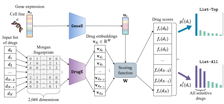
Figure 1. Overall Framework. The cell line embeddings $\mbox{$\mathbf{u}$}_{c}$ and drug embeddings $\mbox{$\mathbf{v}$}_{d_{i}}$ are used to score the drugs $d_{i}\in\mbox{$\mathcal{D}$}_{c}$. Each ranking method utilizes a different ranking objective and thus utilizes the scores $f_{c}(d_{i})$ differently. The pretrained encoder $\mathop{\mathtt{GeneE}}\limits$ is finetuned during ranking optimization.

In order to select and prioritize sensitive drugs in each cell line, our proposed LeToR methods optimize different objectives that inducing the correct ranking structure among the top-sensitive or all involved drugs in each cell line. Figure 1 presents an overall scheme of our proposed methods. To induce the correct ranking structure, each method learns to accurately score drugs in each cell line using the learned cell line and drug embeddings. The embeddings and scoring function are learned in a fully data-driven manner from the drug response data. Intuitively, the cell line latent space embeds the genomic and response information of cell lines, while the drug latent space embeds the structural and sensitivity information for drugs. The cell line embeddings are initially learned from the gene expression profiles using a pre-trained auto-encoder model $\mathop{\mathtt{GeneAE}}\limits$ (Section 3.2). The drug embeddings are learned from the molecular fingerprints (Section 3.3). During training, the cell line and drug embeddings are then used and updated to correctly score drugs against each cell line using a learnable scoring function (Section 3.4.1). Note that $\mathop{\mathtt{List\text{-}One}}\limits$ and $\mathop{\mathtt{List\text{-}All}}\limits$ utilize the same scoring function, however, optimize separate ranking objectives.

3.2. Pretraining for Cell Line Embeddings

Figure 2. Pretraining framework. Given a gene expression $\mathbf{x}_{c}$, $\mathop{\mathtt{GeneAE}}\limits$ reconstructs it as $\widetilde{\mathbf{x}}_{c}$ through the auto-encoder, meanwhile learning an embedding $\mbox{$\mathbf{u}$}_{c}$ in the latent space.

In order to learn rich informative cell line embeddings, we pretrain a stacked auto-encoder framework $\mathop{\mathtt{GeneAE}}\limits$, similar to existing gene expression auto-encoder frameworks(Xie et al., 2017; Dincer et al., 2020). Figure 2 presents the architecture of $\mathop{\mathtt{GeneAE}}\limits$. $\mathop{\mathtt{GeneAE}}\limits$ embeds the rich genomic information into a latent space, and learns the complex and non-linear interactions among genes. Specifically, $\mathop{\mathtt{GeneAE}}\limits$ leverages the gene expression profile $\mathbf{x}_{c}$ to learn a low-dimensional embedding $\mbox{$\mathbf{u}$}_{c}$ via the encoder $\mathop{\mathtt{GeneE}}\limits$, followed by reconstruction of the expression profile from $\mbox{$\mathbf{u}$}_{c}$ via the decoder $\mathop{\mathtt{GeneD}}\limits$. These embeddings out of the pretrained $\mathop{\mathtt{GeneE}}\limits$ are used to score drugs in each cell line during the downstream ranking (Section 3.4.1). Such embeddings can be utilized as transferable representations of cell lines that can potentially enable better generalizability of downstream drug scoring/ranking models. In summary, these embeddings can potentially improve the performance of drug ranking models by leveraging the shared biological features across cell lines.

As any other pretraining module(Erhan et al., 2010), $\mathop{\mathtt{GeneAE}}\limits$ has two training stages: pretraining, and finetuning. During pretraining, the model parameters are learned via back-propagation by minimizing the reconstruction error (here, MSE) from the actual and reconstructed gene expression data as,

(1) $$\min\nolimits_{\theta_{\textsc{\mbox{$\mathop{\mathtt{GeneE}}\limits$}}},\theta_{\textsc{\mbox{$\mathop{\mathtt{GeneD}}\limits$}}}}\frac{1}{|\mbox{$\mathcal{C}$}|}\sum_{c\in\mbox{$\mathcal{C}$}}||\mathbf{x}_{c}-\widetilde{\mathbf{x}}_{c}||_{2}^{2},$$

where $\mathbf{x}_{c}$ denotes the input gene expression of cell line $c$, $\widetilde{\mathbf{x}}_{c}=\mbox{$\mathop{\mathtt{GeneD}}\limits$}(\mbox{$\mathop{\mathtt{GeneE}}\limits$}(\mathbf{x}_{c}))$ denotes the corresponding reconstructed gene expression, $\theta_{\textsc{\mbox{$\mathop{\mathtt{GeneE}}\limits$}}}$ and $\theta_{\textsc{\mbox{$\mathop{\mathtt{GeneD}}\limits$}}}$ denote the learnable parameters of $\mathop{\mathtt{GeneE}}\limits$ and $\mathop{\mathtt{GeneD}}\limits$, respectively, and $\mathcal{C}$ denotes the set of input cell lines. During pretraining, parameters of both $\mathop{\mathtt{GeneE}}\limits$ and $\mathop{\mathtt{GeneD}}\limits$ modules are learned, and the learned parameters of $\mathop{\mathtt{GeneE}}\limits$ are transferred and finetuned during the optimization for downstream ranking tasks. The finetuning of pretrained $\mathop{\mathtt{GeneE}}\limits$ adapts the output embeddings toward the specific downstream ranking.

3.3. Embedding Drugs from Fingerprints

In this work, molecular fingerprints(Rogers and Hahn, 2010) are leveraged to learn informative drug embeddings via a low-dimensional projection. These fingerprints are discrete feature vectors representing the presence of molecular substructures in a drug given a fixed vocabulary. Typically, such fingerprints need to be high-dimensional to sufficiently capture all relevant structural information. On the other hand, the drug embeddings can selectively encode relevant structural information (specific to the ranking task) as non-linear functions of input fingerprints. These embeddings are further used to score drugs in each cell line, and are learned during ranking optimization given drug response data across multiple cell lines. Such learned embeddings enable accurate drug scoring since similar drugs in terms of structures and sensitivities across multiple cell lines obtain similar embeddings. To learn such embeddings of dimension $M$ ($M$ is a hyperparameter), we used a fully connected neural network $\mathop{\mathtt{DrugE}}\limits$. As inputs to $\mathop{\mathtt{DrugE}}\limits$, we used Morgan count fingerprints(Rogers and Hahn, 2010) with radius = 3 and 2,048 bits. While graph neural networks (GNNs)(Wu et al., 2021) have demonstrated promising empirical performance in molecular prediction tasks(Zhang et al., 2022), we observed inferior ranking performance from the drug embeddings learned from GNNs compared to those learned from fingerprints, from preliminary experiments. This is possibly due to the limited number of unique drugs in our datasets.

3.4. Listwise Ranking for Top-One Drug: $\mathop{\mathtt{List\text{-}One}}\limits$

We adopted the standard ListNet(Cao et al., 2007) objective to develop a neural listwise ranking method, $\mathop{\mathtt{List\text{-}One}}\limits$. $\mathop{\mathtt{List\text{-}One}}\limits$ considers the entire ranking structure at a time and focuses on accurately estimating the top-one probability of drugs. The top-one probability of a drug $d$, denoted as $p_{c}(d)$, is its probability of being ranked at the top given the scores of all involved drugs in the cell line $c$. Formally, the predicted top-one probability denoted as $p_{c}^{f}(d)$ is defined as follows:

(2) $$p_{c}^{f}(d)=\frac{\exp{(f_{c}(d))}}{\sum_{d_{j}\in\mbox{$\mathcal{D}$}_{c}}\exp{(f_{c}(d))}},$$

where $f_{c}(d)$ denotes the score of drug $d$ in cell line $c$ (which will be discussed later in Section 3.4.1). The top-one probabilities are optimized using the cross-entropy loss as follows:

(3) $$\min_{\Theta}-\sum_{c\in\mbox{$\mathcal{C}$}}\left[\sum_{d\in\mbox{$\mathcal{D}$}_{c}}p_{c}^{top}(d)\log(p_{c}^{f}(d))\right],$$

where $\Theta$ denotes the learnable parameters in the model; and $p_{c}^{top}(d)$ denotes the ground-truth top-one probability of drug $d$ in the cell line $c$ according to the ground-truth drug responses. In this study, the drug responses are quantified with Area Under the dose-response Curve denoted as AUC, where smaller AUC values indicate higher drug sensitivities. $p_{c}^{top}(d)$ is computed via Equation 2 by replacing $f_{c}(d)$ with the negated AUCs (since lower AUCs indicate higher drug sensitivities). Minimizing the above loss reduces the discrepancy between the predicted and the ground-truth top-one probability distribution over drugs in each cell line. This results in an accurate estimation of the top-one probability, which enables an accurate selection of the most sensitive drug in each cell line. During the optimization, $\mathop{\mathtt{List\text{-}One}}\limits$ (and $\mathop{\mathtt{List\text{-}All}}\limits$ presented in the following section similarly) finetunes $\mathop{\mathtt{GeneE}}\limits$ (Section 3.2) and learns $\mathop{\mathtt{DrugE}}\limits$ (Section 3.3). This enables the cell line and drug embeddings out of $\mathop{\mathtt{GeneE}}\limits$ and $\mathop{\mathtt{DrugE}}\limits$, respectively, to encode task-relevant information.

3.4.1. Drug Scoring

In order to score the drug $d$ in a cell line $c$, we used a parameterized bilinear function denoted as $f_{c}(d)$. The function $f_{c}(d)$ is parameterized via a learnable weight matrix $\mathbf{W}\in\mathbb{R}^{|\mbox{$\mathbf{u}$}_{c}|\times|\mbox{$\mathbf{v}$}_{d}|}$, and is applied over the $\mbox{$\mathbf{u}$}_{c}\in\mathbb{R}^{|\mbox{$\mathbf{u}$}_{c}|}$ and $\mbox{$\mathbf{v}$}_{d}\in\mathbb{R}^{|\mbox{$\mathbf{v}$}_{d}|}$ as follows:

(4) $$f_{c}(d)=\mbox{$\mathbf{u}$}_{c}^{\intercal}\mathbf{W}\mbox{$\mathbf{v}$}_{d},$$

where, $\mathbf{W}$ is learned via backpropagation in an end-to-end manner during optimization. Intuitively, the learnable full-rank weight matrix $\mathbf{W}$ in the bilinear scoring function can capture complex and relevant interactions between the two latent vectors. Once the scores for all drugs in a cell line $c$ (i.e., $\mbox{$\mathcal{D}$}_{c}$) are obtained, the drugs $\mbox{$\mathcal{D}$}_{c}$ are sorted based on such scores in descending order. The most sensitive drugs in $c$ will have higher scores than the insensitive ones in $c$. Note that ranking-based methods such as our proposed ones will achieve optimal ranking performance as long as these scores induce correct ranking structure; the scores do not need to be exactly identical to the drug response scores (i.e., AUC values).

3.5. Listwise Ranking for All Sensitive Drugs: $\mathop{\mathtt{List\text{-}All}}\limits$

Since $\mathop{\mathtt{List\text{-}One}}\limits$ focuses solely on the top-ranked drug, it may lead to suboptimal performance in terms of selecting all the sensitive drugs in each cell line, as demonstrated in our experiments (Section 5.1), To address this, we proposed a new listwise neural ranking method, $\mathop{\mathtt{List\text{-}All}}\limits$ with an objective that can optimize the selection of all sensitive drugs in each cell line. $\mathop{\mathtt{List\text{-}All}}\limits$ leverages the entire ranking structure at a time and follows a similar architecture to $\mathop{\mathtt{List\text{-}One}}\limits$. But unlike $\mathop{\mathtt{List\text{-}One}}\limits$, $\mathop{\mathtt{List\text{-}All}}\limits$ estimates the probability of a drug being sensitive given the scores of all drugs, where higher scores induce higher probabilities. Since the estimated probability of each drug being sensitive is dependent on the scores of all other drugs in the list, $\mathop{\mathtt{List\text{-}All}}\limits$ is a listwise ranking method. $\mathop{\mathtt{List\text{-}All}}\limits$ aims to minimize the distance between such estimated score-induced probabilities and the ground-truth sensitivity labels across all drugs in each cell line. Specifically, $\mathop{\mathtt{List\text{-}All}}\limits$ is trained by minimizing the following loss:

(5) $$\min_{\Theta}-\sum_{c\in\mbox{$\mathcal{C}$}}\left[\sum_{d\in\mbox{$\mathcal{D}$}_{c}}l_{c}(d)\log(s_{c}^{f}(d))\right],$$

where $\Theta$ denotes the learnable parameters in the model; $l_{c}(d)$ is a binary sensitivity label indicating whether drug $d$ is sensitive in cell line $c$; and $s_{c}^{f}(d)$ denotes the probability of drug $d$ to be sensitive in the cell line $c$. Formally, $s_{c}^{f}(d)$ is computed from the predicted scores via the parameterized softmax as:

(6) $$s_{c}^{f}(d)=\frac{\exp{(f_{c}(d)/\tau)}}{\sum_{d_{j}\in\mbox{$\mathcal{D}$}_{c}}\exp{(f_{c}(d)/\tau)}},$$

where $\tau$ is the temperature (a scaling factor > 0) that controls the softness/sharpness of the score-induced probability distribution while maintaining the relative ranks. A lower scaling factor results in a sharper probability distribution with higher probabilities on very few drugs. Note that the scaling factor can also be applied similarly in Equation 2, however, we observed no notable performance difference empirically. For $\mathop{\mathtt{List\text{-}All}}\limits$, we fix $\tau$ to 0.5. Note that the optimization objective (Equation 5) resembles the ListNet objective (Equation 3) in the sense that both aim to minimize the cross-entropy between two score-induced empirical probability distributions.

4. Materials

In this section, we present the data sets and baselines used in Sections 4.1 and 4.2, respectively; the experimental setting in Section 4.3; and the evaluation metrics adopted to evaluate ranking performance in Section 4.4.

4.1. Dataset

Table 2. Dataset Overview

Dataset	|$\mathcal{C}$ |	|$\mathcal{D}$ |	#AUCs	#d/$\mathcal{C}$	c/$\mathcal{D}$	m%
CTRP	809	545	357,544	442	656	18.9

• In this table, the columns $|\mbox{$\mathcal{C}$}|$, $|\mbox{$\mathcal{D}$}|$, and #AUCs denote the number of unique cell lines, drugs and cell-line drug response pairs, respectively. The columns #d/$\mathcal{C}$, c/$\mathcal{D}$ and m% denote the average number of drugs per cell line, average number of cell lines per drug, and the missing percentage of responses, respectively.

We collected the drug response data set from the Cancer Therapeutic Response Portal version 2 (CTRP)(Seashore-Ludlow et al., 2015). We focused on this data set because it covers a large number of cell lines and drugs compared to other available data sets. We utilized the Cancer Cell Line Encyclopedia version 22Q1 (CCLE)(Barretina et al., 2012) for the gene expression data. CCLE provides multi-omics data (genomic, transcriptomic and epigenomic) for more than 1,000 cancer cell lines. However, in this study, we only used the gene expression (transcriptomic) data following (He et al., 2020). The drug responses are measured using AUC sensitivity scores, with lower AUC indicating higher sensitivity of a drug in a cell line. For the drugs with missing responses in a cell line, the corresponding drug-cell line pairs were not included in the training of models. For the cell lines that could not be mapped to CCLE, those cell lines and their associated drug responses were excluded from our experiments. Since CTRP has more cell lines than other available datasets in the literature, it is an appropriate choice for evaluating computational methods in drug selection for new cell lines, which is the primary focus of this work. This work is motivated based on the belief that such a setup is more relevant to real-life scenarios where the goal is to suggest potential anti-cancer drugs for new patients.

4.2. Baselines

We use two strong baseline methods: $\mathop{\mathtt{pLETORg}}\limits$ (He et al., 2020) and $\mathop{\mathtt{DeepCDR}}\limits$ (Liu et al., 2020). Unlike our proposed methods, $\mathop{\mathtt{pLETORg}}\limits$ is a pairwise ranking approach that learns the drug and cell line embeddings by explicitly pushing sensitive drugs to the top of the ranking list and by further optimizing the ranking structure among the sensitives. Unlike $\mathop{\mathtt{pLETORg}}\limits$, our proposed methods leverage drug structural and gene expression information to learn more informative embeddings that may enable improved ranking performance. Additionally, different from $\mathop{\mathtt{pLETORg}}\limits$, our proposed methods utilize a learnable scoring function to capture the complex interactions between embeddings. While $\mathop{\mathtt{pLETORg}}\limits$ explicitly enforces similarity regularization on cell line embeddings using the gene expression-based similarity of cell lines, our methods enforce such genomic similarity by embedding cell lines in the latent space via the pretrained $\mathop{\mathtt{GeneE}}\limits$. Different from our proposed methods and the baseline $\mathop{\mathtt{pLETORg}}\limits$, $\mathop{\mathtt{DeepCDR}}\limits$, one of the state-of-the-art regression models for anti-cancer drug response prediction, learns to estimate the exact response scores of every drug in each cell line.

4.3. Experimental Setting

According to the setting of He et al. (He et al., 2020), a percentile labeling scheme was used to label drugs as sensitive or insensitive. The sensitivity threshold for each cell line was determined as the top-5 percentile of its drug responses. In order to assess the ranking performance on new cell lines, we employed a leave-cell-lines-out (LCO) validation setting such that this setting resembles the real-world scenario when known drugs are investigated for their sensitivity or anti-cancer potential in new patients. We randomly split all the cell lines from each cancer type into five folds. In each run, we used the four folds from each cancer type for training and the other fold for testing. We use the cell lines from all the cancer types for 4 folds and their corresponding drug response data collectively for training. We use the cell lines in the other left-out fold as new (unseen) cell lines for model testing. This process was repeated five times with each fold serving as the test fold exactly once. For $\mathop{\mathtt{pLETORg}}\limits$, we follow the ‘leave-one-out’ setup(He et al., 2020) in that the cell line embeddings were learned only for the training cell lines, and the embeddings for the test cell lines were interpolated from the nearest neighboring training cell lines in the latent space. For our proposed methods, we use the gene expression profiles of only the training cell lines to pretrain $\mathop{\mathtt{GeneAE}}\limits$.

4.4. Evaluation Metrics

In order to evaluate the ranking performance, we generated the true ranking list using the ground-truth AUC response values and the predicted ranking list using the estimated scores out of the models. We then compared the two ranking lists (or a portion of them) using popular evaluation metrics: average precision at $K$ ($\mathop{\mathtt{AP}}\limits$@K), and average hit at $K$ ($\mathop{\mathtt{AH}}\limits$@K), which are commonly used in Information Retrieval systems. Higher $\mathop{\mathtt{AP}}\limits$@K and $\mathop{\mathtt{AH}}\limits$@K indicate better drug selection where the top-ranked drugs in the predicted ranking list are sensitive. In addition to $\mathop{\mathtt{AP}}\limits$ and $\mathop{\mathtt{AH}}\limits$, concordance index ($\mathop{\mathtt{CI}}\limits$) and concordance index among the sensitive drugs ($\mathop{\mathtt{sCI}}\limits$) (He et al., 2020) are also used to evaluate the overall quality of the predicted ranking structure among all drugs and sensitive drugs, respectively. Note that high $\mathop{\mathtt{CI}}\limits$ and $\mathop{\mathtt{sCI}}\limits$ values do not necessarily result in high $\mathop{\mathtt{AP}}\limits$ or $\mathop{\mathtt{AH}}\limits$ since the ranking structure can be well preserved without pushing the few sensitive drugs (which constitutes only 5% of the total drugs) to the very top. On the other hand, high $\mathop{\mathtt{AP}}\limits$/$\mathop{\mathtt{AH}}\limits$ indicates the most sensitive drugs are ranked at the top, but this does not necessarily result in high $\mathop{\mathtt{CI}}\limits$/$\mathop{\mathtt{sCI}}\limits$. In this work, since we primarily focus on identifying the top-$k$ most sensitive drugs in each cell line, we prioritize and emphasize the $\mathop{\mathtt{AP}}\limits$ and $\mathop{\mathtt{AH}}\limits$ metrics over the $\mathop{\mathtt{sCI}}\limits$ and $\mathop{\mathtt{CI}}\limits$ metrics when evaluating and interpreting our results.

5. Results

5.1. Overall Comparison

Table 3. Overall Comparison for CTRP in LCO validation

model	AP@1	AP@3	AH@3	AP@5	AH@5	AP@10	AH@10	AP@20	AH@20	AP@40	AH@40	AP@60	AH@60
$\mathop{\mathtt{pLETORg}}\limits$	0.9308*	0.9586	2.6853	0.9391	4.2454	0.8962	7.3525	0.8178	11.9248	0.7286	17.1087	0.6877	19.5646
$\mathop{\mathtt{pLETORg}}\limits$	0.9306	0.9598*	2.6944	0.9402	4.2756	0.9018	7.4802	0.8255	12.0889	0.7361	17.3179	0.7011	19.3712
$\mathop{\mathtt{pLETORg}}\limits$	0.9306	0.9596	2.6968*	0.9402	4.2731	0.9018	7.4716	0.8250	12.0936	0.7351	17.3506*	0.7002	19.4150
$\mathop{\mathtt{pLETORg}}\limits$	0.9306	0.9593	2.6951	0.9410*	4.2582	0.8999	7.3960	0.8222	12.0270	0.7328	17.2086	0.6951	19.4621
$\mathop{\mathtt{pLETORg}}\limits$	0.9306	0.9597	2.6943	0.9402	4.2829*	0.9023	7.4804*	0.8257*	12.0962*	0.7364*	17.3279	0.7023*	19.3091
$\mathop{\mathtt{pLETORg}}\limits$	0.9306	0.9595	2.6878	0.9395	4.2791	0.9026*	7.4467	0.8246	12.0456	0.7353	17.2695	0.6995	19.3624
$\mathop{\mathtt{pLETORg}}\limits$	0.9306	0.9587	2.6748	0.9376	4.2236	0.8988	7.3600	0.8192	12.0065	0.7304	17.2451	0.6893	19.7447*
$\mathop{\mathtt{DeepCDR}}\limits$	0.9260*	0.9296*	2.4716	0.9015	4.0904	0.8646	7.4440*	0.8025	11.5779	0.7155	16.7472*	0.6736	19.3054*
$\mathop{\mathtt{DeepCDR}}\limits$	0.9129	0.9271	2.5151*	0.9035	4.1096*	0.8665*	7.4384	0.8036*	11.7047*	0.7211*	16.7447	0.6791*	19.3008
$\mathop{\mathtt{DeepCDR}}\limits$	0.9209	0.9282	2.5087	0.9064*	4.0324	0.8599	7.3529	0.7984	11.5311	0.7118	16.5821	0.6700	19.2082
$\mathop{\mathtt{List\text{-}One}}\limits$	0.9478*	0.9523*	2.5284	0.9170	3.9832	0.8614	7.2736	0.7929	12.0092	0.7152	17.4724	0.6773	20.0047
$\mathop{\mathtt{List\text{-}One}}\limits$	0.9359	0.9499	2.6392*	0.9278	4.1952*	0.8830	7.4661	0.8128	12.3445	0.7344	17.6828	0.6963	20.1293
$\mathop{\mathtt{List\text{-}One}}\limits$	0.9423	0.9507	2.6285	0.9293*	4.1583	0.8833*	7.4334	0.8115	12.1450	0.7304	17.5116	0.6902	20.0350
$\mathop{\mathtt{List\text{-}One}}\limits$	0.9393	0.9485	2.6315	0.9269	4.1909	0.8828	7.5999*	0.8174*	12.4297	0.7389*	17.9255	0.7024*	20.2904
$\mathop{\mathtt{List\text{-}One}}\limits$	0.9165	0.9371	2.5749	0.9152	4.1013	0.8694	7.5055	0.8065	12.5335*	0.7330	17.8804	0.6970	20.2376
$\mathop{\mathtt{List\text{-}One}}\limits$	0.9030	0.9300	2.5543	0.9106	4.0587	0.8640	7.4101	0.8009	12.4205	0.7262	17.9959*	0.6924	20.3382*
$\mathop{\mathtt{List\text{-}All}}\limits$	0.9480*	0.9610*	2.6985	0.9420	4.2885	0.9087	7.6208	0.8333	12.1992	0.7429	17.4686	0.7012	20.0028
$\mathop{\mathtt{List\text{-}All}}\limits$	0.9295	0.9537	2.7142*	0.9403	4.3000	0.9060	7.6104	0.8327	12.2481	0.7442	17.5094	0.7035	19.9869
$\mathop{\mathtt{List\text{-}All}}\limits$	0.9421	0.9597	2.6984	0.9442*	4.2919	0.9094	7.6224	0.8345	12.1688	0.7436	17.4484	0.7020	19.9981
$\mathop{\mathtt{List\text{-}All}}\limits$	0.9365	0.9604	2.6934	0.9411	4.3119*	0.9067	7.6108	0.8334	12.1745	0.7429	17.4458	0.7014	19.9993
$\mathop{\mathtt{List\text{-}All}}\limits$	0.9395	0.9581	2.7076	0.9414	4.3056	0.9102*	7.6232	0.8339	12.1874	0.7432	17.4571	0.7020	19.9871
$\mathop{\mathtt{List\text{-}All}}\limits$	0.9255	0.9452	2.6474	0.9255	4.2547	0.8890	7.7577*	0.8276	12.6216	0.7489	17.9918	0.7116	20.3199
$\mathop{\mathtt{List\text{-}All}}\limits$	0.9418	0.9598	2.6903	0.9409	4.3037	0.9067	7.6969	0.8361*	12.3357	0.7478	17.6577	0.7073	20.0894
$\mathop{\mathtt{List\text{-}All}}\limits$	0.8586	0.9120	2.5588	0.8989	4.1607	0.8678	7.6558	0.8130	12.7728*†	0.7412	18.2956	0.7084	20.4696
$\mathop{\mathtt{List\text{-}All}}\limits$	0.9188	0.9417	2.6518	0.9268	4.2490	0.8901	7.7238	0.8274	12.6474	0.7497*	17.9691	0.7117*	20.3631
$\mathop{\mathtt{List\text{-}All}}\limits$	0.8147	0.8828	2.4717	0.8734	4.0153	0.8461	7.5360	0.7965	12.7146	0.7291	18.3331*†	0.6980	20.5291*†

• The performances of the best performing model are in bold. * indicates the best observed performance in a metric for a given model. $\dagger$ indicates that the model performs significantly better compared to $\mathop{\mathtt{pLETORg}}\limits$ according to a Wilcoxon signed rank test with Bonferroni correction at 5% significance level.

Table 3 shows that, overall, $\mathop{\mathtt{List\text{-}All}}\limits$ consistently outperforms all other methods in most metrics. Specifically, $\mathop{\mathtt{List\text{-}All}}\limits$ achieved the best $\mbox{$\mathop{\mathtt{AH}}\limits$}@K$ scores with impressive results of 2.7142, 4.3119, 7.7577, 12.7728, and 18.3331 for $K=$ 3, 5, 10, 20, and 40, respectively. Following $\mathop{\mathtt{List\text{-}All}}\limits$, the other listwise ranking method, $\mathop{\mathtt{List\text{-}One}}\limits$ achieved the second-best performance in terms of $\mbox{$\mathop{\mathtt{AH}}\limits$}@K$. Overall, $\mathop{\mathtt{List\text{-}All}}\limits$ achieved better $\mathop{\mathtt{AH}}\limits$@10, $\mathop{\mathtt{AH}}\limits$@20 and $\mathop{\mathtt{AH}}\limits$@40 over $\mathop{\mathtt{List\text{-}One}}\limits$, whereas both methods achieved competitive hit rates up to $K\leq 5$. This suggests that $\mathop{\mathtt{List\text{-}All}}\limits$ is particularly effective in pushing almost all sensitive drugs to the top while $\mathop{\mathtt{List\text{-}One}}\limits$ was able to push only a few most sensitive drugs. This is further reflected in the consistent improvements observed in $\mathop{\mathtt{AH}}\limits$ and $\mathop{\mathtt{AP}}\limits$. Compared to $\mathop{\mathtt{List\text{-}One}}\limits$, $\mathop{\mathtt{List\text{-}All}}\limits$ improved $\mathop{\mathtt{H}}\limits$@10, $\mathop{\mathtt{H}}\limits$@20, and $\mathop{\mathtt{H}}\limits$@40 for 33.9% (55), 44.6% (72) and 39.5% (64) of 162 new cell lines by 3.8%, 3.0% and 1.4%, respectively. Such superior performance of $\mathop{\mathtt{List\text{-}All}}\limits$ over $\mathop{\mathtt{List\text{-}One}}\limits$ can be attributed to the ability of $\mathop{\mathtt{List\text{-}All}}\limits$ to accurately estimate the probability of drugs being sensitive in each cell line while $\mathop{\mathtt{List\text{-}One}}\limits$ focuses solely on the most sensitive (i.e., top-ranked) drug while ignoring the other sensitive drugs.

Furthermore, $\mathop{\mathtt{List\text{-}All}}\limits$ outperformed the best baseline method, $\mathop{\mathtt{pLETORg}}\limits$, across all metrics. Moreover, compared to $\mathop{\mathtt{pLETORg}}\limits$, both $\mathop{\mathtt{List\text{-}All}}\limits$ and $\mathop{\mathtt{List\text{-}One}}\limits$ demonstrated significantly better or competitive performance in $\mathop{\mathtt{AH}}\limits$ and $\mathop{\mathtt{AP}}\limits$. This implies that all our proposed methods can improve the ranking performance over $\mathop{\mathtt{pLETORg}}\limits$ by explicitly leveraging auxiliary information such as gene expression profiles and molecular fingerprints. Specifically, compared to $\mathop{\mathtt{pLETORg}}\limits$, the best-performing method, $\mathop{\mathtt{List\text{-}All}}\limits$, demonstrated statistically significant improvement in $\mathop{\mathtt{H}}\limits$@20, $\mathop{\mathtt{H}}\limits$@40 and $\mathop{\mathtt{H}}\limits$@60 for 50.6% (82), 53.0% (86) and 45.7% (74) of 162 new cell lines by 8.6%, 6.3% and 5.0%, respectively, while achieving marginally better hit rates for $K<20$. Additionally, $\mathop{\mathtt{List\text{-}All}}\limits$ achieved better $\mathop{\mathtt{AP}}\limits$@20 and $\mathop{\mathtt{AP}}\limits$@40 than $\mathop{\mathtt{pLETORg}}\limits$, improving $\mathop{\mathtt{P}}\limits$@20 and $\mathop{\mathtt{P}}\limits$@40 for 53.7% (87) and 58.0% (94) of 162 new cell lines by 1.1% and 3.0% on average, respectively. Such consistent and significant improvement across multiple $\mathop{\mathtt{AH}}\limits$ and $\mathop{\mathtt{AP}}\limits$ metrics on a large percentage of cell lines provides strong evidence that $\mathop{\mathtt{List\text{-}All}}\limits$ clearly outperforms the best baseline method $\mathop{\mathtt{pLETORg}}\limits$ in drug selection and prioritization.

These results suggest that $\mathop{\mathtt{List\text{-}All}}\limits$ can effectively leverage the drug structure information and the entire ranking structure to learn richer latent representations while focusing on learning to select all the sensitive drugs in a cell line. The consistent sub-par performance of $\mathop{\mathtt{pLETORg}}\limits$ compared to $\mathop{\mathtt{List\text{-}All}}\limits$ could be due to the fact that $\mathop{\mathtt{pLETORg}}\limits$ only focuses on the pairwise relative ordering without considering the overall ranking structure. Since there are significantly more insensitive drugs than sensitive ones in each cell line, such pairwise methods may struggle to preserve the ordering between pairs of sensitive and insensitive drugs, thereby leading to a sub-optimal selection of all sensitive drugs. Overall, all ranking-based methods outperformed the state-of-the-art regression model, $\mathop{\mathtt{DeepCDR}}\limits$, across all metrics. This indicates that learning to estimate the exact drug responses while obtaining a lower overall MSE does not necessarily guarantee accurate score estimation for the sensitive drugs, which constitutes only 5% of all drugs in a cell line. This leads to sub-par performance of $\mathop{\mathtt{DeepCDR}}\limits$ in terms of selecting and prioritizing the most sensitive drugs in a cell line.

5.2. Study of Cell Line embeddings

We evaluated the quality of cell line embeddings based on their ability to capture the drug response profiles. In order to quantitatively evaluate this, we computed the pairwise similarities of cell lines in two different ways: 1) using the radial basis function (RBF) kernel on the learned cell line embeddings out of the best baseline, $\mathop{\mathtt{pLETORg}}\limits$, and the best method, $\mathop{\mathtt{List\text{-}All}}\limits$, denoted as $\mathop{\mathtt{sim_{c}\text{-}{B}}}\limits$ and $\mathop{\mathtt{sim_{c}\text{-}{M}}}\limits$, respectively; and 2) using Spearman rank correlation on the ranked lists of drugs given their drug response profiles, denoted as $\mathop{\mathtt{sim_{c}\text{-}{R}}}\limits$. Intuitively, $\mathop{\mathtt{sim_{c}\text{-}{B}}}\limits$ and $\mathop{\mathtt{sim_{c}\text{-}{M}}}\limits$ are higher for pairs of cell lines that are close in their corresponding latent spaces. Meanwhile, $\mathop{\mathtt{sim_{c}\text{-}{R}}}\limits$ is higher for pairs of cell lines if they share similar drug response profiles. Note that since every drug may not have recorded responses in each cell line, $\mathop{\mathtt{sim_{c}\text{-}{R}}}\limits$ for a pair of cell lines $p$ and $q$ is computed from drug response data of the shared set of drugs, $\mbox{$\mathcal{D}$}_{p}\cap\mbox{$\mathcal{D}$}_{q}$, whose responses are recorded for both cell lines.

We hypothesize that the latent space captures the ranking structures across drugs, implying that the cell lines close in the latent space have similar drug response profiles (i.e., $\mathop{\mathtt{sim_{c}\text{-}{B}}}\limits$ and $\mathop{\mathtt{sim_{c}\text{-}{M}}}\limits$ are well correlated with $\mathop{\mathtt{sim_{c}\text{-}{R}}}\limits$). In order to validate our hypothesis, we calculated the Pearson correlations between $\mathop{\mathtt{sim_{c}\text{-}{B}}}\limits$ and $\mathop{\mathtt{sim_{c}\text{-}{R}}}\limits$, denoted as $\mathtt{corr_{c}(B,R)}$, and between $\mathop{\mathtt{sim_{c}\text{-}{M}}}\limits$ and $\mathop{\mathtt{sim_{c}\text{-}{R}}}\limits$, denoted as $\mathtt{corr_{c}(M,R)}$. We observed that the pairwise cell line similarities induced by their drug response profiles are better correlated with the similarities induced in the latent space learned by $\mathop{\mathtt{List\text{-}All}}\limits$ compared to $\mathop{\mathtt{pLETORg}}\limits$ (Pearson correlations $\mathtt{corr_{c}(M,R)}$ vs. $\mathtt{corr_{c}(B,R)}$: 0.162 vs. 0.151). This suggests that $\mathop{\mathtt{List\text{-}All}}\limits$ learns informative cell line embeddings that can capture the overall ranking structure more effectively than $\mathop{\mathtt{pLETORg}}\limits$. Intuitively, $\mathop{\mathtt{List\text{-}All}}\limits$ may benefit from the fact that it uses the gene expression profile to learn cell line embeddings; and because cell lines with similar gene expression profiles typically demonstrate similar drug response profiles. Although $\mathop{\mathtt{pLETORg}}\limits$ uses a weighted regularizer to constrain cell line embeddings based on their genomic similarity it may not fully capture the complex relationships between the gene expressions of two cell lines. Explicitly learning embeddings from gene expressions allows $\mathop{\mathtt{List\text{-}All}}\limits$ to extract more nuanced task-relevant relationships and a desired notion of similarity between cell lines.

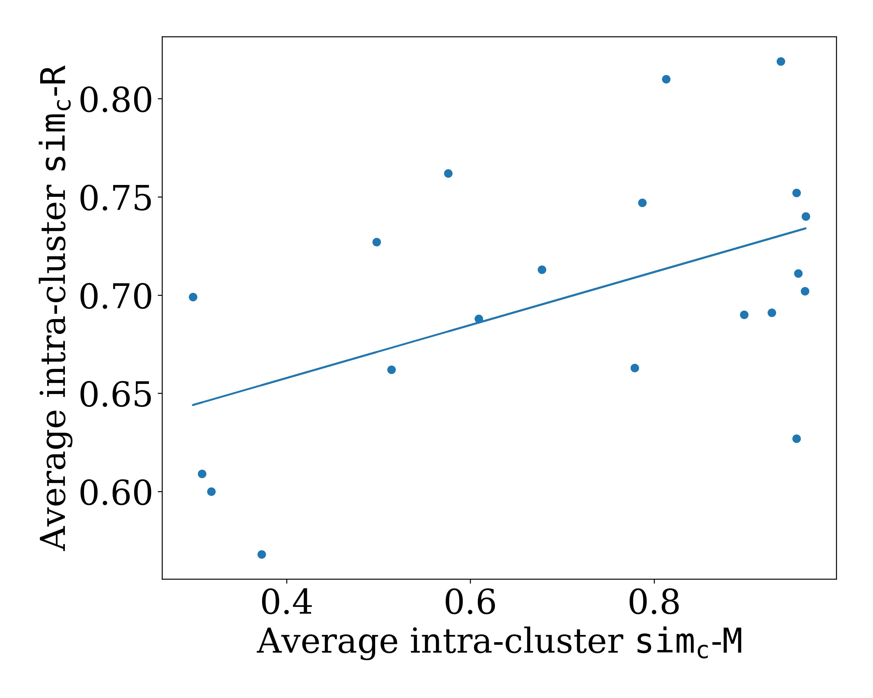
Figure 3. Scatter plot of intra-cluster similarities, computed as the average of $\mathop{\mathtt{sim_{c}\text{-}{R}}}\limits$ and $\mathop{\mathtt{sim_{c}\text{-}{M}}}\limits$ within each cluster.

We further evaluated the quality of their latent spaces in more detail with respect to clustering compactness and different cancer types. We applied a 20-way clustering using CLUTO(Karypis, 2002) on the embeddings. Figure 3 presents the intra-cluster similarities, i.e., $\mathop{\mathtt{sim_{c}\text{-}{R}}}\limits$ vs. $\mathop{\mathtt{sim_{c}\text{-}{M}}}\limits$ averaged across cell lines in each cluster. We observed that compact clusters in the latent space contained cell lines with more similar drug-ranking structures. This is evident from the fitted line with a positive slope as shown in Figure 3. This further supports our hypothesis that the cell line latent space learned by $\mathop{\mathtt{List\text{-}All}}\limits$ effectively captures the drug response profiles. Moreover, our clustering analysis can uncover unobvious or previously unknown similarities among cell lines from different cancer types, which may not be apparent from the observed drug response data.

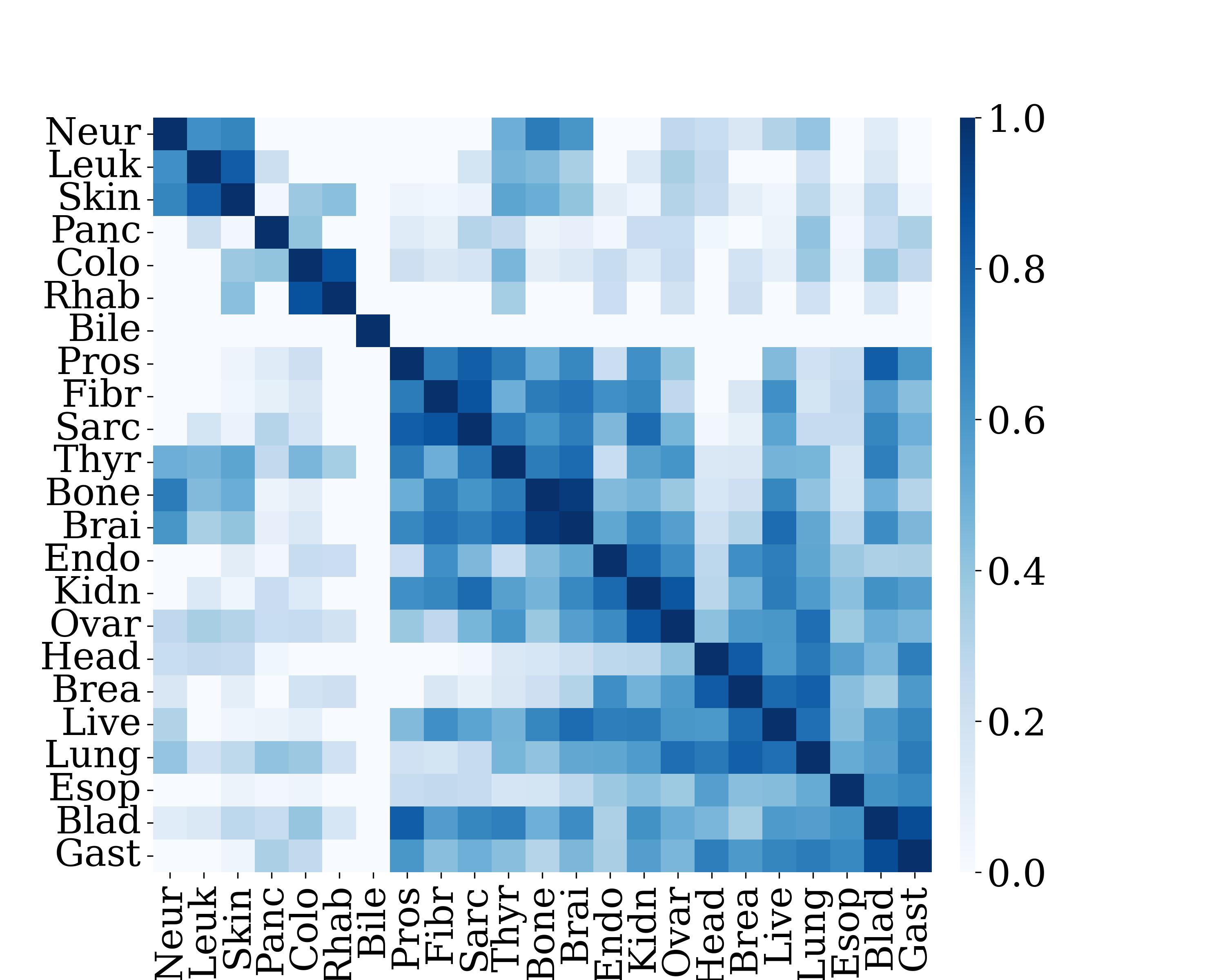
(a) Based on the distribution
of cell lines across clusters.

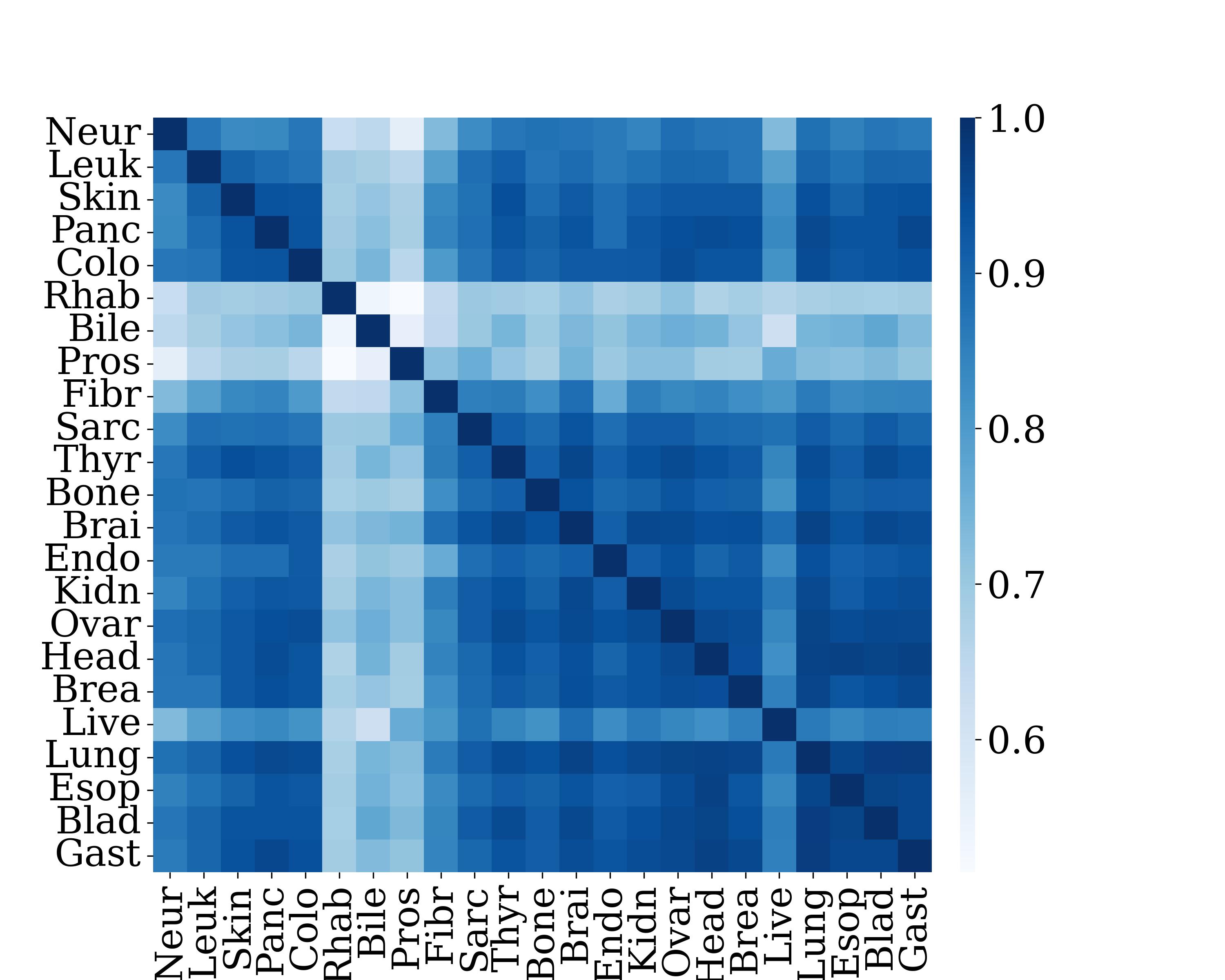
(b) Based on average $\mathop{\mathtt{sim_{c}\text{-}{R}}}\limits$
among cell lines

Figure 4. Comparison of two pairwise similarity matrices across different cancer types.

Figure 4a presents the average pairwise similarities with respect to clustering distribution of cell lines grouped by different cancer types. The cell line similarities in this matrix are computed using the Jaccard coefficient on the normalized distribution of cell lines over the top-10 compact clusters. Intuitively, the color in each cell in Figure 4a indicates the degree of clustering overlap between cell lines from two different cancer types. In other words, if cell lines from two different cancer types are clustered together or distributed identically over multiple clusters, they will be more similar and will have darker shades in the respective cell in this figure. For example, the cell lines from kidney and ovary cancer types are often clustered together, such is the case for bladder and gastric cancer types. Figure 4b presents the average pairwise $\mathop{\mathtt{sim_{c}\text{-}{R}}}\limits$ similarities among cell lines from different cancer types. Specifically, if cell lines from two different cancer types share similar drug ranking structures (i.e., high $\mathop{\mathtt{sim_{c}\text{-}{R}}}\limits$) on average, the corresponding pair of cancer types in this figure will have a darker shade.

Overall, we observed a moderate correlation between the cluster overlap-based similarities (Figure 4a) and the drug ranking structure-based similarities (Figure 4b) with a Pearson correlation of 0.493 ($p$-value = 1e-33). Additionally, Figure 4a can provide clinically significant and valuable insights while uncovering similarities between cell lines of different cancer types even though their drug-ranking structures or drug response profiles do not exhibit significant similarities. For instance, the liver cancer cell lines tend to be clustered with cell lines of different cancer types such as bone, brain, breast and lung cancers (Figure 4a) even though their drug ranking structures are apparently different (Figure 4b). As a matter of fact, several studies(Ananthakrishnan et al., 2006; Riihimäki et al., 2018) in the medical literature provide evidence of secondary liver cancers (i.e., metastatic liver tumors) spreading from primary tumors of breast and lung origins. Moreover, the most common mutations causing liver cancer (namely, TP53, CTNNB1, AXIN1, ARID1A, CDKN2A and CCND1 genes)(Khemlina et al., 2017) are commonly associated with multiple cancers. Similar observations can be made from the figure for prostate, bladder, sarcoma, and thyroid cancers, which also tend to be co-occurring according to reports in the literature (Tomaszewski et al., 2014; Davis et al., 2014; Fan et al., 2017).

We further validate that the cell line latent space in $\mathop{\mathtt{List\text{-}All}}\limits$ is capable of grouping cell lines based on their cancer types, and in fact, does so better than that in $\mathop{\mathtt{pLETORg}}\limits$. In order to validate this, we calculated $k$-nearest-neighbor accuracy of a cell line $c$ in the latent space, denoted as $\mbox{$\mathop{\mathtt{acc_{\scriptsize{kNN}}}}\limits$}(c)$, as follows:

(7) $$\mbox{$\mathop{\mathtt{acc_{\scriptsize{kNN}}}}\limits$}(c)=\frac{1}{k}\sum_{\scriptsize{c^{\prime}\in\mathtt{kNN}(c,k)}}\mathbb{I}[\mathtt{Cancer}(c^{\prime})=\mathtt{Cancer}(c)],$$

where $\mathtt{kNN}(c,k)$ returns $k$-nearest neighbors of a cell line $c$ in the latent space, $\mathbb{I}$ is the indicator function, and $\mathtt{Cancer}(c)$ returns the cancer type of cell line $c$. Specifically, $\mbox{$\mathop{\mathtt{acc_{\scriptsize{kNN}}}}\limits$}(c)$ is the expected fraction of $k$ nearest neighboring cell lines that share the same cancer type as the cell line $c$. We observed that the average $\mathop{\mathtt{acc_{\scriptsize{kNN}}}}\limits$ over all unseen cell lines were higher in $\mathop{\mathtt{List\text{-}All}}\limits$ compared to $\mathop{\mathtt{pLETORg}}\limits$ ($\mathop{\mathtt{List\text{-}All}}\limits$ vs. $\mathop{\mathtt{pLETORg}}\limits$: 0.364 vs. 0.162, 0.181 vs. 0.110, 0.126 vs 0.082) for $k=1,3,5$, respectively. This suggests that the latent space in $\mathop{\mathtt{List\text{-}All}}\limits$ is better clustered with respect to cancer types, even though the cancer type information is never fed to the model. This is likely due to the fact that $\mathop{\mathtt{List\text{-}All}}\limits$ incorporates the gene expression profile during pretraining, and typically cell lines from the same cancer type tend to share similar gene expression profiles. In summary, not only the latent space in $\mathop{\mathtt{List\text{-}All}}\limits$ clusters cell lines based on their drug ranking structures, it also maps cell lines from the same cancer types (i.e., of the same origin) to close proximity. These properties of the latent space can have potential clinical applications, such as determining cancer types for cell lines with unknown origin, and matching such cell lines with those having known cancer types for additional wet-lab experiments.

5.3. Study of Drug embeddings

We evaluated the quality of drug embeddings based on the extent to how well the latent space captures the sensitivity profiles of drugs across cell lines. The sensitivity profile of a drug was defined as a binary embedding, with a value of 1 indicating that the drug is sensitive in a cell line, and 0 if insensitive. To quantitatively evaluate the quality of the latent space, we calculated the pairwise similarities of drugs in two ways: 1) using the RBF kernel on the learned drug embeddings out of the best baseline method, $\mathop{\mathtt{pLETORg}}\limits$, and the best method, $\mathop{\mathtt{List\text{-}All}}\limits$, denoted as $\mathop{\mathtt{sim_{d}\text{-}{B}}}\limits$ and $\mathop{\mathtt{sim_{d}\text{-}{M}}}\limits$, respectively; and, 2) using the Jaccard coefficient on the corresponding sensitivity profiles of drugs across cell lines, denoted as $\mathop{\mathtt{sim_{d}\text{-}{S}}}\limits$. Clearly, $\mathop{\mathtt{sim_{d}\text{-}{B}}}\limits$ and $\mathop{\mathtt{sim_{d}\text{-}{M}}}\limits$ are higher for drug pairs that are close in their corresponding latent spaces; $\mathop{\mathtt{sim_{d}\text{-}{S}}}\limits$ is higher for drug pairs if they share similar sensitivity profiles across many cell lines. It is important to note that not all drugs have recorded responses in each cell line. Thus, $\mathop{\mathtt{sim_{d}\text{-}{S}}}\limits$ for a pair of drugs $p$ and $q$ was calculated from the sensitivity profiles of the shared set of cell lines for which the responses were recorded for both drugs.

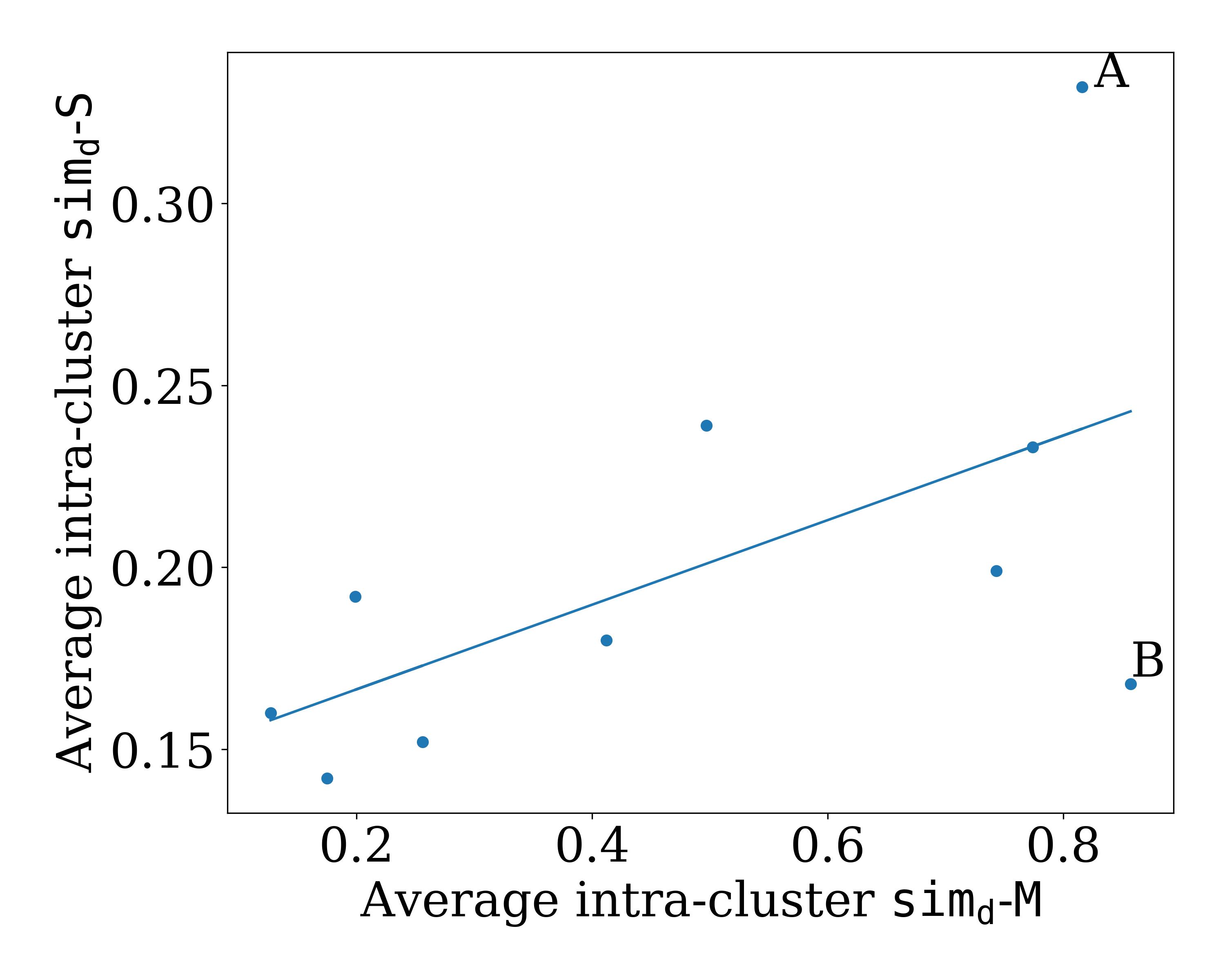
Figure 5. Scatter plot of intra-cluster similarities, computed as the average of $\mathop{\mathtt{sim_{d}\text{-}{S}}}\limits$ and $\mathop{\mathtt{sim_{d}\text{-}{M}}}\limits$ within each cluster.

We hypothesize that the learned latent space locally captures the sensitivity profiles of drugs. In other words, drugs that are close in the latent space have similar sensitivity profiles, leading to a correlation between the similarities in the latent space (i.e., $\mathop{\mathtt{sim_{d}\text{-}{B}}}\limits$ and $\mathop{\mathtt{sim_{d}\text{-}{M}}}\limits$) and those computed from the sensitivity profiles (i.e., $\mathop{\mathtt{sim_{d}\text{-}{S}}}\limits$). To test this hypothesis, we computed the Pearson correlations among the three similarities as follows: 1) correlation between $\mathop{\mathtt{sim_{d}\text{-}{B}}}\limits$ and $\mathop{\mathtt{sim_{d}\text{-}{S}}}\limits$, denoted as $\mathtt{corr_{d}(B,S)}$; and, 2) correlation between $\mathop{\mathtt{sim_{d}\text{-}{M}}}\limits$ and $\mathop{\mathtt{sim_{d}\text{-}{S}}}\limits$, denoted as $\mathtt{corr_{d}(M,S)}$. We observed that the pairwise drug similarities induced by cell sensitivity profiles are better correlated to the pairwise similarities induced in the latent space learned by $\mathop{\mathtt{List\text{-}All}}\limits$ compared to $\mathop{\mathtt{pLETORg}}\limits$ (Pearson correlations $\mathtt{corr_{d}(M,S)}$ and $\mathtt{corr_{d}(B,S)}$: 0.906 vs. 0.352). This suggests that $\mathop{\mathtt{List\text{-}All}}\limits$ can learn effective drug embeddings that can better capture the sensitivity profiles compared to $\mathop{\mathtt{pLETORg}}\limits$. This may be due to the fact that $\mathop{\mathtt{List\text{-}All}}\limits$ leverages molecular fingerprints, unlike $\mathop{\mathtt{pLETORg}}\limits$, to learn drug embeddings that can encode structural information; and it is well known that structurally similar drugs tend to exhibit similar sensitivities.

(a) Based on the distribution
of drugs across clusters.

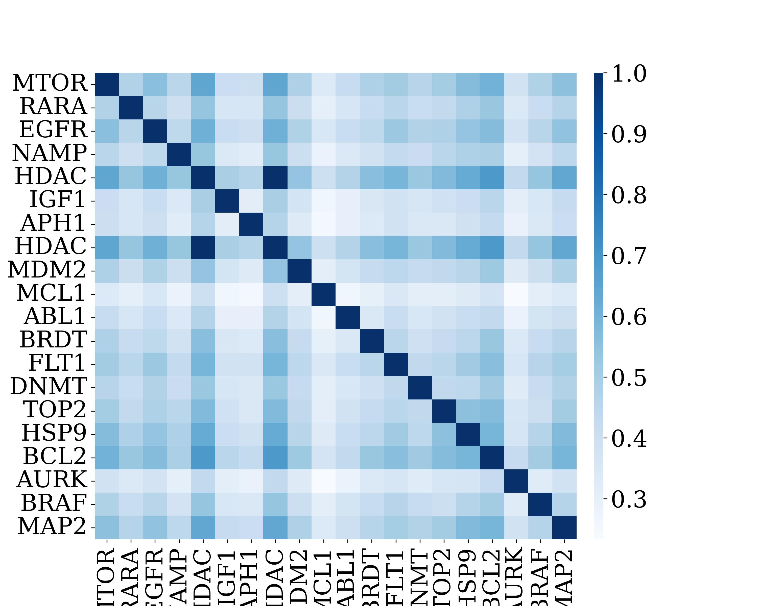
(b) Based on average $\mathop{\mathtt{sim_{d}\text{-}{S}}}\limits$
among drugs

Figure 6. Comparison of two pairwise similarity matrices across different MoAs.

Furthermore, we evaluated the quality of drug embeddings out of $\mathop{\mathtt{List\text{-}All}}\limits$ via clustering. We applied a 10-way clustering (using CLUTO) on the drug embeddings. Figure 5 presents the intra-cluster similarities, $\mathop{\mathtt{sim_{d}\text{-}{S}}}\limits$ vs. $\mathop{\mathtt{sim_{d}\text{-}{M}}}\limits$ averaged across all drugs in each cluster. We observed that the compact clusters in the latent space contained drugs with similar sensitivity profiles. This further supports our previous hypothesis that the latent space for drugs effectively captures the sensitivity profiles.

Furthermore, we studied the drug clusters in more detail and identified some qualities of the latent space with respect to uncovering the mechanism of action (MoA) of drugs. Figure 6a presents the average pairwise similarities among drugs grouped by different MoAs, where the similarities are computed using the Jaccard coefficient on the normalized distribution of drugs across clusters (Figure 5). In other words, if drugs with different MoAs are clustered together or co-occurs over multiple clusters, they are considered similar and have darker shades in the respective cells in this figure. Figure 6b presents the average pairwise $\mathop{\mathtt{sim_{d}\text{-}{S}}}\limits$ similarities among drugs with different MoAs. Notably, we find that certain MoAs, such as MTOR, RARA, EGFR, and NAMP, exhibit similarities in their clustering patterns, suggesting potential shared characteristics or pathways. Similarly, we observe similarities among ABL1, BRDT, and FLT1, as well as BCL2 and AURK. These findings might indicate potential commonalities among drugs with different MoAs, even when their sensitivity profiles may not be similar (Figure 6b).

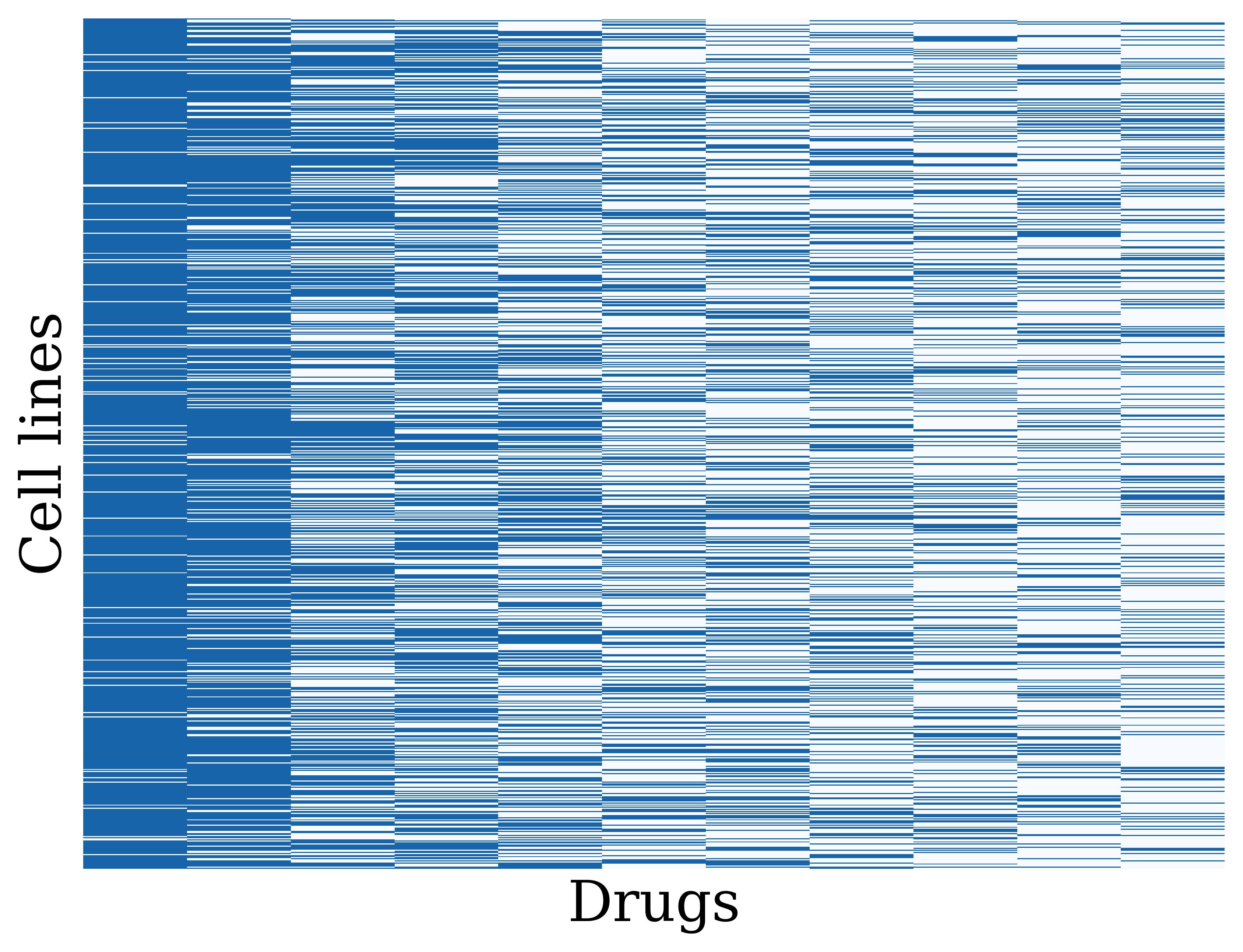
(a) Cluster A

(b) Cluster B

Figure 7. Comparison of sensitivity profiles for all drugs in clusters A and B in Figure 5. Darker color indicates that the drug is sensitive in corresponding cell lines.

We further examined clusters A and B depicted in Figure 5 to gain deeper insights into their characteristics. Despite both clusters being compact, they exhibit distinct characteristics in terms of their $\mathop{\mathtt{sim_{d}\text{-}{S}}}\limits$ similarities. Figure 7 presents the sensitivity profiles of all the drugs in each cluster. Clearly, compared to cluster B, most drugs in cluster A share multiple cell lines in which they are sensitive, thus resulting in higher $\mathop{\mathtt{sim_{d}\text{-}{S}}}\limits$ for cluster A than for cluster B. Specifically, from our preliminary fact-checking, we found that many drugs in cluster A (left-most drugs in Figure 7a) share some common pathways such as EGFR, mTOR. This suggests that these drugs possess broader effectiveness across multiple cancer types. In summary, our analysis reveals that the latent drug space learned by $\mathop{\mathtt{List\text{-}All}}\limits$ captures similarities in sensitivity profiles, molecular structures, and pathway mechanisms. These findings highlight the potential for exploring synergistic effects among drugs with different MoAs, and developing novel therapeutic strategies.

6. Conclusion

In this work, we developed two listwise neural ranking methods to select anti-cancer drugs out of all known drugs for new cell lines. Our experiments suggest that our listwise ranking method, $\mathop{\mathtt{List\text{-}All}}\limits$, can select all the sensitive drugs instead of the few top-most sensitive drugs. Moreover, our experimental comparison with strong ranking and regression baselines demonstrated the efficacy of formulating drug selection as a LeToR problem. Notably, our method, $\mathop{\mathtt{List\text{-}All}}\limits$ demonstrated significant improvements over the baseline $\mathop{\mathtt{pLETORg}}\limits$ in average hit rates across a large proportion of cell lines. Additionally, by leveraging deep networks and pretraining techniques, our methods can learn informative embeddings. Our analyses of such learned embeddings revealed commonalities among cell lines and among drugs from different cancer types and MoAs, respectively. Overall, our work represents a step forward in the development of robust and effective methods for precision anti-cancer drug selection. Future work may explore on leveraging 3D molecular structures, multiple modalities or pretrained chemical foundational models to further enhance ranking performance.

7. Code Availibility

The processed data and code are publicly available at https://github.com/ninglab/DrugRanker. All the required softwares to execute the code are freely available.

Appendix A Reproducibility

As the encoder $\mathop{\mathtt{GeneE}}\limits$, we used a fully-connected neural network consisting of 2 hidden layers with 4,096 and 1,024 units, respectively; each hidden layer is followed by a ReLU activation. The last hidden layer is followed by an output layer with 128 units which outputs the cell line latent embedding (from preliminary experiments, the best results were obtained with 128 units). We implemented $\mathop{\mathtt{DrugE}}\limits$ as a fully-connected neural network with one hidden layer of 128 hidden units followed by ReLU non-linearity, and the output layer of $M$ units, where $M\in\{25,50,100,200\}$. The hyperparameters for all the baselines and proposed methods were systematically fine-tuned via a random grid search. The learning rate and learning rate annealing scheme for $\mathop{\mathtt{pLETORg}}\limits$ were in accordance with its original implementation. Other methods were trained using ADAM optimization with an initial learning rate of 0.001. All the baselines were trained for 100 epochs or until the convergence of their respective training objectives. In contrast, the listwise ranking models were trained for 300 epochs. Each experiment was conducted on a computing node equipped with NVIDIA Volta V100 GPUs and Dual Intel Xeon 8268s processors. The hyperparameters for all the methods are reported in Table 4 to facilitate the reproducibility of results.

Table 4. Hyper-parameters used in grid search

Method	Hyper-parameter	Values
$\mathop{\mathtt{pLETORg}}\limits$	$l$	5, 10, 25, 50
	$\alpha$	0, 0.05, 0.1, 0.5, 1
	$\beta$	0.1, 1
	$\gamma$	0, 1, 10, 100
$\mathop{\mathtt{DeepCDR}}\limits$	$l$	25, 50, 100
$\mathop{\mathtt{DrugE}}\limits$	hidden_units	128, 256
	$M$	25, 50, 100

• $l$ denotes the dimension of the latent embeddings for $\mathop{\mathtt{pLETORg}}\limits$ and $\mathop{\mathtt{DeepCDR}}\limits$; $\alpha$, $\beta$ and $\gamma$ for $\mathop{\mathtt{pLETORg}}\limits$ refer to the original notations as used in (He et al., 2020);

References

- (1)
- Ananthakrishnan et al. (2006) Ashwin Ananthakrishnan, Veena Gogineni, and Kia Saeian. 2006. Epidemiology of Primary and Secondary Liver Cancers. Seminars in Interventional Radiology 23, 1 (March 2006), 047–063.
- Baptista et al. (2020) Delora Baptista, Pedro G Ferreira, and Miguel Rocha. 2020. Deep learning for drug response prediction in cancer. Briefings in Bioinformatics 22, 1 (Jan. 2020), 360–379.
- Barretina et al. (2012) Jordi Barretina, Giordano Caponigro, Nicolas Stransky, Kavitha Venkatesan, Adam A. Margolin, Sungjoon Kim, and et al. 2012. Nature 483, 7391 (March 2012), 603–607.
- Bickerton et al. (2012) G. Richard Bickerton, Gaia V. Paolini, Jérémy Besnard, Sorel Muresan, and Andrew L. Hopkins. 2012. Quantifying the chemical beauty of drugs. Nature Chemistry 4, 2 (Jan. 2012), 90–98.
- Bonanni et al. (2022) Davide Bonanni, Luca Pinzi, and Giulio Rastelli. 2022. Development of machine learning classifiers to predict compound activity on prostate cancer cell lines. Journal of Cheminformatics 14, 1 (Nov. 2022).
- Burges et al. (2005) Chris Burges, Tal Shaked, Erin Renshaw, Ari Lazier, Matt Deeds, Nicole Hamilton, and Greg Hullender. 2005. Learning to Rank Using Gradient Descent. In Proceedings of the 22nd International Conference on Machine Learning (Bonn, Germany) (ICML ’05). Association for Computing Machinery, New York, NY, USA, 89–96.
- Cao et al. (2007) Zhe Cao, Tao Qin, Tie-Yan Liu, Ming-Feng Tsai, and Hang Li. 2007. Learning to Rank: From Pairwise Approach to Listwise Approach (ICML ’07). Association for Computing Machinery, New York, NY, USA, 129–136.
- Davis et al. (2014) Elizabeth J. Davis, Jennifer L. Beebe-Dimmer, Cecilia L. Yee, and Kathleen A. Cooney. 2014. Risk of second primary tumors in men diagnosed with prostate cancer: A population-based cohort study. Cancer 120, 17 (2014), 2735–2741.
- Dincer et al. (2020) Ayse B Dincer, Joseph D Janizek, and Su-In Lee. 2020. Adversarial deconfounding autoencoder for learning robust gene expression embeddings. Bioinformatics 36, Supplement 2 (Dec. 2020), i573–i582.
- Erhan et al. (2010) Dumitru Erhan, Aaron Courville, Yoshua Bengio, and Pascal Vincent. 2010. Why Does Unsupervised Pre-training Help Deep Learning?. In Proceedings of the Thirteenth International Conference on Artificial Intelligence and Statistics (Proceedings of Machine Learning Research, Vol. 9). PMLR, 201–208.
- Fan et al. (2017) Chao-Yueh Fan, Wen-Yen Huang, Chun-Shu Lin, Yu-Fu Su, Cheng-Hsiang Lo, Chih-Cheng Tsao, and et al. 2017. Risk of second primary malignancies among patients with prostate cancer: A population-based cohort study. PLOS ONE 12, 4 (04 2017), 1–11.
- Firoozbakht et al. (2021) Farzaneh Firoozbakht, Behnam Yousefi, and Benno Schwikowski. 2021. An overview of machine learning methods for monotherapy drug response prediction. Briefings in Bioinformatics 23, 1 (Oct. 2021).
- Gerdes et al. (2021) Henry Gerdes, Pedro Casado, Arran Dokal, Maruan Hijazi, Nosheen Akhtar, Ruth Osuntola, Vinothini Rajeeve, and et al. 2021. Drug ranking using machine learning systematically predicts the efficacy of anti-cancer drugs. Nature Communications 12, 1 (March 2021).
- Gillet et al. (1998) Valerie J. Gillet, Peter Willett, and John Bradshaw. 1998. Identification of Biological Activity Profiles Using Substructural Analysis and Genetic Algorithms. Journal of Chemical Information and Computer Sciences 38, 2 (1998), 165–179.
- Gupta et al. (2009) Piyush B. Gupta, Tamer T. Onder, Guozhi Jiang, Kai Tao, Charlotte Kuperwasser, Robert A. Weinberg, and Eric S. Lander. 2009. Identification of Selective Inhibitors of Cancer Stem Cells by High-Throughput Screening. Cell 138, 4 (2009), 645–659.
- He et al. (2018) Xiao He, Lukas Folkman, and Karsten Borgwardt. 2018. Kernelized rank learning for personalized drug recommendation. Bioinformatics 34, 16 (03 2018), 2808–2816.
- He et al. (2020) Yicheng He, Junfeng Liu, and Xia Ning. 2020. Drug Selection via Joint Push and Learning to Rank. IEEE/ACM Trans. Comput. Biol. Bioinformatics 17, 1 (jan 2020), 110–123.
- Kandoth et al. (2013) Cyriac Kandoth, Michael D. McLellan, Fabio Vandin, Kai Ye, Beifang Niu, Charles Lu, and et al. 2013. Mutational landscape and significance across 12 major cancer types. Nature 502, 7471 (Oct. 2013), 333–339.
- Karypis (2002) George Karypis. 2002. CLUTO - A Clustering Toolkit. https://hdl.handle.net/11299/215521
- Khemlina et al. (2017) Galina Khemlina, Sadakatsu Ikeda, and Razelle Kurzrock. 2017. The biology of Hepatocellular carcinoma: implications for genomic and immune therapies. Molecular Cancer 16, 1 (aug 2017).
- Lipinski et al. (2001) Christopher A Lipinski, Franco Lombardo, Beryl W Dominy, and Paul J Feeney. 2001. Experimental and computational approaches to estimate solubility and permeability in drug discovery and development settings. Advanced Drug Delivery Reviews 46, 1 (2001), 3–26.
- Liu et al. (2020) Qiao Liu, Zhiqiang Hu, Rui Jiang, and Mu Zhou. 2020. DeepCDR: a hybrid graph convolutional network for predicting cancer drug response. Bioinformatics 36 (12 2020), i911–i918.
- Perkins et al. (2003) Roger Perkins, Hong Fang, Weida Tong, and William J. Welsh. 2003. Quantitative structure-activity relationship methods: Perspectives on drug discovery and toxicology. Environmental Toxicology and Chemistry 22, 8 (2003), 1666–1679.
- Prasse et al. (2022) Paul Prasse, Pascal Iversen, Matthias Lienhard, Kristina Thedinga, Chris Bauer, Ralf Herwig, and Tobias Scheffer. 2022. Matching anticancer compounds and tumor cell lines by neural networks with ranking loss. NAR Genomics and Bioinformatics 4, 1 (01 2022).
- Riihimäki et al. (2018) Matias Riihimäki, Hauke Thomsen, Kristina Sundquist, Jan Sundquist, and Kari Hemminki. 2018. Clinical landscape of cancer metastases. Cancer Medicine 7, 11 (Oct. 2018), 5534–5542.
- Rogers and Hahn (2010) David Rogers and Mathew Hahn. 2010. Extended-Connectivity Fingerprints. Journal of Chemical Information and Modeling 50, 5 (April 2010), 742–754.
- Seashore-Ludlow et al. (2015) Brinton Seashore-Ludlow, Matthew G. Rees, Jaime H. Cheah, Murat Cokol, Edmund V. Price, Matthew E. Coletti, and et al. 2015. Harnessing Connectivity in a Large-Scale Small-Molecule Sensitivity Dataset. Cancer Discovery 5, 11 (11 2015), 1210–1223.
- Su et al. (2019) Ran Su, Xinyi Liu, Guobao Xiao, and Leyi Wei. 2019. Meta-GDBP: a high-level stacked regression model to improve anticancer drug response prediction. Briefings in Bioinformatics 21, 3 (03 2019), 996–1005.
- Tomaszewski et al. (2014) Jeffrey J. Tomaszewski, Robert G. Uzzo, Brian Egleston, Anthony T. Corcoran, Reza Mehrazin, Daniel M. Geynisman, John A. Ridge, and et al. 2014. Coupling of Prostate and Thyroid Cancer Diagnoses in the United States. Annals of Surgical Oncology 22, 3 (Sept. 2014), 1043–1049.
- Wang et al. (2017) Lin Wang, Xiaozhong Li, Louxin Zhang, and Qiang Gao. 2017. Improved anticancer drug response prediction in cell lines using matrix factorization with similarity regularization. BMC Cancer 17, 1 (Aug. 2017).
- Weinstein et al. (2013) John N Weinstein, Eric A Collisson, Gordon B Mills, Kenna R Mills Shaw, Brad A Ozenberger, Kyle Ellrott, and et al. 2013. The Cancer Genome Atlas Pan-Cancer analysis project. Nature Genetics 45, 10 (Sept. 2013), 1113–1120.
- Wu et al. (2021) Zonghan Wu, Shirui Pan, Fengwen Chen, Guodong Long, Chengqi Zhang, and Philip S. Yu. 2021. A Comprehensive Survey on Graph Neural Networks. IEEE Transactions on Neural Networks and Learning Systems 32, 1 (2021), 4–24.
- Xie et al. (2017) Rui Xie, Jia Wen, Andrew Quitadamo, Jianlin Cheng, and Xinghua Shi. 2017. A deep auto-encoder model for gene expression prediction. BMC Genomics 18, S9 (Nov. 2017).
- Yang et al. (2012) Wanjuan Yang, Jorge Soares, Patricia Greninger, Elena J. Edelman, Howard Lightfoot, Simon Forbes, and et al. 2012. Genomics of Drug Sensitivity in Cancer (GDSC): a resource for therapeutic biomarker discovery in cancer cells. Nucleic Acids Research 41, D1 (11 2012), D955–D961.
- Zhang et al. (2022) Zehong Zhang, Lifan Chen, Feisheng Zhong, Dingyan Wang, Jiaxin Jiang, Sulin Zhang, and et al. 2022. Graph neural network approaches for drug-target interactions. Current Opinion in Structural Biology 73 (2022), 102327.
- Zuo et al. (2021) Zhaorui Zuo, Penglei Wang, Xiaowei Chen, Li Tian, Hui Ge, and Dahong Qian. 2021. SWnet: a deep learning model for drug response prediction from cancer genomic signatures and compound chemical structures. BMC Bioinformatics 22, 1 (Sept. 2021).