Band gaps of long-period polytypes of IV, IV-IV, and III-V semiconductors estimated with an Ising-type additivity model

Abstract

We apply an Ising-type model to estimate the band gaps of the polytypes of group IV elements (C, Si, and Ge) and binary compounds of groups: IV-IV (SiC, GeC, and GeSi), and III-V (nitride, phosphide, and arsenide of B, Al, and Ga). The models use reference band gaps of the simplest polytypes comprising 2–6 bilayers calculated with the hybrid density functional approximation, HSE06. We report four models capable of estimating band gaps of nine polytypes containing 7 and 8 bilayers with an average error of $\lesssim 0.05$ eV. We apply the best model with an error of $<0.04$ eV to predict the band gaps of 497 polytypes with up to 15 bilayers in the unit cell, providing a comprehensive view of the variation in the electronic structure with the degree of hexagonality of the crystal structure. Within our enumeration, we identify four rhombohedral polytypes of SiC—9$R$, 12$R$, 15$R$(1), and 15$R$(2)—and perform detailed stability and band structure analysis. Of these, 15$R$(1) that has not been experimentally characterized has the widest band gap ($>3.4$ eV); phonon analysis and cohesive energy reveal 15$R$(1)-SiC to be metastable. Additionally, we model the energies of valence and conduction bands of the rhombohedral SiC phases at the high-symmetry points of the Brillouin zone and predict band structure characteristics around the Fermi level. The models presented in this study may aid in identifying polytypic phases suitable for various applications, such as the design of wide-gap materials, that are relevant to high-voltage applications. In particular, the method holds promise for forecasting electronic properties of long-period and ultra-long-period polytypes for which accurate first-principles modeling is computationally challenging.

I Introduction

The fundamental gap (or the transport gap) of a material is the difference between its ionization energy and electron affinity: $E_{g}={\rm IP}-{\rm EA}$. For an $N$-electron system, $E_{g}$ can be formally expressed as $E_{g}=E\left(N+1\right)+E\left(N-1\right)-2E\left(N\right)$, where $E$ is the total energy. Within the Kohn–Sham (KS) formalism of density functional theory (DFT), $E_{g}$ is approximated by the KS gap, which is the difference between the energy of the conduction band minimum (CBM) and that of the valence band maximum (VBM): $\varepsilon_{g}^{\rm KS}=\varepsilon_{\rm CMB}-\varepsilon_{\rm VBM}$Perdew et al. (2017). The difference $E_{g}-\varepsilon_{g}^{\rm KS}=\Delta_{\rm XC}$ is called the derivative discontinuity of the exchange-correlation (XC) contribution to the total energyPerdew and Levy (1983). Typically, $\Delta_{\rm XC}>0$ for semi-local KS-DFT methods—local-density approximation (LDA), generalized gradient approximation (GGA), and meta-generalized gradient approximation (mGGA)—resulting in the underestimation of a material’s fundamental gapPerdew and Ruzsinszky (2018). As stated by John P. Perdew et al., even with the exact KS band structure, $\varepsilon_{g}$ will underestimate $E_{g}$,Perdew and Ruzsinszky (2010) as the former approximates the first exciton energy, while the latter, the asymptotic limit of a Rydberg series of exciton energiesPerdew et al. (2009). The Hartree–Fock method, with 100% exact exchange, has been known to overestimate $E_{g}$, often predicting paramagnetic metals as antiferromagnetic insulatorsMizokawa and Fujimori (1996). Hence, KS-DFT with a hybrid-XC treatmentHeyd et al. (2003); Krukau et al. (2006), which includes a fraction of the exact exchange energy, offers a more realistic description of $E_{g}$ due to favorable error cancellationsPerdew et al. (1996a).

Table 1: Definitions of small polytypes considered in this study: Stacking sequence in close-packing, $hk$, and Hägg notations are given. Polytype names (in Ramsdell notation) and space group details are given separately for compounds and elements. Names of binary compounds are used in the text for all systems. Also given is a crystal structure’s degree of hexagonality (%hex). For 3$C$, space group details for a non-primitive rhombohedral unit cell in the hexagonal lattice are also given.

Stacking sequence				Binary compounds			Elements			%hex
Close-packing	$hk$	Hägg		Name	Space group		Name	Space group
AB	hh	$+-$		2$H$	P$6_{3}$mc (186)		2$H$	P$6_{3}$/mmc (194)		100
ABC	kkk	$+++$		3$C$ / 3$R$	F$\overline{4}$3m (216) / R$\overline{3}$m (166)		3$C$ /3$R$	Fd$\overline{3}$m (227) /R3m (160)		0
ABAC	hkhk	$+--+$		4$H$	P$6_{3}$mc (186)		4$H$	P$6_{3}$/mmc (194)		50
ABABC	hhkkk	$+-+++$		5$T$	P3m1 (156)		5$T$	P$\overline{3}$m1 (164)		40
ABABAC	hhhkhk	$+-+--+$		6$T$	P3m1 (156)		6$H$(1)	P$\overline{6}$m$2$ (187)		66.67
ABACBC	hkkhkk	$+---++$		6$H$	P$6_{3}$mc (186)		6$H$(2)	P$6_{3}$/mmc (194)		33.33
ABABABC	hhhhkkk	$+-+-+++$		7$T$(1)	P3m1 (156)		7$T$(1)	P$\overline{3}$m1 (164)		57.14
ABABCAC	hhkhhkk	$+-+++-+$		7$T$(2)	P3m1 (156)		7$T$(2)	P$\overline{3}$m1 (164)		57.14
ABACABC	hkhkkkk	$+--++++$		7$T$(3)	P3m1 (156)		7$T$(3)	P$\overline{3}$m1 (164)		28.57
ABABABAC	hhhhhkhk	$+-+-+--+$		8$T$(1)	P3m1 (156)		8$H$(1)	P$\overline{6}$m$2$ (187)		75
ABABACAC	hhhkhhhk	$+-+--+-+$		8$H$(1)	P$6_{3}$mc (186)		8$H$(2)	P$6_{3}$/mmc (194)		75
ABABACBC	hhhkkhkk	$+-+---++$		8$T$(2)	P3m1 (156)		8$H$(3)	P$\overline{6}$m$2$ (187)		50
ABABCABC	hhkkkkkk	$+-++---+$		8$T$(3)	P3m1 (156)		8$T$(1)	P$\overline{3}$m1 (164)		25
ABABCBAC	hhkhkkhk	$+-++++++$		8$T$(4)	P3m1 (156)		8$T$(2)	P$\overline{3}$m1 (164)		50
ABACBABC	hkkkhkkk	$+----+++$		8$H$(2)	P$6_{3}$mc (186)		8$H$(4)	P$6_{3}$/mmc (194)		25

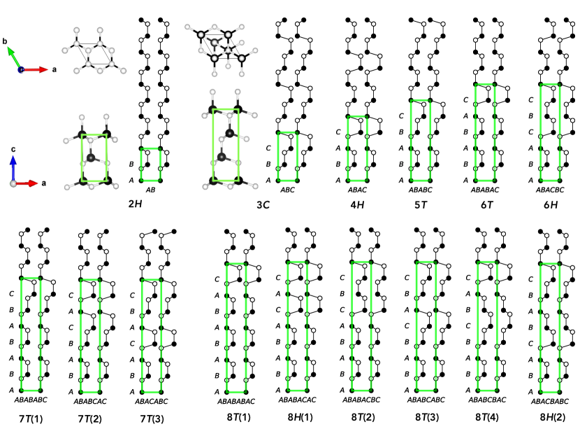
Figure 1: Stacking arrangement of polytypes with up to 8 bilayers as viewed from the [10$\overline{1}$0] plane of the hexagonal unit cell. For 2$H$ and 3$C$, side and top views of a ball-and-stick representation are shown for comparison. For binary compounds, white and black circles correspond to different atom types, while for elements, they correspond to the same atom type. The unit cell is shown in a green rectangle.

Range-separated hybrid XC functionals are highly effective in accurately predicting the experimental band gaps of semiconductors, with minimal systematic errors, but they are not suitable for modeling metalsPerdew and Ruzsinszky (2018). Furthermore, applying hybrid XC methods for large unit cell systems becomes impractical due to their high computational cost. As a result, alternative surrogate methods incorporating empirical parameters to estimate hybrid DFT-level band gaps are finding increased applications. The $\Delta-$sol method estimates $E_{g}$ as the finite derivative of the energy ($E$) with respect to an empirically determined fraction of valence electrons in the unit cellChan and Ceder (2010). A popular empirical approach is the DFT+U method, where a Hubbard-type energy correction term improves the accuracy of the band gap ($\varepsilon_{g}$), particularly for strongly localized bandsVerma and Truhlar (2016); Ramakrishnan et al. (2009); Kulik (2015). Morales et al.Morales-García et al. (2017) employed linear regression using reference results from the many-body perturbation theory (GW) for a representative “training set” to enhance the accuracy of GGA level $\varepsilon_{g}$ for a “test set” of semiconductors. More rigorous methods based on machine learning (ML) use GGA-level $\varepsilon_{g}$ as input features to predict GW-level resultsLee et al. (2016). For the same task, non-linear regressions based on neural networks offer better performancesNa et al. (2020). ML models can also predict hybrid-DFT level $\varepsilon_{g}$ using the GGA-level electron density as a featureMoreno et al. (2021); Lentz and Kolpak (2020). Models have also been trained on the difference between $\varepsilon_{g}$ from hybrid-DFT and GGA methodsZhang et al. (2022) using the $\Delta-$ML approachRamakrishnan et al. (2015), which effectively provide non-systematic corrections to GGA with increased training. ML models of $\varepsilon_{g}$ show high accuracy when trained on narrow property rangesBorlido et al. (2020), indicating that for a given composition, electronic properties such as $\varepsilon_{g}$ exhibit slight variations from a mean value with gradual changes of configuration variables in the materials space. Consequently, empirical models of $\varepsilon_{g}$ designed for specific classes of materials hold significant potential for various applications.

In this study, we explore the application of an additivity model inspired by the cluster expansion of the Ising modelWu et al. (2016). This approach can very accurately determine the energies of compounds within a consistent compound spaceLaks et al. (1992). The Ising model exploits near-sightedness in chemical interactions and is very efficient for modeling the energetics of spatially modulated phasesElliott (1961). Individual interacting units can be atoms or molecules in a lattice or sub-units of the bulk crystal, such as layers. Specifically, when the model focuses on phases that exhibit modulation of charge density along an axis perpendicular to a layered structure, it is referred to as the axial next-nearest-neighbor-interaction (ANNNI) model or the ANNNI-Ising modelSelke (1988), referred hereafter as the Ising-type model.

Using reference energies of small unit cell phases calculated using first-principles methods, the Ising-type model has demonstrated high accuracy in predicting the relative energies of larger unit cell phases, achieving less than milli-electron volt (meV) accuracy Limpijumnong and Lambrecht (1998); Panse et al. (2011); Raffy et al. (2002); Moriguchi et al. (2021); Keller et al. (2023); Kobayashi and Komatsu (2012); Moriguchi et al. (2013); Bechstedt and Belabbes (2013). This approach aids in understanding the phase diagram or the relative thermodynamic stabilities of the polytypes of layered compoundsSmith et al. (1984); Trigunayat (1991), particularly silicon carbide (SiC)Heine (1985); Cheng et al. (1989, 1990). These phenomenological models do not account for the dynamic stability of a long-period polytype based on phonon band structure diagnosticsKayastha and Ramakrishnan (2021); Pallikara et al. (2022).

In our study, we aim to assess the applicability of the Ising Ansatz as a mathematical representation for modeling $\varepsilon_{g}$ across the polytypes of group IV elements (C, Si, and Ge), IV-IV (SiC, GeC, and GeSi), and III-V binary compounds (BN, BP, BAs, AlN, AlP, AlAs, GN, GaP, GaAs). The model is applied for each composition to estimate the band gaps of 497 polytypes containing up to 15 bilayers in the unit cell. Furthermore, we analyze the trends in band gaps with the hexagonality of the crystal structure and conduct a more comprehensive analysis focusing on the rhombohedral phases of SiC more commonly encountered in experimental studies. Finally, we explore the scope to develop models of the energies of valence and conduction bands at the high-symmetry points in the Brillouin zone to rapidly generate the band structure characteristics of polytypes around the Fermi level.

II Theory

Polytypism is a particular case of polymorphism where structural variations arise from the stacking sequence of layered units along an axis perpendicular to the layers. Three-dimensional structural information, such as lattice parameters and Wyckoff positions, of many polytypes are well documentedRohrer (2001); Tilley (2020); Bechstedt and Belabbes (2013); Halac et al. (2002). However, for a complete enumeration of structures, an algorithmic approach to cover the entire compound space spanned by polytypes is necessary. Pólya enumeration is a powerful algebraic technique used to derive closed-form expressions for the number of equivalent patterns, eliminating the need for explicit structure constructionPolya and Read (2012). This method has been successfully employed for various problems, including the generation of a comprehensive catalogue of heteroatom-substituted benzenoid compounds Chakraborty et al. (2019) and other compounds Douglas and Hollingsworth (2012); Müller (2013). However, explicit construction and de-duplication are necessary to identify unique structures when dealing with three-dimensional structures. For rapid enumeration using combinatorial techniques, structures can also be represented as string-based fingerprints.

A previous studyMcLarnan (1981) has enumerated distinct close-packings and polytypes. To generate the corresponding sequenceLothaire (1997), Jagodzinski’s $hk$-notation is employed Guinier et al. (1984). In this notation, a letter $h$ denotes layers sandwiched between similar layers, as in hexagonal close-packing, while $k$ denotes layers sandwiched between different neighbors, representing a local cubic structure. From the $hk$ sequence, we obtained the close-packing sequence and also calculated the percentage of the locally hexagonal layers, $\%{\rm hex}=100\times\#h/\left(\#h+\#k\right)$, where # indicates the count. For the simplest 15 polytypes of elements and binary compounds containing up to 8 bilayers (i.e. formula units), Table 1 provides the stacking sequence in various notations, space group details, and %hex. FIG. 1 presents the schematic representations of the corresponding stacking arrangements.

In the case of binary semiconductors, where the formula unit comprises two different types of atoms, the corresponding space group becomes a “Klassengleiche” subgroup of the elemental phase’s space group (see Table 1). The polytypes are named using the Ramsdell notationRamsdell (1947), denoted as $pY(z)$. Here, $p$ represents the number of bilayers in the unit cell, and $Y$ signifies the crystal class ($C$: cubic, $H$: hexagonal, $T$: trigonal, or $R$: rhombohedral). The number $z$ in parentheses indicates the index. In this study, we arranged the polytypes in lexicographic order based on their close-packing sequence. For instance, the 7$H$ polytypes, namely $ABABABC$, $ABABCAC$, and $ABACABC$, are assigned indices 1, 2, and 3, respectively (see Table 1). The 3$C$ polytype has the cubic zincblende structure and 2$H$ polytype corresponds to the hexagonal wurtzite structure. We provide the details of long-period polytypes with many bilayers at the relevant places in the text.

For Ising-type models, we require a numerical representation that forms a bijective mapping to the close-packing sequence. The Hägg representationGuinier et al. (1984, 1984); Ortiz et al. (2013) achieves this, where a layer (or bilayer when the formula unit has two atoms) is assigned a pseudo-spin value of $\sigma_{i}=+1$ when the layer above is in the order $A\rightarrow B$, $B\rightarrow C$, or $C\rightarrow A$. When the sequence moves as $B\rightarrow A$, $C\rightarrow B$, or $A\rightarrow C$, the assignment is $\sigma_{i}=-1$. As a shorthand notation, only the signs of $\sigma_{i}$ are given in TABLE 1. The mapping of a bilayer’s local structure to a pseudospin value is shown for the 4$H$ polytype in FIG. 2. The simplest model studied here contains four parameters:

$$\varepsilon_{g} = J_{0}-J_{1}\langle\sigma_{i}\sigma_{i+1}\rangle-J_{2}\langle\sigma_{i}\sigma_{i+2}\rangle-J_{3}\langle\sigma_{i}\sigma_{i+3}\rangle$$ (1)

While there are no formal constraints on increasing the number of interaction terms in Eq. (1), we aim to develop a simple model suitable for a rapid analysis of its performance. The first coefficient, $J_{0}$, corresponds to an intercept of a hyperplane in the model space. When the inter-layer interactions are negligible in the polytypes, the model will predict $\varepsilon_{g}$ to be $J_{0}$ for all polytypes. The ‘2-body’ interaction terms $\langle\sigma_{i}\sigma_{i+1}\rangle$, $\langle\sigma_{i}\sigma_{i+2}\rangle$, and $\langle\sigma_{i}\sigma_{i+3}\rangle$ correspond to the interaction of layer-$i$ with the first, second, and third layers, respectively.

The notation $\langle x\rangle$ implies averaging over all layers in the unit cell, $(1/p)\sum_{i=1}^{p}x_{i}$, for a given polytype comprising $p$ bilayers. For example, for the 4$H$ polytype (with four bilayers, $p=4$), the first neighbor interaction term is evaluated as

$$\langle\sigma_{i}\sigma_{i+1}\rangle=\frac{1}{4}\left[\sigma_{1}\sigma_{2}+\sigma_{2}\sigma_{3}+\sigma_{3}\sigma_{4}+\sigma_{4}\sigma_{5}\right].$$ (2)

For the 4$H$ polytype, $i=5$ corresponds to $i=1$ by periodicity. Inserting the pseudo-spin values shown in FIG. 2 in Eq. (2), we find

$$\frac{1}{4}\left[(1)(-1)+(-1)(-1)+(-1)(1)+(1)(1)\right]=0.$$ (3)

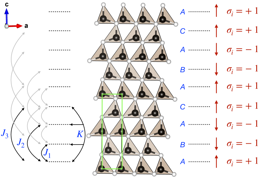
Figure 2: ABAC stacking sequence of 4$H$ polytype mapped to an arrangement of spins. Each row of pyramids corresponds to a bilayer in the ${\bf a}$-${\bf b}$ plane. The pseudo-spin value of a bilayer is $\sigma_{i}=+1$ (symbolically mapped to the ‘up’ spin) when a layer and the one above follows the order $A\rightarrow B$, $B\rightarrow C$, or $C\rightarrow A$. When the sequence is reversed as $B\rightarrow A$, $C\rightarrow B$, or $A\rightarrow C$, the pseudo-spin value of a bilayer is $\sigma_{i}=-1$ (i.e. ‘down’ spin). First, second and third-neighbor 2-body and 4-body interactions are shown.

For SiC, the unknown coefficients $J_{0-3}$ were obtained by a linear regression using the HSE06 band gaps of 2$H$, 3$C$, 4$H$, and 6$H$ polytypes. We denote the resulting model as Model-1. Since we aim to identify structure-property correlations across the compound space of polytypes, we select the reference systems for determining the models’ parameters without any experimental bias. To this end, we evaluate the model’s performance by applying it to nine long-period polytypes: 7$H$(1-3), 8$H$(1-2), and 8$T$(1-4) listed in TABLE 1. We also explore replacing 6$H$ with 6$T$, resulting in Model-2. We note in passing that using the 5$T$ polytype in a 4-parameter model with only 2-body terms along with 2$H$, 3$C$, and 4$H$ resulted in linear dependency because the 2-body interaction terms of 3$C$ are proportional to that of 5$T$ (see TABLE 2).

We have also tested the role of a ‘4-body’ term $\langle\sigma_{i}\sigma_{i+1}\sigma_{i+2}\sigma_{i+3}\rangle$. As previously discussedCheng et al. (1988), for polytypes of elements and binary compounds, odd terms such as the 3-body terms vanish due to permutation symmetry. However, these terms play a role in modeling the relative energies of polytypes of other compoundsPrice and Yeomans (1984); Plumer et al. (1988). We augment both Model-1 and Model-2 with a 4-body term by including the 5$T$ polytype to arrive at Model-3 and Model-4 containing five unknown parameters:

$$\varepsilon_{g} = J_{0}-J_{1}\langle\sigma_{i}\sigma_{i+1}\rangle-J_{2}\langle\sigma_{i}\sigma_{i+2}\rangle-J_{3}\langle\sigma_{i}\sigma_{i+3}\rangle$$ (4)

$$-K\langle\sigma_{i}\sigma_{i+1}\sigma_{i+2}\sigma_{i+3}\rangle$$

Table 2 provides numerical values of the interaction terms for several polytypes. These terms are property-independent; hence, for SiC, we have applied the same interaction terms to determine $J_{0-3}$ and $K$ for modeling the energies of VB and CB at the high-symmetry points of the Brillouin zone. In this case, the model parameters will be implicit functions of these $k$ points.

Table 2: Terms in the model of $\varepsilon_{g}$ given in Eq. (1) and Eq. (4) for various polytypes.

Polytype	$\langle\sigma_{i}\sigma_{i+1}\rangle$	$\langle\sigma_{i}\sigma_{i+2}\rangle$	$\langle\sigma_{i}\sigma_{i+3}\rangle$	$\langle\sigma_{i}\sigma_{i+1}\sigma_{i+2}\sigma_{i+3}\rangle$
2$H$	-1	1	-1	1
3$C$	1	1	1	1
4$H$	0	-1	0	1
5$T$	1/5	1/5	1/5	-3/5
6$T$	-1/3	-1/3	1/3	1/3
6$H$	1/3	-1/3	-1	-1/3
7$H$(1)	-1/7	3/7	-1/7	-1/7
7$H$(2)	-1/7	-1/7	3/7	-5/7
7$H$(3)	3/7	-1/7	-1/7	3/7
8$H$(1)	-1/2	0	0	1/2
8$T$(1)	-1/2	0	1/2	0
8$T$(2)	0	0	-1/2	-1/2
8$T$(3)	1/2	1/2	1/2	0
8$T$(4)	0	-1/2	0	0
8$H$(2)	1/2	0	-1/2	0
9$R$	-1/3	-1/3	1	-1/3
12$R$	0	0	0	-1
15$R$(1)	-3/5	1/5	1/5	1/5
15$R$(2)	1/5	-3/5	-3/5	1/5

III Results and Discussions

III.1 Structural and electronic properties

GGA-PBE minimum energy crystal structures of the simplest 15 polytypes of all semiconductors studied in this work are given in Table S1 and Table S2 in the Supporting Information (SI). For all structures, the $x$ and $y$ fractional coordinates (i.e. $x$ and $y$ Wyckoff coordinates) remain in their ideal positions, as in the corresponding composition’s wurtzite phase. In our investigation of 225 systems, encompassing 15 polytypes and 15 compositions, we observed minimal deviations from the ideal positions ($u_{i}$ and $v_{i}$ stated in IV.1), measuring less than $10^{-3}$ Å. It is worth noting that such minor deviations have proven to be significant for accurately refining experimental crystal structures Gomes de Mesquita (1967); Bauer et al. (1998). However, given that these deviations are 2 or 3 orders of magnitude smaller than the uncertainty in the GGA-PBE lattice constants compared to experimental ones, we have not focused on $u_{i}$ and $v_{i}$.

Table 3: Band gaps (in eV) of 15 polytypes of semiconductors calculated with PBE, SCAN, and HSE06 DFT methods using PBE equilibrium crystal structure. The band gap character is denoted as $d$ for direct and $i$ for indirect.

Sys.	XC	2$H$	3$C$	4$H$	5$T$	6$T$	6$H$	7$T$(1)	7$T$(2)	7$T$(3)	8$T$(1)	8$H$(1)	8$T$(2)	8$T$(3)	8$T$(4)	8$H$(2)
C	PBE	3.58 $i$	4.18 $i$	4.58 $i$	4.35 $i$	4.51 $i$	4.42 $i$	4.29 $i$	4.45 $i$	4.37 $i$	4.13 $i$	4.42 $i$	4.47 $i$	4.24 $i$	4.46 $i$	4.39 $i$
	SCAN	4.00 $i$	4.59 $i$	4.99 $i$	4.75 $i$	4.95 $i$	4.82 $i$	4.73 $i$	4.85 $i$	4.78 $i$	4.57 $i$	4.87 $i$	4.87 $i$	4.64 $i$	4.86 $i$	4.79 $i$
	HSE06	4.74 $i$	5.41 $i$	5.82 $i$	5.59 $i$	5.73 $i$	5.66 $i$	5.49 $i$	5.69 $i$	5.61 $i$	5.33 $i$	5.64 $i$	5.71 $i$	5.48 $i$	5.70 $i$	5.62 $i$
Si	PBE	0.48 $i$	0.66 $i$	0.63 $i$	0.61 $i$	0.56 $i$	0.64 $i$	0.57 $i$	0.58 $i$	0.67 $i$	0.54 $i$	0.54 $i$	0.60 $i$	0.64 $i$	0.60 $i$	0.68 $i$
	SCAN	0.72 $i$	0.90 $i$	0.87 $i$	0.85 $i$	0.80 $i$	0.88 $i$	0.81 $i$	0.82 $i$	0.91 $i$	0.77 $i$	0.78 $i$	0.83 $i$	0.88 $i$	0.84 $i$	0.92 $i$
	HSE06	1.05 $i$	1.24 $i$	1.21 $i$	1.19 $i$	1.14 $i$	1.22 $i$	1.15 $i$	1.15 $i$	1.26 $i$	1.11 $i$	1.12 $i$	1.17 $i$	1.22 $i$	1.18 $i$	1.26 $i$
Ge	PBE	0.06 $i$	0.03 $i$	0.08 $i$	0.03 $i$	0.05 $i$	0.06 $i$	0.04 $i$	0.07 $i$	0.08 $i$	0.05 $i$	0.02 $i$	0.01 $i$	0.02 $i$	0.01 $i$	0.03 $i$
	SCAN	0.13 $d$	0.04 $d$	0.12 $d$	0.04 $d$	0.07 $d$	0.06 $d$	0.08 $d$	0.03 $d$	0.06 $d$	0.04 $d$	0.08 $d$	0.06 $d$	0.03 $d$	0.02 $d$	0.00 $d$
	HSE06	0.12 $d$	0.15 $d$	0.18 $d$	0.17 $d$	0.16 $d$	0.18 $d$	0.15 $d$	0.16 $d$	0.18 $d$	0.15 $d$	0.15 $d$	0.16 $d$	0.18 $d$	0.17 $d$	0.19 $d$
SiC	PBE	2.33 $i$	1.54 $i$	2.35 $i$	1.87 $i$	2.38 $i$	2.13 $i$	1.90 $i$	2.10 $i$	1.81 $i$	2.42 $i$	2.33 $i$	2.06 $i$	1.65 $i$	2.14 $i$	1.90 $i$
	SCAN	2.70 $i$	1.88 $i$	2.70 $i$	2.22 $i$	2.75 $i$	2.48 $i$	2.25 $i$	2.46 $i$	2.15 $i$	2.80 $i$	2.70 $i$	2.41 $i$	2.00 $i$	2.50 $i$	2.25 $i$
	HSE06	3.29 $i$	2.50 $i$	3.34 $i$	2.84 $i$	3.38 $i$	3.10 $i$	2.87 $i$	3.09 $i$	2.77 $i$	3.42 $i$	3.33 $i$	3.04 $i$	2.62 $i$	3.12 $i$	2.87 $i$
GeC	PBE	2.42 $i$	1.80 $i$	2.16 $i$	1.96 $i$	2.18 $i$	2.13 $i$	2.00 $i$	2.09 $i$	1.95 $i$	2.22 $i$	2.17 $i$	2.08 $i$	1.88 $i$	2.13 $i$	2.02 $i$
	SCAN	2.66 $i$	2.03 $i$	2.40 $i$	2.20 $i$	2.41 $i$	2.37 $i$	2.24 $i$	2.33 $i$	2.19 $i$	2.46 $i$	2.40 $i$	2.31 $i$	2.12 $i$	2.37 $i$	2.25 $i$
	HSE06	3.31 $i$	2.63 $i$	3.03 $i$	2.81 $i$	3.05 $i$	3.00 $i$	2.85 $i$	2.95 $i$	2.80 $i$	3.10 $i$	3.04 $i$	2.93 $i$	2.72 $i$	2.99 $i$	2.87 $i$
GeSi	PBE	0.40 $i$	0.66 $i$	0.59 $i$	0.56 $i$	0.51 $i$	0.58 $i$	0.50 $i$	0.54 $i$	0.61 $i$	0.47 $i$	0.48 $i$	0.54 $i$	0.61 $i$	0.54 $i$	0.66 $i$
	SCAN	0.69 $i$	0.88 $i$	0.86 $i$	0.78 $i$	0.77 $i$	0.80 $i$	0.76 $i$	0.76 $i$	0.84 $i$	0.74 $i$	0.76 $i$	0.77 $i$	0.83 $i$	0.76 $i$	0.89 $i$
	HSE06	1.00 $i$	1.20 $i$	1.18 $i$	1.10 $i$	1.09 $i$	1.12 $i$	1.07 $i$	1.08 $i$	1.16 $i$	1.06 $i$	1.08 $i$	1.09 $i$	1.15 $i$	1.08 $i$	1.21 $i$
BN	PBE	5.39 $i$	4.57 $i$	5.58 $i$	5.01 $i$	5.67 $i$	5.26 $i$	5.06 $i$	5.30 $i$	4.92 $i$	5.70 $i$	5.64 $i$	5.25 $i$	4.74 $i$	5.34 $i$	5.01 $i$
	SCAN	5.93 $i$	5.08 $i$	6.10 $i$	5.53 $i$	6.20 $i$	5.78 $i$	5.58 $i$	5.82 $i$	5.44 $i$	6.23 $i$	6.17 $i$	5.77 $i$	5.25 $i$	5.87 $i$	5.53 $i$
	HSE06	6.81 $i$	6.00 $i$	7.05 $i$	6.45 $i$	7.14 $i$	6.71 $i$	6.50 $i$	6.75 $i$	6.36 $i$	7.17 $i$	7.11 $i$	6.70 $i$	6.17 $i$	6.80 $i$	6.45 $i$
BP	PBE	1.08 $i$	1.37 $i$	1.35 $i$	1.33 $i$	1.31 $i$	1.37 $i$	1.30 $i$	1.32 $i$	1.36 $i$	1.29 $i$	1.29 $i$	1.33 $i$	1.30 $i$	1.34 $i$	1.37 $i$
	SCAN	1.33 $i$	1.65 $i$	1.63 $i$	1.61 $i$	1.58 $i$	1.64 $i$	1.58 $i$	1.59 $i$	1.63 $i$	1.56 $i$	1.57 $i$	1.61 $i$	1.58 $i$	1.61 $i$	1.65 $i$
	HSE06	1.80 $i$	2.15 $i$	2.13 $i$	2.10 $i$	2.08 $i$	2.14 $i$	2.07 $i$	2.09 $i$	2.13 $i$	2.05 $i$	2.06 $i$	2.10 $i$	2.07 $i$	2.11 $i$	2.15 $i$
BAs	PBE	1.19 $i$	1.31 $i$	1.29 $i$	1.26 $i$	1.24 $i$	1.29 $i$	1.26 $i$	1.25 $i$	1.29 $i$	1.23 $i$	1.23 $i$	1.28 $i$	1.26 $i$	1.26 $i$	1.32 $i$
	SCAN	1.42 $i$	1.56 $i$	1.52 $i$	1.49 $i$	1.47 $i$	1.52 $i$	1.49 $i$	1.48 $i$	1.53 $i$	1.46 $i$	1.46 $i$	1.51 $i$	1.49 $i$	1.50 $i$	1.55 $i$
	HSE06	1.87 $i$	2.00 $i$	1.97 $i$	1.94 $i$	1.92 $i$	1.97 $i$	1.94 $i$	1.93 $i$	1.98 $i$	1.91 $i$	1.91 $i$	1.96 $i$	1.94 $i$	1.95 $i$	2.00 $i$
AlN	PBE	4.03 $i$	3.45 $i$	4.00 $i$	3.80 $i$	4.01 $i$	3.91 $i$	3.79 $i$	4.00 $i$	3.69 $i$	4.00 $i$	4.01 $i$	3.92 $i$	3.56 $i$	3.99 $i$	3.75 $i$
	SCAN	4.67 $i$	4.07 $i$	4.65 $i$	4.43 $i$	4.66 $i$	4.54 $i$	4.41 $i$	4.65 $i$	4.31 $i$	4.65 $i$	4.66 $i$	4.54 $i$	4.18 $i$	4.62 $i$	4.37 $i$
	HSE06	5.43 $i$	4.74 $i$	5.40 $i$	5.11 $i$	5.40 $i$	5.22 $i$	5.09 $i$	5.34 $i$	4.99 $i$	5.40 $i$	5.41 $i$	5.23 $i$	4.86 $i$	5.31 $i$	5.05 $i$
AlP	PBE	1.96 $i$	1.63 $i$	1.91 $i$	1.80 $i$	1.93 $i$	1.90 $i$	1.79 $i$	1.85 $i$	1.74 $i$	1.93 $i$	1.88 $i$	1.85 $i$	1.69 $i$	1.86 $i$	1.80 $i$
	SCAN	2.31 $i$	1.95 $i$	2.26 $i$	2.14 $i$	2.28 $i$	2.24 $i$	2.13 $i$	2.19 $i$	2.07 $i$	2.28 $i$	2.23 $i$	2.18 $i$	2.02 $i$	2.21 $i$	2.13 $i$
	HSE06	2.69 $i$	2.35 $i$	2.64 $i$	2.53 $i$	2.66 $i$	2.63 $i$	2.52 $i$	2.57 $i$	2.46 $i$	2.66 $i$	2.61 $i$	2.57 $i$	2.41 $i$	2.59 $i$	2.52 $i$
AlAs	PBE	1.69 $i$	1.62 $i$	1.68 $i$	1.63 $i$	1.67 $i$	1.70 $i$	1.64 $i$	1.68 $i$	1.65 $i$	1.69 $i$	1.67 $i$	1.67 $i$	1.63 $i$	1.69 $i$	1.68 $i$
	SCAN	2.10 $i$	1.92 $i$	2.01 $i$	1.95 $i$	2.00 $i$	2.03 $i$	1.96 $i$	2.01 $i$	1.97 $i$	2.02 $i$	2.00 $i$	1.99 $i$	1.94 $i$	2.02 $i$	1.99 $i$
	HSE06	2.42 $i$	2.27 $i$	2.34 $i$	2.29 $i$	2.33 $i$	2.36 $i$	2.29 $i$	2.34 $i$	2.30 $i$	2.35 $i$	2.33 $i$	2.32 $i$	2.28 $i$	2.34 $i$	2.33 $i$
GaN	PBE	1.72 $d$	1.55 $d$	1.64 $d$	1.61 $d$	1.66 $d$	1.61 $d$	1.64 $d$	1.65 $d$	1.60 $d$	1.67 $d$	1.68 $d$	1.63 $d$	1.59 $d$	1.63 $d$	1.59 $d$
	SCAN	2.04 $d$	1.87 $d$	1.95 $d$	1.93 $d$	1.98 $d$	1.93 $d$	1.95 $d$	1.96 $d$	1.91 $d$	1.99 $d$	1.99 $d$	1.95 $d$	1.90 $d$	1.95 $d$	1.91 $d$
	HSE06	2.92 $d$	2.74 $d$	2.83 $d$	2.80 $d$	2.85 $d$	2.80 $d$	2.83 $d$	2.84 $d$	2.79 $d$	2.87 $d$	2.87 $d$	2.82 $d$	2.77 $d$	2.82 $d$	2.78 $d$
GaP	PBE	1.28 $d$	1.58 $d$	1.43 $d$	1.44 $d$	1.37 $d$	1.47 $d$	1.36 $d$	1.39 $d$	1.47 $d$	1.34 $d$	1.35 $d$	1.39 $d$	1.45 $d$	1.41 $d$	1.49 $d$
	SCAN	1.59 $d$	1.88 $d$	1.74 $d$	1.74 $d$	1.68 $d$	1.77 $d$	1.67 $d$	1.70 $d$	1.78 $d$	1.64 $d$	1.65 $d$	1.70 $d$	1.75 $d$	1.72 $d$	1.79 $d$
	HSE06	2.04 $d$	2.35 $d$	2.19 $d$	2.20 $d$	2.13 $d$	2.24 $d$	2.12 $d$	2.15 $d$	2.24 $d$	2.09 $d$	2.11 $d$	2.15 $d$	2.21 $d$	2.17 $d$	2.26 $d$
GaAs	PBE	0.17 $d$	0.15 $d$	0.17 $d$	0.16 $d$	0.16 $d$	0.16 $d$	0.16 $d$	0.16 $d$	0.16 $d$	0.16 $d$	0.16 $d$	0.16 $d$	0.15 $d$	0.16 $d$	0.16 $d$
	SCAN	0.41 $d$	0.40 $d$	0.41 $d$	0.40 $d$	0.41 $d$	0.41 $d$	0.40 $d$	0.41 $d$	0.41 $d$	0.41 $d$	0.41 $d$	0.40 $d$	0.40 $d$	0.41 $d$	0.41 $d$
	HSE06	0.88 $d$	0.87 $d$	0.89 $d$	0.88 $d$	0.88 $d$	0.88 $d$	0.88 $d$	0.88 $d$	0.88 $d$	0.88 $d$	0.88 $d$	0.88 $d$	0.88 $d$	0.88 $d$	0.88 $d$

Table 4: Accuracy of band gap models based on polytypes with up to 6 layers, when applied to larger unit cell polytypes 7$T$(1-3), 8$H$(1-2), and 8$T$(1-4). For each composition, mean absolute deviation (in eV) in model-predicted $\varepsilon_{g}$ with respect to HSE06 values are given for four models. Standard deviations (in eV) are given in parentheses. For comparison, similar error metrics for 7 and 8 bilayer systems are given for PBE and SCAN.

Composition		Model-1		Model-2		Model-3		Model-4		PBE		SCAN
C		0.143 (0.126)		0.184 (0.204)		0.075 (0.145)		0.125 (0.218)		1.230 (0.015)		0.812 (0.037)
Si		0.016 (0.025)		0.009 (0.015)		0.015 (0.024)		0.009 (0.014)		0.578 (0.004)		0.339 (0.002)
Ge		0.007 (0.007)		0.008 (0.009)		0.011 (0.013)		0.007 (0.009)		0.128 (0.026)		0.121 (0.037)
SiC		0.130 (0.249)		0.116 (0.229)		0.120 (0.193)		0.092 (0.147)		0.978 (0.011)		0.623 (0.003)
GeC		0.077 (0.161)		0.077 (0.163)		0.063 (0.094)		0.043 (0.065)		0.856 (0.011)		0.620 (0.011)
GeSi		0.048 (0.092)		0.040 (0.079)		0.020 (0.039)		0.021 (0.036)		0.558 (0.020)		0.318 (0.001)
BN		0.142 (0.241)		0.135 (0.226)		0.147 (0.261)		0.123 (0.226)		1.452 (0.014)		0.931 (0.009)
BP		0.047 (0.043)		0.045 (0.041)		0.031 (0.061)		0.034 (0.063)		0.769 (0.002)		0.493 (0.001)
BAs		0.017 (0.031)		0.013 (0.026)		0.013 (0.022)		0.013 (0.022)		0.683 (0.001)		0.450 (0.001)
AlN		0.063 (0.130)		0.054 (0.119)		0.068 (0.089)		0.049 (0.065)		1.331 (0.037)		0.701 (0.027)
AlP		0.038 (0.077)		0.038 (0.075)		0.038 (0.040)		0.035 (0.035)		0.727 (0.004)		0.387 (0.003)
AlAs		0.022 (0.046)		0.027 (0.053)		0.024 (0.042)		0.017 (0.032)		0.653 (0.003)		0.329 (0.005)
GaN		0.007 (0.014)		0.008 (0.015)		0.005 (0.006)		0.004 (0.005)		1.190 (0.002)		0.874 (0.001)
GaP		0.028 (0.058)		0.030 (0.062)		0.019 (0.019)		0.017 (0.018)		0.763 (0.003)		0.457 (0.004)
GaAs		0.003 (0.006)		0.003 (0.006)		0.002 (0.002)		0.002 (0.003)		0.722 (0.002)		0.476 (0.000)
All		0.053 (0.083)		0.052 (0.089)		0.043 (0.075)		0.039 (0.070)		0.841 (0.333)		0.529 (0.221)

Band gaps of 15 polytypes of various semiconductors are collected in TABLE 3. In all cases, the GGA-PBE band gaps underestimate the hybrid-DFT-HSE06 counterparts, while the mGGA-SCAN values fall in between. All the polytypes of Ge and Ga pnictides are found to be direct gap materials by all three DFT methods. For elemental Ge, HSE06 predicts all polytypes as direct gap semiconductors. Despite underestimating the gap, SCAN predicts the direct nature correctly, while PBE wrongly predicts them as indirect gap semiconductors.

The discussion then shifts to the accuracy of HSE06 $\varepsilon_{g}$ determined using GGA-PBE crystal structures. For the diamond phase of C and Si, the obtained results of 5.41 eV and 1.24 eV, respectively, are in agreement with experimental values (5.50 eV and 1.17 eV)Yang et al. (2016) with a deviation of less than 0.1 eV. However, for 3$C$-Ge, the PBE lattice constant $a=5.768$ Å overestimates the experimental value 5.66 Å resulting in a diminished HSE06 band gap of 0.15 eV (see TABLE 3). We performed a separate lattice relaxation of 3$C$-Ge with the HSE06 method and obtained $a=5.698$ Å resulting in an improved gap of 0.54 eV approaching the experimental value of 0.74 eVHeyd et al. (2005).

In the case of SiC, specifically the 2$H$, 3$C$, 4$H$, 6$H$, and 8$H$(2) phases, the HSE06 band gaps determined in this study are 3.29/2.50/3.34/3.10/2.87 eV closely matching the experimental values 3.330/2.390/3.263/3.023/2.80 eVBackes et al. (1994). Additionally, for the 3$C$ polytype of BN, BP, and BAs, the HSE06 band gaps are determined to be 6.00 eV, 2.15 eV, and 2.00 eV, respectively, which closely align with previously reported HSE values (5.98 eV, 2.16 eV, and 1.92 eV)Heyd et al. (2005). Both sets reasonably approximate the experimental values of 6.22 eV, 2.4 eV, and 1.46 eV, respectivelyZhuang and Hennig (2012).

Regarding the pnictides of Al and Ga, the HSE06 band gaps obtained using PBE crystal structure slightly underestimate the HSE06 band gaps obtained using HSE06 lattice parametersHeyd et al. (2005). For GaAs, the HSE06 band gap of the 3$C$ phase (0.87 eV) underestimates the experimental value of 1.43 eVKusch et al. (2012). Again, the discrepancy is attributed to the crystal structure used. GGA-PBE predicts the lattice constant of 3$C$-GaAs as 5.749 Å(experimental value is 5.65 Å), resulting in an HSE06 band gap of 0.87 eV. However, for the HSE06 lattice constant of 5.692 Å determined through a separate calculation, the HSE06 band gap widens to 1.14 eV, a value close to 1.21 eV at the HSE06 level reported previouslyZhao and Truhlar (2009).

The main objective of our study is to explore the polytypes of SiC for which HSE06 band gaps determined using PBE lattice constants show good agreement with experimental results, with a mean error of less than 0.1 eV. Additionally, several past studies have utilized GGA-PBE for investigating SiC polytypes. Therefore, our study chooses to proceed with the PBE-level crystal structure, and we do not investigate the impact of lattice constants on the band gaps for other materials. The HSE06 values of $\varepsilon_{g}$ determined using PBE equilibrium crystal structures of polytypes with 2–6 bilayers are used for developing the pseudo-spin models of $\varepsilon_{g}$. The performances of these models are then evaluated for 7- and 8-bilayer polytypes. Finally, the best model is applied to estimate the band gaps of 497 polytypes, spanning up to 15 bilayers across all 15 compositions.

Table 5: Parameters involved in Eq. 4 in the main text obtained by fitting to $\varepsilon_{g}$ of the polytypes: 2$H$, 3$C$, 4$H$, 5$T$, and 6$T$. All values are in eV.

Composition	$J_{0}$	$J_{1}$	$J_{2}$	$J_{3}$	$K$
C	5.543	-0.021	0.372	-0.312	0.094
Si	1.179	-0.124	0.031	0.029	0.000
Ge	0.167	-0.026	0.024	0.013	0.009
SiC	3.022	0.575	0.222	-0.179	-0.096
GeC	2.928	0.302	0.029	0.040	-0.072
GeSi	1.104	-0.113	0.038	0.016	-0.035
BN	6.647	0.743	0.322	-0.339	-0.078
BP	2.071	-0.105	0.075	-0.068	0.020
BAs	1.942	-0.074	0.018	0.012	-0.012
AlN	5.223	0.356	0.158	-0.012	-0.020
AlP	2.576	0.183	0.062	-0.011	-0.005
AlAs	2.315	0.042	-0.001	0.033	-0.024
GaN	2.824	0.088	-0.001	0.002	-0.004
GaP	2.180	-0.160	0.001	0.004	-0.014
GaAs	0.883	-0.000	0.007	0.005	-0.001

III.2 Performance of the band gap models

The accuracies of the models of $\varepsilon_{g}$ are quantified using the error metrics: mean absolute deviation (MAD) and standard deviation (SD). In Table 4, we have compiled the prediction errors for $\varepsilon_{g}$ in polytypes comprising 7 and 8 bilayers. Model-1 and Model-2, utilizing four parameters while lacking the four-body term, exhibit similar accuracies across different compositions. However, including the $K$-term significantly impacts the models’ performances by reducing the MADs. Specifically, for compound C, the error of Model-1 is almost halved with the addition of the four-body term. Model-4 achieves the highest accuracy among the four models, with an MAD of 0.039 eV and an SD of 0.07 eV. Comparing the performance of semi-local methods to the reference HSE06 results reveals an intriguing trend. In the case of both PBE and SCAN, the MAD values across compositions are approximately an order of magnitude greater than those of the models. The total MAD for PBE is 0.84 eV. For SCAN, the MAD drops to 0.53 eV. However, when assessing the SD, both semi-local methods yield significantly lower values for individual compositions, indicating that the errors in PBE and SCAN are predominantly systematic for each specific composition. All the parameters involved in the best-performing model (Model-4) are listed in Table 5. Throughout the rest of the text, the term ‘model’ specifically refers to Model-4.

We observe $J_{0}$ for all compositions to consistently align closely with the magnitude of the target property, $\varepsilon_{g}$ (Table 5). Additionally, the second and third nearest interaction contributions generally exhibit smaller magnitudes compared to the first nearest neighbor contribution quantified by $J_{1}$. In general, the $K$-term is also smaller than the $J_{3}$ term, although there are a few exceptions. It is important to note that the coefficients’ signs do not have a direct physical interpretation but are determined through an optimal fit. However, for modeling total or relative energies, there is no physically motivated explanation or quantum mechanical basis to justify why the interaction term $\langle\sigma_{i}\sigma_{i+1}\rangle$ between first neighbors is -1 for the 2$H$ polytype, while it is +1 for the 3$C$ structure, as indicated in TABLE 2.

As exemplary examples to showcase the application of the parameters listed in Table 5, let us consider 4$H$ and 12$R$ polytypes of SiC. Table 2 provides the values of $\langle\sigma_{i}\sigma_{i+1}\rangle$, $\langle\sigma_{i}\sigma_{i+2}\rangle$, $\langle\sigma_{i}\sigma_{i+3}\rangle$, and $\langle\sigma_{i}\sigma_{i+1}\sigma_{i+2}\sigma_{i+3}\rangle$ as 0, -1, 0, and 1, respectively. The values of $J_{1-3}$ and $K$ are given in TABLE 5 as 3.022, 0.575, 0.222, -0.179, and -0.096, respectively. These values, when used in 4, provide the HSE06 level band gap as $J_{0}+J_{1}-K=3.022+0.222+0.096=3.34$ eV, which agrees with the value from the HSE06 calculation reported in Table 3. The estimation is exact for the 4$H$ polytype used to parameterize Model-4. For the 12$R$ polytype, all the 2-body interaction terms vanish, and the only non-vanishing term is the 4-body term,$\langle\sigma_{i}\sigma_{i+1}\sigma_{i+2}\sigma_{i+3}\rangle=-1$ (see Table 2). So, the band of 12$R$-SiC is $J_{0}+K)=3.022-0.096=2.926$ eV, deviating by $<0.1$ eV from the actual HSE06 value that is discussed later in the article.

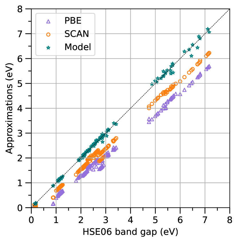
Figure 3: Scatterplot of the band gaps predicted with PBE, SCAN, and a model (Model-4 in TABLE 4) shown alongside the HSE06 values. For PBE and SCAN, we have plotted band gaps of 15 polytypes shown in FIG. 1 for the 15 compositions: C, Si, Ge, SiC, GeC, GeSi, BN, BP, BAs, AlN, AlP, AlAs, GaN, GaP, and GaAs For Model-4, we have shown results for the 7- and 8-bilayered polytypes not used in the construction of the model.

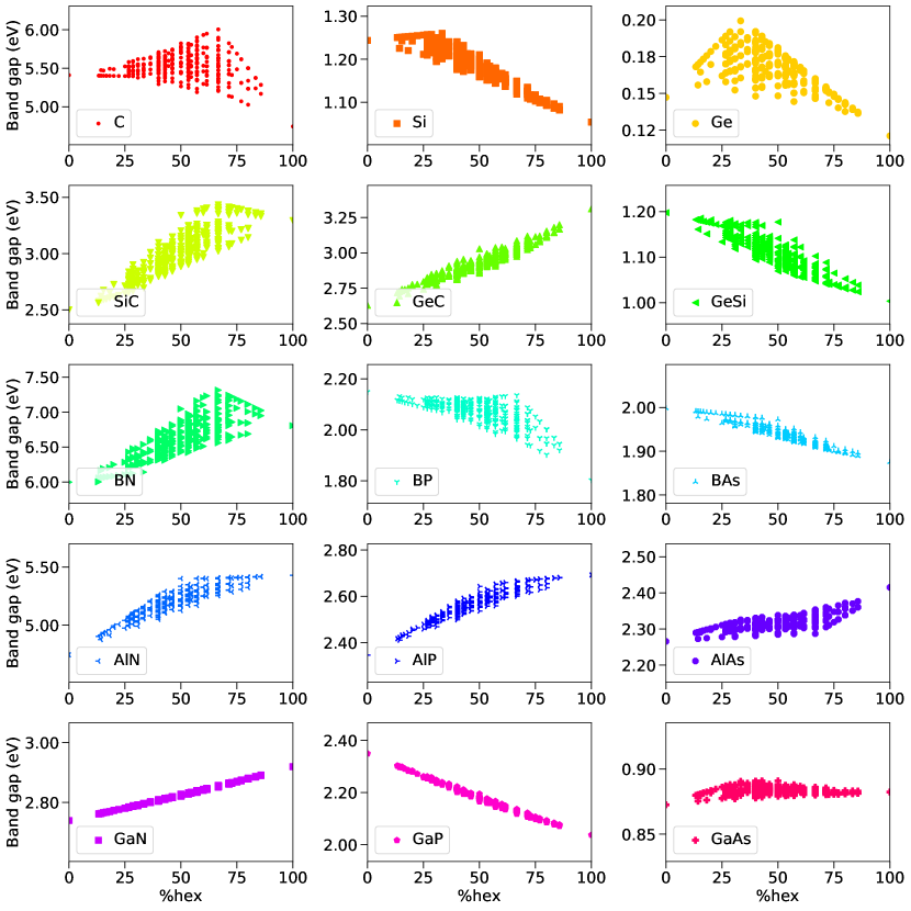
Figure 4: Model-predicted band gaps of 497 polytypes with up to 15 layers in the unit cell. For various compositions, band gaps are plotted along with the percentage hexagonality (%hex) of the crystal structure. Extreme values of %hex corresponds to 3$C$ (%hex = 0) and 2$H$ (%hex = 100) polytypes.

III.3 Accuracy of the best model

The pseudo-spin model (Model-4) developed using $\varepsilon_{g}$ of small polytypes with up to 6 bilayers in the unit cell, models the $\varepsilon_{g}$ of 7- and 8-bilayered polytypes not used in the construction of the model very efficiently, resulting in prediction errors centred around zero. FIG. 3 displays a scatterplot comparing the predictions of Model-4 and the semi-local DFT methods with HSE06 values. The corresponding error metrics are listed in TABLE 6 for a quantitative understanding of the methods’ performances.

GGA-PBE and mGGA-SCAN methods tend to underestimate the HSE06 values on an average by 0.84 and 0.53 eV, respectively. However, the agreement between their predictions and that of HSE06 shows a systematic linearity as indicated by their corresponding $R^{2}$ values greater than 0.99. This trend suggests that a linear adjustment of PBE and SCAN values can agree well with the HSE06 predictions. The corresponding slope and intercept can calibrate PBE/SCAN values for new predictions. However, our study does not delve into a linear correction for PBE or SCAN because our primary focus is exploring long-period polytypes with multiple atoms in the unit cell. In this context, the pseudo-spin models fitted directly to HSE06 reference values will enable rapid application.

For all five error metrics considered in TABLE 6, Model-4 delivers better performances than PBE and SCAN. The MAD for the model’s prediction is about 0.04 eV with an RMSD of about 0.07 eV. These errors are smaller than those of the reference DFT method, HSE06. It is important to note that when applied to other material classes, the DFT methods will retain their transferability with similar errors as seen for the AB polytypes. On the other hand, the models are fitted for a given composition and chemical formula. Hence, even though the pseudo-spin models are very accurate for the polytypes of a given composition, AB, they lose their prediction power when applied to a new composition, such as A₂B. For a given composition, the Ising-type additivity model based on the parameters given in TABLE 5 allows for rapid and accurate estimations of $\varepsilon_{g}$ of long-period polytypes with multiple bilayers in the unit cell.

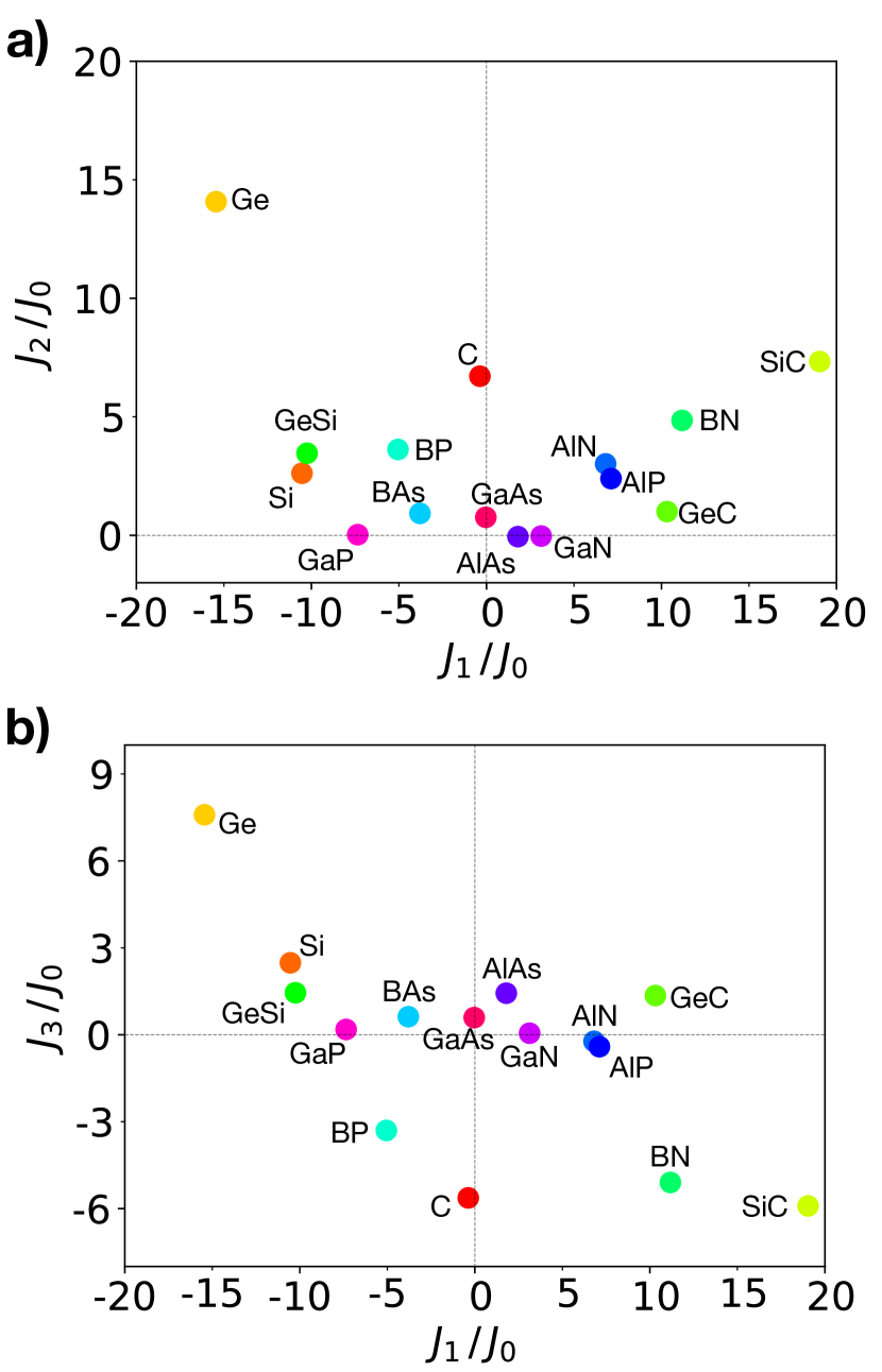
Figure 5: Parameter map for the band gap model of semiconductors: a) Normalized values of $J_{2}$ and $J_{1}$ are plotted. Values on the right (left) side of the plot show an overall increase (decrease) in the band gap with hexagonality of the crystal structure. b) Normalized values of $J_{3}$ and $J_{1}$ are plotted. Values on the right side show a maximum for %hex$>50$, while those on the left side show a maximum for %hex$<50$. For clarity, both axes are multiplied by 100.

Table 6: Error metrics for various approximations corresponding to the plot shown in FIG. 3. MAE, RMSD, MAX (all in eV) correspond to mean absolute error, root mean square deviation and maximum absolute error, respectively. $R^{2}$ and $\rho$ (both dimensionless) correspond to coefficient of determination and Spearman’s rank correlation coefficient, respectively.

Method	MAE	RMSD	MAX	$R^{2}$	$\rho$
PBE	0.841	0.334	1.474	0.996	0.986
SCAN	0.528	0.223	0.947	0.997	0.986
Model	0.039	0.069	0.348	0.999	0.997

III.4 Correlation between band gap and hexagonality

FIG. 4 presents scatterplots depicting the variation in $\varepsilon_{g}$ as a function of %hex for 497 polytypes with up to 15 bilayers. While Model-3 demonstrates improved accuracy for element C (as shown in TABLE4), we employ Model-4 uniformly for all compositions to ensure a fair comparison.

As noted by Choyke et al.Choyke et al. (1964), the experimental band gaps of different phases of SiC, namely 2$H$ (3.33 eV), 3$C$ (2.39 eV), 4$H$ (3.26 eV), and 6$H$ (3.02 eV), show an increasing trend from %hex=0 (3$C$) to %hex=50 (4$H$), and then remain relatively constant for %hex values between 50 and 100. This observation has been further discussed by othersPresser and Nickel (2008); Käckell et al. (1994); Wenzien et al. (1995). Additionally, we have found 8$H$(2)-SiC with %hex=25 exhibits a band gap of 2.80 eV following this trend. FIG. 4 illustrates the relationship between the structure and properties of 497 SiC polytypes. The inclusion of a large number of polytypes in this study offers examples with %hex greater than 50, indicating that the upper bound for $\varepsilon_{g}$ continues to increase until %hex=66.67, after which it gradually declines until reaching %hex=100.

An explanation of the statistical trends seen in FIG. 4 can be deduced by the correlations: $J_{2}$-vs.-$J_{1}$ and $J_{3}$-vs.-$J_{1}$ as depicted in FIG. 5. Since the band gaps of materials are clustered around different mean values, in order to treat all materials on the same footing, we have divided $J_{1-3}$ by $J_{0}$ in this plot. All materials in a particular region on the configuration map exhibit similar behavior. This analysis effectively elucidates the band gap variation with respect to %hex while also providing insights into the existence of polytypes with maximum band gaps for structures with less than or greater than 50% hexagonality.

The band gap behavior of the C polytypes, in terms of %hex, resembles the polytypes of BP (refer to FIG. 4). However, carefully examining the parameters presented in TABLE 5 reveals C and GaAs as exceptions with significantly smaller $J_{1}$ than $J_{2}$ and $J_{3}$. Consequently, C occupies a similar position to GaAs in FIG. 5. Moreover, TABLE 4 highlights that Model-3 outperforms Model-4 for the polytypes of C. Hence, a more robust rationale could have been established by employing the best model for each composition. However, since this study aims to emphasize the applicability of the pseudo-spin model of band gaps for long-period polytypes of SiC, we have refrained from conducting a separate analysis for C polytypes with Model-3.

Furthermore, the relationship between $\varepsilon_{g}$ and %hex has not been extensively discussed for several binary semiconductors. Our findings, as illustrated in FIG. 4, reveal consistent patterns in $\varepsilon_{g}$ for GaN and GaP, albeit with distinct behaviors. Specifically, GaN demonstrates an increase in the bandgap with %hex, while GaP exhibits a reversal of this trend.

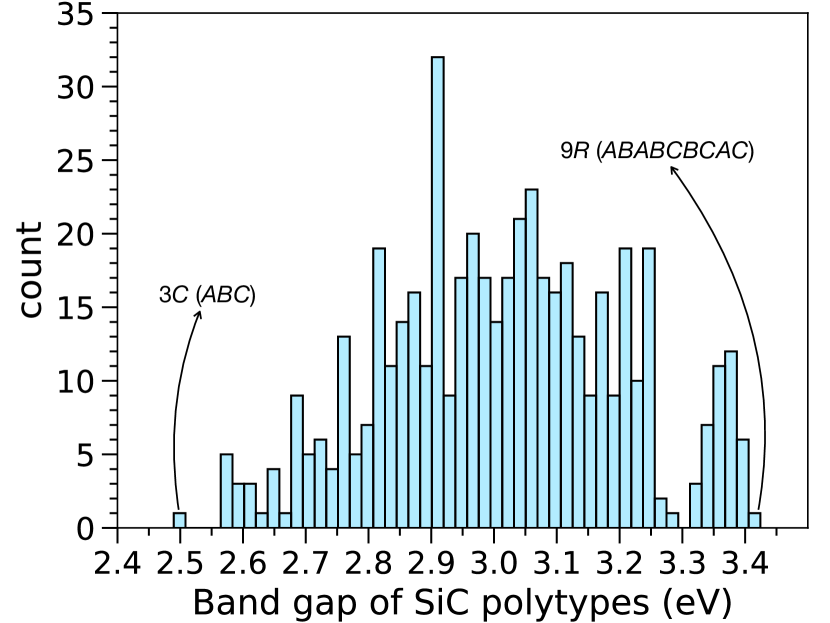
Figure 6: Histogram of model-estimated band gaps of 497 polytypes of SiC with up to 15 bilayers in the unit cell.

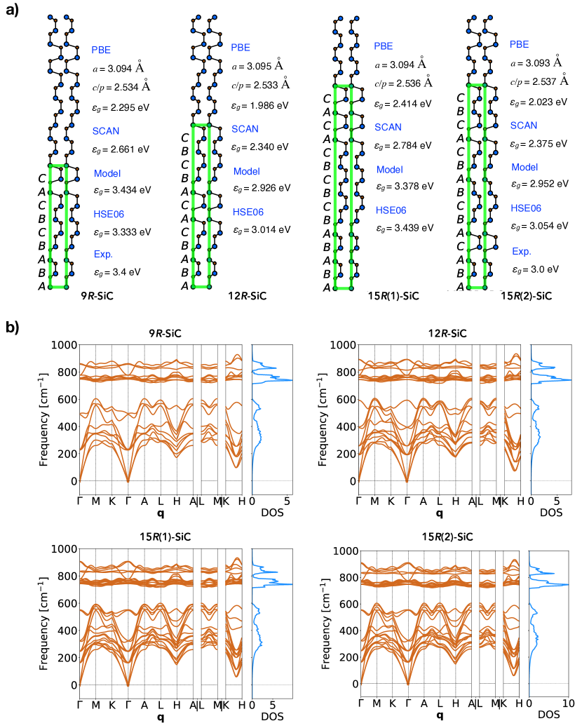
Figure 7: Details of four rhombohedral long-period polytypes of SiC: 9$R$, 12$R$, 15$R$(1), and 15$R$(2): a) Schematic representation of the stacking sequence (brown/blue circles correspond to C/Si atoms), calculated values of lattice parameters and band gaps are given along with available experimental band gapsYaghoubi et al. (2018). b) GGA-PBE phonon band structures along with the corresponding density of states.

Notably, GaAs maintains a relatively constant value of $\varepsilon_{g}$ for all %hex. This trend can be understood through the vanishing interaction parameters $J_{1-3}$ and $K$ listed in TABLE 5. Nevertheless, the structure and cohesive energies of the polytypes of GaAs have been shown to vary with %hexPanse et al. (2011). Furthermore, zero-Kelvin experimental band gaps Kusch et al. (2012) of 2$H$ (1.46 eV) and 3$C$ (1.52 eV) imply a small variation with %hex. In III.1, we discussed how the HSE06 band gap of 3$C$-GaAs widens to 1.14 eV when using the crystal structure determined with HSE06. We also performed separate geometry relaxation of 2$H$-GaAs at the HSE06 level, resulting in $a=4.013$ Å and $c/p=3.307$ Å (see Table S1 for the corresponding PBE values). At this geometry, the HSE06 $\varepsilon_{g}$ of 2$H$-GaAs turned out to be 1.13 eV, differing from the 3$C$ value by only 0.1 eV. For a given polytype of GaAs, DFT-predicted band gaps are sensitive to small changes in lattice parameters. However, across polytypes, they show less variation, resulting in a rather flat profile seen in FIG. 4; see also the almost constant values of the band gaps of GaAs at PBE, SCAN and HSE06 levels in TABLE 3. It is interesting to note that two past studiesZanolli et al. (2007); Giorgi et al. (2020) have noted that many-body effects in the wavefunction are necessary to break the ‘degeneracy’ of $\varepsilon_{g}$ among the wurtzite and zincblende phases of GaAs. In the more recent studyGiorgi et al. (2020), the many-body method G₀W₀ was applied to predict the band gaps of 2$H$- and 3$C$-GaAs as 1.46 and 1.66 eV, in good qualitative and quantitative agreement with the experimental values: 1.46 and 1.52 eVKusch et al. (2012). Hence, even though GaAs is not known to exhibit extensive polytypism as SiC, for the pseudo-spin models to forecast a quantitative trend across hypothetical polytypic phases, it is necessary to consider reference band gaps calculated using post-DFT methods.

III.5 Case study of rhombohedral SiC

Over 250 different polytypes of SiC have been observed in experimental studiesKrishna and Verma (1966). Among them are long-period polytypes containing even more than 50 bilayers in the unit cell, as well as ultralong period polytypes, such as 393$R$ and 594$R$Krishna and Verma (1966); Fal’kovskii and Camassel (1999). While ZnS also exhibits polytypism, it is a direct band gap semiconductor, implying that the variation of $\varepsilon_{g}$ across its polytypic forms is relatively limited. Since SiC is an indirect gap material, it can exhibit diverse gaps due to band-folding effectsLambrecht et al. (1997) across polytypes of different unit cell sizes. FIG. 6 illustrates a histogram depicting the model-predicted $\varepsilon_{g}$ for 497 polytypes of SiC, demonstrating a range of $\approx$0.9 eV. According to the model, the polytype with the smallest $\varepsilon_{g}$ is 3$C$, while the largest gap is found in 9$R$. A past studyYaghoubi et al. (2018) has reported the HSE06 level band gap of this phase to be 3.233 eV and discussed its dynamic stability through phonon analysis. It is worth noting that several long-period polytypes of SiC observed experimentally exhibit rhombohedral symmetry. Those with experimental band gaps are: 9$R$ (%hex=66.67, 3.4 eV)Yaghoubi et al. (2018), 15$R$ (%hex=40, 3.0 eV)Yaghoubi et al. (2018), 21$R$ (%hex=28.57, 2.86 eV)Choyke et al. (1964), and 33$R$ (%hex=36, 3.01 eV)Choyke et al. (1964).

Given the prevalence of polytypes with rhombohedral symmetry in reported studies, we have specifically chosen four phases: 9$R$, 12$R$, and two 15$R$ phases from the 497 set for detailed analysis. Only 4 out of 497 polytypes with $\leq 15$ bilayers are rhombohedral, which highlights the relatively low statistical likelihood of encountering $R$ phases compared to $H$ and $T$. The reason behind the low occurrence of an $R$-polytype is that the unit cell must consist of a multiple of three bilayers with an equal number of $A$, $B$, and $C$-type bilayers. Consequently, although the number of polytypes increases significantly with the number of bilayers in the unit cell, rhombohedral phases represent a tiny fraction within the overall landscape of polytype compounds.

We have optimized the structure of four $R$-type polytypes of silicon carbide (SiC), as depicted in FIG. 7a. We have confirmed that all four phases are dynamically stable by phonon band structure analysis (see FIG. 7b). The stacking sequences, as indicated in List S1 of the SI, reveal the hexagonal stacking percentages (%hex) of each polytype: 66.67% for 9$R$, 50.0% for 12$R$, 80.0% for 15$R$(1), and 40.0% for 15$R$(2). Notably, since the 15$R$(1)-SiC phase exhibits a greater %hex than the 9$R$ phase, comparing their respective band gaps through HSE06 calculations is intriguing. While our model predicts a larger $\varepsilon_{g}$ of 3.43 eV for the 9$R$ polytype, the HSE06 reference method suggests that 15$R$(1) possesses a slightly larger band gap than 9$R$. It is important to acknowledge that a minor discrepancy between the model and HSE06 is expected, considering the average error of the model, as reported in TABLE 4.

Among the various polytypes of SiC, 9$R$, 12$R$, and 15$R$(2) have been experimentally studied. As of yet, the 15$R$(1) polytype has only been investigated computationallyLimpijumnong and Lambrecht (1998). Hence, to gain further insights, we examined the cohesive energies of all four $R$-SiC polytypes using the HSE06 level of theory. Compared to 3$C$-SiC (-7.056344 eV/atom), 2$H$, 9$R$, 12$R$, and 15$R$(1) are higher in energy by 2.11, 0.29, 0.14, and 1.03 meV/atom, respectively. On the other hand, 4$H$ and 15$R$(2) are lower in energy by -0.77 and -0.69 meV/atom, respectively. These findings support previous conclusionsLimpijumnong and Lambrecht (1998) that 15$R$(1) is thermodynamically less stable than 9$R$, yet more stable than the 2$H$ phase. Overall, 15$R$(1) can be regarded as a wide-gap metastable phase of SiC.

Table 7: Energies of the highest valence (V) and the lowest conduction (C) bands of polytypes of SiC used in the model. For each energy, parameters fitted to Eq. 4 are given. In all cases, VBM is at the $\Gamma$-point that is set to zero. All values are in eV.

${\bf k}$		band	Polytypes					Parameters
			2$H$	3$C$	4$H$	5$T$	6$T$		$J_{0}$	$J_{1}$	$J_{2}$	$J_{3}$	$K$
$\Gamma$	(0,0,0)	V	0.000	0.000	0.000	0.000	0.000		0.000	0.000	0.000	0.000	0.000
		C	5.851	6.779	6.154	6.152	6.011		6.115	-0.407	-0.081	-0.057	-0.120
$M$	(1/2,0,0)	V	-1.317	-1.900	-1.233	-1.505	-1.264		-1.413	0.280	0.188	0.012	0.007
		C	3.779	2.341	3.227	2.927	3.388		3.108	0.720	0.084	-0.001	-0.035
$K$	(1/3,1/3,0)	V	-4.115	-2.355	-1.823	-2.567	-2.288		-2.575	-0.385	0.706	-0.494	-0.046
		C	3.294	4.913	5.063	4.020	4.093		4.190	-0.986	0.480	0.177	-0.393
$A$	(0,0,1/2)	V	-0.786	-0.357	-0.226	-0.108	-0.083		-0.222	0.104	0.173	-0.318	0.176
		C	7.004	6.507	6.374	6.129	6.052		6.299	-0.284	-0.191	0.533	-0.265
$L$	(1/2,0,1/2)	V	-2.527	-1.155	-1.690	-1.224	-1.465		-1.504	-0.192	0.075	-0.494	0.262
		C	4.316	3.765	3.650	2.733	3.285		3.160	0.080	-0.195	0.195	-0.685
$H$	(1/3,1/3,1/2)	V	-1.898	-3.320	-2.640	-2.130	-1.852		-2.228	1.126	-0.015	-0.415	0.396
		C	6.163	6.288	4.299	4.465	3.813		4.635	-1.096	-0.963	1.034	-0.627

III.6 Model for band energies at high-symmetry points of the Brillouin zone

The distinct variation in the band gap across different polytypes of SiC is attributed to the indirect nature of their band gapVan Haeringen et al. (1997). Within the band structure, certain high-symmetry points, namely $\Gamma$, $M$, and $K$, represent the band origin with respect to $k_{z}$ (with $k_{z}=0$), while $A$, $L$, and $H$ denote the corresponding band edges (with $k_{z}=1/2$). Across all polytypes examined in this study, the VBM is consistently associated with the downward progression of the $p$-band from $\Gamma$. Only in 2$H$-SiC does the CBM occur at $K$, while in all other polytypes analyzed, the CBM of SiC resides either at $M$ or $L$. Previous studies investigating 2$H$, 3$C$, 4$H$, and 6$H$-SiC have demonstrated that the band gap widens when hexagonality increases from 0 to 50, then remains constant until 100% hexagonality (as in 2$H$), while the CBM energies vary linearly with the hexagonality of the crystal structurePark et al. (1994).

In FIG 8, we present the computed energies of the CB at various high-symmetry $k$-points for different crystal structures of SiC, explicitly focusing on the 15 simplest polytypes. The purpose of this figure is to observe how the hexagonality of the crystal structure influences the CB energy. The plot reveals linear trends suggesting a preference for CBM at $M$ or $L$ for hexagonality less than 90%; beyond this limit, $K$ is a preferred location for CBM. Among the polytypes with up to 15 bilayers, only 2$H$ has %hex$>90$. Other close examples include three 12-bilayer polytypes (12$T$: ABABABABABAC, 12$T$: ABABABABACAC, and 12$H$: ABABABACACAC) with a hexagonality of 83.33% and three 14-bilayer polytypes (14$T$: ABABABABABABAC, 14$T$: ABABABABABACAC, and 14$T$: ABABABABACACAC) with a hexagonality of 85.71. For a comprehensive list of 497 polytypes with up to 15 bilayers in the unit cell, please refer to List S1 in the SI. Among $M$ and $L$ points, the preference for the CBM is not as pronounced. It is expected that in long-period polytypes, the energies of both points would be similar because of band-folding effects. In other words, as the unit cell size increases, the VB and CB along the paths $\Gamma\rightarrow A$, $M\rightarrow L$, and $K\rightarrow H$ tend to exhibit flatter energy profiles with diminishing band dispersions.

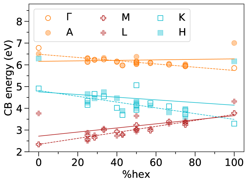
Figure 8: Variation of HSE06 conduction band (CB) energies (in eV) of 15 SiC polytypes (listed in TABLE 1) with the percentage hexagonality (%hex) of the crystal structure. Fitted straight lines are also shown; dashed lines correspond to $\Gamma$, $M$, and $K$ while solid lines correspond to $A$, $L$, and $H$.

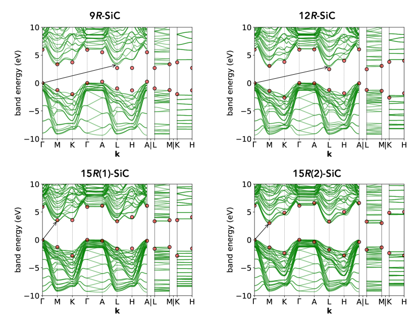
Figure 9: HSE06 electronic band structures of the rhombohedral phases of SiC along with VB and CB energies at the high-symmetry points predicted with a model (red points). The arrow indicates the indirect band gap. In all cases, VBM is set to zero.

PBE, SCAN, and HSE06 band structures of the smallest six polytypes are collected in Figures S1 of SI. It is evident that the underestimation of the band gap is prominent in PBE and SCAN, as observed through the trend: PBE $<$ SCAN $<$ HSE06. Using HSE06 band structures of the 2$H$, 3$C$, 4$H$, 5$T$, and 6$T$ polytypes of SiC, we fitted Model-4 using the energies of VB and CB at each high-symmetry point within the Brillouin zone. The energies and the resulting parameters are provided in TABLE 7. As expected, the model reproduces the target energies for the polytypes used in the model, as illustrated in Figures S2–S6 in the SI.

Additionally, we made predictions for the VB and CB energies at the high-symmetry points for the 6$H$ phase and for phases with 7 and 8 bilayers in the unit cell not included in the model. The SI presents the HSE06 band structures alongside the energies predicted by the model (Figures S7–S16 in the SI). Overall, the predictions align well with HSE06 for all phases, capturing the indirect band gap nature and the associated symmetry of the CBM. However, the model exhibits discrepancies at the $H$ point for a few polytypes. Notably, the model spuriously widens the gap at $H$ consistently by: (i) overestimating the energy of CB and underestimating the VB energy in 6$H$, 7$T$(3) (ii) overestimating the energy of CB with no effect on the corresponding VB in 7$T$(1), 8$T$(1), 8$T$(2), 8$T$(3), and 8$H$(2). In contrast, the gap is underestimated at $H$ in 7$T$(2) and 8$H$(1) (Figure S9 and Figure S12 in the SI). 8$T$(4) is the only case where the model fully agrees with the reference theory, HSE06 (Figure S15 in the SI). Overall, these trends do not indicate the model’s prediction accuracy at the $H$-point to correlate with change in %hex of these polytypes collected in TABLE 1.

To explore the scope to apply the model to predict the positions of the VBM and CBM of long-period polytypes, we applied the models to 9, 12, and 15 $R$ polytypes of SiC. The results are presented in FIG 9. The model’s prediction is overall in good agreement for all four polytypes. The best prediction is seen for 12$R$-SiC with %hex=50. For 15$R$(1) and 15$R$(2), the VB energies are underestimated at $K$ and $H$, respectively. Since 15$R$(1) has %hex=80, the HSE06 CB energy at $H$ is lowered compared to $L$ or $M$ than in 15$R$(2) with %hex=40 as expected according to the linear trends revealed in FIG. 8. In the case of 9$R$-SiC with %hex=66.67, the model significantly underestimates the CB energy at $H$, bringing the energy close to that of $L$ (see FIG 9). This prediction is in disagreement with the linear relationships established using HSE06 band structures shown in FIG. 8 according to which the energies of $K$/$H$ pairs should lie above the energy of $M$/$L$ pairs for %hex$<90$.

In contrast to cohesive energy and the overall band gap, which are size-intensive material properties, the band energies at specific high-symmetry points may be considered size-extensive. In systems with larger unit cell sizes, the energy at high-symmetry points approaches $\Gamma$. Therefore, when building models, it might be helpful to consider the effects of Brillouin zone folding in the band structure for polytypes of different unit cell sizes.

IV Computational Details

IV.1 Crystal structure generation

For all polytypes, in four crystal classes—$C$, $H$, $T$, and $R$—we generated initial structures in a hexagonal lattice defined by the lattice vectors:

$${\bf a}_{1} = \hat{x}a/2-\hat{y}\sqrt{3}a/2$$

$${\bf a}_{2} = \hat{x}a/2+\hat{y}\sqrt{3}a/2$$

$${\bf a}_{3} = \hat{z}c$$

Notably, the cubic polytype 3$C$ is a specific case of $R$ when the angles $\alpha$, $\beta$, and $\gamma$ are equal to $60^{\circ}$, along with the condition $a=b=c$ that usually applies to $R$ systems. The fractional coordinates for a given polytype are generated as follows:

1. For the $A$, $B$, and $C$ type bilayers, the $x$ and $y$ Wyckoff coordinates (coefficients of ${\bf a}_{1}$ and ${\bf a}_{2}$ lattice vectors) are $\left(0,0\right)$, $\left(\frac{1}{3},\frac{2}{3}\right)$, and $\left(\frac{2}{3},\frac{1}{3}\right)$, respectively.

2. The $z$-coordinate of atom-1 (e.g., Si in SiC) is assigned as $q/p+u_{i}$, where $p$ represents the total number of bilayers, $q$ ranges from $0$ to $p-1$, and $u_{i}$ is a free parameter for atom-1 in bilayer $i$.

3. For atom-2 (e.g., C in SiC), the $z$-coordinate is assigned as $q/p+d+v_{i}$, where $d=\frac{3}{4q}$ represents an increment in the $z$-direction, and $v_{i}$ is a free parameter for atom-2 in bilayer $i$.

Similar structural information are available in  Refs.66; 76.

IV.2 Density functional theory calculations

Lattice vectors and atomic coordinates were fully relaxed with the all-electron, numeric atom-centred orbital (NAO) code FHI-aimsBlum et al. (2009) with the Perdew–Burke–Ernzerhof (PBE)Perdew et al. (1996b) GGA XC functional. In all calculations a tight basis set was employed. The quality of the NAO basis sets used in this study can be assessed by comparing them with the $E_{\rm cut}$ parameter in the plane-wave framework. For determining the energies of 63 binary materials, the accuracy of light and tight basis sets were shown to be equivalent to that of using an $E_{\rm cut}$ of 400 eV and 800 eV in the plane-wave frameworkCarbogno et al. (2022). During geometry relaxations, the convergence thresholds for electron density, analytic gradients, and maximum force component for gradient-based minimization were set to $10^{-6}$ $e/$ų (where $e$ is the charge of an electron), $5\times 10^{-4}$ eV/Å, and $5\times 10^{-3}$ eV/Å, respectively. Lattice relaxations were performed using FHI-aims’ feature to constrain the crystal structure at the desired space group and to constrain the coordinates of the atoms to fixed forms corresponding to the Wyckoff sites of interestLenz et al. (2019); Lenz-Himmer (2022). Using this approach, it is possible to symbolically map the deviations in the $z$ Wyckoff coordinates from their ideal positions and to explicitly determine the corrections $u_{i}$ and $v_{i}$ mentioned in IV.1.

The crystal structures of the 2$H$ phase were optimized for all compositions, and the corresponding lattice constant $a$ was used as the initial guess for polytypes with larger unit cells. Further, we used $p\times c^{2H}/2$, where $c^{2H}$ is the minimum energy value of the $c$-lattice constant of the 2$H$ polytype, for other polytypes with $p$ bilayers. All lattice parameters reported here are calculated at the GGA-PBE level. We report band gaps calculated using PBE geometries at three levels: GGA-PBE, the strongly constrained and appropriately normed (SCAN) mGGA functional Sun et al. (2015) and the Heyd–Scuseria–Ernzerhof (HSE)Krukau et al. (2006) hybrid XC functional with a screening parameter of $\omega=0.11$ bohr^-1 (referred to as the HSE06 functional).

For each reciprocal lattice vector (${\bf b}_{i}$, where $i$ = 1, 2, 3), $k$-grids were selected as equally spaced points between $-\pi|{\bf b}_{i}|$ and $+\pi|{\bf b}_{i}|+dk$, with a separation (or $k$-spacking) of $dk$ (in Å^-1). An additional $dk$ value was added to the upper limit to ensure a symmetric range, as $\pi|{\bf b}_{i}|$ may not be divisible by $dk$. The $k$-grids size obtained in this manner is directly linked to the unit cell volume, which is determined by the real-space lattice vectors (${\bf a}_{i}$). Accordingly, larger volumes result in a smaller number of $k$-grids. In our calculations, we used $dk=0.3$ Å^-1 and sampled the Brillouin zone using the Monkhorst–Pack schemeMonkhorst and Pack (1976). For 2$H$-SiC phase, the number of $k$-grids is $9\times 9\times 6$ while for 3$C$-SiC and 4$H$-SiC, the number of $k$-grids is $9\times 9\times 4$. For SiC polytypes with 5-8 bilayers, $9\times 9\times 3$ $k$-grids were used to sample the Brillouin zone. In the case of long-period polytypes of SiC—9$R$, 12$R$, 15$R$(1), and 15$R$(2)—our approach yielded initial $k$-grids of size $9\times 9\times 2$, which were subsequently increased to $9\times 9\times 3$ in order to improve the band structures.

Phonon spectra were obtained for supercells using finite-derivatives of analytic forces with an atomic displacement of 0.01 Å and tighter thresholds ($10^{-7}$ $e/$ų for electron density and $10^{-6}$ eV/Å for analytic forces) using the Phonopy codeTogo and Tanaka (2015) interfaced with FHI-aims. For 9$R$, 12$R$, 15$R$(1), and 15$R$(2), we used a $3\times 3\times 1$ supercell containing 162, 216, 270, and 270 atoms, respectively. Scalar relativistic effects are accounted for within the atomic zeroth-order regular approximation (atomic ZORA)Blum et al. (2009). All band structures were generated along high-symmetry points in the Brillouin zone as defined by Setyawan et al.Setyawan and Curtarolo (2010). Optimized crystal structures were visually analyzed using the program VestaMomma and Izumi (2011).

V Conclusions

We have conducted a systematic study on the polytypes of group IV elements, binary compounds of IV-IV and III-V groups, and employed hybrid-DFT level calculations to model their band gaps. Our approach, inspired by the cluster expansion of the Ising model, incorporates a four-body coupling that results in an overall error of 0.039 eV across the investigated compositions. Remarkably, the model’s predictions exhibit minimal systematic errors, aligning well with the HSE06 level band gaps for long-period polytypes not used during the model’s development. The mean absolute deviation of our model is an order of magnitude smaller than that of GGA-PBE and mGGA-SCAN DFT methods.

The accuracy of our model enables us to efficiently determine the band gaps of 497 polytypes for each composition containing up to 15 bilayers in the unit cell. Although GGA/mGGA band gaps calibrated using linear fitting could demonstrate better agreement with hybrid-DFT values, implementing such methods necessitates calculating GGA/mGGA band structure, increasing the computational overhead. Therefore, empirical models reported in this study offer a practical solution for the rapid high-throughput screening of electronic properties in the materials space of polytypes.

We re-examined the empirical relationship between hexagonality and band gap in SiC polytypes and observed that the highest band gaps occur for hexagonality greater than 50%. We have also established similar correlations for the other compositions: BN, BP, AlN, and AlP. Using a phase-diagram-type analysis based on the model parameters, we have predicted the statistical dependence of band gaps on the hexagonality of the crystal structure. We focussed on SiC polytypes and identified a metastable rhombohedral phase, 15$R$(1), with a higher band gap (3.44 eV at the HSE06 level) than the previously studied 9$R$ phase.

Furthermore, we have explored the feasibility of modeling band gaps at high-symmetry points of the Brillouin zone. While these models exhibit minimal errors for the overall band gap, their accuracy diminishes when predicting individual band energies at high-symmetry points. For long-period polytypes, one expects the bands connecting the band origins ($\Gamma$/$M$/$K$) and their corresponding edges ($A$/$L$/$H$) to be flat. Since our models use the information from small polytypes, significant disparities between the band origins and edges arise when applied to larger polytypes. On the other hand, for the total band gaps, the additivity model presented here delivers better accuracies than that of the reference DFT method. Hence, empirical models applied in this study can be employed fruitfully using more precise reference band gaps that incorporate effects such as many-body correlation or spin-orbit coupling.

VI Data Availability

The data that support the findings of this study are within the article and its supplementary material. Lattice parameters, electronic band structures, and stacking sequences are provided.

VII Acknowledgments

SJ gratefully acknowledges a summer fellowship of the TIFR Visiting Students’ Research Programme (VSRP). We acknowledge the support of the Department of Atomic Energy, Government of India, under Project Identification No. RTI 4007. All calculations have been performed using the Helios computer cluster, which is an integral part of the MolDis Big Data facility, TIFR Hyderabad (http://moldis.tifrh.res.in).

VIII Author Declarations

VIII.1 Author contributions

RR: Conceptualization; Funding acquisition; Project administration and supervision; Resources; Data collection and analysis; Writing (main). SJ: Preliminary investigation; Analysis; Writing (supporting).

VIII.2 Conflicts of Interest

The authors have no conflicts of interest to disclose.

References

- Perdew et al. (2017) J. P. Perdew, W. Yang, K. Burke, Z. Yang, E. K. Gross, M. Scheffler, G. E. Scuseria, T. M. Henderson, I. Y. Zhang, A. Ruzsinszky, et al., Proc. Natl. Acad. Sci. USA 114, 2801 (2017), URL https://doi.org/10.1073/pnas.1621352114.
- Perdew and Levy (1983) J. P. Perdew and M. Levy, Phys. Rev. Lett. 51, 1884 (1983), URL https://doi.org/10.1103/PhysRevLett.51.1884.
- Perdew and Ruzsinszky (2018) J. P. Perdew and A. Ruzsinszky, Eur. Phys. J. B 91, 1 (2018), URL https://doi.org/10.1140/epjb/e2018-90083-y.
- Perdew and Ruzsinszky (2010) J. P. Perdew and A. Ruzsinszky, Int. J. Quantum Chem. 110, 2801 (2010), URL https://doi.org/10.1002/qua.22829.
- Perdew et al. (2009) J. P. Perdew, A. Ruzsinszky, L. A. Constantin, J. Sun, and G. I. Csonka, J. Chem. Theory Comput. 5, 902 (2009), URL https://doi.org/10.1021/ct800531s.
- Mizokawa and Fujimori (1996) T. Mizokawa and A. Fujimori, Phys. Rev. B 54, 5368 (1996), URL https://doi.org/10.1103/PhysRevB.54.5368.
- Heyd et al. (2003) J. Heyd, G. E. Scuseria, and M. Ernzerhof, J. Chem. Phys. 118, 8207 (2003), URL https://doi.org/10.1063/1.1564060.
- Krukau et al. (2006) A. V. Krukau, O. A. Vydrov, A. F. Izmaylov, and G. E. Scuseria, J. Chem. Phys. 125, 224106 (2006), URL https://doi.org/10.1063/1.2404663.
- Perdew et al. (1996a) J. P. Perdew, M. Ernzerhof, and K. Burke, J. Chem. Phys. 105, 9982 (1996a), URL https://doi.org/10.1063/1.472933.
- Chan and Ceder (2010) M. K. Chan and G. Ceder, Phys. Rev. Lett. 105, 196403 (2010), URL https://doi.org/10.1103/PhysRevLett.105.196403.
- Verma and Truhlar (2016) P. Verma and D. G. Truhlar, Theor. Chim. Acta 135, 182 (2016), URL https://doi.org/10.1007/s00214-016-1927-4.
- Ramakrishnan et al. (2009) R. Ramakrishnan, A. V. Matveev, and N. Rösch, Chem. Phys. Lett. 468, 158 (2009), URL https://doi.org/10.1016/j.cplett.2008.12.021.
- Kulik (2015) H. J. Kulik, J. Chem. Phys. 142, 240901 (2015), URL https://doi.org/10.1063/1.4922693.
- Morales-García et al. (2017) Á. Morales-García, R. Valero, and F. Illas, J. Phys. Chem. C 121, 18862 (2017), URL https://doi.org/10.1021/acs.jpcc.7b07421.
- Lee et al. (2016) J. Lee, A. Seko, K. Shitara, K. Nakayama, and I. Tanaka, Phys. Rev. B 93, 115104 (2016), URL https://doi.org/10.1103/PhysRevB.93.115104.
- Na et al. (2020) G. S. Na, S. Jang, Y.-L. Lee, and H. Chang, J. Phys. Chem. A 124, 10616 (2020), URL https://doi.org/10.1021/acs.jpca.0c07802.
- Moreno et al. (2021) J. R. Moreno, J. Flick, and A. Georges, Physical Rev. Materials 5, 083802 (2021), URL https://doi.org/10.1103/PhysRevMaterials.5.083802.
- Lentz and Kolpak (2020) L. C. Lentz and A. M. Kolpak, J. Phys.: Condens. Matter 32, 155901 (2020), URL https://doi.org/10.1088/1361-648X/ab5f3a.
- Zhang et al. (2022) L. Zhang, T. Su, M. Li, F. Jia, S. Hu, P. Zhang, and W. Ren, Mater. Today Commun. 33, 104630 (2022), URL https://doi.org/10.1016/j.mtcomm.2022.104630.
- Ramakrishnan et al. (2015) R. Ramakrishnan, P. O. Dral, M. Rupp, and O. A. Von Lilienfeld, J. Chem. Theory Comput. 11, 2087 (2015), URL https://doi.org/10.1021/acs.jctc.5b00099.
- Borlido et al. (2020) P. Borlido, J. Schmidt, A. W. Huran, F. Tran, M. A. Marques, and S. Botti, npj Comput Mater 6, 96 (2020), URL https://doi.org/10.1038/s41524-020-00360-0.
- Wu et al. (2016) Q. Wu, B. He, T. Song, J. Gao, and S. Shi, Comput. Mater. Sci. 125, 243 (2016), URL https://doi.org/10.1016/j.commatsci.2016.08.034.
- Laks et al. (1992) D. B. Laks, L. Ferreira, S. Froyen, and A. Zunger, Phys. Rev. B 46, 12587 (1992), URL https://doi.org/10.1103/PhysRevB.46.12587.
- Elliott (1961) R. J. Elliott, Phys. Rev. 124, 346 (1961), URL https://doi.org/10.1103/PhysRev.124.346.
- Selke (1988) W. Selke, Phys. Rep. 170, 213 (1988), URL https://doi.org/10.1016/0370-1573(88)90140-8.
- Limpijumnong and Lambrecht (1998) S. Limpijumnong and W. R. Lambrecht, Phys. Rev. B 57, 12017 (1998), URL https://doi.org/10.1103/PhysRevB.57.12017.
- Panse et al. (2011) C. Panse, D. Kriegner, and F. Bechstedt, Phys. Rev. B 84, 075217 (2011), URL https://doi.org/10.1103/PhysRevB.84.075217.
- Raffy et al. (2002) C. Raffy, J. Furthmüller, and F. Bechstedt, Phys. Rev. B 66, 075201 (2002), URL https://doi.org/10.1103/PhysRevB.66.075201.
- Moriguchi et al. (2021) K. Moriguchi, T. Miyakawa, S. Ogane, R. Sato, K. Tsutsui, and Y. Tanaka, MRS Advances 6, 163 (2021), URL https://doi.org/10.1557/s43580-021-00044-x.
- Keller et al. (2023) M. Keller, A. Belabbes, J. Furthmüller, F. Bechstedt, and S. Botti, Physical Rev. Materials 7, 064601 (2023), URL https://doi.org/10.1103/PhysRevMaterials.7.064601.
- Kobayashi and Komatsu (2012) K. Kobayashi and S. Komatsu, J. Phys. Soc. Jpn. 81, 024714 (2012), URL https://doi.org/10.1143/JPSJ.81.024714.
- Moriguchi et al. (2013) K. Moriguchi, K. Kamei, K. Kusunoki, N. Yashiro, and N. Okada, ada, N.: J. Mater. Res 28, 7 (2013), URL https://doi.org/10.1557/jmr.2012.206.
- Bechstedt and Belabbes (2013) F. Bechstedt and A. Belabbes, J. Phys.: Condens. Matter 25, 273201 (2013), URL https://doi.org/10.1088/0953-8984/25/27/273201.
- Smith et al. (1984) J. Smith, J. Yeomans, and V. Heine, Modulated Structure Materials pp. 95–105 (1984), URL https://link.springer.com/chapter/10.1007/978-94-009-6195-1_5.
- Trigunayat (1991) G. Trigunayat, Solid state ionics 48, 3 (1991), URL https://doi.org/10.1016/0167-2738(91)90200-U.
- Heine (1985) V. Heine, Computation of Electronic Structure: Its Role in the Development of Solid State Physics (Springer US, Boston, MA, 1985), pp. 1–5, ISBN 978-1-4757-0899-8, URL https://doi.org/10.1007/978-1-4757-0899-8_1.
- Cheng et al. (1989) C. Cheng, R. Needs, V. Heine, and I. Jones, Phase Transitions 16, 263 (1989), URL https://doi.org/10.1080/01411598908245702.
- Cheng et al. (1990) C. Cheng, V. Heine, and I. Jones, J. Phys.: Condens. Matter 2, 5097 (1990), URL https://doi.org/10.1088/0953-8984/2/23/002.
- Kayastha and Ramakrishnan (2021) P. Kayastha and R. Ramakrishnan, J. Chem. Phys. 154, 061102 (2021), URL https://doi.org/10.1063/5.0041717.
- Pallikara et al. (2022) I. Pallikara, P. Kayastha, J. M. Skelton, and L. D. Whalley, Electron. Struct. (2022), URL https://doi.org/10.1088/2516-1075/ac78b3.
- Rohrer (2001) G. S. Rohrer, Structure and bonding in crystalline materials (Cambridge University Press, 2001).
- Tilley (2020) R. J. Tilley, Crystals and crystal structures (John Wiley & Sons, 2020).
- Halac et al. (2002) E. Halac, E. Burgos, and H. Bonadeo, Phys. Rev. B 65, 125202 (2002), URL https://doi.org/10.1103/PhysRevB.65.125202.
- Polya and Read (2012) G. Polya and R. C. Read, Combinatorial enumeration of groups, graphs, and chemical compounds (Springer Science & Business Media, 2012).
- Chakraborty et al. (2019) S. Chakraborty, P. Kayastha, and R. Ramakrishnan, J. Chem. Phys. 150, 114106 (2019), URL https://doi.org/10.1063/1.5088083.
- Douglas and Hollingsworth (2012) B. E. Douglas and C. A. Hollingsworth, Symmetry in bonding and spectra: An introduction (Academic Press, 2012).
- Müller (2013) U. Müller, Symmetry relationships between crystal structures: applications of crystallographic group theory in crystal chemistry, vol. 18 (OUP Oxford, 2013).
- McLarnan (1981) T. McLarnan, Z. Krystallogr. 155, 269 (1981), URL https://doi.org/10.1524/zkri.1981.155.3-4.269.
- Lothaire (1997) M. Lothaire, Combinatorics on words, vol. 17 (Cambridge university press, 1997).
- Guinier et al. (1984) A. Guinier, G. Bokij, K. Boll-Dornberger, J. Cowley, S. Ďurovič, H. Jagodzinski, P. Krishna, P. De Wolff, B. Zvyagin, D. Cox, et al., Acta Cryst. 40, 399 (1984), URL https://doi.org/10.1107/S0108767384000842.
- Ramsdell (1947) L. S. Ramsdell, American Mineralogist 32, 64 (1947), URL https://pubs.geoscienceworld.org/msa/ammin/article-abstract/32/1-2/64/538650/Studies-on-silicon-carbide.
- Ortiz et al. (2013) A. L. Ortiz, F. Sánchez-Bajo, F. L. Cumbrera, and F. Guiberteau, J. Appl. Cryst. 46, 242 (2013), URL https://doi.org/10.1107/S0021889812049151.
- Cheng et al. (1988) C. Cheng, R. Needs, and V. Heine, J. Phys. C: Solid State Phys. 21, 1049 (1988), URL https://doi.org/10.1088/0022-3719/21/6/012.
- Price and Yeomans (1984) G. D. Price and J. Yeomans, Acta Cryst. 40, 448 (1984), URL https://doi.org/10.1107/S0108768184002469.
- Plumer et al. (1988) M. Plumer, K. Hood, and A. Caillé, J. Phys. C: Solid State Phys. 21, 4189 (1988), URL https://doi.org/10.1088/0022-3719/21/23/006.
- Gomes de Mesquita (1967) A. d. Gomes de Mesquita, Acta Cryst. 23, 610 (1967), URL https://doi.org/10.1107/S0365110X67003275.
- Bauer et al. (1998) A. Bauer, J. Kräußlich, L. Dressler, P. Kuschnerus, J. Wolf, K. Goetz, P. Käckell, J. Furthmüller, and F. Bechstedt, Phys. Rev. B 57, 2647 (1998), URL https://doi.org/10.1103/PhysRevB.57.2647.
- Yang et al. (2016) Z.-h. Yang, H. Peng, J. Sun, and J. P. Perdew, Phys. Rev. B 93, 205205 (2016), URL https://doi.org/10.1103/PhysRevB.93.205205.
- Heyd et al. (2005) J. Heyd, J. E. Peralta, G. E. Scuseria, and R. L. Martin, J. Chem. Phys. 123, 174101 (2005), URL https://doi.org/10.1063/1.2085170.
- Backes et al. (1994) W. Backes, P. Bobbert, and W. Van Haeringen, Phys. Rev. B 49, 7564 (1994), URL https://doi.org/10.1103/PhysRevB.49.7564.
- Zhuang and Hennig (2012) H. L. Zhuang and R. G. Hennig, Appl. Phys. Lett. 101, 153109 (2012), URL https://doi.org/10.1063/1.4758465.
- Kusch et al. (2012) P. Kusch, S. Breuer, M. Ramsteiner, L. Geelhaar, H. Riechert, and S. Reich, Phys. Rev. B 86, 075317 (2012), URL https://doi.org/10.1103/PhysRevB.86.075317.
- Zhao and Truhlar (2009) Y. Zhao and D. G. Truhlar, J. Chem. Phys. 130, 074103 (2009), URL https://doi.org/10.1063/1.3076922.
- Choyke et al. (1964) W. Choyke, D. Hamilton, and L. Patrick, Phys. Rev. 133, A1163 (1964), URL https://doi.org/10.1103/PhysRev.133.A1163.
- Presser and Nickel (2008) V. Presser and K. G. Nickel, Crit. Rev. Solid State Mater. Sci. 33, 1 (2008), URL https://doi.org/10.1080/10408430701718914.
- Käckell et al. (1994) P. Käckell, B. Wenzien, and F. Bechstedt, Phys. Rev. B 50, 10761 (1994), URL https://doi.org/10.1103/PhysRevB.50.10761.
- Wenzien et al. (1995) B. Wenzien, P. Käckell, F. Bechstedt, and G. Cappellini, Phys. Rev. B 52, 10897 (1995), URL https://doi.org/10.1103/PhysRevB.52.10897.
- Yaghoubi et al. (2018) A. Yaghoubi, R. Singh, and P. Melinon, Cryst. Growth Des. 18, 7059 (2018), URL https://doi.org/10.1021/acs.cgd.8b01218.
- Zanolli et al. (2007) Z. Zanolli, F. Fuchs, J. Furthmüller, U. von Barth, and F. Bechstedt, Phys. Rev. B 75, 245121 (2007), URL https://doi.org/10.1103/PhysRevB.75.245121.
- Giorgi et al. (2020) G. Giorgi, M. Amato, S. Ossicini, X. Cartoixa, E. Canadell, and R. Rurali, J. Phys. Chem. C 124, 27203 (2020), URL https://doi.org/10.1021/acs.jpcc.0c09391.
- Krishna and Verma (1966) P. Krishna and A. R. Verma, Phys. Status Solidi B 17, 437 (1966), URL https://doi.org/10.1002/pssb.19660170202.
- Fal’kovskii and Camassel (1999) L. Fal’kovskii and J. Camassel, Jetp Lett. 69, 268 (1999), URL https://doi.org/10.1134/1.568016.
- Lambrecht et al. (1997) W. R. Lambrecht, S. Limpijumnong, S. Rashkeev, and B. Segall, Phys. Status Solidi B 202, 5 (1997), URL https://doi.org/10.1002/1521-3951(199707)202:1%3C5::AID-PSSB5%3E3.0.CO;2-L.
- Van Haeringen et al. (1997) W. Van Haeringen, P. Bobbert, and W. Backes, Phys. Status Solidi B 202, 63 (1997), URL https://doi.org/10.1002/1521-3951(199707)202:1%3C63::AID-PSSB63%3E3.0.CO;2-E.
- Park et al. (1994) C. Park, B.-H. Cheong, K.-H. Lee, and K.-J. Chang, Phys. Rev. B 49, 4485 (1994), URL https://doi.org/10.1103/PhysRevB.49.4485.
- Bauer et al. (2001) A. Bauer, P. Reischauer, J. Kräusslich, N. Schell, W. Matz, and K. Goetz, Acta Cryst. 57, 60 (2001), URL https://doi.org/10.1107/S0108767300012915.
- Blum et al. (2009) V. Blum, R. Gehrke, F. Hanke, P. Havu, V. Havu, X. Ren, K. Reuter, and M. Scheffler, Comput. Phys. Commun. 180, 2175 (2009), URL https://www.sciencedirect.com/science/article/pii/S0010465509002033.
- Perdew et al. (1996b) J. P. Perdew, K. Burke, and M. Ernzerhof, Phys. Rev. Lett. 77, 3865 (1996b), URL https://doi.org/10.1103/PhysRevLett.77.3865.
- Carbogno et al. (2022) C. Carbogno, K. S. Thygesen, B. Bieniek, C. Draxl, L. M. Ghiringhelli, A. Gulans, O. T. Hofmann, K. W. Jacobsen, S. Lubeck, J. J. Mortensen, et al., npj Comput Mater 8, 1 (2022), URL https://doi.org/10.1038/s41524-022-00744-4.
- Lenz et al. (2019) M.-O. Lenz, T. A. Purcell, D. Hicks, S. Curtarolo, M. Scheffler, and C. Carbogno, npj Comput Mater 5, 1 (2019), URL https://doi.org/10.1038/s41524-019-0254-4.
- Lenz-Himmer (2022) M.-O. Lenz-Himmer, Towards Efficient Novel Materials Discovery (Humboldt-Universität zu Berlin, 2022), URL https://edoc.hu-berlin.de/handle/18452/25237.
- Sun et al. (2015) J. Sun, A. Ruzsinszky, and J. P. Perdew, Phys. Rev. Lett. 115, 036402 (2015), URL https://doi.org/10.1103/PhysRevLett.115.036402.
- Monkhorst and Pack (1976) H. J. Monkhorst and J. D. Pack, Phys. Rev. B 13, 5188 (1976), URL https://doi.org/10.1103/PhysRevB.13.5188.
- Togo and Tanaka (2015) A. Togo and I. Tanaka, 108, 1 (2015), URL https://www.sciencedirect.com/science/article/pii/S1359646215003127.
- Setyawan and Curtarolo (2010) W. Setyawan and S. Curtarolo, Comput. Mater. Sci. 49, 299 (2010), URL https://doi.org/10.1016/j.commatsci.2010.05.010.
- Momma and Izumi (2011) K. Momma and F. Izumi, J. Appl. Cryst. 44, 1272 (2011), URL https://doi.org/10.1107/S0021889811038970.