Blockchain scaling and liquidity concentration on decentralized exchanges

Abstract

Liquidity providers (LPs) on decentralized exchanges (DEXs) can protect themselves from adverse selection risk by updating their positions more frequently. However, repositioning is costly, because LPs have to pay gas fees for each update. We analyze the causal relation between repositioning and liquidity concentration around the market price, using the entry of blockchain scaling solutions, Arbitrum and Polygon, as our instruments. Lower gas fees on scaling solutions allow LPs to update more frequently than on Ethereum. Our results demonstrate that higher repositioning intensity and precision lead to greater liquidity concentration, which benefits small trades by reducing their slippage.

JEL classifications: G14, G18, G19

Keywords: decentralized exchanges, FinTech, gas fees, liquidity concentration, market depth, slippage

1 Introduction

One of the major cryptoasset exchanges, FTX, filed for bankruptcy on November 11, 2022. Crucially, FTX kept custody of its client deposits. Thus, whereas the exact reasons for its collapse were the subject of investigation by the US Securities and Exchange Commission (SEC), at least $1B of its customers’ funds have vanished, according to Reuters. FTX was a centralized exchange (CEX), with all trades taking place through a limit order book (LOB). In any LOB-based market, a central institution, such as FTX, is needed to match trades and keep records of all transactions.

A recent alternative to CEXs are so-called decentralized exchanges (DEXs) that operate directly on the blockchain. In contrast to CEXs, users themselves keep custody of their assets on DEXs. They execute their trades directly from their wallet, using smart contracts, i.e. a set of pre-programmed rules. Therefore, executing directly on the blockchain provides higher level of security for clients’ funds. Indeed, there is evidence of significant trading volume shifting to DEXs in the week of FTX collapse. According to Reuters, “volumes at the largest DEX, Uniswap, spiked to $17.2 billion in the week of Nov 6-13, from just over $6 billion the week before”.

This higher level of security on DEXs comes, however, at a cost. First, transactions are overall slower, since they have to be validated by “miners” or “validators” before being recorded on the blockchain. Second, users of the blockchain have to compensate validators with the so-called “gas fees” for their efforts. Importantly, “gas fees” are paid not only by liquidity demanders, but also by liquidity providers (LPs). Essentially, gas fees represent a fixed cost and act as a “transaction tax” for every transaction added to the blockchain. Liquidity demanders pay gas fees whenever they would like to execute a trade. Liquidity providers pay gas fees whenever they deposit or withdraw liquidity from the exchange.

In this paper, we analyze the effects of repositioning intensity, i.e. frequency of position updates by LPs, on liquidity concentration on the largest DEX, Uniswap v3. Much alike traditional market makers, LPs are subject to adverse selection risk [15, 6, 9]. To protect themselves from being adversely selected, LPs need to update their positions in response to changes in the market price, similar to canceling and reposting limit orders in the LOB. With lower gas fees, it is cheaper for LPs to update their liquidity positions. Consequently, they can reposition more frequently, which results in better protection from adverse selection. With better protection from adverse selection, LPs can earn higher fees (for the same amount of capital deposited) by setting narrower price ranges around the market price, i.e. their positions become more concentrated. Thus, we expect that a higher repositioning intensity by LPs leads to higher concentration of aggregate liquidity around the market price.

In contrast, if gas fees are high, LPs should only update their positions if the market price sufficiently deviates from their position’s price range, as repositioning is costly. Therefore, we expect LPs to set wider price ranges when they are not able to update frequently, in order to reduce adverse selection risk. Lower repositioning intensity should thus result in lower concentration of aggregate liquidity in the pool. Overall, concentration of aggregate pool liquidity around the market price is important, because higher liquidity concentration translates into lower slippage and thus lower execution cost for traders.

Testing the empirical relation between repositioning intensity and liquidity concentration might be problematic, because repositioning intensity is potentially endogenous. A choice of an LP to update their position can in itself depend on the current liquidity concentration in the pool. To identify the causal effect of repositioning intensity, we use the launch of Uniswap v3 on two Ethereum scaling solutions, Arbitrum and Polygon, as our instruments. Blockchain scaling solutions allow for a quicker validation of transactions, with an average block time of 0.25-3 seconds, relative to Ethereum’s 12 seconds. Moreover, scaling solutions charge significantly lower gas fees of only around $0.01 on Polygon and $0.20-$2 on Arbitrum per trade on Uniswap v3, as compared to an average gas fee of $14 on Ethereum. Importantly, lower gas fees on scaling solutions allow LPs to update their positions more frequently. Therefore, we use the launch of Uniswap v3 on scaling solutions as our instrument for an exogenous increase in repositioning intensity of LPs.

We test our predictions above using the two most liquid pairs on Uniswap v3, ETH/USDC 0.05% and ETH/USDC 0.3%, that are traded across all three chains: Ethereum, Arbitrum and Polygon. Hence, our dataset consists of six distinct liquidity pools. Our sample period starts in January 2022, after the launch of Uniswap v3 on both Arbitrum and Polygon, and ends in June 2023.

We first examine trading volume, trade size and total value locked (TVL) in liquidity pools across all chains. Overall, we observe significantly larger trades, volumes and TVL on Ethereum, relative to scaling solutions. These results are largely due to higher security of Ethereum, driven by its high number of validators. In contrast, LPs are more reluctant to deposit large amounts of liquidity on less secure scaling solutions, resulting in a lower overall TVL. Similar to a separating equilibrium, larger TVL on Ethereum attracts larger trades, for which greater liquidity is more important than high gas fees. In contrast, blockchain scaling solutions are more attractive for smaller liquidity providers and smaller traders, who are primarily concerned about gas fees, and less so about security.

Importantly, despite their lower TVL, we observe higher aggregate liquidity concentration around the market price on blockchain scaling solutions. Our benchmark measure of liquidity concentration is market depth within 2% of the market price, divided by TVL (i.e. total market depth). We hypothesize that this higher liquidity concentration is caused by higher repositioning intensity of LPs on Arbitrum and Polygon. As discussed above, we use the launch of Uniswap v3 on Arbitrum and Polygon as an instrument for an exogenous increase in updating frequency of LPs. Our findings from instrumental variable regressions provide strong supporting evidence for our predictions, suggesting that an increase in repositioning intensity indeed leads to greater concentration of liquidity around the market price. A one-standard deviation increase in repositioning intensity results in a 4.38% increase in liquidity concentration. This value is economically significant, because it represents a 43% increase from the average liquidity concentration of 10.16% on Ethereum.

One potential concern could be that, whereas liquidity providers increase intensity of their repositioning, they do not necessarily reposition close to the new market price. Further, although a position might be centered around the market price, it might still have a wide price range. To address these issues, we also run instrumental variable regressions for three measures of repositioning precision of LPs: the average gap between the midprice of their positions and the market price; the average range length of their positions; and the average position precision, which combines the previous two measures. Consistent with our expectations, we find that an increase in repositioning precision also results in greater concentration of liquidity around the market price.

An increase in aggregate liquidity concentration is important, because it reduces slippage, for a given TVL. We define the slippage of a trade as the difference between its average execution price and the pre-execution market price. Indeed, we find that small trades (up to $5K) have significantly lower slippage on scaling solutions, compared to Ethereum. In contrast, large trades have lower slippage on Ethereum due to its larger TVL.

In the last part of our analysis, we address a potential concern that higher liquidity concentration is not necessarily driven by higher repositioning intensity, but is rather an equilibrium outcome of liquidity provision on scaling solutions. Specifically, we use an exogenous shock to repositioning intensity within Arbitrum chain, related to the airdrop of Arbitrum’s native token ARB on March 23, 2023. Uniswap was entitled to 4.3M ARB tokens, which were used to incentivize LPs to stay active and re-position in the market price range to maximize their rewards. Arguably, if a shock occurs within the same chain, all chain’s parameters, such as chain security, expected trading size etc., should remain constant. Thus, changes in liquidity concentration can indeed be attributed to an increase in repositioning activity of LPs. Consistent with our expectations, we find that an increase in repositioning intensity on Arbitrum after the airdrop has a more pronounced effect on aggregate liquidity concentration, relative to the pre-airdrop sample.

Overall, our findings are important, because they show that blockchain scaling solutions already represent a viable alternative to Ethereum for small traders and liquidity providers. Specifically, their lower gas fees allow small liquidity providers to better manage their positions, protecting themselves from adverse selection. In turn, higher repositioning intensity and precision of LPs leads to higher liquidity concentration, which especially benefits small traders by reducing their slippage.

Our paper contributes to the emerging literature on decentralized exchanges. First studies on decentralized exchanges focus their analysis on a particular subclass of automated market makers (AMMs), the constant product market makers (CPMMs), on the example of Uniswap v2. CPMMs do not allow liquidity providers to set a price range for their positions [2, 3, 17]. Hence, the only decision of a liquidity provider on Uniswap v2 is whether to provide liquidity or not in a specific pool. [15], [6] and [9] show that liquidity providers on AMMs are subject to adverse selection by competing arbitrageurs. In this setup, [15] and [9] show how pool size acts as an equilibrating force in AMMs. Pools with higher adverse selection problem will experience more liquidity withdrawals and therefore reduce to an optimal size, in which average earned fees compensate liquidity providers in taking adverse selection risk. [15] do not explicitly analyze the role of gas fees, and treat them as an important pre-commitment by liquidity providers not to withdraw liquidity from the AMM. [5] compare transaction cost and price efficiency among DEXs and CEXs, taking gas fees into consideration. They show that transaction costs are approximately comparable on CEXs and DEXs. Whereas CEXs are superior in terms of price efficiency, DEXs eliminate custodian risk.

To the best of our knowledge, there are currently only few papers that analyze liquidity provision on Uniswap v3. Importantly, Uniswap v3 allows LPs to set price ranges for their positions, similar to limit orders in limit order books. [10] show theoretically that higher-fee pools attract more liquidity providers, which reduces price impact of trades and increases the equilibrium trading volume. [11] and [7] theoretically model optimal liquidity provision on DEXs with concentrated liquidity (e.g., Uniswap v3). [8] estimate investors’ preferences for blockchain security on scaling solutions, using a structural model.[16] focus their analysis on liquidity fragmentation across low- and high-fee pools on Ethereum. They argue that low-fee pools require more frequent updating in response to a higher trading volume, catering mostly to large LPs. High-fee pools are rather attractive for passive small (retail) LPs, due to their lower liquidity management cost. Their model also predicts that, in presence of very low gas fees, all liquidity consolidates in a low-fee pool. Indeed, we find strong supporting evidence for this prediction in our paper, on an example of low- and high-fee pools on Arbitrum and Polygon. In contrast to [16], the main focus of our study is the effect of repositioning intensity and precision of LPs on aggregate liquidity concentration around the market price.

2 The landscape of cryptoassets markets

2.1 Centralized vs decentralized exchanges

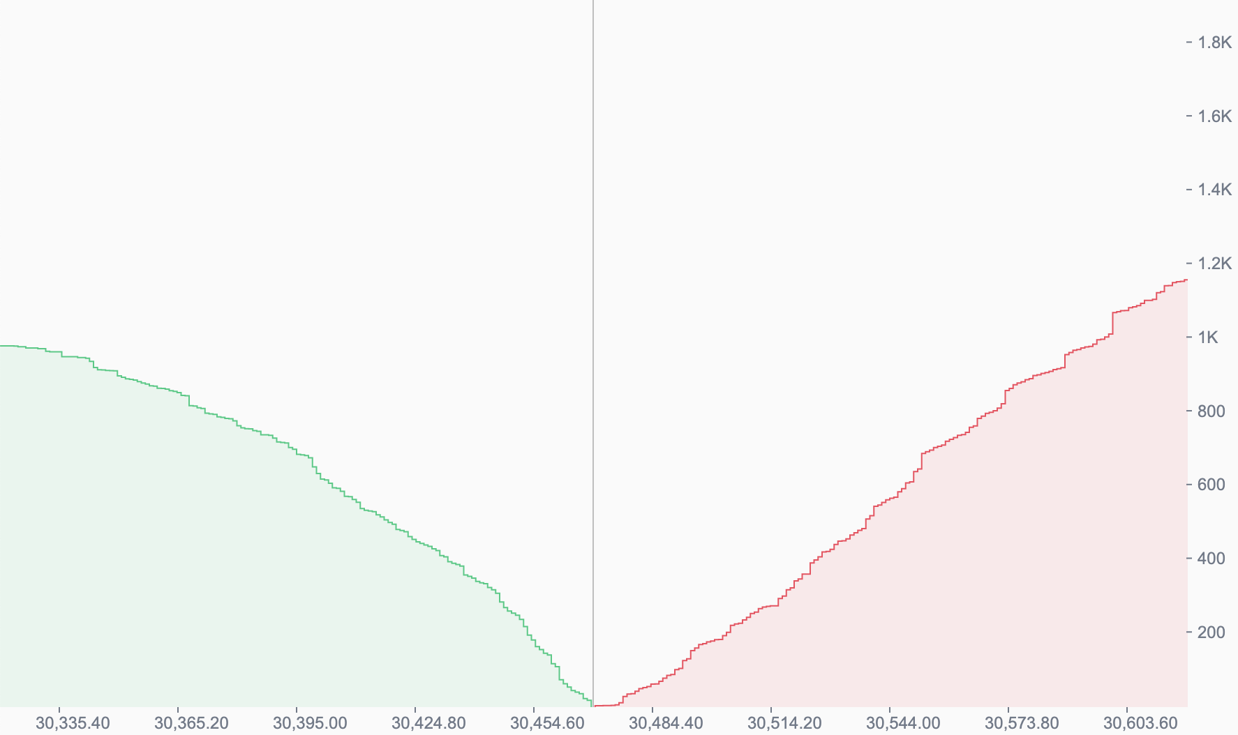
Figure 1: Binance BTC/USDT limit order book snapshot. Bid side (in green) represents the cumulative BTC quantity of buy limit orders, and ask side (in red) represents the cumulative BTC quantity of sell limit orders. The displayed BTC market price in USDT (vertical line) is the mid price, which is the average of the best bid price and the best ask price.

Cryptoassets are currently traded on two different types of exchanges: centralized exchanges (CEXs) and decentralized exchanges (DEXs). Centralized exchanges, such as Binance, Kraken, Coinbase (and previously, FTX) operate using limit order books. Figure 1 presents a snapshot of Binance BTC/USDT limit order book, with the bid side (in green) representing the cumulative BTC quantity of buy limit orders, and the ask side (in red) representing the cumulative BTC quantity of sell limit orders. In limit order markets, liquidity is usually provided by professional market makers, who strategically compete with each other by submitting limit orders.

[Insert Figure 1 approximately here]

In contrast, decentralized exchanges operate directly on a blockchain, with liquidity usually provided through an “automated market maker” (AMM). An AMM just follows a set of pre-programmed rules, so-called “smart contracts”, such that there is no explicit human intervention required when a trade (or a so-called “swap”) is submitted. Each asset pair, for example, ETH/USDC, comprises a separate liquidity pool. Liquidity providers (LPs), including retail investors, can deposit (“mint”) liquidity to the pool by adding both assets, or so-called tokens, in a respective ratio. They can also withdraw (“burn”) liquidity from the pool at a later point in time. Liquidity demanders (traders) can then swap one token for another in the pool at the current market price. Thus, in contrast to limit order markets, proper matching of buy and sell orders is not required in an AMM. All trades are executed against the AMM, with the market price determined by mathematical formulas in smart contracts. Liquidity demanders pay a pre-specified exchange fee, e.g. 0.3%, for each trade as a compensation to liquidity providers. Both liquidity demanders and liquidity providers have to pay additional transaction fees, so-called “gas fees”, as a compensation to miners who actually record their transactions (i.e. “swaps”, “mints”, “burns”) on the blockchain. Importantly, DEXs users keep custody of their assets, because they execute trades from their own wallets and settlement is immediate.

Uniswap is the leading decentralized exchange, with its first version, Uniswap v1, launched on Ethereum on November 2, 2018. The main drawback of Uniswap v1 is that it only supports trading against ETH, i.e. selling DAI for USDC requires two transactions: first, selling DAI for ETH and, second, ETH for USDC. To overcome this problem, Uniswap v2 was released in May 2020. Importantly, Uniswap v2 does not allow for competition of liquidity providers. The only decision liquidity providers make is whether to deposit liquidity in the pool or not. The trading fee equals 0.3% for all pools on Uniswap v2. Fees earned from trades are distributed pro-rata to liquidity providers, i.e. in proportion to the amount of liquidity they provide in the pool. Therefore, all gains (and losses) are mutualized by liquidity providers.

The latest version, Uniswap v3, was released in May 2021, implementing two main changes to Uniswap v2. First, it allows some degree of competition on price between liquidity providers by introducing the so-called “concentrated liquidity”. Specifically, when depositing their tokens, LPs can now indicate the price range, i.e. the minimum and the maximum prices in a given pool at which their liquidity position is active. However, there is no competition on speed available, as all gains for LPs within the same price range are still mutualized. Second, Uniswap v3 allows for four various fee tiers: 0.01%, 0.05%, 0.3% and 1%. Therefore, the same pair of assets can potentially be traded in four different pools. We discuss mechanics of trading on Uniswap v3 in more detail in Appendix B.

As of August 2022, $914B were traded on CEXs, out of which $443B were traded on Binance. Panel A of Figure 2 shows monthly traded volume on CEXs (in $) from May 2017 to April 2023. Among all CEXs, Binance is dominating, with an average market share of 50%.

[Insert Figure 2 approximately here]

Total traded volume on DEXs is 12 times lower than on CEXs as of August 2022, around $75B. However, it fluctuates considerably, with high values of $182B in November 2021 and $112B in March 2023, and low values of $39B in December 2022. Panel B of Figure 2 shows monthly trading volume on DEXs (in $) from January 2020 to April 2023. Uniswap v3 is the leading DEX with a market share of 58% in August 2022, followed by PancakeSwap with 11% and Curve with 8%. As Uniswap v3 is leading in terms of its market share among DEXs, we focus our analysis on this DEX in our paper.

2.2 Blockchain scaling solutions: Arbitrum and Polygon

Whereas Ethereum is currently the most secure blockchain with a number of validators exceeding 500,000 as of January 2023, its main disadvantage is low scalability. Specifically, a block is added to Ethereum every 12 seconds after the so-called Merge, i.e. when Ethereum moved to proof-of-stake consensus on September 15, 2022. Previously, with the proof-of-work consensus, block time was probabilistic and averaged between 13-15 seconds. Importantly, low scalability of Ethereum results in high gas fees, with an estimated average of gas fees for a trade on Uniswap v3 amounting to $14 in 2022.

To address the scalability issue, there exist overlays of Ethereum that offer higher speed and, more importantly, lower gas fees. Arbitrum and Polygon are two of the most adopted Ethereum scaling solutions. Currently, Uniswap v3 has also launched on the following Ethereum scaling solutions: Optimism, Celo, BNB Smart Chain, Base and Avalanche. We conduct our study on Arbitrum and Polygon, because they have the highest total value locked (TVL) and trading volume, in comparison to other solutions.

2.2.1 Entry of Arbitrum

Uniswap v3 launched on Arbitrum on August 31, 2021. Arbitrum is a “rollup”, i.e. a Layer 2 (L2) scaling solution that involves “rolling up”, or accumulating, transactions on Arbitrum in “batches”, subsequently compressing them and posting them on the Layer 1, i.e. Ethereum. This periodic posting allows Arbitrum to inherit Ethereum’s security, subject to the posting delay. Arbitrum uses a particular type of rollup - so-called optimistic rollup - that processes off-chain transactions optimistically, assuming validity by default and relying on occasional on-chain verification.

The main benefit of rollups is that the Layer 1 blockchain, i.e. Ethereum, does not need to validate separate transactions, but only batches of transactions. Therefore, Arbitrum (and other rollups) can offer higher speed by processing and batching transactions off-Ethereum before settling them on the main network. Average block time on Arbitrum was around 1-2 seconds at the beginning of 2022, subsequently dropping to around 0.25 seconds in 2023..

Importantly, transaction batching also allows rollups to offer much lower gas fees than Ethereum. Indeed, the gas price of a transaction on Arbitrum can be split into two parts: a part linked to the rollup network itself, which can be considered stable (it starts at 0.1 Gwei, i.e. one-billionth of ETH, and can increase with congestion), and a part linked to the posting of batches on Ethereum, which varies depending on Ethereum’s gas price. Batch data is compressed to reduce the cost of posting on Ethereum as much as possible. Still, posting batches on Ethereum represents a significant cost for rollups, with Arbitrum offering gas fees between $0.2 and $2 for a trade on Uniswap v3.

2.2.2 Entry of Polygon

Uniswap v3 launched on Polygon PoS (proof-of-stake) four months later than on Arbitrum, in December 2021. Polygon PoS is different to rollups, because it is a sidechain that requires its own security and decentralization efforts. In contrast to Arbitrum and other rollups, it does not automatically derive its security from the main blockchain, i.e. Ethereum. Specifically, Polygon is secured by a proof-of-stake consensus mechanism. However, Polygon still depends on Ethereum, because all the staking management is defined on Ethereum The overall number of validators on Polygon is lower, compared to Ethereum, but it still has a decent level of decentralization with over 100 unique validators. Whereas security of Polygon is not as robust as Ethereum’s, fewer validators can achieve consensus more quickly, hence leading to a shorter time between blocks and higher overall throughput. Average block time on Polygon is around 2-3 seconds, compared to Ethereum’s 12 seconds. Thus, Polygon can handle around 700 transactions per second (TPS), up to 70 times Ethereum’s TPS. Further, Polygon’s gas fees are the lowest, around $0.01 per transaction.

Polygon’s and Arbitrum’s liquidity pools are separate to those on Ethereum, i.e. liquidity is fragmented across pools. Thus, the same liquidity pool, ETH/USDC 0.05% for example, can exist on multiple chains, Ethereum, Polygon, Arbitrum and other scaling solutions. In our following analysis, we use the launch of Uniswap v3 on Arbitrum and Polygon as an instrument to identify the effect of lower gas fees on liquidity and its distribution around the market price.

3 Data and summary statistics

We analyze the two most liquid pairs on Uniswap v3, ETH/USDC 0.05% and ETH/USDC 0.3%, that are traded across all three chains: Ethereum, Arbitrum and Polygon. Hence, our benchmark sample consists of six distinct pools. For comparability across chains, we always use ETH as the base token and USDC as the quote token, i.e all data are presented for the ETH/USDC pair. ETH/USDC 0.05% is a low-fee pool that charges 5bp for each trade, or swap (in addition to the gas fee on the respective chain). ETH/USDC 0.3% is a high-fee pool that charges 30bp for each swap (in addition to the gas fee). Our sample period starts after the launch of Uniswap v3 on Polygon, on January 1, 2022, and ends on June 30, 2023. We download historical logs of Ethereum, Arbitrum and Polygon transactions (swaps, mints and burns on Uniswap v3), using The Graph queries.

Panel A of Table 1 compares volume and liquidity for both low- and high-fee pools across Ethereum, Arbitrum and Polygon. Specifically, we report the average trading volume over the previous 24 hours and the average liquidity size, measured as total value locked (TVL), both in $M.

[Insert Table 1 approximately here]

Unsurprisingly, both volume and TVL on Ethereum significantly exceed those on scaling solutions. For example, the average 24-hour volume for Ethereum’s most liquid pool, ETH/USDC 0.05%, is $513.73M, around 10 times higher than Arbitrum’s $51.93M and 18 times higher than Polygon’s $29.03M. Ethereum’s average TVL of $201.19M is around 11 times higher than Arbitrum’s $18.04M and around 20 times higher than Polygon’s TVL of $10.26M. Notably, the turnover, measured as the ratio of volume to TVL, is approximately the same across all three chains (as reported in the last column of Table 1). We observe much lower trading volume and TVL for the high-fee pool, ETH/USDC 0.3%, especially on Arbitrum and Polygon. These findings are consistent with theoretical predictions of [16] that lower gas fees lead to lower fragmentation of liquidity across high- and low-fee pools. As gas fees on Arbitrum and Polygon are relatively cheap, it is optimal for LPs to actively manage their positions in the low-fee pool. Thus, most of liquidity provision takes place on the low-fee pool on Arbitrum and Polygon, and not on the high-fee pool.

We further provide summary statistics of trade sizes and trade frequencies in Panels B and C of Table 1. Panel B shows that the average trade size on Ethereum is significantly larger for both pools. For example, the average trade size for ETH/USDC 0.05% on Ethereum is around $72K. In contrast, Arbitrum’s and Polygon’s average trade size for this pool are much lower, around $4K and $2.5K, respectively. We observe even lower trade sizes on Arbitrum and Polygon for ETH/USDC 0.3%, most likely because of their overall lower TVL on these scaling solutions. In contrast, we observe that the high-fee pool has a larger average trade size of $116K on Ethereum, compared to the low-fee pool. This finding is consistent with the theory of [10] that pools with higher fees attract more liquidity providers, increasing their TVL and attracting larger trades.

Panel C of Table 1 reports the average daily number of trades as well as the average daily number of purchases and sales across the three chains. Strikingly, both Arbitrum and Polygon have almost twice as many trades, around 12.5K per day, compared to Ethereum’s 7K for ETH/USDC 0.05%. For ETH/USDC 0.3%, the number of trades is approximately the same across all chains. For all pools, the order flow is balanced, i.e. the average daily number of buys is approximately equal to the average daily number of sells. We also report the average time between the trades (in seconds) in the last column. Overall, we conclude that the higher volume on Ethereum is mostly driven by larger trades being executed on this chain. In contrast, Arbitrum and Polygon are rather used by smaller traders who trade more frequently.

As discussed in Section 2.2, Ethereum’s larger liquidity can be explained by its higher security. Liquidity providers would like to minimize the risk of losing their funds, especially so for large liquidity deposits. Therefore, Ethereum is mostly used for large liquidity deposits, resulting in higher TVL. Large traders are also attracted to Ethereum, both due to its higher security and larger liquidity, which helps them reduce the slippage of their trades. Since gas fees are fixed, they are not of primary concern for large traders. In contrast, blockchain scaling solutions are rather attractive for smaller traders, who are primarily concerned about gas fees, and less so about security. Thus, we observe a separating equilibrium, in which large traders and LPs choose Ethereum due to its higher security, whereas small traders and LPs choose Arbitrum and Polygon due to their lower gas fees.

Table 2 reports summary statistics of control variables, which we use later in our regressions: trading volume over the previous 24 hours, $Volume$, (in $M); the 1-minute return of ETH/USD, $Return$ (in bp); and the realized volatility of ETH/USD, $Volatility$, computed as the square root of the sum of squared 1-minute returns over the previous 24 hours (in %). Both $Volatility$ and $Return$ are based on a single time series for ETH/USD from Binance. 1-minute returns are strongly balanced, with positive and negative returns being of approximately the same magnitude, with both the average and the median $Return$ close to zero. The average daily realized volatility of 3.53% of ETH/USD corresponds to an annualized volatility of 67.44%. Appendix E provides a detailed description of all variable definitions.

4 Repositioning and liquidity concentration

In this section, we test the effect of lower gas fees, provided by blockchain scaling solutions, on liquidity concentration around the current pool price. We start with formulating our hypotheses in Section 4.1. We then test the causal relation between repositioning intensity and liquidity concentration, using instrumental variable regressions, in Section 4.2. Section 4.3 examines the causal relation between repositioning precision and liquidity concentration.

4.1 Hypotheses development

Higher speed of transaction processing and lower gas fees on blockchain scaling solutions allow liquidity providers to update their positions more frequently. Should a permanent price change occur, LPs can withdraw and re-deposit their positions, re-setting the price range around the new market price more quickly and at a cheaper cost. Thus, higher speed and lower gas fees help LPs better protect their positions from adverse selection by arbitrageurs. Being able to better protect themselves, LPs can earn higher fees (for the same deposited amount) by concentrating their positions around the market price.

In contrast, when updating is costly, we expect LPs to post their liquidity on wider price ranges. In absence of updating, posting on a wider range provides better protection from adverse selection relative to a narrow price range. Therefore, we expect less frequent updating when gas fees are higher, with LPs updating their positions only if the market price significantly deviates from the position range. Wider liquidity positions should then result in less concentrated aggregate liquidity around the market price.

[Insert Figure 3 approximately here]

Figure 3 further illustrates our predictions with a stylized numerical example. In Panel A, we assume that ETH price (in USDC) experiences a permanent increase from 1,000 to 2,000. Without updating, an LP’s position is adversely selected by an arbitrageur, who submits a buy trade. The arbitrageur’s trade moves the market price to the new level, depleting all ETH reserves in the LP’s position and leaving him only with USDC. The LP experiences an adverse selection loss of $500K, compared to the scenario, in which he would just buy and hold his initial portfolio of ETH and USDC, without providing liquidity on a DEX.

Panel B shows that the LP could partially protect himself from adverse selection by redistributing the same amount of capital on a wider price range. Thus, his position would be less concentrated around the market price. Posting on a wider price range would reduce LP’s losses to $300K, because average execution price for his ETH reserves would be higher, compared to Panel A. In contrast, Panel C assumes that the LP continuously monitors the market and is able to update his position even before the arbitrageur’s trade arrives. In this scenario, the LP is able to fully avoid adverse selection loss and makes a profit of $500K. It is optimal for him to set a narrower price range, i.e. make his position more concentrated, in order to earn higher rewards.

Being able to immediately update is the first-best solution for any LP. However, updating is costly and requires continuous monitoring. Therefore, we expect LPs to reposition more frequently when updating is relatively cheaper, i.e. on blockchain scaling solutions. In the following, we refer to the position updating frequency of LPs as repositioning intensity. We formalize our first hypothesis as follows:

Hypothesis 1. Compared to Ethereum, higher repositioning intensity on blockchain scaling solutions leads to higher aggregate liquidity concentration around the current market price.

Whereas we use repositioning intensity as our benchmark measure, it could be that liquidity providers do not necessarily update their positions close to the new market price. Specifically, repositioning intensity does not take into account whether liquidity positions are centered around the market price or not. Further, a position might be centered around the market price, but it could also have a wide price range, which should not necessarily result in higher liquidity concentration. To address these issues, we also focus our analysis on repositioning precision, which we define as the distribution of individual liquidity positions around the market price.

Specifically, we expect repositioning precision to be higher on blockchain scaling solutions. With lower gas fees and better protection from adverse selection, we expect LPs to make their positions more concentrated around the market price, i.e. we expect them to re-post on a narrow price range, with the mid-price of the range close to the current market price. More concentrated individual positions allow LPs to maximize their rewards from liquidity provision. Importantly, more concentrated individual positions should result in higher aggregate liquidity concentration around the current market price. Based on these predictions, we formalize our second hypothesis as follows:

Hypothesis 2. Compared to Ethereum, higher repositioning precision on blockchain scaling solutions leads to higher aggregate liquidity concentration around the current market price.

Higher liquidity concentration around the market price is important, because it affects slippage. In this paper, we define slippage of a trade as the difference between the average execution price and the observed pre-execution market price. For a given TVL, higher liquidity concentration around the market price should reduce the slippage of any trade. In contrast, less concentrated aggregate liquidity should increase slippage for a given TVL.

Importantly, Arbitrum’s and Polygon’s TVL is significantly lower than Ethereum’s (see Panel A of Table 1). Ethereum’s large TVL, which corresponds to overall market depth, is still of first-order importance for slippage of large trades, relative to liquidity concentration. Hence, we expect large trades to have overall lower slippage on Ethereum due to its higher TVL. Based on these differences in observed TVL, slippage is only comparable for smaller trades (up to $5K) between Ethereum and blockchain scaling solutions. Therefore, we formalize our third hypothesis as follows:

Hypothesis 3. Higher liquidity concentration on blockchain scaling solutions should result in lower slippage for small trades (up to $5K), compared to Ethereum. For large trades (above $5K), slippage should be lower on Ethereum due to its higher TVL.

4.2 Repositioning intensity and liquidity concentration

Liquidity concentration. We start by comparing aggregate liquidity concentration around the market price across Ethereum and blockchain scaling solutions. Specifically, we define liquidity concentration within x% of the market price, as the market depth within x% of $p_{mkt}$, divided by $TVL$. Market depth within x% of $p_{mkt}$ is computed as the dollar value of the liquidity between $\frac{p_{mkt}}{1+x\%}$ and $p_{mkt}\cdot(1+x\%)$. Table 3 reports average levels of liquidity concentration across Ethereum, Arbitrum and Polygon, separately for low-fee and high-fee pools.

[Insert Table 3 approximately here]

Column (1) reports average levels of liquidity concentration within 1% of the market price. Columns (2) and (3) report corresponding statistics for liquidity concentration within 2% and 10% of the market price, respectively. Liquidity concentration mechanically increases with the percentage band, i.e. market depth as percentage of TVL within 10% of the market price is by construction higher than within 1% of the market price. More surprisingly, only around 24%-42% of all liquidity is concentrated within 10% for all pools. Hence, around two thirds of TVL are further away than 10% from the market price across all pools. Consistent with our expectations, we find strong evidence for higher liquidity concentration on blockchain scaling solutions across all percentage bands, compared to Ethereum. We observe the differences between average liquidity concentration on Arbitrum and Ethereum, $\Delta Arb-Eth$, of 0.93%-5.36%. The corresponding numbers for differences between Polygon and Ethereum, $\Delta Pol-Eth$, are 1.18%-14.54%. T-statistics of the two-tailed t-test with the null-hypothesis of difference equaling zero all exceed 100, i.e. all differences are statistically significant at the 1% level.

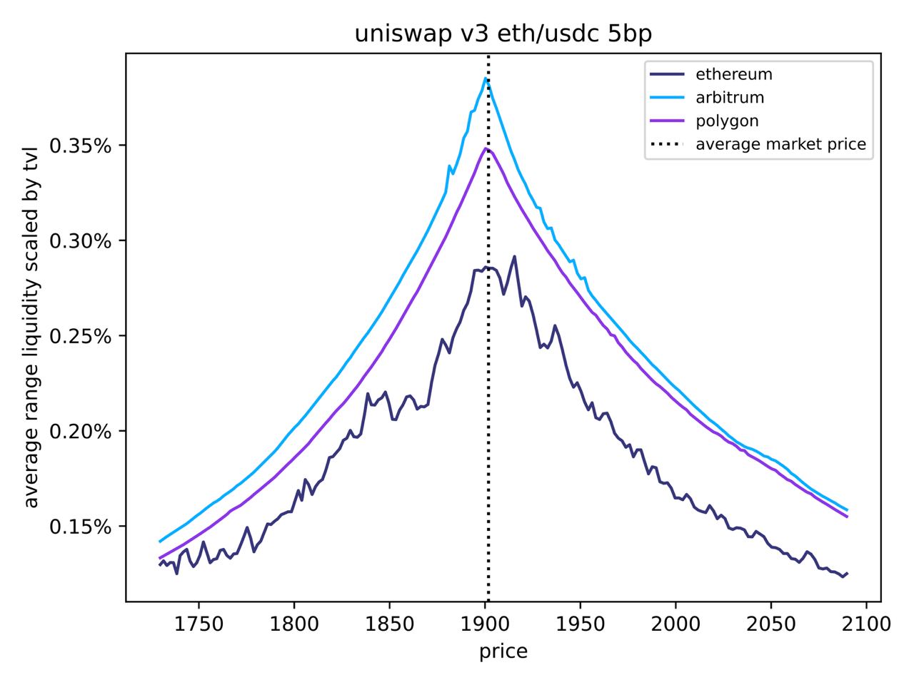
Figure 4: Average range liquidity, scaled by TVL: ETH/USDC 0.05%. This figure shows average liquidity within each price range, scaled by TVL, for ETH/USDC 0.05% pool, separately for Ethereum, Arbitrum and Polygon. Averages for each price range are constructed from hourly liquidity snapshots over our sample period January 1, 2022 - June 30, 2023. The dotted vertical line shows the average market price over our sample period.

Figure 4 further illustrates the distribution of aggregate liquidity around the market price for ETH/USDC 0.05% pool, separately for Ethereum, Arbitrum and Polygon. Specifically, we use hourly snapshots to calculate average liquidity within each price range, scaled by TVL (in %), over our sample period January 1, 2022 - June 30, 2023. Consistent with our findings in Table 3, we observe higher liquidity concentration around the market price for Arbitrum and Polygon, relative to Ethereum, i.e. liquidity distribution is more ”peaked” for blockchain scaling solutions.

[Insert Figure 4 approximately here]

Liquidity provision and repositioning intensity. We further examine differences in liquidity provision and repositioning intensity across Ethereum and blockchain scaling solutions in Table 4. For all our analyses of liquidity provision, we filter out liquidity mints and burns, for which the mid price of their range, computed as $\sqrt{p_{lower}\cdot p_{upper}}$, lies further than 20% away from the market price. We treat these mints and burns as outliers and exclude them from our analysis. We further exclude so-called “just-in-time” (JIT) liquidity positions, which are used to provide “flash” liquidity within the same block to large trades on Ethereum towards the end of our sample. JIT positions represent around 27% of our sample on Ethereum and less than 2.5% on Arbitrum and Polygon. We exclude them, since this “flash” liquidity does not affect TVL and thus, liquidity concentration, which is our main variable of interest. Further, JIT liquidity provision only benefits a few large traders on Ethereum, and is generally not used to provide liquidity for small trades.

[Insert Table 4 approximately here]

We report the average daily number of mints for each chain in column (1) and the average daily number of burns in column (4). Compared to Ethereum, we observe significantly more frequent minting and burning of liquidity on Arbitrum and Polygon for ETH/USDC 0.05% pool. A mint on Arbitrum (Polygon) takes place on average every 4.57 (2.63) minutes and a burn every 6.05 (3.88) minutes, as compared to Ethereum’s 17.73 and 23.40 minutes, respectively (see columns 2 and 5). However, the average daily minted value on Arbitrum (Polygon) of around $11.75M ($2.95M) is significantly lower than $41.19M minted daily on Ethereum (column 3). Average daily burned values on Arbitrum and Polygon are of approximately the same magnitude as daily minted values, and also significantly lower than Ethereum’s $39.9M (column 6).

For ETH/USDC 0.3%, the daily number of mints is approximately the same across Ethereum and blockchain scaling solutions, with a mint occurring every 20 minutes on each of the chains. The daily minted value is much lower on Arbitrum and Polygon, which is consistent with our prior findings of overall lower TVL for high-fee pools on blockchain scaling solutions. Consequently, the daily burned value is also lower for high-fee pools on Arbitrum and Polygon. These findings further support predictions of [16] that all liquidity mostly consolidates in the low-fee pool in presence of low gas fees.

More frequent minting and burning liquidity on blockchain scaling solutions, especially for the low-fee pool, suggests more intense liquidity repositioning. We next measure repositioning intensity, $Intensity$, more explicitly. Specifically, we define repositioning as a burn, followed by a mint, in the same pool by the same liquidity provider within next five minutes. In the following, we refer to mints, associated with repositioning, as ”repositioning mints”. We then compute repositioning intensity as the dollar value of repositioning mints over a 5-minute interval, divided by the total dollar value minted over the same interval:

$$Intensity=\frac{RepositioningMinted_{\$}}{TotalMinted_{\$}},$$ (1)

$Intensity$ can take values between 0 and 1, with higher values associated with more intense repositioning. We use five minutes as our benchmark time interval for computing intensity, because it represents the average time between all mints and burns in our sample. However, we also check that all our results are robust if we use the median time of one minute between all mints and burns in our sample instead.

Column (7) of Table 4 presents the average 5-minute repositioning intensity (in %) across Ethereum, Arbitrum and Polygon. For ETH/USDC 0.05%, the repositioning intensity on Arbitrum (Polygon) is 40.64% (35.90%), which is more than double as high, compared to Ethereum’s 15.89%. For ETH/USDC 0.3% we observe overall lower levels of intensity across all three chains, as compared to the low-fee ETH/USDC 0.05% pool. Indeed, high-fee pools are mostly used by more passive liquidity providers (LPs), consistent with prior findings of [16]. Importantly, $Intensity$ on both Arbitrum and Polygon of 17.10%-24.78% is still two to three times higher for the high-fee pool, relative to Ethereum’s 7.29%. Overall, as expected, we observe significantly more repositioning taking place on blockchain scaling solutions, driven by higher speed of transaction processing and lower gas fees.

Instrumental variable (IV) regressions. So far, we find that both liquidity concentration and repositioning intensity is significantly higher on blockchain scaling solutions, relative to Ethereum. In this section, we would like to explicitly test our Hypothesis 1, showing the causal relation between repositioning intensity and liquidity concentration on DEXs. The straightforward approach to test this association is by regressing liquidity concentration on repositioning intensity and other variables, controlling for market conditions. However, the choice of an LP to update their position, i.e. burn and subsequently mint at a new price range, is potentially endogenous, and can in itself depend on the current liquidity concentration in the pool. Hence, the slope coefficient on repositioning intensity from standard OLS estimation would represent a biased estimate of its causal effect on liquidity concentration.

To identify the causal effect of repositioning intensity, we use the launch of Uniswap v3 on Arbitrum and Polygon as our instrument for an exogenous increase in updating frequency of LPs. For any instrument to be valid, it has to satisfy two criteria. First, the instrument must be correlated with the endogenous explanatory variable, i.e. it should induce change in the explanatory variable. Second, it must satisfy the exclusion restriction, i.e. it should not be correlated with the error term in the explanatory equation. The first condition holds, because we indeed observe more frequent repositioning by LPs on blockchain scaling solutions as a result of much lower gas fees (see Table 4). For exclusion restriction to hold, Uniswap’s launch on blockchain scaling solutions should not affect liquidity concentration other than through its effect on repositioning intensity. We argue that such correlation with the error term is rather unlikely, because it would mean that Uniswap v3 chose its entry date on Arbitrum (Polygon) strategically and was able to accurately predict a market-wide increase in liquidity concentration. Our setup is similar to [13], who use the

introduction of NYSE Autoquote as an instrument for an exogenous increase in algorithmic trading, and investigate its causal effect on liquidity.

To test the causal relation between repositioning intensity and liquidity concentration, we next run instrumental variable regressions. We first estimate the following first-stage regression, separately for each pool:

$$Intensity_{t} = \alpha+\beta_{1}Arbitrum/Polygon{}_{t}+$$

$$+ \beta_{2}Volume{}_{t}+\beta_{3}Volatility{}_{t}+\beta_{4}|Return|{}_{t}$$

$$+ HourFE+DayFE+\varepsilon_{i,t},$$

where $Arbitrum$ ($Polygon$) takes value of 1 for Arbitrum (Polygon) pool, and equals zero for the corresponding Ethereum pool. $Intensity$ and $|Return|$ are measured over 5-minute intervals. $Volume$ is the volume over previous 24 hours and $Volatility$ is the realized volatility over previous 24 hours, both measured at the end of each 5-minute interval. All regressions include hour- and day-fixed effects and allow standard errors to cluster at the day level.

[Insert Table 5 approximately here]

Panel A of Table 5 reports the results for ETH/USDC 0.05%. The coefficient of 0.24 on $Arbitrum$ in Model (1) implies that repositioning intensity is 24% higher on Arbitrum for this pool, relative to Ethereum. This coefficient is consistent with our previous statistics on $\Delta Arb-Eth$ from Table 4. We find that repositioning intensity on Polygon is also significantly higher by 20%, relative to Ethereum (Model 3). We next include both Arbitrum and Polygon pools in one regression. In Model (5), we define $BlockScaling$ as an indicator variable that takes value of 1 for Arbitrum and Polygon pools, and zero for the Ethereum pool, used as a benchmark. On average, we observe 21% higher repositioning intensity on blockchain scaling solutions, relative to Ethereum.

Models (2), (4) and (6) report corresponding results for the second-stage regression:

$$Conc_{t} = \alpha+\beta_{1}Intensity{}_{t}+$$

$$+ \beta_{2}Volume{}_{t}+\beta_{3}Volatility{}_{t}+\beta_{4}|Return|{}_{t}$$

$$+ HourFE+DayFE+\varepsilon_{i,t},$$

Liquidity concentration, $Conc$, is measured within 2% of the current market price at the end of each 5-minute interval. The set of instruments consists of all explanatory variables, except that we use $Arbitrum$ in place of $Intensity$ in Model (2). In Models (4) and (6), we use $Polygon$ and $BlockScaling$ in place of $Intensity$, respectively. Overall, Models (2), (4) and (6) show that an increase in repositioning intensity significantly increases liquidity concentration within 2% of the market price. The IV estimates of 0.09-0.11 on $Intensity$ variable mean that a 1% increase in $Intensity$ increases liquidity concentration by around 10% for ETH/USDC 0.05% pool. The average standard deviation for $Intensity$ is 0.4384 for this pool, such that a one-standard deviation change in $Intensity$ is associated with a $0.4384\cdot 0.10=0.0438$ or 4.38% change in liquidity concentration. This value is economically significant, because it represents a 43% increase from the mean liquidity concentration (within 2% of the market price) of 10.16% on Ethereum.

We also observe a significant effect of repositioning intensity on liquidity concentration for the high-fee pool in Panel B, with IV estimates on $Intensity$ of 0.08 for Arbitrum and 0.22 for Polygon. Table 4 shows that an increase in the repositioning intensity is higher on Polygon for this pool, hence we observe a stronger effect, relative to Arbitrum.

To analyze which subset of LPs are actively engaging in repositioning, we next split LPs by their aggregate minted and burned dollar value in each pool. In other words, for each LP, we sum up their total minted and burned liquidity (in $) over our entire sample period, separately for each chain and each pool. We then define large LPs as those in the top quartile of our sample distribution, i.e. those with the highest dollar value minted and burned. We replicate our previous analysis from Table 5 for a subset of large LPs. Unsurprisingly, they are practically identical to our benchmark findings in Table 5 (see Table IA1 in the Internet Appendix). Overall, these findings suggest that repositioning is indeed largely done by the largest (professional) liquidity providers on each chain.

Robustness checks. Table 6 presents robustness checks of our main findings. Panel A presents results for the low-fee pool, and Panel B for the high-fee pool. Models (1) and (2) report results of the second-stage IV regressions with $BlockScaling$ as an instrument for the low-fee pool (similar to our benchmark Model 6 in Table 5), using liquidity concentration within 1% and within 10% of the current market price as the dependent variable, respectively. We observe that the effect of repositioning intensity on liquidity concentration increases with the percentage band, i.e. it affects liquidity concentration within 10% (2%) to a larger extent than within 2% (1%). This effect is likely due to more repositioning taking place within 10% (2%) of the market price, as opposed to repositioning within 2% (1%).

[Insert Table 6 approximately here]

Model (3) replicates our analysis from benchmark Model (6) in Table 5, using an alternative measure for repositioning intensity, $IntensFreq$, defined as the ratio of the number of repositioning mints to the total number of mints within a 5-minute interval. The IV estimate on $IntensFreq$ of 0.24 for the low-fee pool is even higher, compared to the benchmark estimate of 0.11 from Panel A of Table 5. Model (4) uses another alternative measure of $Intensity$, based on the 1-minute repositioning mints, which is the median time between all mints and burns in our sample. In this analysis, we classify repositioning mints as those that are preceded by burns of the same LP within the previous minute. The IV estimate of 0.16 is of comparable economic magnitude to our benchmark estimate. In Model (5), we use aggregation, based on 10-minute intervals instead of 5-minute intervals. The results are practically identical to our benchmark estimate. We also observe similar patterns for all robustness tests for the high-fee pool in Panel B.

To sum up, we find strong empirical evidence for our Hypothesis 1. Our instrumental variable regressions show that higher repositioning intensity on blockchain scaling solutions indeed leads to higher aggregate liquidity concentration around the current market price, both for the low-fee and the high-fee pools.

4.3 Repositioning precision and liquidity concentration

Repositioning precision. We next test our Hypothesis 2 about the causal link of repositioning precision and aggregate liquidity concentration around the current market price. We use three measures for repositioning precision: position gap, position length and position precision. Our first measure is position gap, $Gap$, computed as $\left|\frac{p_{mid}}{p_{mkt}}-1\right|$, where $p_{mid}$ is the mid price of the position. For each position, posted on the range $[p_{lower},p_{upper}]$, we compute $p_{mid}$ as $\sqrt{p_{lower}\cdot p_{upper}}$. The lower the position gap, the closer the mid price of minted positions to the market price. Therefore, $Gap$ is inversely related to repositioning precision. We report the average position gap (in %) across all repositioning mints in Column (1) of Table 7.

[Insert Table 7 approximately here]

For ETH/USDC 0.05%, we observe the average position gap of 1.86% on Ethereum, i.e. liquidity providers re-position their mints on average 1.86% away from the market price. Consistent with our prior expectations, we find that the average position gap on blockchain scaling solutions is significantly lower by 0.8%-1%, which represents an improvement in repositioning precision of around 50%. For the high-fee pool, the average position gap on Ethereum is higher, 3.41%, because liquidity providers do not reposition as often for this pool, compared to the low-fee pool. However, we also observe significant precision improvement on blockchain scaling solutions for this pool by around one third (i.e. by 1%-1.3%).

Our second measure of repositioning precision is position length, $Length$, computed as $\frac{\lvert p_{upper}-p_{lower}\rvert}{p_{mid}}$. The shorter the position length, the narrower the position is. Similar to $Gap$, it is inversely related to repositioning precision. We report the average position length (in %) across all repositioning mints in Column (2) of Table 7. For the low-fee pool, we observe that positions are significantly narrower by 7.38% on Arbitrum and 5.16% on Polygon, relative to the average value of around 18% on Ethereum. For the high-fee pool, positions are overall substantially wider on Ethereum, in the range of 30%. This result is consistent with more passive liquidity providers (with lower repositioning intensity) posting wider ranges on high-fee pools to protect themselves from adverse selection. Importantly, we observe substantially narrower positions in this pool on blockchain scaling solutions by around 14%. This substantial reduction in position length for the high-fee pool is due to lower gas fees on Arbitrum and Polygon. With low gas fees, it is cheaper, even for relatively more passive (i.e. retail) liquidity providers, to update their positions, protecting themselves from adverse selection.

The previous two measures look separately at the mid price of the position range and on its length. Our third measure, position precision, $Precision$, combines the previous two to address a potential criticism that positions with lower gaps could potentially be wider, or, alternatively, narrower positions could be posted further away from the market price. We compute $Precision$ as $\frac{1}{Gap\cdot Length}$ and further scale it to lie in the range [0,1] as $1-1.0001^{\frac{-1}{Gap\cdot Length}}.$ $Precision$ has the lowest possible value of 0 and the highest possible value of 1, or 100%. As for other measures, we compute the average precision across all repositioning mints.

Column (3) of Table 7 shows that position precision is indeed significantly higher on blockchain scaling solutions, relative to Ethereum. For ETH/USDC 0.05%, $Precision$ is higher by 18%-20%, relative to the average value of 51% on Ethereum. As expected, position precision is generally lower for the high-fee pool with more passive liquidity providers, around 20% on Ethereum. Importantly, it almost doubles on blockchain scaling solutions, increasing by 17% on Arbitrum and by 22% on Polygon.

Overall, our univariate results confirm that liquidity providers re-position on Arbitrum and Polygon not only closer to the market price, but also at significantly narrower ranges. Thus, lower gas fees result in both higher repositioning intensity and higher repositioning precision around the market price.

Instrumental variable (IV) regressions. We next test the causal relation between repositioning precision and liquidity concentration. Similar to repositioning intensity, repositioning precision is endogenous. To address this issue, we use the launch of Uniswap v3 on blockchain sclaing solutions as our instrument for an exogenous increase in repositioning precision. Since LPs are able to reposition more frequently on Arbitrum and Polygon, they are better able to protect themselves from adverse selection. Hence, for the same amount of capital deposited, LPs can maximize their rewards from liquidity provision by improving the precision of their positions, i.e. minting positions that are more concentrated around the market price. Indeed, our findings from Table 7 show that repositioning precision is significantly higher on both Arbitrum and Polygon, relative to Ethereum.

We re-estimate our previous instrumental variables regressions, with $Blockscaling$ now used as an instrument for repositioning precision. Table 8 reports results for instrumental variable regressions, separately for three measures of repositioning precision.

[Insert Table 8 approximately here]

Models (1) and (2) show results with position gap as a measure of repositioning precision. Model (1) reports results of the first-stage IV regression, with $Gap$ as the dependent variable and $Blockscaling$ as the main explanatory variable. Consistent with previous findings in Table 7, we observe significantly lower position gaps on blockchain scaling solutions, relative to Ethereum. Model (2) shows results of the second-stage IV regressions, with liquidity concentration within 2% of the market price as the dependent variable. Consistent with Hypothesis 2, we find that higher position gaps significantly reduce liquidity concentration around the current market price. The average standard deviation for $Gap$ is 0.023 for ETH/USDC 0.05%. Therefore, the IV estimate of -4.15 means that a one-standard deviation increase in $Gap$ is associated with a $0.023\cdot-4.15=-0.0954$ or 9.54% decrease in liquidity concentration. As expected, we also observe a significant negative effect of $Length$ (Models 3 and 4) and a significant positive effect of $Precision$ (Models 5 and 6) on liquidity concentration for both pools.

Consistent with our Hypotheses 1 and 2, our results in this section show that both repositioning intensity and precision increase liquidity concentration around the market price. As both these variables are potentially endogenous, we use the launch of Uniswap v3 on Arbitrum and Polygon as our instruments to identify the causal effect of repositioning intensity and precision on liquidity concentration. An increase in liquidity concentration is important because it reduces slippage, for a given TVL. In the next section, we explicitly compare slippage for trades of different sizes on Ethereum and blockchain scaling solutions.

5 Slippage: Ethereum vs blockchain scaling solutions

In this paper, we define slippage of a trade as the difference between the average execution price, $p_{avg}=\frac{\Delta y}{\Delta x}$ and the pre-execution pool price, $p_{mkt}$:

$Slippage=\left|\frac{p_{avg}}{p_{mkt}}-1\right|$

In other words, slippage shows by how much the execution price is worse than the previously displayed market price. Slippage is greater for larger trades and, as in [14], is inversely related to market depth. Appendix C discusses mechanics of trade execution and derivations of average execution prices on Uniswap v3. Appendix D provides a numerical example of slippage computation on DEXs.

We compute slippage, $Slippage$, for hypothetical trades of sizes [$100, $500, $1K, $5K, $10K, $50K, $100K] at the end of each 5-minute interval over our sample period (January 1, 2022 - June 30, 2023). Panel A of Table 9 presents summary statistics for $Slippage$ (in bp), separately for each chain.

[Insert Table 9 approximately here]

Given Ethereum’s overall larger TVL, it is not surprising that its average slippage of 0.3 bp for the low-fee pool is significantly lower than Arbitrum’s 8.8 bp and Polygon’s 4.25 bp. The median slippage of 0.60-0.73 bp on blockchain sclaing solutions is also higher, compared to Ethereum’s 0.05 bp. As expected, average and median slippage values are higher for the high-fee pool across all chains, due to its lower TVL. However, these statistics represent the average across both small hypothetical trades of $100, $500, etc. and large hypothetical trades of up to $100K. As Arbitrum and Polygon are mostly used by smaller traders, the main focus of our analysis will be the comparison of slippage for small trades across Ethereum and scaling solutions.

Before conditioning on trade size, we first confirm our findings from Panel A in a multivariate setup. Specifically, we estimate following OLS regressions:

$$Slippage_{i,t} = \alpha+\beta_{1}BlockScaling{}_{i,t}+\beta_{2}Size{}_{i,t}+$$

$$+ \beta_{3}Buy{}_{i,t}+\beta_{4}Volume{}_{i,t}+\beta_{5}Volatility{}_{i,t}+\beta_{6}|Return|{}_{i,t}$$

$$+ HourFE+DayFE+\varepsilon_{i,t}.$$

The dependent variable, $Slippage$, shows the slippage for a trade of a given size for pool $i$ at the end of each 5-minute interval $t$ (from the end-of-minute snapshot of liquidity distribution). As before, $BlockScaling$, equals 1 for transactions on Arbitrum and Polygon, and zero for Ethereum. Therefore, trades on Ethereum serve as a benchmark sample. The vector of control variables includes trade size (in $K), $Size$; the direction of the trade, $Buy$, that equals 1 for purchases of token X and 0 for its sales; trading volume over previous 24 hours (in $M), $Volume$; realized volatility of ETH/USD over previous 24 hours, $Volatility$; and absolute return of ETH/USD over the previous minute, $|Return|$. All regressions include hour- and day-fixed effects and allow standard errors to cluster at the day level.

Panel B of Table 9 reports results for ETH/USDC 0.05% pool. The coefficient on $BlockScaling$ in Model (1) shows that slippage on blockchain scaling solutions is on average 1.41 bp higher, relative to the average slippage on Ethereum, after including control variables. Unsurprisingly, slippage is increasing in the size of the trade. It does not differ significantly between buys of token X and its sells. Further, slippage is decreasing in the trading volume, implying that LPs deposit more liquidity if they observe higher volume over previous 24 hours. This finding is consistent with our prior expectations, because LPs can earn higher fees in periods of higher volume. Finally, slippage is increasing in both the absolute return of ETH/USD over the previous five minutes and the realized volatility over previous 24 hours. These findings are also in line with our expectations, suggesting that LPs are more likely to withdraw liquidity from the pool during times of higher uncertainty. We observe similar findings for the high-fee pool in Panel C, with slippage on average higher by 21.61 bp on blockchain scaling solutions,

We next test our Hypothesis 3, which predicts that higher liquidity concentration on blockchain scaling solutions should result in lower slippage for small trades. Hence, we condition our analysis on trade size, using the $1K and the $5K cutoffs to split trades into small and large categories. We use these cutoffs, because the 75th percentile of trades on both Arbitrum and Polygon never exceeds $5K, with average trade sizes of $2K-$4K (see Panel B of Table 1).

In Model (2), we add a dummy variable $Large$ that equals 1 for large trades that exceed the $1K cutoff, and zero otherwise. We also add its interaction term with $BlockScaling$, $BlockSc\cdot Large$, that captures the relative difference in slippage of large trades on blockchain scaling solutions, relative to Ethereum. The coefficient on $BlockScaling$ now captures the relative difference in slippage of small trades between Ethereum and blockchain scaling solutions, and is of main interest in our analysis. As $Large$ is mechanically related to $Size$, we omit $Size$ from the vector of our control variables in Model (2).

We observe a positive and significant coefficient on $Large$ in Model (2), suggesting that large trades on Ethereum (i.e. those in excess of $1K) have on average 0.51 bp higher slippage in the low-fee pool, compared to small trades. Importantly, we observe coefficients of different signs on $BlockScaling$ and $BlockSc\cdot Large$. The negative coefficient on $BlockScaling$ shows that slippage of small trades (less than $1K) on scaling solutions is by 4.6 bp lower, compared to small trades on Ethereum. The positive coefficient on the interaction term, $BlockSc\cdot Large$, shows that large trades on scaling solutions have a significantly higher slippage of 10.53 bp, relative to large trades on Ethereum. Hence, the overall positive coefficient on $BlockScaling$ in Model (1) is driven by significantly higher slippage for larger trades. Once we condition on trade size, we observe significantly lower slippage for small trades on Arbitrum and Polygon.

Model (3) reports similar results, using $5K cutoff to split trades into small and large categories. Models (4) and (5) report results separately for Arbitrum and Polygon, using $1K cutoff. Overall, we observe economically stronger effect for Arbitrum, most likely because Arbitrum pools are more liquid and have higher TVL, compared to Polygon (see Table 1). All results also hold for the high-fee pool (Panel C), except that the coefficient on $Polygon$ is no longer significant. Indeed, ETH/USDC 0.3% pool on Polygon has the lowest trading volume and TVL, such that we do not see any improvement in slippage for the high-fee pool on Polygon. However, this is in line with theoretical predictions of [16] that all liquidity should consolidate on the low-fee pool in presence of low gas fees.

Overall, our findings in this section strongly support our Hypothesis 3 that small trades on scaling solutions have significantly lower slippage, relative to small trades on Ethereum. Importantly, the total execution cost of small trades is further diminished by low gas fees on Arbitrum and Polygon. In contrast, large trades have significantly lower slippage on Ethereum due to its larger liquidity (higher TVL). Whereas gas fees are higher on Ethereum, they are not of first-order importance for large trades, because they represent a fixed cost. Thus, the effect of lower slippage outweighs the effect of higher gas fees for large trades on Ethereum.

6 Alternative explanations

In this section, we address potential alternative explanations of our results. Indeed, it could be that higher liquidity concentration on scaling solutions is driven not necessarily by higher repositioning activity, but is an equilibrium outcome of liquidity provision. [11] model equilibrium liquidity provision for any price range on Uniswap v3. Specifically, their Proposition 3.1 shows that equilibrium liquidity provision in a given interval increases in the expected fee revenues and in the ex-fee return to liquidity providers from holding a dynamic portfolio of two assets (e.g. ETH/USDC), $R_{{}_{P\&L}}^{i}$. The ex-fee return to liquidity providers is driven not only by fluctuations in ETH/USDC price, but also by changes in the quantity of ETH and USDC in a given price range, i.e. $R_{{}_{P\&L}}^{i}$ is decreasing in adverse selection.

Importantly, this equilibrium outcome is most likely different across Ethereum and scaling solutions due to differences in the distribution of expected trade sizes and trading volume. Fee levels (0.05% or 0.3%) are fixed on Uniswap v3 and remain the same across all three chains. In absence of repositioning and assuming that arbitrageurs are not constrained in their capital, the ex-fee return to LPs should be the same across all chains (for any given amount of trading volume in a price interval). However, the expected trading volume and trade sizes differ across Ethereum and scaling solutions due to differences in underlying security of chains, potential network effects etc. Given overall smaller expected trade sizes on Arbitrum and Polygon, it might be indeed optimal for LPs to concentrate liquidity around the current tick range on scaling solutions. Liquidity positions that lie further away from the current tick range are less likely to be active (similar to limit orders that are less likely to be executed if they are posted further away from the best bid/ask in the limit order book). In contrast, liquidity positions that are further away from the current tick range are more likely to become active on Ethereum due to its larger expected trade sizes.

Whereas equilibrium liquidity distributions most likely differ across Ethereum and scaling solutions, our aim is to show that repositioning activity indeed plays an important role for aggregate liquidity concentration on DEXs. To identify the effect of repositioning activity even further, we use an exogenous shock within Arbitrum chain, related to the airdrop of Arbitrum token on March 23, 2023. Arguably, if a shock to repositioning activity occurs within the same chain, all other underlying parameters that potentially affect the distribution of the trade size (e.g., chain security), remain constant. In this case, changes in liquidity concentration can indeed be mostly attributed to an increase in repositioning activity of liquidity providers.

During the airdrop, around 1.162B of Arbitrum’s native token, ARB, was distributed to users of the platform and another 113M to Decentralized Autonomous Organizations (DAOs). Out of 113M, Uniswap was entitled to 4.3M, which makes it the third largest DAO recipient after Treasure and GMX. Uniswap, alongside other DEXs, incentivized their liquidity pools on Arbitrum by distributing ARB tokens to LPs as “rewards”. Importantly, Uniswap’s rewards to LPs were linked not only to the aggregate liquidity provided, but also to the concentration of LP’s positions around the market price. The suggested formula for computation of a reward score is increasing in the fees earned by each LP position, relative to total fees earned by all LPs in the pool.. Hence, it incentivizes LPs to stay active and re-position in the current price range to maximize their rewards.

Overall, we expect that an increase in repositioning intensity on Arbitrum after the airdrop should have a more pronounced effect on aggregate liquidity concentration, relative to the pre-airdrop sample. To test this prediction, we re-estimate our IV regressions, separately before and after the airdrop, in Table 10.

[Insert Table 10 approximately here]

Models (1)-(3) report results for the pre-airdrop sample and Models (4)-(6) for the post-airdrop sample, using $Arbitrum$ as our instrument variable. As expected, we observe a significant increase in repositioning intensity on Arbitrum after the airdrop. Before the airdrop, repositioning intensity for the low-fee pool on Arbitrum is 22% higher, relative to Ethereum (Model 1 of Panel A). After the Airdrop, this difference increases to 35% (Model 4). Importantly, the effect of repositioning intensity on aggregate liquidity concentration increases from 4% before the airdrop to around 29% afterwards (Models 2 and 5). We observe an even stronger increase in the effect of repositioning precision on liquidity concentration, from 5% before the airdrop to 68% afterwards. All our findings also hold for the high-fee pool (Panel B).

To sum up, whereas we cannot possibly rule out differences in equilibrium liquidity distributions across Ethereum and blockchain scaling solutions, an exogenous shock to repositioning activity within Arbitrum helps us further identify the causal effect of repositioning activity on aggregate liquidity concentration on DEXs.

7 Conclusions

Liquidity providers (LPs) on decentralized exchanges (DEXs) can protect themselves from adverse selection by either setting a wide price range for their position or by updating it more frequently, in response to changes in the market price. However, updating is costly, because every repositioning from an LP requires the payment of a fixed cost (a gas fee). Blockchain scaling solutions, such as Arbitrum and Polygon, allow for more frequent updating by LPs due to their lower gas fees. With more frequent updating, LPs are better able to track the market price and protect themselves from adverse selection. Thus, for the same amount of capital deposited in the pool, they can maximize their rewards by making their positions more concentrated around the market price. In this paper, we use the launch of Uniswap v3 on Arbitrum and Polygon as our instrument to show that higher repositioning intensity and precision of LPs leads to higher aggregate liquidity concentration around the market price.

Higher liquidity concentration around the market price is important, because it reduces slippage, especially for small trades. Indeed, we find that slippage of small trades (up to $5K) is significantly smaller on blockchain scaling solutions, relative to the incumbent Ethereum. Thus, liquidity pools on scaling solutions provide better execution terms for small (retail) traders. However, these benefits come at a cost of lower security on scaling solutions, relative to Ethereum. Due to its higher security, Ethereum attracts larger liquidity providers, resulting in higher TVL. Consequently, slippage of large trades is lower on Ethereum as its liquidity pools are deeper. High gas fees on Ethereum are of lower importance for large traders due to their fixed-cost nature. Thus, similar to a separating equilibrium, we observe that large traders and liquidity providers are attracted to Ethereum, whereas small (e.g. retail) traders and liquidity providers are better off using blockchain scaling solutions.

Figures

Source: Binance.

Figure 2: Monthly traded volume on CEXs and DEXs. Panel A of this figure shows monthly traded volume on CEXs (in $) from May 2017 until April 2023, showing the market shares separately for each exchange. Panel B shows monthly traded volume on DEXs (in $) from June 2020, after the launch of Uniswap v2, until April 2023.

Panel A: CEXs volume

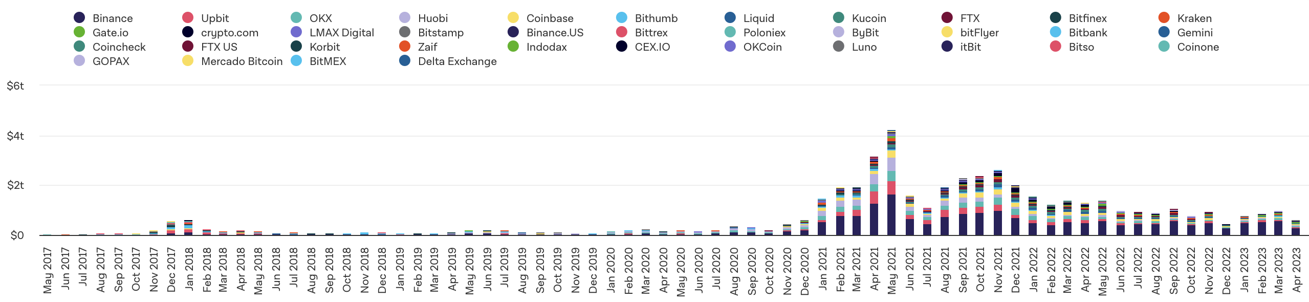
Panel B: DEXs volume

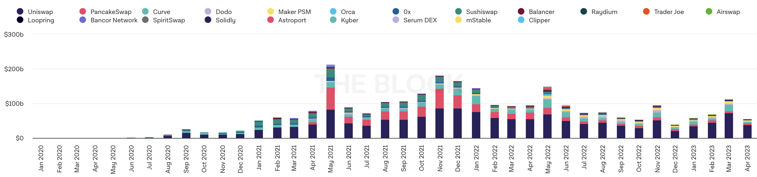
Source: The Block, https://www.theblock.co/data.

Figure 3: Protecting from adverse selection by LPs. Panel A shows a scenario when an LP’s position is adversely selected by an arbitrageur. We assume that ETH price (in USDC) experiences a permanent increase from 1,000 to 2,000. The arbitrageur’s buy trade moves the market price to the new level, depleting all ETH reserves in the LP’s position and leaving him only with USDC. The LP experiences an adverse selection loss of $500K, compared to the scenario, in which he would just hold his initial portfolio of ETH and USDC. Panel B shows that the LP could partially protect himself from adverse selection by redistributing the same amount of capital on a wider price range. Thus, his position would be less concentrated around the market price. Posting on a wider price range would reduce LP’s losses to $300K, because average execution price for his ETH reserves would be higher, compared to Panel A. In contrast, Panel C assumes that the LP continuously monitors the market and is able to update his position even before the arbirtrageur’s trade arrives. In this scenario, the LP is able to fully avoid adverse selection loss and makes a profit of $500K.

Panel A: LP is adversely selected

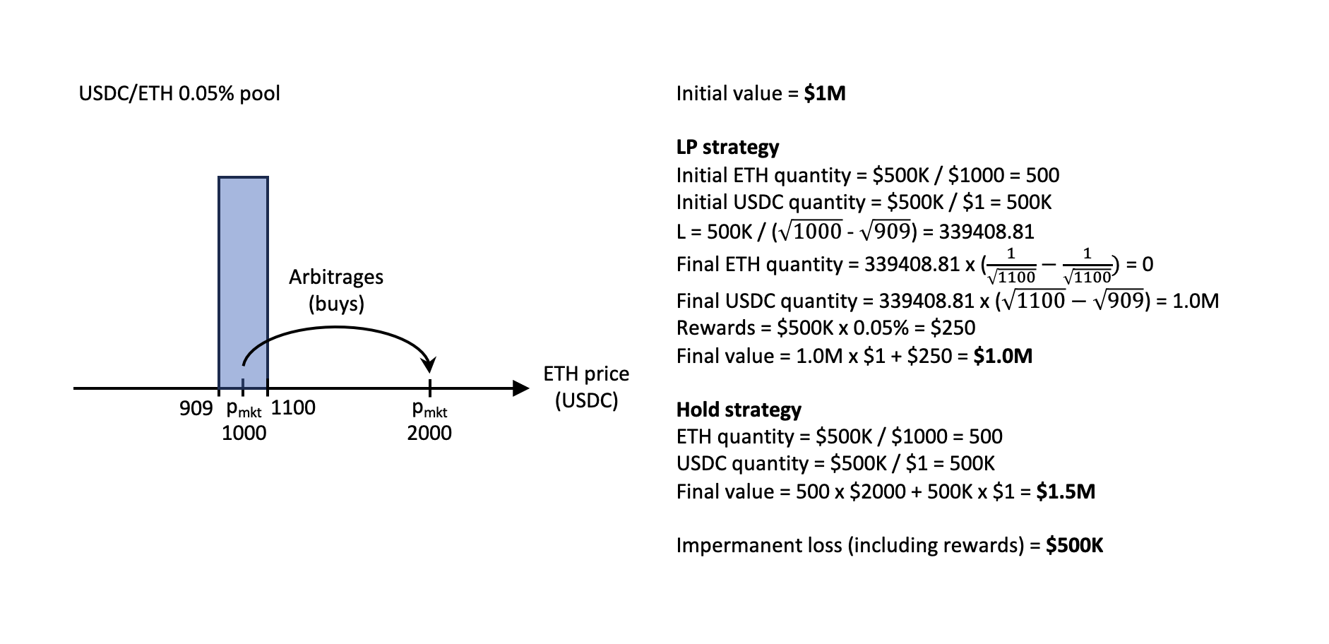
Panel B: Protecting by setting a wider initial price range

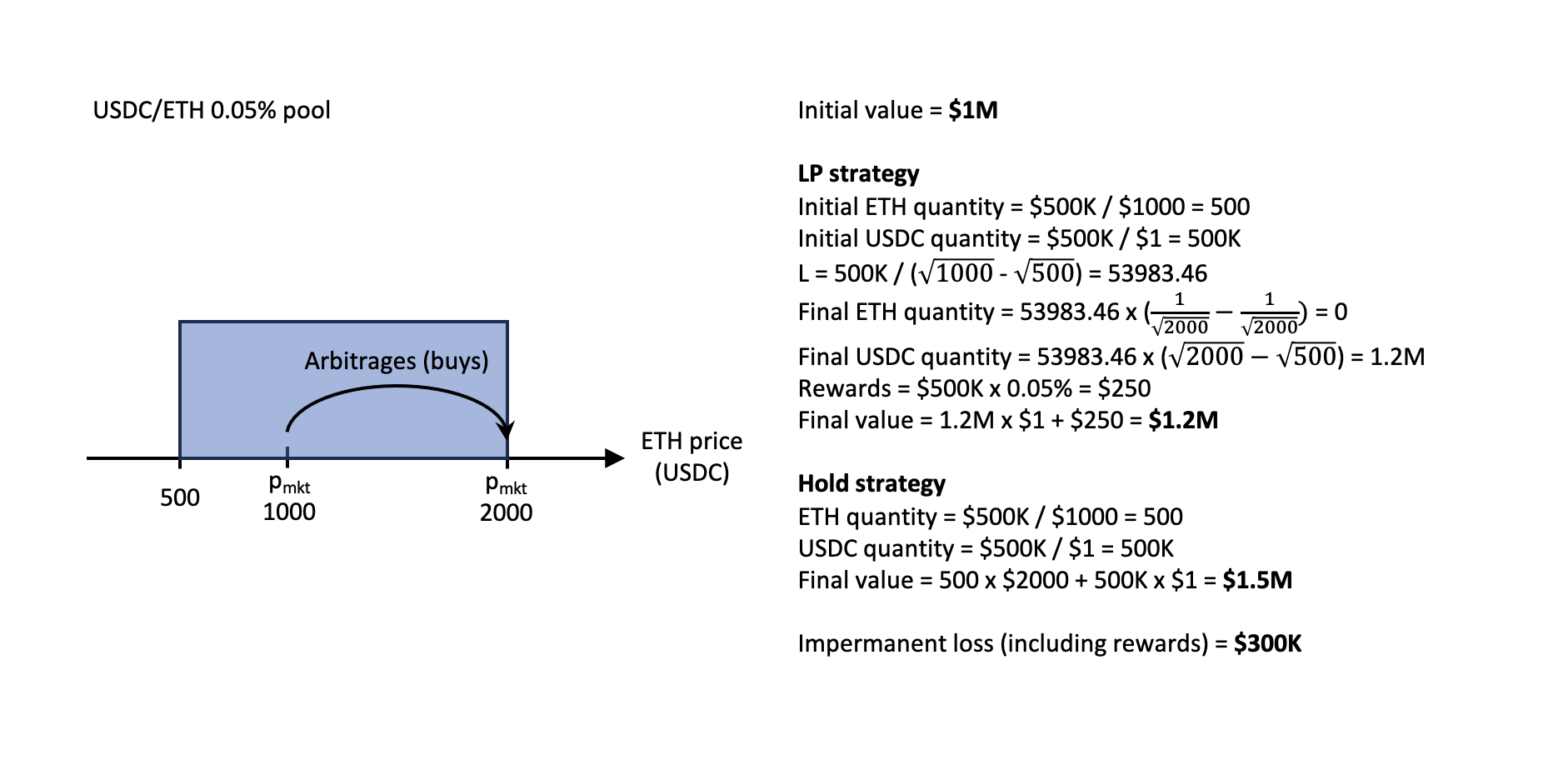
Panel C: Protecting by updating the position

Tables

Table 1: Summary statistics: volume, TVL and trade size. Panel A of this table presents average 24-hour volume (in $M) and average total value locked (TVL) (in $M) on Uniswap v3 across Ethereum, Arbitrum and Polygon for two liquidity pools: ETH/USDC 0.05% and ETH/USDC 0.3%. Panel B reports summary statistics of trade sizes. Panel C reports the average daily numbers of trades, purchases and sales as well as the average time (in seconds) between two trades (delta). Our sample period ranges from January 1, 2022 to June 30, 2023. Appendix E provides a detailed description of all variable definitions.

Panel A: Volume and TVL

Pool	Volume 24h ($M)	TVL ($M)	Volume/TVL
ETH/USDC 0.05%
Ethereum	513.73	201.19	2.55
Arbitrum	51.93	18.04	2.88
Polygon	29.03	10.26	2.83
ETH/USDC 0.3%
Ethereum	57.83	176.59	0.33
Arbitrum	1.65	4.48	0.37
Polygon	0.95	1.89	0.50

Panel B: Trade size

Pool	Mean ($K)	SD	25%	50%	75%
ETH/USDC 0.05%
Ethereum	72.19	255.61	0.82	4.55	42.67
Arbitrum	4.12	10.10	0.06	0.96	4.64
Polygon	2.42	5.09	0.07	0.77	2.86
ETH/USDC 0.3%
Ethereum	116.19	241.02	1.31	30.00	144.65
Arbitrum	2.95	6.76	0.08	1.34	3.33
Polygon	1.74	3.37	0.38	0.88	1.83

Panel C: Trade frequency

Pool	Daily trades	Daily buys	Daily sells	Delta (s)
ETH/USDC 0.05%
Ethereum	7130.90	3495.97	3634.93	12.14
Arbitrum	12668.05	6146.88	6521.17	6.83
Polygon	12048.61	5651.39	6397.23	7.18
ETH/USDC 0.3%
Ethereum	498.17	245.12	253.05	173.75
Arbitrum	560.95	285.41	275.53	154.31
Polygon	545.50	272.64	272.86	158.67

Table 2: Summary statistics: control variables. This table presents summary statistics for the following control variables: the traded volume over the previous 24 hours, $Volume$ (in $M); the realized volatility of ETH/USD over the previous 24 hours, $Volatility$, (in %); and the 1-minute return of ETH/USD, $Return$ (in bp). $Volatility$ and $Return$ are based on a single time series for ETH/USD from Binance, which is independent from Uniswap v3. Appendix E provides a detailed description of all variable definitions. Our sample period ranges from January 1, 2022 to June 30, 2023.

	Mean	SD	25%	50%	75%
Volume 24h ($M)
ETH/USDC 0.05%
Ethereum	513.73	338.53	277.40	466.48	644.16
Arbitrum	51.93	49.65	17.54	33.15	70.16
Polygon	29.03	18.28	16.50	25.52	37.34
ETH/USDC 0.3%
Ethereum	57.83	62.88	17.31	41.96	76.64
Arbitrum	1.65	1.46	0.63	1.08	2.21
Polygon	0.95	0.94	0.30	0.71	1.28
Volatility 24h (%)	3.53	1.87	2.31	3.16	4.26
Return 1min (bp)	0.00	10.53	-3.87	0.00	3.80

Table 3: Liquidity concentration. This table reports average levels of liquidity concentration across Ethereum, Arbitrum and Polygon for two liquidity pools: ETH/USDC 0.05% and ETH/USDC 0.3%. We define liquidity concentration within x% of the market price, as the ratio of market depth within x% of $p_{mkt}$, divided by $TVL$. Market depth within x% of $p_{mkt}$ is computed as the $ value of the liquidity between $\frac{p_{mkt}}{1+x\%}$ and $p_{mkt}\cdot(1+x\%).$ Appendix E provides a detailed description of all variable definitions. Column (1) reports average levels of liquidity concentration within 1% of the market price. Columns (2) and (3) report corresponding statistics for liquidity concentration within 2% and 10% of the market price, respectively. We also report the difference between averages on Arbitrum and Ethereum ($\Delta Arb-Eth$) as well as Polygon and Ethereum ($\Delta Pol-Eth$). T-statistics of the two-tailed t-test with the null-hypothesis of differences equaling zero exceed 100. ***, **, and * indicate statistical significance at the 1%, 5%, and 10% level, respectively.

Pool	Liquidity concentration (%)
	1%		2%		10%
ETH/USDC 0.05%
Ethereum	5.43		10.16		35.28
Arbitrum	6.35		11.85		39.64
$\Delta Arb-Eth$	0.93	***	1.70	***	4.36	***
Polygon	6.61		12.45		42.44
$\Delta Pol-Eth$	1.18	***	2.29	***	7.16	***
ETH/USDC 0.3%
Ethereum	2.80		5.53		24.20
Arbitrum	3.81		7.39		29.56
$\Delta Arb-Eth$	1.01	***	1.85	***	5.36	***
Polygon	5.24		10.20		38.74
$\Delta Pol-Eth$	2.44	***	4.67	***	14.54	***

Table 4: Liquidity provision and repositioning intensity. This table reports average levels of liquidity provision across Ethereum, Arbitrum and Polygon for two liquidity pools: ETH/USDC 0.05% and ETH/USDC 0.3%. We report the average daily number of mints (column 1); the average duration between two mints (in minutes) (column 2); the average daily minted value (in $M) (column 3); the average daily number of burns (column 4); the average duration between two burns (in minutes) (column 5); the average daily burned value (in $M) (column 6); and the average repositioning intensity over 5-minute intervals (in %) (column 7). We define repositioning as a burn followed by a mint in the same pool by the same liquidity provider within next 5 minutes. We measure repositioning intensity as the value of repositioning mints (in $) over a 5-minute interval divided by the total value minted (in $) over the same interval. Appendix E provides a detailed description of all variable definitions. We also report the difference between averages on Arbitrum and Ethereum ($\Delta Arb-Eth$) as well as Polygon and Ethereum ($\Delta Pol-Eth$). T-statistics of the two-tailed t-test with the null-hypothesis of difference equaling zero are reported in parentheses.

Pool	Mints	Delta	Minted	Burns	Delta	Burned	Intensity
	(#/day)	(min)	($M/day)	(#/day)	(min)	($M/day)	(%)
ETH/USDC 0.05%
Ethereum	81.21	17.73	41.19	61.54	23.40	39.90	15.89
Arbitrum	315.27	4.57	11.75	237.83	6.05	11.60	40.64
$\Delta Arb-Eth$	234.06	-13.17	-29.44	176.29	-17.34	-28.31	24.75
	(137.45)		(-29.00)	(106.40)		(-28.19)	(96.64)
Polygon	546.64	2.63	2.95	371.46	3.88	2.82	35.90
$\Delta Pol-Eth$	465.43	-15.10	-38.24	309.92	-19.52	-37.08	20.01
	(246.81)		(-40.04)	(205.67)		(-39.32)	(84.01)
ETH/USDC 0.3%
Ethereum	74.18	19.41	6.53	32.65	44.10	5.42	7.29
Arbitrum	69.92	20.59	0.26	31.66	45.48	0.24	17.10
$\Delta Arb-Eth$	-4.25	1.18	-6.27	-0.99	1.38	-5.18	9.81
	(-4.69)		(-26.33)	(-2.45)		(-22.76)	(36.14)
Polygon	72.94	19.74	0.30	46.88	30.72	0.28	24.78
$\Delta Pol-Eth$	-1.24	0.33	-6.23	14.22	-13.38	-5.14	17.49
	(-1.67)		(-26.16)	(30.70)		(-22.58)	(60.39)

Table 5: Repositioning intensity and liquidity concentration: IV regressions. This table presents results of instrumental variable regressions that test causal effect of repositioning intensity of LPs, $Intensity$, on aggregate liquidity concentration around the market price, $Conc$. Panel A reports results for the low-fee pool (ETH/USDC 0.05%), and Panel B for the high-fee pool (ETH/USDC 0.3%). $Arbitrum$ ($Polygon$) takes value of 1 for Arbitrum (Polygon) pools, and zero for Ethereum pools. Model (1) reports the results for the first-stage regression, with repositioning intensity of LPs, $Intensity$, as the dependent variable and $Arbitrum$ as the main explanatory variable, which is used as an instrument for the endogenous $Intensity$. Model (2) reports results for the second-stage regression, with liquidity concentration within 2% of the market price, $Conc$, as the dependent variable. We estimate liquidity concentration at the end of every 5-minute interval and the repositioning intensity over every 5-minute interval. The set of instruments consists of all explanatory variables, except that $Intensity$ is replaced with $Arbitrum$. The table shows corresponding results for Polygon pools in Models (3) and (4), with $Polygon$ used as an instrument for the endogenous $Intensity$. Models (5) and (6) use $BlockScaling$ that takes value of 1 for both Arbitrum and Polygon pools, and zero for the corresponding Ethereum pool, as an instrument. The vector of control variables consists of $Volume$, $Volatility$ and $|Return|$. See Appendix E for a detailed description of variable definitions. All regressions include hour- and day-fixed effects, with standard errors clustered at the day level. T-statistics of the two-tailed t-test with the null-hypothesis of a coefficient equaling zero are reported in parentheses. ***, **, and * indicate statistical significance at the 1%, 5%, and 10% level, respectively.

Panel A: ETH/USDC 0.05%
	Arbitrum				Polygon				BlockScaling
	Int		Conc		Int		Conc		Int		Conc
			2%				2%				2%
	(1)		(2)		(3)		(4)		(5)		(6)
$Arbitrum$	0.24	***
	(35.55)
$Polygon$					0.20	***
					(33.60)
$BlockScaling$									0.21	***
									(43.78)
$Intensity$			0.09	***			0.11	***			0.11	***
			(59.67)				(66.04)				(69.65)
$Volume$	0.00		0.01	***	-0.01	***	0.01	***	0.01	***	0.01	***
	(1.27)		(48.33)		(-3.42)		(59.75)		(3.85)		(57.25)
$Volatility$	-0.65		-1.52	***	0.45		-1.57	***	-1.35	***	-1.41	***
	(-1.19)		(-41.02)		(1.02)		(-48.61)		(-2.88)		(-51.38)
$|Return|$	23.82	***	-2.98	***	18.11	***	-2.45	***	22.45	***	-3.09	***
	(16.86)		(-27.79)		(17.13)		(-29.57)		(19.14)		(-38.43)
$Observations$	114,817		114,817		148,416		148,416		221,268		221,268
$HourFE$	Yes		Yes		Yes		Yes		Yes		Yes
$DateFE$	Yes		Yes		Yes		Yes		Yes		Yes

Panel B: ETH/USDC 0.3%
	Arbitrum				Polygon				BlockScaling
	Int		Conc		Int		Conc		Int		Conc
			2%				2%				2%
	(1)		(2)		(3)		(4)		(5)		(6)
$Arbitrum$	0.12	***
	(12.57)
$Polygon$					0.16	***
					(28.67)
$BlockScaling$									0.13	***
									(22.40)
$Intensity$			0.08	***			0.22	***			0.15	***
			(29.03)				(40.97)				(43.08)
$Volume$	-0.14	***	0.06	***	-0.00		0.04	***	0.01		0.07	***
	(-3.98)		(42.50)		(-0.19)		(17.74)		(0.53)		(46.28)
$Volatility$	2.97	***	-1.22	***	0.29		-1.08	***	0.32		-1.53	***
	(4.86)		(-39.04)		(0.70)		(-15.60)		(0.70)		(-35.22)
$|Return|$	9.15	***	-0.96	***	17.87	***	-4.15	***	17.49	***	-2.78	***
	(8.47)		(-11.58)		(12.54)		(-18.77)		(13.93)		(-20.79)
$Observations$	53,145		53,145		57,472		57,472		81,810		81,810
$HourFE$	Yes		Yes		Yes		Yes		Yes		Yes
$DateFE$	Yes		Yes		Yes		Yes		Yes		Yes

Table 6: Repositioning intensity and liquidity concentration: robustness checks. This table presents robustness checks for our instrumental variable regressions. Panel A reports results for the low-fee pool (ETH/USDC 0.05%), and Panel B for the high-fee pool (ETH/USDC 0.3%). All models report results of the second-stage IV regressions with $BlockScaling$ as an instrument for $Intensity$, similar to Model (6) in Table 5. $BlockScaling$ takes value of 1 for both Arbitrum and Polygon pools, and zero for the corresponding Ethereum pool. Models (1) and (2) use liquidity concentration within 1% and within 10% of the current market price as the dependent variable, respectively. Model (3) uses an alternative measure for repositioning intensity, $IntensFreq$, defined as the ratio of the number of repositioning mints to the total number of mints within a 5-minute interval. Model (4) uses an alternative measure of $Intensity$, based on the 1-minute repositioning mints. In this analysis, we classify repositioning mints as those that are preceded by burns of the same LP within the previous minute. Model (5) uses 10-minute intervals for estimation of repositioning intensity and liquidity concentration, instead of 5-minute intervals. The vector of control variables consists of $Volume$, $Volatility$ and $|Return|$. See Appendix E for a detailed description of variable definitions. All regressions include hour- and day-fixed effects, with standard errors clustered at the day level. T-statistics of the two-tailed t-test with the null-hypothesis of a coefficient equaling zero are reported in parentheses. ***, **, and * indicate statistical significance at the 1%, 5%, and 10% level, respectively.

Panel A: ETH/USDC 0.05%
	Conc		Conc		IntFreq		Repostn		Aggr
	$1\%$		$10\%$				1-min		10-min
	(1)		(2)		(3)		(4)		(5)
$Intensity$	0.06	***	0.34	***			0.16	***	0.10	***
	(69.57)		(80.57)				(71.87)		(63.62)
$IntensFreq$					0.24	***
					(31.90)
$Volume$	0.00	***	0.02	***	0.01	***	0.01	***	0.01	***
	(57.69)		(47.80)		(33.37)		(69.84)		(53.59)
$Volatility$	-0.84	***	-2.82	***	-1.35	***	-1.44	***	-1.39	***
	(-52.21)		(-36.63)		(-26.90)		(-51.67)		(-45.54)
$|Return|$	-1.85	***	-8.68	***	-6.39	***	-3.71	***	-2.01	***
	(-39.32)		(-37.14)		(-27.97)		(-38.80)		(-32.58)
$Observations$	221,268		221,268		214,875		221,267		149,871
$HourFE$	Yes		Yes		Yes		Yes		Yes
$DateFE$	Yes		Yes		Yes		Yes		Yes

Panel B: ETH/USDC 0.3%
	Conc		Conc		IntFreq		Repostn		Aggr
	$1\%$		$10\%$				1-min		10-min
	(1)		(2)		(3)		(4)		(5)
$Intensity$	0.08	***	0.42	***			0.21	***	0.15	***
	(42.66)		(42.56)				(44.66)		(40.52)
$IntensFreq$					0.17	***
					(37.48)
$Volume$	0.04	***	0.21	***	0.07	***	0.07	***	0.07	***
	(43.93)		(49.60)		(40.42)		(54.16)		(44.07)
$Volatility$	-0.80	***	-4.46	***	-1.52	***	-1.49	***	-1.56	***
	(-33.59)		(-36.66)		(-31.26)		(-35.58)		(-32.65)
$|Return|$	-1.51	***	-7.55	***	-3.33	***	-3.59	***	-2.11	***
	(-20.74)		(-20.20)		(-20.62)		(-21.11)		(-20.42)
$Observations$	81,810		81,810		81,133		81,810		67,874
$HourFE$	Yes		Yes		Yes		Yes		Yes
$DateFE$	Yes		Yes		Yes		Yes		Yes

Table 7: Repositioning precision This table reports average levels of position gap (%), position length (%) and position precision (%) across Ethereum, Arbitrum and Polygon for two liquidity pools: ETH/USDC 0.05% and ETH/USDC 0.3%. We define repositioning gap, $Gap$, as the average gap between the mid price of repositioning mints, $p_{mid}$, and $p_{mkt}$, computed as $\left|\frac{p_{mid}}{p_{mkt}}-1\right|$. $p_{mid}$ is computed as $\sqrt{p_{lower}\cdot p_{upper}}$. We define a repositioning mint as a mint, preceded by a burn in the same pool by the same liquidity provider within previous 5 minutes. Repositioning length, $Length$, is the average range length of repositioning mints, computed as $\frac{\lvert p_{upper}-p_{lower}\rvert}{p_{mid}}$. Repositioning precision, $Precision$, is the average precision of repositioning mints, computed and scaled as $1-1.0001^{\frac{-1}{Gap\cdot Length}}$. Appendix E provides a detailed description of all variable definitions. Column (1) reports average levels of repositioning gap. Columns (2) and (3) report corresponding statistics for repositioning length and repositioning precision, respectively. We also report the difference between averages on Arbitrum and Ethereum ($\Delta Arb-Eth$) as well as Polygon and Ethereum ($\Delta Pol-Eth$). T-statistics of the two-tailed t-test with the null-hypothesis of difference equaling zero are reported in parentheses. ***, **, and * indicate statistical significance at the 1%, 5%, and 10% level, respectively.

Pool	Gap (%)		Length (%)		Precision (%)
ETH/USDC 0.05%
Ethereum	1.86		18.07		50.77
Arbitrum	0.85		10.69		70.89
$\Delta Arb-Eth$	-1.01	***	-7.38	***	20.12	***
	(-49.01)		(-63.20)		(53.98)
Polygon	1.09		12.91		68.60
$\Delta Pol-Eth$	-0.77	***	-5.16	***	17.83	***
	(-32.70)		(-46.43)		(45.23)
ETH/USDC 0.3%
Ethereum	3.41		29.28		20.02
Arbitrum	2.09		15.04		36.63
$\Delta Arb-Eth$	-1.32	***	-14.24	***	16.61	***
	(-17.14)		(-21.76)		(20.50)
Polygon	2.44		15.11		42.12
$\Delta Pol-Eth$	-0.97	***	-14.17	***	22.10	***
	(-12.94)		(-27.87)		(28.70)

Table 8: Repositioning precision and liquidity concentration: IV regressions.This table presents results of instrumental variable regressions that test causal effect of repositioning precision of LPs on liquidity concentration around the market price. We use three measures of repositioning precision: $Gap$, $Length$ and $Precision$. See Appendix E for a detailed description of variable definitions. Panel A reports results for the low-fee pool (ETH/USDC 0.05%), and Panel B for the high-fee pool (ETH/USDC 0.3%). Model (1) reports the results of the first-stage IV regression with $Gap$ as the dependent variable. Model (2) reports the results of the second-stage regression with liquidity concentration within 2% as the dependent variable. $Blockscaling$ is used as an instrument for the endogenous repositioning precision (i.e. $Gap$). Models (3) and (4) present corresponding results for $Length$ as a measure of repositioning precision. Models (5) and (6) present results for $Precision$. The vector of control variables consists of $Volume$, $Volatility$ and $|Return|$. All regressions include hour- and day-fixed effects, with standard errors clustered at the day level. T-statistics of the two-tailed t-test with the null-hypothesis of a coefficient equaling zero are reported in parentheses. ***, **, and * indicate statistical significance at the 1%, 5%, and 10% level, respectively.

Panel A: ETH/USDC 0.05%
	Gap		Conc		Length		Conc		Precision		Conc
			$2\%$				$2\%$				$2\%$
	(1)		(2)		(3)		(4)		(5)		(6)
$BlockScaling$	-0.01	***			-0.05	***			0.12	***
	(-9.26)				(-13.83)				(11.85)
$Gap$			-4.15	***
			(-15.82)
$Length$							-0.47	***
							(-27.70)
$Precision$											0.18	***
											(23.28)
$Volume$	-0.00	***	0.00	***	-0.00	**	0.01	***	0.02	***	0.00	***
	(-5.45)		(7.53)		(-2.56)		(30.86)		(3.76)		(16.52)
$Volatility$	0.26	***	-0.46	***	0.87	***	-1.13	***	-4.65	***	-0.69	***
	(6.02)		(-4.15)		(4.16)		(-21.77)		(-6.21)		(-10.96)
$|Return|$	-0.41	***	-2.28	***	-4.60	***	-2.84	***	6.71	***	-1.77	***
	(-8.99)		(-13.45)		(-13.27)		(-21.15)		(7.66)		(-16.04)
$Observations$	102,625		102,625		102,625		102,625		102,625		102,625
$HourFE$	Yes		Yes		Yes		Yes		Yes		Yes
$DateFE$	Yes		Yes		Yes		Yes		Yes		Yes

Panel B: ETH/USDC 0.3%
	Gap		Conc		Length		Conc		Precision		Conc
			$2\%$				$2\%$				$2\%$
	(1)		(2)		(3)		(4)		(5)		(6)
$BlockScaling$	-0.01	***			-0.11	***			0.12	***
	(-5.01)				(-13.11)				(8.84)
$Gap$			-3.05	***
			(-7.05)
$Length$							-0.16	***
							(-17.55)
$Precision$											0.15	***
											(15.52)
$Volume$	-0.01	***	0.04	***	-0.04	**	0.06	***	0.15	***	0.04	***
	(-3.31)		(5.73)		(-2.10)		(23.71)		(5.42)		(11.82)
$Volatility$	0.27	***	-0.74	***	1.36	***	-1.34	***	-5.42	***	-0.72	***
	(2.84)		(-3.09)		(3.13)		(-17.31)		(-6.55)		(-6.48)
$|Return|$	-0.25	**	-0.80	***	-3.53	***	-0.62	***	7.60	***	-1.21	***
	(-2.58)		(-2.74)		(-6.67)		(-5.88)		(7.43)		(-7.36)
$Observations$	15,173		15,174		15,173		15,174		15,173		15,174
$HourFE$	Yes		Yes		Yes		Yes		Yes		Yes
$DateFE$	Yes		Yes		Yes		Yes		Yes		Yes

Table 9: Slippage: summary statistics and multivariate analysis. Panel A of this table presents summary statistics for slippage, $Slippage$ (in bp), on Uniswap v3 across Ethereum, Arbitrum and Polygon for two liquidity pools: ETH/USDC 0.05% and ETH/USDC 0.3%. We compute $Slippage$ for hypothetical trades of sizes [$100, $500, $1K, $5K, $10K, $50K, $100K] for every minute in our sample period (January 1, 2022 - June 30, 2023). Panels B and C present the results of OLS regressions with slippage, $Slippage$ (in bp), as the dependent variable. Model (1) reports the results for the total sample, with $BlockScaling$ equal to 1 for hypothetical trades on Arbitrum and Polygon, and zero otherwise. Trades on Ethereum represent the benchmark sample. Models (2) and (3) report results, conditioning on the trade size. Specifically, we define $Large$ equal to 1 if a trade exceeds $1K (Model 2) or $5K (Model 3), and zero otherwise. Models (4) and (5) report results for the benchmark Model (2), separately for Arbitrum and Polygon. The vector of control variables consists of $Size$, $Buy$, $Volume$, $Volatility$, $|Return|$. See Appendix E for a detailed description of variable definitions. All regressions include hour- and date-fixed effects, with standard errors clustered at the day level. T-statistics of the two-tailed t-test with the null-hypothesis of a coefficient equaling zero are reported in parentheses. ***, **, and * indicate statistical significance at the 1%, 5%, and 10% level, respectively.

Panel A: Summary statistics
	Mean	SD	25%	50%	75%
Slippage (bp)
ETH/USDC 0.05%
Ethereum	0.30	0.61	0.01	0.05	0.37
Arbitrum	8.80	27.81	0.07	0.60	4.25
Polygon	4.25	8.05	0.09	0.73	5.92
ETH/USDC 0.3%
Ethereum	0.55	0.90	0.01	0.11	0.85
Arbitrum	23.25	51.95	0.35	2.62	20.63
Polygon	34.24	62.18	0.72	5.40	38.23

Panel B: ETH/USDC 0.05%
	BlockScaling						Arbitrum		Polygon
	Total		Large $>\$1K$		Large $>\$5K$		Large $>\$1K$		Large $>\$1K$
	(1)		(2)		(3)		(4)		(5)
$BlockScaling$	1.41	***	-4.60	***	-4.32	***
	(3.18)		(-9.10)		(-8.65)
$Arbitrum$							-6.41	***
							(-8.09)
$Polygon$									-1.62	***
									(-8.73)
$BlockSc\cdot Large$			10.53	***	13.37	***	14.37	***	6.67	***
			(19.79)		(19.79)		(15.12)		(42.59)
$Large$			0.51	***	0.65	***	0.51	***	0.51	***
			(37.00)		(37.00)		(37.00)		(37.00)
$Size$	0.19	***
	(20.63)
$Buy$	-0.00		-0.00		-0.00		0.01		-0.01	***
	(-0.22)		(-0.22)		(-0.22)		(0.27)		(-3.42)
$Volume$	-0.01	***	-0.01	***	-0.01	***	-0.01	***	-0.00	***
	(-9.06)		(-9.06)		(-9.06)		(-8.02)		(-9.61)
$Volatility$	0.86	***	0.86	***	0.86	***	1.38	***	0.41	***
	(8.96)		(8.96)		(8.96)		(7.68)		(9.33)
$|Return|$	0.48	***	0.48	***	0.48	***	0.39	***	0.33	***
	(9.26)		(9.26)		(9.26)		(5.83)		(10.60)
$R^{2}$	0.28		0.20		0.24		0.24		0.36
$Observations$	6,603,702		6,603,702		6,603,702		4,402,468		4,402,468
$HourFE$	Yes		Yes		Yes		Yes		Yes
$DateFE$	Yes		Yes		Yes		Yes		Yes

Panel C: ETH/USDC 0.3%
	BlockScaling						Arbitrum		Polygon
	Total		Large $>\$1K$		Large $>\$5K$		Large $>\$1K$		Large $>\$1K$
	(1)		(2)		(3)		(4)		(5)
$BlockScaling$	21.61	***	-5.78	***	-4.48	***
	(31.41)		(-8.00)		(-6.29)
$Arbitrum$							-9.74	***
							(-12.45)
$Polygon$									-1.07
									(-1.20)
$BlockSc\cdot Large$			47.94	***	60.89	***	38.50	***	57.38	***
			(50.21)		(50.17)		(29.78)		(43.93)
$Large$			0.94	***	1.19	***	0.94	***	0.94	***
			(68.44)		(68.45)		(68.44)		(68.44)
$Size$	0.81	***
	(51.08)
$Buy$	0.18	*	0.18	*	0.18	*	0.29	***	-0.03
	(1.68)		(1.68)		(1.68)		(3.22)		(-0.25)
$Volume$	-0.12	***	-0.12	***	-0.12	***	-0.19	***	-0.03	**
	(-9.32)		(-9.32)		(-9.32)		(-12.40)		(-2.09)
$Volatility$	2.11	***	2.11	***	2.11	***	3.20	***	1.27	***
	(10.90)		(10.90)		(10.90)		(11.57)		(4.50)
$|Return|$	1.00	***	1.00	***	1.00	***	0.51	***	0.98	***
	(6.63)		(6.63)		(6.63)		(2.89)		(8.19)
$R^{2}$	0.49		0.30		0.41		0.34		0.36
$Observations$	6,603,702		6,603,702		6,603,702		4,402,468		4,402,468
$HourFE$	Yes		Yes		Yes		Yes		Yes
$DateFE$	Yes		Yes		Yes		Yes		Yes

Table 10: Repositioning and liquidity concentration: Arbitrum airdrop. This table presents results of instrumental variable regressions that test causal effect of repositioning intensity and precision, separately before and after the airdrop of ARB token on March 23, 2023. Panel A reports results for the low-fee pool (ETH/USDC 0.05%), and Panel B for the high-fee pool (ETH/USDC 0.3%). Models (1)-(3) report results for the pre-airdrop sample, and Models (4)-(6) for the post-airdrop sample. Models (1) and (4) report the results for the first-stage regression, with repositioning intensity of LPs, $Intensity$, as the dependent variable and $Arbitrum$ as the main explanatory variable, which is used as an instrument for the endogenous $Intensity$. $Arbitrum$ takes value of 1 for Arbitrum pools, and zero for Ethereum pools. Models (2) and (5) report results for the second-stage regression, with liquidity concentration within 2% of the market price, $Conc$, as the dependent variable. We estimate liquidity concentration at the end of every 5-minute interval and the repositioning intensity over the previous 5-minute interval. The set of instruments consists of all explanatory variables, except that $Intensity$ is replaced with $Arbitrum$. Models (3) and (6) report results for the second-stage regressions, with $Arbitrum$ used as an instrument for the endogenous $Precision$. The vector of control variables consists of $Volume$, $Volatility$ and $|Return|$. See Appendix E for a detailed description of variable definitions. All regressions include hour- and day-fixed effects, with standard errors clustered at the day level. T-statistics of the two-tailed t-test with the null-hypothesis of a coefficient equaling zero are reported in parentheses. ***, **, and * indicate statistical significance at the 1%, 5%, and 10% level, respectively.

Panel A: ETH/USDC 0.05%
	Before Airdrop						After Airdrop
	Int		Conc		Conc		Int		Conc		Conc
			$2\%$		$2\%$				$2\%$		$2\%$
	(1)		(2)		(3)		(4)		(5)		(6)
$Arbitrum$	0.22	***					0.35	***
	(31.23)						(17.93)
$Intensity$			0.04	***					0.29	***
			(29.71)						(35.37)
$Precision$					0.05	***					0.68	***
					(13.90)						(7.11)
$Volume$	0.00		0.01	***	0.01	***	-0.03	**	0.01	***	-0.00
	(1.17)		(53.87)		(28.77)		(-2.59)		(6.59)		(-0.53)
$Volatility$	-0.90		-1.30	***	-1.22	***	5.74	***	-3.34	***	3.07	**
	(-1.56)		(-47.41)		(-27.48)		(3.28)		(-12.26)		(2.05)
$|Return|$	24.24	***	-1.57	***	-0.64	***	20.11	***	-6.55	***	-6.67	***
	(15.58)		(-21.40)		(-9.10)		(6.88)		(-10.33)		(-4.74)
$Observations$	87,698		87,698		33,849		27,119		27,119		14,138
$HourFE$	Yes		Yes		Yes		Yes		Yes		Yes
$DateFE$	Yes		Yes		Yes		Yes		Yes		Yes

Panel B: ETH/USDC 0.3%
	Before Airdrop						After Airdrop
	Int		Conc		Conc		Int		Conc		Conc
			$2\%$		$2\%$				$2\%$		$2\%$
	(1)		(2)		(3)		(4)		(5)		(6)
$Arbitrum$	0.07	***					0.12	***
	(2.74)						(12.25)
$Intensity$			0.07	***					0.65	***
			(27.16)						(3.69)
$Precision$					0.06	***					0.31	**
					(7.04)						(2.37)
$Volume$	-0.15	***	0.06	***	0.04	***	0.20		-0.08		-0.04
	(-4.08)		(44.17)		(11.10)		(1.57)		(-0.92)		(-0.54)
$Volatility$	3.09	***	-1.15	***	-0.63	***	-1.03		-0.59		0.00
	(4.93)		(-41.39)		(-7.54)		(-0.28)		(-0.31)		(.)
$|Return|$	8.90	***	-0.81	***	-0.34	***	15.63	***	-10.37	**	0.79
	(8.10)		(-11.25)		(-3.71)		(3.81)		(-2.57)		(0.50)
$Observations$	49,943		49,943		6,604		3,202		3,202		549
$HourFE$	Yes		Yes		Yes		Yes		Yes		Yes
$DateFE$	Yes		Yes		Yes		Yes		Yes		Yes

Appendix A

Estimating gas fees

Any transaction on a blockchain requires the payment of gas fees, which are used to compensate validators for their work in verifying transactions and securing the network.

Gas fees are computed with the quantity of gas units required, which depends on the transaction. For example, a trade on Uniswap v3 (Ethereum) requires on average 120K gas units.

The price of one gas unit, the gas price, varies over our sample period, as shown in Panel A of Figure A1. Panel B shows the gas fees to pay for a hypothetical trade on Uniswap v3 (Ethereum) that requires 120K gas units. These fees vary from as little as $1.30 in October 2022 to $160 during the period of Terra collapse in early May 2022. On average, a trade that requires 120K gas units on Uniswap v3 (Ethereum) costs $14 in gas fees in 2022.

Figure A1: Gas price and gas fees on Ethereum. Panel A of this figure shows historical gas price on Ethereum over 2022, downloaded from Etherscan. Panel B shows gas fees for a trade on Uniswap v3 (Ethereum), assuming that it requires on average 120K gas units.

Panel A

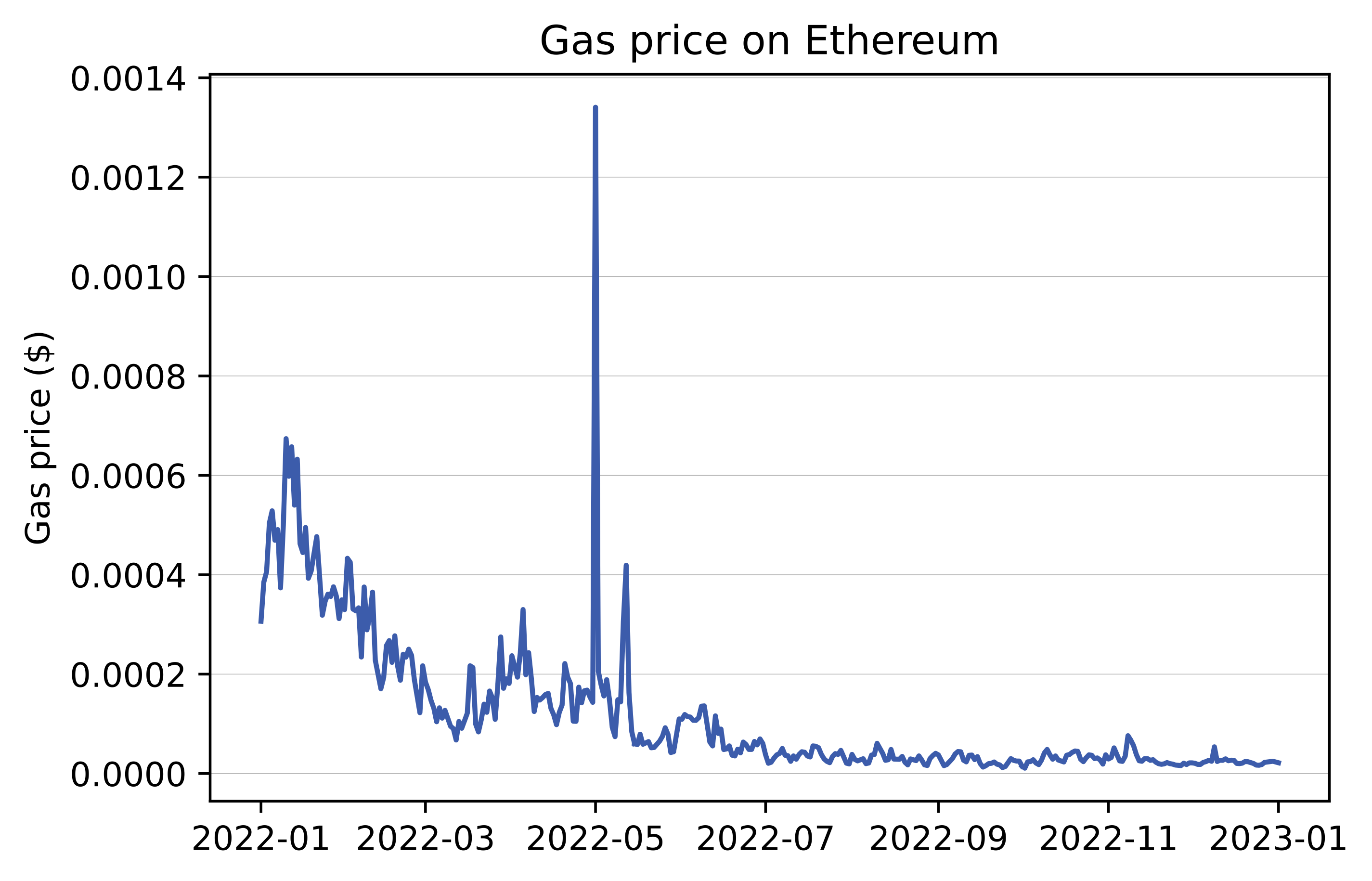
Panel B

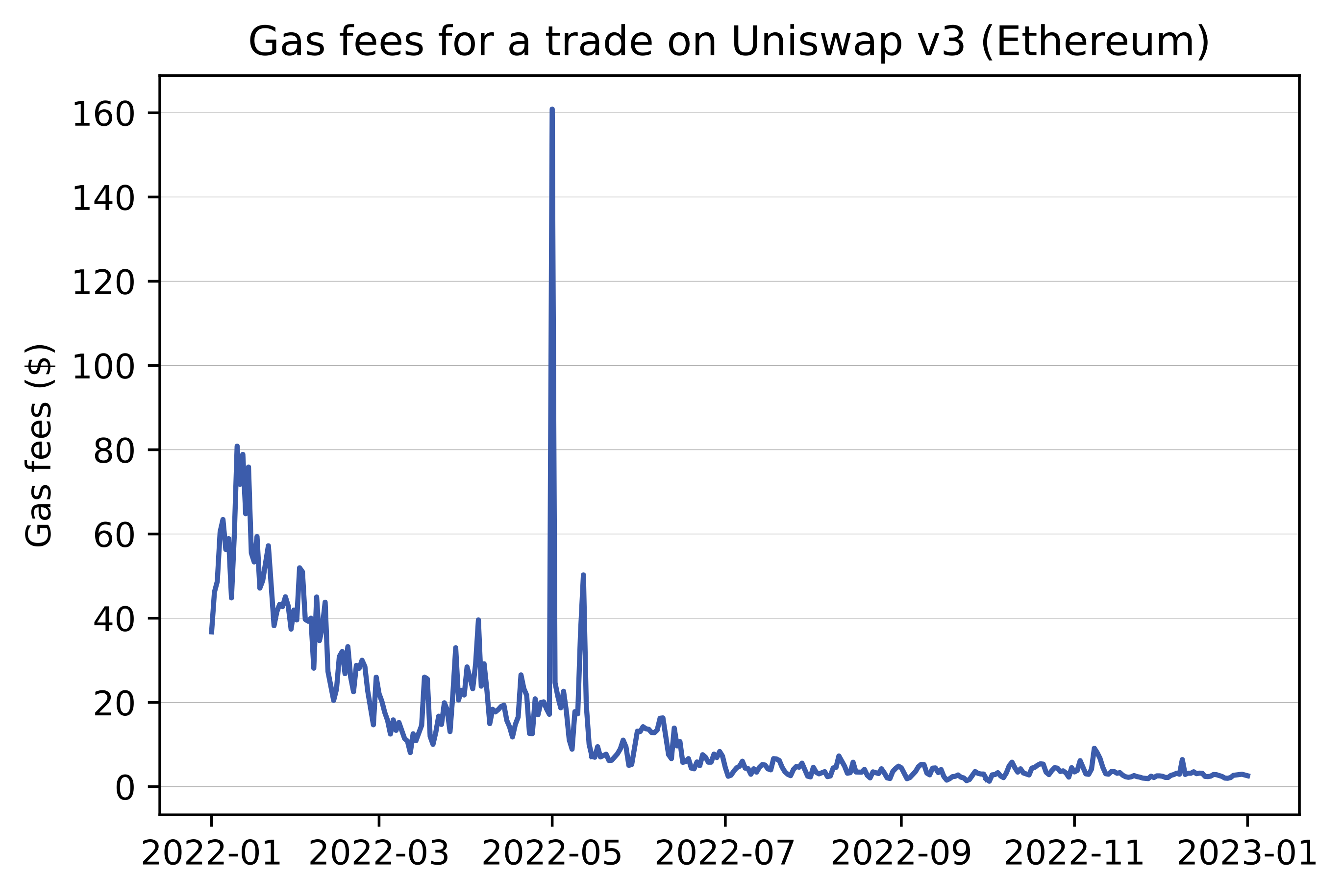
Appendix B

Trading mechanics on Uniswap v2 and Uniswap v3

Uniswap v2. Uniswap v2 is a constant product market maker (CPMM), which is a widely adopted subclass of automated market makers (AMMs). The price curve, or so-called bonding curve, is defined as:

$$x\cdot y=k$$ (2)

where $x$ is the current quantity of token X, the base token (e.g., BTC for BTC/USDT pair), $y$ is the current quantity of token Y, the quote token (e.g., USDT for BTC/USDT pair) and $k$ is the pool’s constant, showing the total liquidity available in the pool. In absence of mints and burns, pool’s constant $k$ has to preserve its value. For example, a trade (or swap) that buys BTC with USDT will remove $\triangle x$ of BTC from the pool and add $\triangle y$ of USDT to the pool. Denote the new amount of BTC in the pool after the trade as $x^{\prime}$, i.e. $x^{\prime}=x+\triangle x$, and the new amount of USDT as $y^{\prime}$, i.e. $y^{\prime}=y+\triangle y,$ with $\triangle x<0$ and $\triangle y>0$. CPMM requires $k$ to be the same before and after the trade:

$$x\cdot y=(x+\triangle x)(y+\triangle y)=k$$ (3)

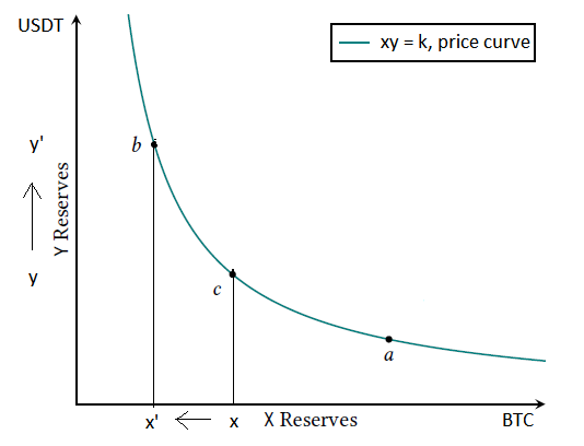
Figure A2: Price curve for Uniswap v2: constant product market maker (CPMM). This figure illustrates a swap on the BTC/USDT pool on Uniswap v2. Pool reserves of token X, i.e. BTC, are on the x-axis. Pool reserves of token Y, i.e. USDT, are on y-axis. The price curve, $x\cdot y=k$, ensures the constant product between the reserves of the pool’s two assets (in absence of liquidity deposits/withdrawals). A buy of BTC with USDT reduces the reserves of BTC from $x$ to $x^{\prime}$ and increases the reserves of USDT from $y$ to $y^{\prime}.$ The pool price after the buy moves upwards from $p_{c}$ to $p_{b}.$

Therefore, the product between the reserves of the pool’s two tokens is constant, provided there is no changes to total liquidity in the pool. Figure A2 illustrates this trade as a transition along the price curve from state $c$ to state $b$. Note that the convexity of the curve causes the trader to receive less BTC than the actual BTC value of the USDT added to the pool, i.e. slippage of the trade is determined by convexity of the price curve.

[Insert Figure A2 approximately here]

The market price in Uniswap v2 pools is determined by the ratio of the current quantities of two tokens in the pool:

$$p_{mkt}=\frac{y}{x}$$ (4)

which shows the market price of token X (BTC) in units of token Y (USDT). After the trade, as in example above, price of BTC increases to $p^{\prime}_{mkt}=\frac{y^{\prime}}{x^{\prime}}$, because removing some of BTC from the pool makes it relatively scarce. In contrast, adding USDT to the pool makes it a relatively abundant asset, such that it becomes relatively cheaper.

In Uniswap v2, LPs are required to deposit their liquidity in a 50-50 ratio, i.e. they deposit both tokens in equivalent quantities. If liquidity providers add liquidity to the pool, the pool size increases, i.e. the pool’s constant $k$ increases. The larger the pool size the lower the slippage of a given trade. However, trading fees are then shared between a larger number of LPs. Recent studies by [6], [15], and [9] discuss the economics of Uniswap v2 in more detail. Specifically, they show that LPs face a trade-off between the amount of fees earned from liquidity providing and adverse selection cost, imposed on them by informed arbitrageurs. [15] and [9] further show that the pool size acts as an equilibrating mechanism on DEXs, equivalent to the bid-ask spread on CEXs.

Uniswap v3. In Uniswap v2, liquidity deposited in the pool is uniformly distributed along the price curve, i.e. it is available for trading on the entire price range, $[0,\infty[$. The advantage of this traditional implementation of AMM is that LPs earn fees irrespective of the market price. However, it requires a great amount of capital to be “locked up” in the pool without being “active”, i.e. used in swaps. For example, prices close to infinity are definitely unrealistic, but the same amount of liquidity is reserved at these unrealistic prices than at the market price.

Uniswap v3 seeks to improve “capital efficiency” of liquidity providers, by allowing them to “concentrate” their liquidity on smaller price ranges. When they open a new liquidity position, i.e. deposit their tokens to a Uniswap v3 pool, they have to specify a price range, $[p_{a},p_{b}]$, where $p_{a}$ is the minimum price and $p_{b}$ the maximum price of token X in units of token Y at which their position is active. According to Uniswap v3 whitepaper [1], “a position only needs to maintain enough reserves to support trading within its range, and therefore can act like a constant product pool with larger (virtual) reserves within that range”.

Figure A3 illustrates the notion of “virtual reserves”. A position on a range of $[p_{a},p_{b}]$ and a market price $p_{c}\in[p_{a},p_{b}]$ only needs to hold a smaller amount of real X reserves, $x_{real}$, which are gradually depleted (i.e. swapped against Y reserves) until the market price, $p_{c}$, reaches the upper price bound, $p_{b}$. If the market price reaches $p_{b}$, then all X reserves are depleted and the position is no longer active, i.e. stops earning fees. The position then consists only of Y reserves. Similarly, this position only needs to hold $y_{real}$ reserves, which are gradually depleted until the market price reaches the lower price bound, $p_{a}$, when Y reserves are depleted and the position becomes inactive. Should the pool price fall back to the specified price range, the liquidity position becomes active again. Thus, virtual reserves ($x$ and $y$) magnify real reserves ($x_{real}$ and $y_{real}$) in a way that the liquidity in the pool matches that of the market price range.

[Insert Figure A3 approximately here]

The price curve for Uniswap v3 is a modification of $x\cdot y=k$, such that the position is solvent exactly within its price range, $[p_{lower},p_{upper}]$ [1]:

$$\left(x+\frac{L}{\sqrt{p_{upper}}}\right)\left(y+L\sqrt{p_{lower}}\right)=L^{2},$$ (5)

where $x$ and $y$ represent virtual reserves, and $L$ is a “liquidity” constant that shows the amount of liquidity deposited for each position.

In contrast to Uniswap v2, the amount of tokens deposited in a liquidity position is no longer in 50-50 ratio. In fact, it depends on the selected price range relative to the market price, with larger reserves of Y required if the price range is skewed to prices lower than the market price, $p_{mkt}$. If the selected price range is strictly lower than the market price (and excludes it), then LP only has to deposit token Y. This case corresponds to point $b$ being below point $c$ on the price curve on Figure A3, i.e. $p_{mkt}>[p_{lower},p_{upper}]$. Similarly, if the preferred price range is strictly higher than the market price, then LP only has to deposit token X. This case corresponds to point $a$ being above point $c$ on Figure A3, i.e. $p_{mkt}<[p_{lower},p_{upper}]$.

Adding liquidity to Uniswap v3 pools. On Uniswap v3, LPs are able to specify the price range on which their liquidity position will be active. To make this possible, the space of prices is divided into discrete ticks, [$i$, $i\in\mathbb{Z}$]. According to Uniswap v3 whitepaper [1], there can be a tick at every price that is an integer power of 1.0001, such that the following relation holds for the price $p_{i}$ corresponding to tick $i$:

$$p_{i}=1.0001^{i}$$ (6)

Specifically, this relation implies that each tick is 1 bp (basis point) away from its neighbouring ticks. However, not all ticks can be initialized, but only those that are divisible by a pre-specified pool parameter, the tick spacing $s$. For example, USDC/ETH 0.3% pool has a $s$ of 60. Therefore, only ticks that are divisible by 60 can be initialized, i.e. (-120, -60, 0, 60, 120…). A tick range can then be defined as $[i,i+s]$.

One liquidity position of an LP can cover one or more tick ranges, $[i,i+s]$. The liquidity on each tick range $[i,i+s]$, $L_{i}$, is then an aggregation of all LP positions that are currently active on it. Therefore, aggregated liquidity in a Uniswap v3 pool is no longer constant (as in Uniswap v2), but fragmented across multiple tick ranges. Figure A4 illustrates a stylized distribution of liquidity on the price space for Uniswap v2 and Uniswap v3 [1].

[Insert Figure A4 approximately here]

Let $p_{i}$ denote the price of token X (in units of token Y) that corresponds to tick $i$. From Uniswap v3 whitepaper [1], we obtain the following relations for $x_{i}$, quantity of tokens X locked in the tick range $[i,i+s]$, and $y_{i},$ quantity of tokens Y locked in the same tick range:

$$x_{i}=\frac{L_{i}}{\sqrt{z_{i}}}-\frac{L_{i}}{\sqrt{p_{i+s}}}$$ (7)

$$y_{i}=L_{i}\cdot(\sqrt{z_{i}}-\sqrt{p_{i}})$$ (8)

where

$$p_{i}\text{ if }p_{mkt}\leq p_{i}$$

$$p_{mkt}\text{ if }p_{i}<p_{mkt}<p_{i+s}$$

$$p_{i+s}\text{ if }p_{i+s}\leq p_{mkt}$$

Appendix D provides a numerical example of adding liquidity to USDC/ETH 0.3% pool.

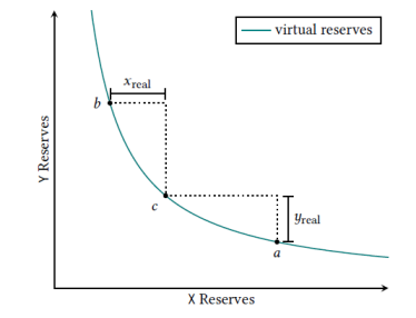
Figure A3: Price curve for Uniswap v3: constant product market maker (CPMM) with virtual reserves. This figure illustrates the virtual reserves curve on Uniswap v3. A position on a range of $[p_{a},p_{b}]$ and a market price $p_{c}\in[p_{a},p_{b}]$ only needs to hold a smaller amount of real X reserves, $x_{real}$, which are gradually depleted (i.e. swapped against Y reserves) until the market price, $p_{c}$, reaches the upper price bound, $p_{b}$. If the market price reaches $p_{b}$, then all X reserves are depleted and the position is no longer active, i.e. stops earning fees. The position then consists only of Y reserves. Similarly, this position only needs to hold $y_{real}$ reserves, which are gradually depleted until the market price reaches the lower price bound, $p_{a}$, when Y reserves are depleted and the position becomes inactive.

Source: Uniswap v3 whitepaper

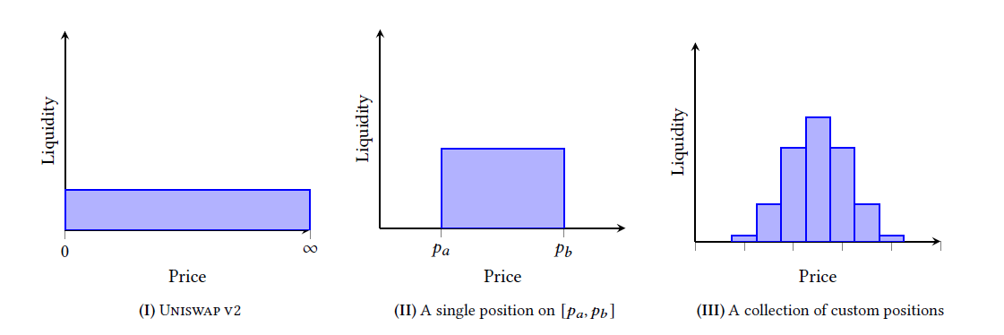
Figure A4: Examples of liquidity distributions on the price space. Panel (I) shows that liquidity distribution in Uniswap v2 is constant on the entire price range. Panel (II) shows an example of a single position of a liquidity provider on Uniswap v3 with the specified price range $[p_{lower},p_{upper}].$ Again, liquidity provided is constant within the price range of this position. This price range can cover one or more tick ranges $[i,i+s].$ Panel (III) shows fragmentation of liquidity across multiple tick ranges on Uniswap v3. Liquidity within each tick range is constant and represents an aggregation of all LP positions active on this tick range.

Source: [1].

Appendix C

Trading on Uniswap v3

Trading on Uniswap v3 within a given tick range. Suppose we would like to submit a trade to USDC/ETH 0.3% pool, i.e. swap tokens X and tokens Y. Let $\triangle x$ and $\triangle y$ denote the total quantities of tokens X and Y to be swapped in a trade (for example, if we would like to buy tokens X with tokens Y, we have $\triangle x<0$ and $\triangle y>0$). Since liquidity is fragmented along tick ranges, we have to consider separately every tick range that is necessary for trade execution. Let $\triangle x_{i}$ and $\triangle y_{i}$ denote the quantities of tokens X and Y to be swapped within a given tick range $[i,i+s]$. Price curve in Equation (5) imposes:

$$\left(x_{i}+\triangle x_{i}+\frac{L_{i}}{\sqrt{p_{i+s}}}\right)\cdot\left(y_{i}+\triangle y_{i}+L_{i}\cdot\sqrt{p_{i}}\right)=\left(x_{i}+\frac{L_{i}}{\sqrt{p_{i+s}}}\right)\cdot\left(y_{i}+L_{i}\cdot\sqrt{p_{i}}\right)=L_{i}^{2}$$ (9)

from where we obtain the following for $\triangle x_{i}$ and $\triangle y_{i}$:

$$\Rightarrow\begin{cases}\triangle x_{i}=-\frac{\triangle y_{i}\cdot(x_{i}+\frac{L_{i}}{\sqrt{p_{i+s}}})}{y_{i}+\triangle y_{i}+L_{i}\cdot\sqrt{p_{i}}}\\ \triangle y_{i}=-\frac{\triangle x_{i}\cdot(y_{i}+L_{i}\cdot\sqrt{p_{i}})}{x_{i}+\triangle x_{i}+\frac{L_{i}}{\sqrt{p_{i+s}}}}\end{cases}$$ (10)

Tick-crossing trades on Uniswap v3. Below we provide general formulas for trades that are too large to be executed within a single tick range and involve crossing several ticks. Suppose we would like to sell tokens X (USDC) for tokens Y (ETH). We are adding $\triangle x>0$ to the pool and withdrawing $\triangle y<0$.

For a given tick range $[i,i+s]$, denote by $\triangle x_{i}^{max}$ the maximum quantity of tokens X that you can add to this range (by taking reserves of token Y). Let $\triangle y_{i}^{min}$ denote the minimum quantity of tokens Y that you can “add” to this range - or, in other words, the maximum quantity of tokens Y than you can take from this range by adding tokens X. From liquidity distribution of the pool, we know reserves $y_{i}$ for each tick range, such that $\triangle y_{i}^{min}=-y_{i}$. We can then compute $\triangle x_{i}^{max}$ using Equation (10):

$$\triangle y_{i}^{min}=-y_{i}$$

$$\triangle x_{i}^{max}=-\frac{\triangle y_{i}^{min}\cdot(x_{i}+\frac{L_{i}}{\sqrt{p_{i+s}}})}{y_{i}+\triangle y_{i}^{min}+L_{i}\cdot\sqrt{p_{i}}}=\frac{x_{i}y_{i}}{L_{i}\cdot\sqrt{p_{i}}}+\frac{y_{i}}{\sqrt{p_{i}p_{i+s}}}$$

Let $\{i_{start},i_{start}-s,...,i_{end}\}$ be the lower ticks of the consecutive tick ranges that we use during the trade. We consume all available liquidity in the tick ranges of lower ticks $i\in\{i_{start},i_{start}-s,...,i_{end}+s\}$, and spend our remaining tokens X in the tick range of lower tick $i_{end}$, such that $\triangle x$ and $\triangle y$ can be expressed as follows:

$$\triangle x=\sum_{i\in\{i_{start},i_{start}-s,...,i_{end}+s\}}\triangle x_{i}^{max}+\triangle x_{i_{end}}$$

$$\triangle y=\sum_{i\in\{i_{start},i_{start}-s,...,i_{end}+s\}}\triangle y_{i}^{min}+\triangle y_{i_{end}}$$

$$\Rightarrow\boxed{\begin{cases}\triangle x_{i_{end}}=\triangle x-\sum_{i\in\{i_{start},i_{start}-s,...,i_{end}+s\}}\triangle x_{i}^{max}\\ \triangle y\overset{(\ref{eq:delta_xy})}{=}-\sum_{i\in\{i_{start},i_{start}-s,...,i_{end}+s\}}y_{i}-\frac{\triangle x_{i_{end}}\cdot(y_{i_{end}}+L_{i_{end}}\cdot\sqrt{p_{i_{end}}})}{x_{i_{end}}+\triangle x_{i_{end}}+\frac{L_{i_{end}}}{\sqrt{p_{i_{end}+s}}}}\end{cases}}$$ (11)

Appendix D provides numerical examples of calculating slippage for trades within the current market range and for tick-crossing trades. Below we also provide formulas for the opposite trade direction, i.e. buying X with Y.

Opposite trade direction: buy X with Y. Suppose we would like to buy tokens X with tokens Y. We are adding $\triangle y>0$ to the pool and removing $\triangle x<0$.

For a given tick range $[i,i+s]$, denote by $\triangle y_{i}^{max}$ the maximum quantity of tokens Y that you can add to this range (by removing reserves of token X). Let $\triangle x_{i}^{min}$ denote the minimum quantity of tokens X that you can “add” to this range, i.e. the maximum quantity of tokens X than you can take from this range by adding tokens Y. From liquidity distribution of the pool, we know reserves $x_{i}$ for each tick range, such that $\triangle x_{i}^{min}=-x_{i}$. We can then compute $\triangle y_{i}^{max}$ using Equation (10):

$$\triangle x_{i}^{min}=-x_{i}$$

$$\triangle y_{i}^{max}=-\frac{\triangle x_{i}^{min}\cdot(y_{i}+L_{i}\cdot\sqrt{p_{i}})}{x_{i}+\triangle x_{i}^{min}+\frac{L_{i}}{\sqrt{p_{i+s}}}}=\frac{x_{i}y_{i}\sqrt{p_{i+s}}}{L_{i}}+x_{i}\cdot\sqrt{p_{i}p_{i+s}}$$

Let $\{i_{start},i_{start}+s,...,i_{end}\}$ be the lower ticks of the consecutive tick ranges that we use during the trade. We consume all available liquidity in the tick ranges of lower ticks $i\in\{i_{start},i_{start}+s,...,i_{end}-s\}$, and spend our remaining tokens Y in the tick range of lower tick $i_{end}$, such that $\triangle x$ and $\triangle y$ can be expressed as follows:

$$\triangle y=\sum_{i\in\{i_{start},i_{start}+s,...,i_{end}-s\}}\triangle y_{i}^{max}+\triangle y_{i_{end}}$$

$$\triangle x=\sum_{i\in\{i_{start},i_{start}+s,...,i_{end}-s\}}\triangle x_{i}^{min}+\triangle x_{i_{end}}$$

$$\Rightarrow\boxed{\begin{cases}\triangle y_{i_{end}}=\triangle y-\sum_{i\in\{i_{start},i_{start}+s,...,i_{end}-s\}}\triangle y_{i}^{max}\\ \triangle x\overset{(\ref{eq:delta_xy})}{=}-\sum_{i\in\{i_{start},i_{start}+s,...,i_{end}-s\}}x_{i}-\frac{\triangle y_{i_{end}}\cdot(x_{i_{end}}+\frac{L_{i_{end}}}{\sqrt{p_{i_{end}+s}}})}{y_{i_{end}}+\triangle y_{i_{end}}+L_{i_{end}}\cdot\sqrt{p_{i_{end}}}}.\end{cases}}$$ (12)

Appendix D

Numerical example

Adding liquidity to USDC/ETH 0.3% pool. To illustrate, suppose that an LP would like to add liquidity to USDC/ETH 0.3% pool (with a $s$ of 60). Assume the market tick is 200618, such that the market price is:

$p_{mkt}=1.0001^{200618}$

To convert prices to a human-readable format, we have to scale $p_{mkt}$ by $10^{(d_{y}-d_{x})}$, where $d_{y}$ is the number of decimals for token Y and $d_{x}$ is the number of decimals for token X. In our example, $d_{y}=18$ for ETH and $d_{x}=6$ for USDC:

$p_{mkt_{adj}}=\frac{1.0001^{200618}}{10^{(18-6)}}=0.00051558$ ETH per USDC

which corresponds to $1/0.00051558=1939.56$ USDC per ETH

Suppose an LP would like to add 50 ETH (token Y) to the price range $[p_{lower},p_{upper}]$ that corresponds to tick range $[i_{lower},i_{upper}]=[200520,200640]$, illustrated as Mint 1 on Panel A of Figure A5. Note that this range includes two corresponding elementary tick ranges: $[200520,200580]$ and $[200580,200640].$ How many USDC (token X) does the LP have to add to complete their liquidity position?

[Insert Figure A5 approximately here]

To compute the required quantity of tokens X, we first infer the liquidity $L_{pos}$ of this position from Equation (8):

$L_{pos}=\frac{y_{pos}}{\sqrt{p_{mkt}}-\sqrt{p_{lower}}}=\frac{50\cdot 10^{18}}{\sqrt{1.0001^{200618}}-\sqrt{1.0001^{200520}}}=4.505\cdot 10^{17}$

with $z_{p}=p_{mkt},$ because the position includes the market tick, $p_{lower}<p_{mkt}<p_{upper}.$ Note that we have to rescale 50 ETH to “Uniswap v3” format as follows: $y_{pos}=50\cdot 10^{d_{y}}=50\cdot 10^{18}$. Given $L_{pos}$, we can compute $x_{pos}$ from Equation (7):

$x_{pos}=\frac{L_{pos}}{\sqrt{p_{mkt}}}-\frac{L_{pos}}{\sqrt{p_{upper}}}=L_{pos}\frac{\sqrt{p_{upper}}-\sqrt{p_{mkt}}}{\sqrt{p_{mkt}}\cdot\sqrt{p_{upper}}}$

Again to convert to “human readable” format, we have to scale $x_{pos}$ by $10^{d_{x}}$, i.e. $x_{{pos}_{adj}}=x_{pos}/10^{6}=21812$ USDC.

Suppose there are two additional mints to the pool, as illustrated on Panel A of Figure A5. Table 2 below summarizes all three liquidity positions in the pool:

Table 2: Adding liquidity to USDC/ETH 0.3% pool

	$i_{lower}$	$i_{upper}$	$x_{pos}$	$y_{pos}$	$L_{pos}$
Mint 1	200520	200640	21812	50	$4.505e17$
Mint 2	200580	200640	44934	40	$9.281e17$
Mint 3	200580	200700	250848	60	$1.392e18$

To compute aggregated liquidity on each tick range, $L_{i}$, we have to add up liquidity of all active liquidity positions, $L_{pos}$, on a given tick range. Panel B of Figure A5 shows distribution of aggregated liquidity by tick range. For example, there is only one active liquidity position on tick range $[200520,200580]$. Therefore, $L_{i}=L_{pos}=4.505e17$. On the next tick range, $[200580,200640]$, all three liquidity positions are active, such that $L_{i}=\sum_{j=1}^{3}L_{pos_{j}}=2.771e18$. From Equations (7) and (8), we can then compute aggregated $x_{i}$ and $y_{i}$ liquidity reserves for each tick range $[i,i+s]$. Table 3 below summarizes distribution of liquidity and reserves by tick range:

Table 3: Liquidity distribution by tick range

	[200520,200580]	[200580,200640]	[200640,200700]
$L_{i}$	4.505e17	2.771e18	1.392e18
$x_{i}$ (USDC)	0	134159	183427
$y_{i}$ (ETH)	30.58	119.42	0

Note that tick ranges that do not include the market tick, $i_{mkt}=200618$, have only reserves in one of the tokens, either X (if $i>i_{mkt}$), or Y (if $i+s<i_{mkt}$).

Trading on Uniswap v3 within a given tick range. Assume the current distribution of liquidity in USDC/ETH 0.3% pool as on Panel B of Figure A5. Suppose we would like to buy ETH with 200K USDC. How many ETH can we get?

We know that $\triangle x_{i}=200$K. Further, from Table 3 we know $L_{i}$, $x_{i}$ and $y_{i}$ for the market tick range, [200580, 200640]. From Equation (10), we obtain for $\triangle y_{i}$:

$\triangle y_{i}=-\frac{200000\cdot 10^{6}\left(119.42\cdot 10^{18}+2.771\cdot 10^{18}\cdot\sqrt{1.0001^{200580}}\right)}{\left(134159\cdot 10^{6}+200000\cdot 10^{6}+\frac{2.771\cdot 10^{18}}{\sqrt{1.0001^{200640}}}\right)\cdot 10^{18}}=-102.94$ ETH

Overall, we obtain 102.94 ETH with 200K USDC. Therefore, the average execution price is $p_{avg}=\frac{\triangle y}{\triangle x}=\frac{102.94}{200000}=0.0005147$ ETH per USDC. The slippage of this trade is:

$Slippage=\left|\frac{p_{avg}}{p_{mkt}}-1\right|=\left|\frac{0.00051470}{0.00051558}-1\right|=0.0017=17$ bp

Tick-crossing trades. In the numerical example above, we could execute the whole trade within the market tick range, because the reserves of Y in this tick range were sufficient, i.e. $119.42>102.94$. To illustrate a tick-crossing trade, suppose we would now like to buy ETH with a larger quantity of 250K USDC. How many ETH can we get?

We first start computing $\triangle x_{i}^{max}$ for the market tick range, [200580,200640], given the current reserves $y_{i}=119.42$ ETH and $x_{i}=134159$ USDC:

$\triangle x_{i}^{max}=\frac{x_{i}y_{i}}{L_{i}\cdot\sqrt{p_{i}}}+\frac{y_{i}}{\sqrt{p_{i}p_{i+s}}}=\frac{134159\cdot 10^{6}\cdot 119.42\cdot 10^{18}}{2.771\cdot 10^{18}\cdot\sqrt{1.0001^{200580}}}+\frac{119.42\cdot 10^{18}}{\sqrt{1.0001^{200580}\cdot 1.0001^{200640}}}$

$\triangle x_{i,adj}^{max}=\frac{\triangle x_{i}^{max}}{10^{6}}=232064$ USDC

This means that we can spend 232064 USDC in the market tick range, swapping them for the full amount of 119.42 ETH reserves. Therefore, we are left with $\triangle x_{i_{end}}=250K-232064=17936$ USDC to spend in the next (lower) tick range, [200520,200580].

From Equation (11), we can now compute $\triangle y:$

$\triangle y\overset{}{=}-119.42\cdot 10^{18}-\frac{17936\cdot 10^{6}(30.58\cdot 10^{18}+4.505\cdot 10^{17}\cdot\sqrt{1.0001^{200520}})}{0+17936\cdot 10^{6}+\frac{4.505\cdot 10^{17}}{\sqrt{1.0001^{200580}}}}$

$\triangle y_{adj}=\frac{\triangle y}{10^{18}}=-128.63$ ETH

Overall, we obtain 128.63 ETH with 250K USDC. Therefore, the average execution price is $p_{avg}=\frac{\triangle y}{\triangle x}=\frac{128.63}{250000}=0.00051452$ ETH per USDC. The slippage of this trade is:

$Slippage=|\frac{0.00051452}{0.00051558}-1|=0.0021=21$ bp

Figure A5: Numerical example: Adding liquidity to USDC/ETH 0.3% pool.

Panel A: Liquidity mints

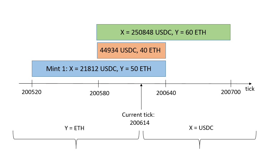
Panel B: Liquidity by tick range

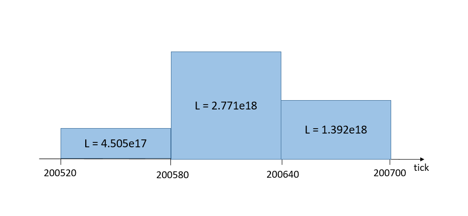
Appendix E

Files/variables.tex

Internet Appendix

Table IA1: Repositioning intensity and liquidity concentration: Large LPs. This table replicates our analysis from Table 5 for a subset of large LPs. For each pool and chain, we sum up total minted and burned liquidity (in $) for each individual LP over our entire sample period. We then define large LPs as those in the top quartile of our sample distribution. Panel A reports results for the low-fee pool (ETH/USDC 0.05%), and Panel B for the high-fee pool (ETH/USDC 0.3%). $Arbitrum$ ($Polygon$) takes value of 1 for Arbitrum (Polygon) pools, and zero for Ethereum pools. Model (1) reports the results for the first-stage regression, with repositioning intensity of LPs, $Intensity$, as the dependent variable and $Arbitrum$ as the main explanatory variable, which is used as an instrument for the endogenous $Intensity$. Model (2) reports results for the second-stage regression, with liquidity concentration within 2% of the market price, $Conc$, as the dependent variable. The set of instruments consists of all explanatory variables, except that $Intensity$ is replaced with $Arbitrum$. The table shows corresponding results for Polygon pools in Models (3) and (4), with $Polygon$ used as an instrument for the endogenous $Intensity$. Models (5) and (6) use $BlockScaling$ that takes value of 1 for both Arbitrum and Polygon pools, and zero for Ethereum pools, as an instrument. The vector of control variables consists of $Volume$, $Volatility$ and $|Return|$. See Appendix E for a detailed description of variable definitions. All regressions include hour- and day-fixed effects, with standard errors clustered at the day level. T-statistics of the two-tailed t-test with the null-hypothesis of a coefficient equaling zero are reported in parentheses. ***, **, and * indicate statistical significance at the 1%, 5%, and 10% level, respectively.

Panel A: ETH/USDC 0.05%
	Arbitrum				Polygon				BlockScaling
	Int		Conc		Int		Conc		Int		Conc
			2%				2%				2%
	(1)		(2)		(3)		(4)		(5)		(6)
$Arbitrum$	0.25	***
	(32.87)
$Polygon$					0.19	***
					(27.33)
$BlockScaling$									0.21	***
									(35.16)
$Intensity$			0.08	***			0.10	***			0.10	***
			(44.84)				(49.92)				(52.41)
$Volume$	-0.01		0.01	***	-0.01	***	0.01	***	0.01	**	0.01	***
	(-1.58)		(46.49)		(-3.70)		(50.86)		(2.15)		(53.91)
$Volatility$	-0.53		-1.56	***	0.18		-1.48	***	-1.53	***	-1.37	***
	(-0.91)		(-39.64)		(0.38)		(-41.87)		(-3.17)		(-47.51)
$|Return|$	22.56	***	-2.51	***	17.12	***	-2.26	***	21.25	***	-2.80	***
	(16.61)		(-24.52)		(16.72)		(-26.56)		(19.10)		(-34.40)
$Observations$	90,401		90,401		119,075		119,075		181,095		181,095
$HourFE$	Yes		Yes		Yes		Yes		Yes		Yes
$DateFE$	Yes		Yes		Yes		Yes		Yes		Yes

Panel B: ETH/USDC 0.3%
	Arbitrum				Polygon				BlockScaling
	Int		Conc		Int		Conc		Int		Conc
			2%				2%				2%
	(1)		(2)		(3)		(4)		(5)		(6)
$Arbitrum$	0.17	***
	(14.44)
$Polygon$					0.21	***
					(28.36)
$BlockScaling$									0.18	***
									(25.46)
$Intensity$			0.06	***			0.17	***			0.11	***
			(27.21)				(40.20)				(41.73)
$Volume$	-0.19	***	0.06	***	-0.02		0.04	***	-0.02		0.07	***
	(-4.74)		(37.89)		(-1.10)		(18.73)		(-1.07)		(48.48)
$Volatility$	3.27	***	-1.13	***	-0.05		-0.95	***	0.22		-1.47	***
	(4.64)		(-33.73)		(-0.10)		(-14.01)		(0.41)		(-33.85)
$|Return|$	9.76	***	-0.76	***	18.27	***	-3.23	***	18.37	***	-2.15	***
	(7.63)		(-9.61)		(11.36)		(-16.39)		(12.84)		(-17.85)
$Observations$	34,264		34,264		38,424		38,424		54,151		54,151
$HourFE$	Yes		Yes		Yes		Yes		Yes		Yes
$DateFE$	Yes		Yes		Yes		Yes		Yes		Yes

Table IA2: Repositioning precision and liquidity concentration: Arbitrum and Polygon. This table presents results of instrumental variable regressions that test causal effect of repositioning precision of LPs, separately for Arbitrum and Polygon. We use three measures of repositioning precision: $Gap$, $Length$ and $Precision$. See Appendix E for a detailed description of variable definitions. Panel A reports results for the low-fee pool (ETH/USDC 0.05%), and Panel B for the high-fee pool (ETH/USDC 0.3%). Model (1)-(3) report the results of the second-stage regressions with liquidity concentration within 2% as the dependent variable. $Arbitrum$ is used as an instrument for the endogenous repositioning precision. Models (4)-(6) present corresponding results, with $Polygon$ used as an instrument for repositioning precision. The vector of control variables consists of $Volume$, $Volatility$ and $|Return|$. All regressions include hour- and day-fixed effects, with standard errors clustered at the day level. T-statistics of the two-tailed t-test with the null-hypothesis of a coefficient equaling zero are reported in parentheses. ***, **, and * indicate statistical significance at the 1%, 5%, and 10% level, respectively.

Panel A: ETH/USDC 0.05%
	Arbitrum						Polygon
	Conc, $2\%$						Conc, $2\%$
	(1)		(2)		(3)		(4)		(5)		(6)
$Gap$	-2.73	***					-4.76	***
	(-17.52)						(-12.54)
$Length$			-0.35	***					-0.50	***
			(-28.48)						(-24.57)
$Precision$					0.12	***					0.22	***
					(24.31)						(18.00)
$Volume$	0.01	***	0.01	***	0.01	***	0.01	***	0.01	***	0.01	***
	(15.97)		(35.36)		(25.24)		(8.27)		(18.51)		(16.40)
$Volatility$	-1.15	***	-1.41	***	-1.28	***	-0.65	***	-1.07	***	-0.89	***
	(-11.91)		(-22.52)		(-19.44)		(-4.53)		(-14.87)		(-10.39)
$|Return|$	-1.64	***	-2.37	***	-1.15	***	-2.12	***	-2.75	***	-1.76	***
	(-11.24)		(-16.20)		(-11.20)		(-8.86)		(-16.42)		(-11.02)
$Observations$	47,987		47,987		47,987		65,146		65,146		65,146
$HourFE$	Yes		Yes		Yes		Yes		Yes		Yes
$DateFE$	Yes		Yes		Yes		Yes		Yes		Yes

Panel B: ETH/USDC 0.3%
	Arbitrum						Polygon
	Conc, $2\%$						Conc, $2\%$
	(1)		(2)		(3)		(4)		(5)		(6)
$Gap$	-0.77	***					-8.76	***
	(-7.29)						(-3.71)
$Length$			-0.06	***					-0.30	***
			(-9.89)						(-16.98)
$Precision$					0.07	***					0.24	***
					(8.06)						(15.80)
$Volume$	0.04	***	0.05	***	0.04	***	-0.07		0.02	***	-0.00
	(9.37)		(17.81)		(10.15)		(-1.60)		(4.26)		(-0.13)
$Volatility$	-0.81	***	-0.97	***	-0.59	***	1.79		-0.61	***	0.24
	(-8.89)		(-15.25)		(-6.23)		(1.52)		(-4.41)		(1.29)
$|Return|$	-0.45	***	-0.27	***	-0.31	***	-2.19	**	-1.35	***	-2.26	***
	(-3.91)		(-3.65)		(-3.01)		(-2.00)		(-6.66)		(-7.58)
$Observations$	7,153		7,153		7,153		10,746		10,746		10,746
$HourFE$	Yes		Yes		Yes		Yes		Yes		Yes
$DateFE$	Yes		Yes		Yes		Yes		Yes		Yes

References

- [1] Hayden Adams et al. “Uniswap v3 whitepaper” In Tech. rep., Uniswap, https://uniswap.org/whitepaper-v3.pdf, 2021
- [2] Jun Aoyagi “Liquidity provision by automated market makers” In Working paper, Hong Kong University of Science and Technology, 2020
- [3] Jun Aoyagi and Yuki Ito “Coexisting Exchange Platforms: Limit Order Books and Automated Market Makers” In Working paper, Hong Kong University of Science and Technology, 2021
- [4] Angelo Aspris, Sean Foley, Jiri Svec and Leqi Wang “Decentralized exchanges: The “wild west” of cryptocurrency trading” In International Review of Financial Analysis 77, 2021, pp. 101845
- [5] Andrea Barbon and Angelo Ranaldo “On The Quality Of Cryptocurrency Markets: Centralized Versus Decentralized Exchanges” In Working paper, University of St. Gallen, 2021
- [6] Agostino Capponi and Ruizhe Jia “The Adoption of Blockchain-based Decentralized Exchanges” In Working paper, Columbia University, 2021
- [7] Álvaro Cartea, Fayçal Drissi and Marcello Monga “Decentralised finance and automated market making: Predictable loss and optimal liquidity provision” In Working paper, Oxford-Man Institute of Quantitative Finance, 2023
- [8] Nir Chemaya and Dingyue Liu “Estimating Investor Preferences for Blockchain Security” In Working paper, University of California, Santa Barbara, 2022
- [9] Sean Foley, Peter O’Neill and Tālis J. Putniņš “A better market design? Applying ’Automated Market Makers’ to Traditional Finance Markets” In Working paper, University of New South Wales, 2023
- [10] Joel Hasbrouck, Thomas J Rivera and Fahad Saleh “The need for fees at a DEX: How increases in fees can increase DEX trading volume” In Working paper, Wake Forest University, 2022
- [11] Joel Hasbrouck, Thomas J Rivera and Fahad Saleh “An economic model of a decentralized exchange with concentrated liquidity” In Working paper, Wake Forest University, 2023
- [12] Lioba Heimbach, Eric Schertenleib and Roger Wattenhofer “Risks and Returns of Uniswap V3 Liquidity Providers” In Working paper, ETH Zürich, 2022
- [13] Terrence Hendershott, Charles M Jones and Albert J Menkveld “Does algorithmic trading improve liquidity?” In Journal of Finance 66.1 Wiley Online Library, 2011, pp. 1–33
- [14] Albert S Kyle “Continuous auctions and insider trading” In Econometrica 53 JSTOR, 1985, pp. 1315–1335
- [15] Alfred Lehar and Christine A Parlour “Decentralized Exchange: The Uniswap Automated Market Maker” In Journal of Finance, forthcoming, 2021
- [16] Alfred Lehar, Christine A Parlour and Marius Zoican “Liquidity Fragmentation on Decentralized Exchanges” In Working paper, Haas School of Business, UC Berkeley, 2022
- [17] Andreas Park “The Conceptual Flaws of Decentralized Automated Market Making” In Management Science 69.11, 2023, pp. 6731–6751