Exploration and Exploitation of Unlabeled Data for Open-Set Semi-Supervised Learning

Abstract

In this paper, we address a complex but practical scenario in semi-supervised learning (SSL) named open-set SSL, where unlabeled data contain both in-distribution (ID) and out-of-distribution (OOD) samples. Unlike previous methods that only consider ID samples to be useful and aim to filter out OOD ones completely during training, we argue that the exploration and exploitation of both ID and OOD samples can benefit SSL. To support our claim, i) we propose a prototype-based clustering and identification algorithm that explores the inherent similarity and difference among samples at feature level and effectively cluster them around several predefined ID and OOD prototypes, thereby enhancing feature learning and facilitating ID/OOD identification; ii) we propose an importance-based sampling method that exploits the difference in importance of each ID and OOD sample to SSL, thereby reducing the sampling bias and improving the training. Our proposed method achieves state-of-the-art in several challenging benchmarks, and improves upon existing SSL methods even when ID samples are totally absent in unlabeled data.

1 Introduction

Semi-supervised learning (SSL) is a promising machine learning approach that exploits unlabeled data to mitigate the costly data labeling process. Given a small set of labeled data and a large set of unlabeled data, SSL aims to train a classifier that surpasses its supervised variant trained only on the labeled dataset. Classic SSL techniques include consistency regularization [1, 2], pseudo labeling (a.k.a. self-training) [3, 4] and entropy minimization [5]. Recently, FixMatch [6] achieved state-of-the-art performance by simply combining consistency regularization with pseudo labeling. Although being effective, traditional SSL methods implicitly assumed that the unlabeled data share the same label space with the labeled data during training, which limits their application in the open-set real-world scenarios.

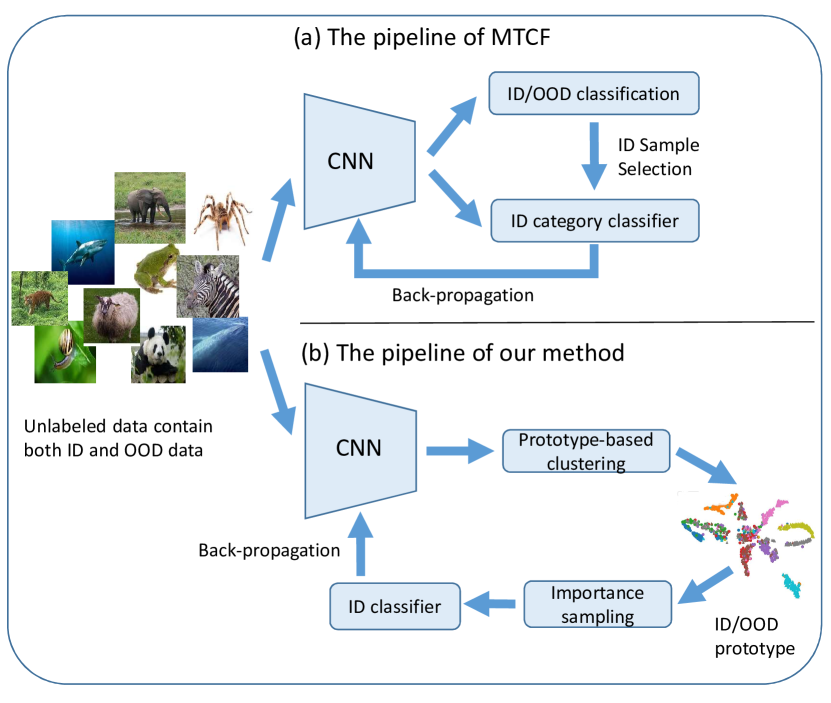
Figure 1: The comparison between our method and MTCF[7]. MTCF sets an independent OOD detection branch to the backbone, and performs ID/OOD classification on the features. OOD samples are excluded from semi-supervised learning. Different from MTCF, our method first clusters both ID and OOD features to prototypes. Prototypes are assigned ID/OOD labels and unlabeled samples are sampled by their importance and prototypes. Our method exploits both ID and OOD data for the backbone training.

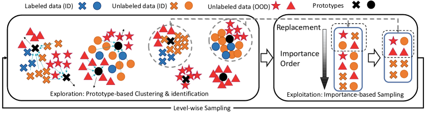
Figure 2: Exploration and exploitation of the unlabeled data including in-distribution (ID) and out-of-distribution (OOD) samples. Exploration: we cluster ID and OOD samples in each mini-batch and identify them accordingly based on an exploration of the inherent similarity and difference of their features (represented by prototypes). Exploitation: we exploit the different importance of each ID and OOD sample in SSL to reduce the sampling bias during training.

Open-set SSL extends SSL to open-set datasets where the unlabeled data contain both in-distribution (ID) and out-of-distribution (OOD) samples. Specifically, ID samples share the same label space with labeled data while OOD samples may be out of that label space. Yu et al.[7] pioneered this direction and proposed to eliminate the negative effects of OOD samples using an OOD detector [8]. Thanks to the OOD detector, they identified high-confidence ID samples and gradually incorporated them into the training of a MixMatch [9] model with their multi-task curriculum framework.

Although MTCF [7] is effective, we argue that it has the following two shortcomings. First, it overlooks the role of OOD samples in feature learning. In their method, OOD samples are excluded from SSL whereas we argue that if being properly used, OOD samples can benefit feature learning and thus SSL, especially when there are few ID samples in the unlabelled dataset. Second, their method depends on the performance of its OOD detector and thus performs poorly on high-variance datasets where the ambiguity between ID and OOD samples makes it prone to misclassification. As pointed out by previous studies[10], near-OOD tasks where OOD samples are close to ID ones can greatly lower the performance of OOD detection method. Simply filtering out all OOD samples can be difficult and thus degrades the performance of semi-supervised training when OOD samples dominate the unlabeled dataset. In addition, their evaluation is based on synthetic OOD samples (e.g. Gaussian noise, Uniform noise) and images of completely irrelevant topics, which may not generalize to real-world scenarios where OOD samples can be “close” to ID ones.

In previous semi-supervised studies, pseudo labeling is an important technique that can utilize the unlabeled data and thus improve the performance of semi-supervised methods. Pseudo labeling encourages the model to output high-confidence prediction for unlabeled samples and thus construct a better feature extractor[6]. However, if unlabeled data contains both ID and OOD images, pseudo-labeling-based methods will force ID and OOD samples with the same label prediction to get closer, which degrades the performance of the feature extractor and the accuracy of ID/OOD classification. Therefore, our method aims to construct and preserve the inner structure of both ID and OOD features to train a better feature extractor and to facilitate the ID/OOD classification.

In this paper, we address the aforementioned shortcomings of open-set SSL by exploring and exploiting the unlabeled data including both ID and OOD samples (Fig. 2). Specifically, we first propose a prototype-based clustering and identification algorithm that clarifies the ambiguity between ID and OOD samples by exploring the inherent similarity and difference among their features, and thus better identifies the unlabeled samples. Then, we propose a novel importance sampling method that reduces the sampling bias by exploiting the difference in importance of each ID and OOD sample to SSL, thereby improving training. We implement this method with our newly proposed cascading pooling strategy, which increases the density of ID samples in mini-batches and further stabilizes training. Empirically, we verify the effectiveness of our method on three standard benchmark datasets (CIFAR-100 [11], SVHN [12] and TinyImageNet [13]) and a new dataset, DomainNet-Real [14], which is more challenging and realistic. In summary, our contributions include:

• We demonstrate that the performance of open-set semi-supervised learning (SSL) can be improved by utilizing out-of-distribution (OOD) samples.

• We design a novel prototype-based clustering and identification algorithm and demonstrate its effectiveness in feature learning.

• We propose a new importance-based sampling method that reduces sampling bias and improves training.

• We introduce a new benchmark that is more challenging and closer to real-world scenarios. Extensive experimental results on three standard benchmark datasets as well as our introduced benchmark demonstrate the superiority of our proposed method.

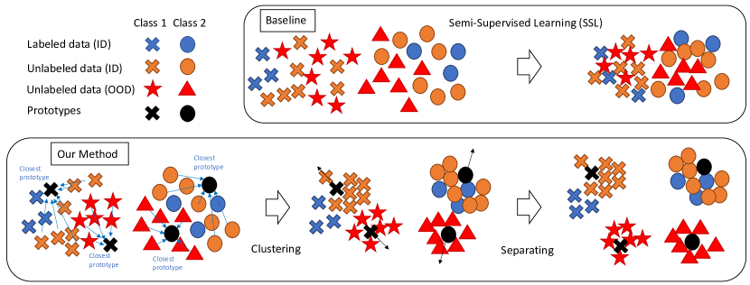
Figure 3: Illustration of our prototype-based clustering method. Top row: Semi-supervised learning (SSL) methods might be confused by the OOD samples and incorrectly assign in-distribution (ID) pseudo labels to them, which degrades their performance. Bottom row: With our clustering method, ID and OOD samples are pushed away from each other towards a set of pre-defined prototypes (black marks), which clarifies the ambiguity between ID and OOD samples and facilitates ID/OOD identification. The positions of the prototypes are dynamically updated during training.

2 Related Works

Semi-Supervised Learning (SSL) addresses the scarcity of labeled data by leveraging the relationship between a small amount of labeled data and a large amount of unlabeled data. In general, two common SSL techniques that are widely applied to semi-supervised learning are consistency regularization and pseudo labeling (a.k.a. self-training). Consistency regularization (CR) [2, 15, 1, 16] assumes that the classification results should only rely on the semantics of input images, and penalizes the change of model outputs against the perturbation or augmentation of input images. Some CR methods employ adversarial perturbation or dropout [17, 18] on the input images while data augmentation [19, 1] is widely recognized to be more effective. From another perspective, pseudo labeling [3, 4] assigns pseudo labels to unlabeled data according to the model’s prediction confidence and steers its own training with those pseudo labels. FixMatch[6] combines the ideas of pseudo labeling and consistency regularization, and achieves state-of-the-art performance on several benchmarks for semi-supervised learning. FixMatch utilizes two different augmentations of the input image, strong augmentation, and weak augmentation, and trains the model with the strong-augmented images and the pseudo labels generated by corresponding weak-augmented images. Similar to pseudo labeling, Entropy minimization [5] encourages the model to output low-entropy (i.e. high confidence) prediction for unlabeled samples. Besides, there have been other techniques for semi-supervised learning. Temporal ensemble[2] forms a consensus prediction for the unlabeled data using the outputs of the network-in-training on different epochs. Mean teacher[20] averages model weights instead of label predictions to avoid the problem that temporal ensemble becomes unwieldy when learning from large datasets. FlexMatch[21] proposes a curriculum learning approach for semi-supervised learning to leverage unlabeled data according to the model’s learning status. Some self-supervised methods[22] also employ prototype-based methods for semi-supervised learning, however, their clustering strategies are purely unsupervised and not applicable to OOD detection during training.

Out-Of-Distribution (OOD) Identification [8, 23, 24, 25, 26] aims to identify the OOD samples in a given dataset which consists of both In-Distribution classes and Out-Of-Distribution samples. For image classification, conventional methods like density estimation or nearest neighbor [27, 28, 29] are not applicable due to the high dimensionality of image feature space. Addressing this issue, DNN-based OOD detectors [8, 30] have been proposed. Based on the observation that ID samples tend to have higher softmax scores, Hendrycks et al. [30] propose a baseline method for OOD detection without retraining networks. Liang et al. [8] improve such a baseline by introducing temperature scaling in the softmax function to increase the softmax score gap between ID and OOD samples. The difficulty of the OOD detection depends on how semantically close to the inlier classes, i.e., ID classes are to the outliers, i.e., OOD samples. Winkens et al. [10] distinguish the difficulty difference between near-OOD tasks and far-OOD tasks by the difference of state-of-the-art performance for area under the receiver operating characteristic curve (AUROC). Some methods[31, 32, 33, 34] tackle the OOD detection problem by class conditional Gaussian distributions, energy function or rectified activations. However, most of them detect the OOD samples post hoc, which is not suitable for open-set semi-supervised learning.

Open-Set Semi-Supervised Learning aims to develop robust SSL algorithms which work on “dirty” unlabeled data that contain OOD samples. Oliver et al. [35] first pointed out that the performance of SSL techniques can degrade drastically when the unlabeled data contain a different distribution of classes. This inspires MTCF [7] which incorporates an OOD detection branch to MixMatch [9] and works by gradually adding high-confidence ID samples to semi-supervised training. However, it ignores the contribution of consistency regularization to SSL, which is independent to OOD detection. From this perspective, OOD samples are harmless and can even be beneficial. Thus, excluding them from training may not be the optimal solution and can be impractical for big datasets containing a large proportion of OOD samples. To this end, we propose to utilize OOD samples instead of filtering them out during training. As a concurrent work, Luo et al. [36] viewed the categorical difference between OOD and ID samples as a distributional difference and attempted to reduce the distribution divergence using style transfer. They also explored the OOD samples during training via unsupervised data augmentation [37]. UASD [38] tackled a problem called Class Distribution MisMatch where some classes in the labeled data are absent in the unlabeled data, and vice versa. Although looks similar, this problem is different from ours. Huang et al. [39] propose a cross-modal matching strategy to detect OOD samples and train the network to match samples to an assigned one-hot class label.

3 Preliminary

Given a small labeled dataset $\mathcal{X}=\{(x_{i},y_{i})\}_{i=1}^{N_{l}}$ and a large unlabeled dataset $\hat{\mathcal{X}}=\{\hat{x}_{i}\}_{i=1}^{N}$ where $N\gg N_{l}$ and $y_{i}\in(1,...S)$, semi-supervised learning for classification aims to learn a model that performs best by utilizing both $\mathcal{X}$ and $\hat{\mathcal{X}}$. Different from traditional semi-supervised learning, open-set semi-supervised learning aims to utilize an unlabeled dataset $\hat{\mathcal{X}}$ containing out-of-distribution samples whose ground truth labels are not in $(1,...S)$. Our method aims to train a model to achieve higher accuracy on the test set which contains only in-distribution data.

4 Method

Our method has two components: i) a prototype-based clustering and identification algorithm that learns better representations for the identification of In-Distribution (ID) and Out-Of-Distribution (OOD) samples by clustering them in an unsupervised way; ii) an importance sampling method that samples unlabeled data according to their importance to SSL, thereby reducing the sampling bias and improving the training (Fig. 4). Specifically, our clustering and identification algorithm helps pseudo-labeling by pushing ambiguous ID and OOD samples away from each other (towards different prototypes) in the feature space. Note that as an unsupervised representation learning method, our clustering process benefits a lot from the OOD data that “augment” the dataset. The resulting clusters can be binarily identified as ID and OOD ones according to labeled data. Based on the identification, we design a novel importance sampling method that assigns importance scores to unlabeled data and samples them accordingly. This addresses the problem of random sampling where early-identified ID samples are over-sampled while later ones are under-sampled. Furthermore, we devise a cascading pooling strategy to improve the density of ID samples in mini-batch training, which further stabilizes the training. The overview of our method is shown in Algorithm 1.

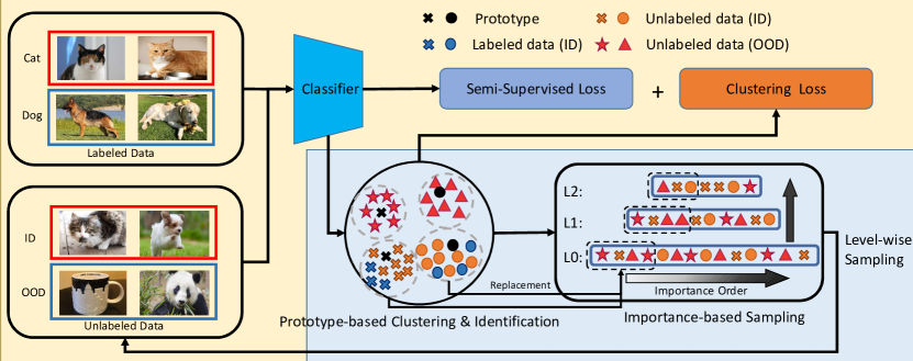
Figure 4: Overview of our method. We propose two techniques, a prototype-based clustering and identification algorithm, and an importance-based sampling method to improve the performance of open-set semi-supervised learning (SSL). Our clustering and identification algorithm clusters samples at the feature level and thus facilitates feature learning by increasing the distances between ID and OOD samples. Our importance-based sampling method facilitates SSL by reducing the sampling bias during training.

Algorithm 1 Overview of our method.

0:  initialized prototypes

0:  clustering loss $L_{c}$, semi-supervised loss $L_{SSL}$

1:  for number of training iterations do

2:     Sample a minibatch of labeled samples

3:     Sample a minibatch of unlabeled samples from our pyramid of sample pools

4:     Compute semi-supervised learning loss $L_{SSL}$ for labeled and unlabeled minibatches

5:     for each sample do

6:        for each $s\in\{1,2,...,S\}$ do

7:           Compute $L_{c}$ (Eq. 2) using our prototype-based clustering algorithm

8:           Update the prototypes using Eq. 5

9:           Update the sample pools accordingly

10:        end for

11:     end for

12:  end for

4.1 Prototype-based Clustering and Identification

As Fig. 3 (top row) shows, ID and OOD samples are mixed in unlabeled data. Thus, a key defect of open-set pseudo labeling is that OOD samples can easily be misclassified as ID samples, thereby confusing the feature extractor. Addressing this issue, we propose a prototype-based clustering algorithm to clarify the ambiguity between ID and OOD samples (Fig. 3, bottom row). Let $F$ be an SSL classifier, $\hat{x}_{i}$ be a sample in the unlabeled dataset $\hat{\mathcal{X}}=\{\hat{x}_{i}\}_{i=1}^{N}$, $\hat{s}$ be the pseudo label of $\hat{x}_{i}$ assigned by $F$, $F(\hat{x}_{i})$ be the output probabilities of $F$ with input $\hat{x}_{i}$, and $f(\hat{x}_{i})$ be the normalized feature extracted by $f$ (a subnetwork of $F$, a.k.a. a feature extractor), our clustering algorithm is detailed as follows:

Prototype Initialization. This step aims to set up $K$ initial prototypes $p^{s}_{j},j\in\{1,2,...,K\}$ for each class $s\in\{1,2,...,S\}$. First, we pretrain $F$ until each class $s$ contains at least $M$ unlabelled samples, $M\ll N/S$ where $N$ is the unlabeled set size. These samples are assigned pseudo labels $\hat{s}$. Then, for each class $s$, we extract the features of all its unlabeled samples by $f$ and initialize our prototypes $p_{j}^{s}$ (Fig. 3, black marks) as the $k$-means cluster centers of the extracted features. In this step, both $K$ and $M$ are hyperparameters.

Clustering Loss. For each unlabeled sample $\hat{x}_{i}$ in a mini-batch during training, given its pseudo label $\hat{s}$ (generated by SSL method) and the associated $K$ prototypes $p^{s}_{j},j\in\{1,2,...,K\}$ of class $s$, we define our prototype-based clustering loss as:

$$L^{s}_{c}(\hat{x}_{i}) =$$ (1)

$$- \log{\frac{\mathrm{exp}(f(\hat{x}_{i})\cdot p_{*}^{s}/\tau)}{\sum^{K}_{j=1}{\mathrm{exp}(f(\hat{x}_{i})\cdot p_{j}^{s}/\tau)}}\mathbbm{1}(\max(F(\hat{x}_{i}))>t_{c})},$$

where $\mathbbm{1}$ is an indicator function, $t_{c}$ is a threshold parameter, $p_{*}^{s}$ is the prototype that is closest to $f(\hat{x}_{i})$ in Euclidean space, $\tau$ is a temperature parameter used in self-supervised learning [40]. Intuitively, minimizing $L^{s}_{c}(\hat{x}_{i})$ guides classifier $F$ to generate features $f(\hat{x}_{i})$ closer to $p^{s}_{*}$ but further to other prototypes. Thus, the overall loss across a mini-batch of unlabeled samples is:

$$L_{c}=\sum_{j=1}^{BS}L^{s}_{c}(\hat{x}_{j})$$ (2)

where $BS$ is the batch size. $L_{c}$ is used as an additional loss term in the SSL loss function.

In addition to the clustering loss for unlabeled data, we further apply a similar loss to the labeled data, clustering them to the same centers. Specifically, given a labeled sample $x_{i}$ ($1\leq i\leq N_{y}$) and its ground truth label $y$, where $N_{y}$ is the total number of labeled samples with label $y$, we define the loss as:

$$L_{labeled}^{y}(x_{i})=-f(x_{i})\cdot q_{y}+L_{c}^{s}(x_{i}),$$ (3)

where $q_{y}$ is the normalized feature center of class $y$:

$$q_{y}=\mathrm{normalize}(\sum_{i=1}^{N_{y}}f(x_{i})).$$ (4)

In Eq. 3, the first term aims to cluster all labeled samples of the same class towards their normalized feature center $q_{y}$, preventing them from being misaligned to different ID/OOD centers; the second term applies the same clustering loss for unlabeled data (Eq. 1) to labeled data, indicating that both the labeled and unlabeled ID samples should be clustered to the same centers. The clustering loss clusters the features of both labeled and unlabeled data in a semi-supervised manner, thus separates the ID and OOD data into different cluster centers.

Prototype Update. At the same time, for each sample $\hat{x}_{i}$ in a mini-batch during training, we dynamically update its nearest prototype $p^{s}_{*}$ as a moving average:

$$p_{*,(t+1)}^{s}=\alpha p_{*,(t)}^{s}+\beta f(\hat{x}_{i}),$$ (5)

where $\alpha=0.99$ and $\beta=0.01$ are weighting parameters following the common practice of momentum update.

With our prototype-based clustering algorithm, pseudo-labeled samples in each class $s$ are clustered according to the similarity of their features. As a result, heterogeneous samples are pushed away from each other. This helps SSL as the difference between OOD and ID samples are also clarified, thereby helping the feature extractor to learn better representations. Thus, OOD samples are less likely to be misclassified as ID samples and damage the self-training. Based on the clustering results, we identify ID/OOD samples as follows.

Sample Identification. First, we identify the unlabeled ID samples to be included in the pools according to their distances to the labelled ID samples in the labeled dataset $\mathcal{X}=\{(x_{i},s_{i})\}_{i=1}^{N_{l}}$, $s_{i}\in\{1,2,...,S\}$ where $S$ is the number of classes. Let $f(x_{i})$ be the normalized feature of $x_{i}$ that is extracted by $f$, we can calculate the per-class feature centers of the labeled data as:

$$O_{s}=\frac{\sum_{i=1}^{N_{l}}\mathbbm{1}(s_{i}=s)f(x_{i})}{\sum_{i=1}^{N_{l}}\mathbbm{1}(s_{i}=s)},s\in\{1,2,...,S\}$$ (6)

where $\mathbbm{1}$ is an indicator function. Since all labeled data are ID, an unlabeled sample with pseudo label $s$ tend to be ID if its corresponding prototype $p_{*}^{s}$ is close to $O_{s}$. Therefore, for each class $s$, we compute the Euclidean distances from $O_{s}$ to each of its prototypes $p^{s}_{j}$. According to these distances, we sort all prototypes $p^{s}_{j}$ in increasing order and pick the first $N_{id}$ of them as ID prototypes. For each unlabeled sample $\hat{x_{i}}$ in a mini-batch, we identify it as ID if its closest prototype $p_{*}^{s}$ is an ID prototype. Otherwise, $\hat{x_{i}}$ is identified as OOD. In this step, $N_{id}$ is a hyperparameter.

4.2 Importance Sampling for Open-Set SSL

Recalling the definition of Open-set SSL where the dataset contains two types of samples, i.e. ID and OOD samples, it is straightforward to assume that they are of different importance to SSL: ID samples are useful while OOD ones are less relevant for the target task. Such an assumption motivates the selection of ID samples in SSL that is widely employed in previous methods. Despite that OOD samples can help the training of semi-supervised methods, overwhelming OOD samples in mini-batches will unstabilize the training and lower the performance when the images are large and the batch size is small. Therefore, We follow the ID sample selection paradigm and try to improve the performance by making the classifier concentrate on ID samples while utilizing the information of OOD samples. Unlike previous methods, we noticed that ID samples are dynamically identified during training. Thus, the ID samples identified earlier occurs more often in random sampling and are thus biased. This is undesirable as they can soon be well-learnt and contribute less to the training than newly identified ones. To this end, we propose a novel importance sampling method for mini-batch sampling during training that assigns importance scores to unlabeled samples and only maintains the important ones in the sample pools as follows.

Importance-based Sample Pools. After identification, the identified OOD samples are assigned importance scores of 0 and excluded from SSL; the identified ID samples are assigned importance scores of $1/I(\hat{x}_{i})$ where $I(\hat{x}_{i})$ is the number of times $\hat{x}_{i}$ is identified as an ID sample throughout the training. We maintain the identified ID samples in our per-class importance-based sample pools $P_{s}$, where $s\in\{1,2,...,S\}$ is the class label. We restrict $P_{s}$ to contain at most $N_{p}$ samples, $N_{p}\gg BS$ where $BS$ is the batch size. During mini-batch training, assume that $M$ ID samples are identified for class $s$ in one iteration, we update $P_{s}$ by:

- Case 1. If $P_{s}$ has enough space, we simply add the $M$ ID samples to $P_{s}$.

- Case 2. Otherwise, we compute probability $\mathcal{P}_{\hat{x}_{i}}$ for each sample $\hat{x}_{i}$ in $P_{s}$, $i\in\{1,2,...,N_{P}\}$ using their importance scores as:

$$\mathcal{P}_{\hat{x}_{i}}=\min\{M\frac{I(\hat{x}_{i})}{\sum_{j=1}^{N_{p}}I(\hat{x}_{j})},1\},$$ (7)

Then, we select each sample by probability $\mathcal{P}_{\hat{x}_{i}}$ and obtain $N_{r}$ samples. We replace the first $\min(N_{r},M)$ of them with the newly identified ID samples. Intuitively, an ID sample is more likely to be removed from $P_{s}$ if it is sampled more often, i.e., it is well-learnt.

However, it is difficult to identify ID samples accurately by performing the identification once when the unlabeled set is complicated and OOD data can benefit the semi-supervised training. Besides, the density of ID samples in a mini-batch is important for the performance as we show in Sec 5.3. To this end, we devise a cascading pooling strategy to further improve the density of ID samples as follows, and it can help and stabilize the SSL training by providing high-density ID samples within a mini-batch.

Cascading Sample Pools. Let $S$ be the number of classes, we cascade different sets of sample pools as a pyramid:

• Level 0 of the pyramid is the raw dataset.

• Level 1 is a set of $S$ ID sample pools. The capacity of each sample pool is $N_{P}$.

• Level 2 is a set of $S$ ID sample pools. The capacity of each sample pool is $N_{P}/2$.

• ……

• Level N is a set of $S$ ID sample pools. The capacity of each sample pool is $N_{P}/2^{N-1}$.

During training, we circularly draw mini-batches of samples in a level-wise manner from Level 0 to Level N. In each training iteration, we draw samples evenly from the $S$ sample pools in the same level and apply ID sample identification to it. The newly identified ID samples are used to update the sample pools at the next level.

5 Experiment

5.1 Experimental Setup

Datasets. Following the common practice in SSL evaluation [6], we test our method on four benchmark datasets:

- CIFAR-100 [11]: a dataset consisting of 100 classes of natural images. Each class contains 500 training images and 100 testing images.

- SVHN [12]: a dataset consisting of 10 classes of digits images. It contains 73,257 and 26,032 digits images for training and testing respectively.

- TinyImageNet: a subset of the ImageNet dataset [13] consisting of 200 classes of natural images. Each class contains 500 training images and 50 test images.

And a more challenging and realistic dataset:

- DomainNet-Real [14]: DomainNet is a dataset consisting of 345 classes of images in 6 domains (e.g. real, painting, sketch). In our experiments, we only use the 172,947 images in its Real domain as we observed that FixMatch [6] performs poorly in some domains.

TABLE I: Experimental results on Open-Set Semi-Supervised Learning. Our method outperforms MTCF [7] and improves FixMatch [6] by a significant margin. ID / OOD: the number of classes whose images are defined as ID and OOD samples respectively. $(\cdot)$ / 50k^∗: to balance the numbers of ID and OOD samples, we sample 50k images from the classes other than $(\cdot)$ in DomainNet-Real as OOD samples. ^†: DS³L consumes too much memory and time on DomainNet-Real and cannot run on commodity workstations.

Datasets	DomainNet-Real		CIFAR-100		TinyImageNet
ID / OOD	10 / 50k∗	20 / 50k∗	10 / 90	20 / 80	10 / 190	20 / 180
Labeled Only	48.5$\pm$1.0	41.6$\pm$0.7	47.3$\pm$1.8	40.0$\pm$0.4	36.9$\pm$2.3	32.2$\pm$0.9
FixMatch [6]	52.8$\pm$2.9	49.7$\pm$2.5	80.8$\pm$0.9	72.2$\pm$0.2	68.9$\pm$0.7	53.6$\pm$1.0
MTCF [7]	54.2$\pm$1.8	46.3$\pm$0.4	59.8$\pm$0.6	46.2$\pm$1.0	52.4$\pm$1.2	46.5$\pm$0.6
DS3L[41]†	–	–	57.0$\pm$0.7	40.2$\pm$1.0	52.2$\pm$2.7	40.0$\pm$1.6
Energy[32]	50.1$\pm$1.8	45.9$\pm$1.0	82.5$\pm$0.7	72.9$\pm$1.6	67.3$\pm$2.0	56.5$\pm$1.5
ReAct[34]	50.1$\pm$1.1	46.6$\pm$0.7	82.9$\pm$0.7	73.3$\pm$2.0	69.5$\pm$1.7	57.7$\pm$2.0
OpenMatch[42]	54.8$\pm$2.6	50.4$\pm$1.2	83.0$\pm$1.0	73.3$\pm$2.5	68.7$\pm$2.8	54.8$\pm$1.0
Ours	59.4$\pm$0.3	54.3$\pm$1.2	85.5$\pm$0.8	76.0$\pm$1.1	71.4$\pm$0.7	58.5$\pm$1.1
Clean	63.5$\pm$0.7	60.7$\pm$0.8	84.8$\pm$0.7	72.3$\pm$0.4	79.5$\pm$0.8	60.3$\pm$0.3

Implementation Details. We implement our method on top of FixMatch [6], a state-of-the-art SSL algorithm. In addition to the relatively standard pseudo labeling, FixMatch used another common SSL technique: consistency regularization. In a nutshell, it encourages the SSL classifier to output the same value for two variants of an unlabeled sample $\hat{x}_{i}$: a weak-augmented variant $\hat{x}^{a}_{i}$ and a strong-augmented variant $\hat{x}^{b}_{i}$. Accordingly, for class $s$ and sample $\hat{x}_{i}$, we extend $L^{s}_{c}$ (Eq. 1) to $L_{c}^{s,\mathrm{CR}}$ as follows:

$$L_{c}^{s,\mathrm{CR}}(\hat{x}_{i})=L^{s}_{c}(\hat{x}^{a}_{i})+L^{s}_{c}(\hat{x}^{b}_{i})$$ (8)

Note that we use the same target prototype $p_{*}^{s}$ that is closest to the weak-augmented variant $\hat{x}^{a}_{i}$ for both $L^{s}_{c}(\hat{x}^{a}_{i})$ and $L^{s}_{c}(\hat{x}^{b}_{i})$ because i) heuristically, $\hat{x}^{a}_{i}$ is weak-augmented and thus closer to $\hat{x}_{i}$ in the feature space; ii) in line with consistency regularization, $\hat{x}^{a}_{i}$ and $\hat{x}^{b}_{i}$ share the same semantic meanings and should be in the same cluster, i.e. with the same prototype. Similarly, we only use the weak-augmented variants of unlabeled samples in prototype update and sample identification. Following FixMatch, we employ different network architectures for different datasets. We tune the hyper-parameters using a small validation set.

• For CIFAR-100, SVHN and TinyImageNet, we follow FixMatch [6] and use the same architecture based on Wide ResNet (WRN 28$\times$8) [43]. All images are resized to 32 $\times$ 32. We set the number of prototypes $K=10$ and the weight of $L_{c}$ as 0.01 when added to the FixMatch loss function. Following [40], we set $\tau=0.07$ and $t_{c}=0.98$, which is slightly higher than FixMatch’s pseudo labeling threshold of 0.95. We use the same hyperparameters of FixMatch [6] in the semi-supervised learning (SSL) part of our method. We run our method on 1 Nvidia Tesla V100 GPU with 16GB memory and set the batch size as 64 for labeled data and 448 (64$\times$7) for unlabeled data. We report the experimental results after 100 epochs of training.

• For DomainNet-Real, we use the ResNet-50 [44] architecture. All images are resized to 224$\times$224. We set the number of prototypes $K=30$ and the weight of $L_{c}$ as 0.1 when added to the FixMatch loss function. Following the ImageNet [13] training scheme in FixMatch [6], we set $t_{c}=0.7$ which equals to FixMatch’s pseudo labeling threshold. In our experiment, $N_{id}=K/5$. We use the same hyperparameters of FixMatch [6]. We run our method on 6 Nvidia Tesla V100 GPUs and report the experimental results after 100 epochs of training. For each GPU, we set the batch size as 8 for labeled data and 56 for unlabeled data. Following FixMatch [6], we apply linear warmup to the learning rate for the first 5 epochs of training until it reaches an initial value of 0.4. At epoch 60, we decay the learning rate by multiplying it by 0.1.

Experimental Settings. (1) ID vs. OOD. For CIFAR-100, TinyImageNet and SVHN, ID samples are defined as the images in the first $N$ classes; OOD samples are defined as those in the rest classes. For DomainNet-Real, ID samples are defined as the images in the $N$ classes with the most images; OOD samples are defined as the 50k images sampled from the rest classes, which aims to balance the numbers of ID and OOD samples. (2) Labelled vs. unlabelled. For all datasets, labelled data are defined as the first 25 images and their associated labels in each of the $N$ classes; unlabelled data are defined as the rest images in each of the $N$ classes together with the OOD samples. (3) Training vs. Testing. For DomainNet, for each of the $N$ classes, the testing set is defined as the $100$ images sampled from the unlabelled data in the class; For other three datasets we directly use the pre-defined testing set; the training set is defined as other images (including both labelled and unlabelled data) in the class. Furthermore, we report our method’s average performance of the last 10 epochs over 3 runs using the same random seed set.

TABLE II: Justification of OOD samples’ benefits in SSL. ID / OOD: the number of classes whose images are defined as ID and OOD samples. S10 / C100^∗: 10 ID classes are selected from SVHN and 100 OOD classes are selected from CIFAR-100.

Method	DomainNet-Real
FixMatch [6]	49.7$\pm$2.5
Mask-OOD	54.3$\pm$0.7
SimCLR-OOD	56.7$\pm$0.4
Clean	60.7$\pm$0.8

(a) Normal case

Datasets	CIFAR-100	SVHN	TinyImageNet
ID / OOD	10 / 90	S10 / C100∗	20 / 180
Labeled Only	47.3$\pm$1.8	24.6$\pm$2.4	32.2$\pm$0.9
FixMatch	68.7$\pm$1.5	43.4$\pm$2.7	46.9$\pm$0.4
Ours (Clustering)	73.5$\pm$1.3	50.2$\pm$2.9	52.0$\pm$0.9

(b) Extreme case

5.2 Experimental Result

As Table I shows, our method significantly outperforms previous open-set semi-supervised learning and OOD detection methods including MTCF [7], DS³L[41], Energy[32], ReAct[34] and OpenMatch[42]. To give a better idea on how good our method performs, we provide two additional baselines using FixMatch [6]:

• “Labeled Only”: a FixMatch model trained with labeled data only, which can be viewed as a lower bound.

• “Clean”: a FixMatch model trained with ID samples only, which can be viewed as an improved baseline.

We test all methods on three datasets: CIFAR-100, TinyImageNet and DomainNet-Real. As discussed in “Experimental Setup” section, for each dataset, we define the images in its first $N$ ($N=10,20$) classes as the ID samples; the OOD samples are defined accordingly.

• For CIFAR-100 and TinyImageNet, we observed small gaps between FixMatch and Clean, which leaves small room for improvement. Similar to [7], we conjecture that the reason is the relatively simple datasets being used. However, it is interesting to see that our method outperforms “Clean” on CIFAR-100, 10/90 and 20/80 (10/20 ID classes and 90/80 OOD classes from CIFAR-100). This implies that OOD samples are also useful in SSL, which contradicts the common belief that OOD samples are harmful. Nevertheless, we propose to test on a more realistic and challenging dataset: DomainNet-Real.

• For DomainNet-Real, we observed approximately $10\%$ gaps between FixMatch and Clean. In such challenging scenarios, our method also significantly outperforms MTCF [7] and FixMatch [6]. However, there is a considerable gap between our method and “Clean”, which suggests that there is still room for improvement.

In summary, experimental results show that our method performs the best against competing methods in all six settings (two for each dataset), which indicates that the improvement brought by our method can be generalized to a variety of datasets and ID/OOD ratios.

5.3 Do OOD Samples Really Benefit SSL?

This section justifies the motivation of our method: if being “properly” used, OOD samples can benefit SSL. To verify this claim, we assume that all unlabelled samples are perfectly identified as ID and OOD samples before training. Base on this assumption, we propose two strategies to handle the OOD samples when training a FixMatch [6] SSL model:

• Mask-OOD masks all OOD samples by setting their weights to 0 in the FixMatch loss function.

• SimCLR-OOD adds a SimCLR loss term [40] for OOD samples in the FixMatch loss function.

Table II(a) shows the results of Mask-OOD and SimCLR-OOD against the original FixMatch and “Clean” on the DomainNet-Real dataset. We use the same hyperparameters for all methods. Note that Mask-OOD is different from “Clean” as it does not remove the OOD samples and thus keeps the density of ID samples in mini-batches. It can be observed that: i) Mask-OOD works better than the original FixMatch, which is consistent with the common belief that OOD is harmful to SSL. ii) Mask-OOD works worse than SimCLR-OOD, which justifies our claim that compared to filtering out OOD samples, exploiting them properly benefits SSL. iii) Mask-OOD works worse than “Clean”, which indicates that the performance of SSL depends on the density of ID samples in a mini-batch. This motivates the use of our cascading pooling strategy.

Extreme Case Study. To further justify the motivation of our method, we test the performance of our method in an extreme case of open-set SSL where all unlabeled samples are OOD. To implement it, we remove all unlabeled ID samples from the training dataset. Note that we also remove the importance-based sampling method as it is useless in this scenario. Specifically, we compare our method (with clustering only) with FixMatch [6] and its variant “Labeled Only” on three datasets: CIFAR-100, SVHN and TinyImageNet. For CIFAR-100 and TinyImageNet, we set up the labeled ID samples and the unlabelled OOD samples within the same datasets. For SVHN, we set up the labeled ID samples from all its 10 classes and borrow the images from CIFAR-100 as the unlabelled OOD samples. As Table II(b) shows, it can be concluded that Unlabeled OOD samples can still benefit SSL without unlabelled ID samples, which is justified by the observation that both Ours (Clustering) and FixMatch outperform “Labeled Only”. This further justifies our motivation that OOD samples DO benefit SSL.

TABLE III: Ablation study. $(\cdot)$ / 50k^∗: to balance the numbers of ID and OOD samples, we sample 50k images from the classes other than $(\cdot)$ in DomainNet-Real as OOD samples.

Datasets	DomainNet-Real
Method	10/50k∗	20/50k∗
FixMatch [6]	52.8$\pm$2.9	49.7$\pm$2.5
+ clustering (Weak-Aug-Only)	54.2$\pm$1.4	51.6$\pm$0.5
+ clustering	55.0$\pm$1.1	52.5$\pm$0.7
+ refinement (Random)	57.2$\pm$1.2	53.1$\pm$1.3
+ refinement (Importance)	58.1$\pm$0.4	53.7$\pm$0.8
+ refinement (Ours)	59.4$\pm$0.3	54.3$\pm$1.2
Clean	63.5$\pm$0.7	60.7$\pm$0.8

5.4 Ablation Study

This section studies the extent to which our proposed prototype-based clustering and identification algorithm and our importance sampling method contribute to the performance gains respectively. Specifically, we start from the original FixMatch [6] and add our prototype-based clustering and identification algorithm and our importance-based sampling method in turn. To further demonstrate the effectiveness of our method, we also tested several variants of our two components, including: Clustering (Weak-Aug-Only), which ignores the strongly-augmented samples and only clusters the weakly-augmented samples during training; Refinement (Random), which randomly selects the ID samples identified in the clustering procedure for training; Refinement (Importance), which removes the cascading sample pools and only uses importance-based sampling for training. All these methods are tested on two settings of the DomainNet-Real dataset with “Clean” as a reference. The experimental results are shown in Table III. It can be observed that: i) Our clustering and identification algorithm improves the performance over FixMatch by 2.2% and 2.8% respectively. ii) Adding our importance-based sampling method can further improve the performance by 4.4% and 1.8% respectively (i.e. 6.6% and 4.6% higher than FixMatch). Note that “importance sampling only” is not a valid variant because our importance-based sampling method relies on the identification results and cannot be used independently.

To demonstrate that our method generalizes to other SSL methods, we integrate our method to UDA [37] and FlexMatch[21] and test their performance on CIFAR-100 dataset (Table IV). It can be observed that our method improves the performance of UDA and FlexMatch under open-set settings by a significant margin.

TABLE IV: Integrating our method in UDA [37] improves its performance on open-set SSL tasks (CIFAR-100).

Datasets	CIFAR-100
ID/OOD	10/90	20/80
UDA [37]	38.9$\pm$1.5	39.9$\pm$2.1
+ Our Method	48.4$\pm$1.1	43.1$\pm$1.7
Clean(UDA)	67.9$\pm$0.5	63.4$\pm$0.9
FlexMatch [21]	86.6$\pm$0.3	80.9$\pm$0.8
+ Our Method	88.0$\pm$0.3	84.8$\pm$0.4
Clean(FlexMatch)	88.1$\pm$0.1	83.1$\pm$0.1

TABLE V: Comparison of AUROC values for ID/OOD classification.

Datasets	CIFAR-100
ID/OOD	10/90	20/80
FixMatch	60.2$\pm$0.2	57.0$\pm$0.3
MTCF	70.6$\pm$1.1	68.9$\pm$1.4
OpenMatch	72.3$\pm$0.8	71.5$\pm$0.2
Our Method	79.6$\pm$0.7	73.5$\pm$0.5

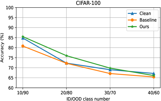
Figure 5: The performance of FixMatch [6], Clean and our method against four different ID/OOD ratios on CIFAR-100.

5.5 Robustness Against ID/OOD Ratios

To demonstrate the robustness of our method against different ratios of ID/OOD samples in the training dataset, we test our method against the FixMatch [6] baseline and its “Clean” variant on CIFAR-100 [11] dataset against four different ID/OOD ratios: 10/90, 20/80, 30/70 and 40/60. We report the average performance over three runs. As Fig. 5 shows, our method outperforms the FixMatch baseline in all four settings and achieves higher accuracy than the Clean model in three settings: 10/90, 20/80 and 30/70. Such a constant improvement justifies the robustness of our method against different ID/OOD ratios. Note that the degradation of performance in all three models is caused by the increasing ID class number.

5.6 Performance on ID/OOD Classification

Following previous studies[42], we also compare the performance of our method with those of previous open-set semi-supervised learning methods on ID/OOD classification. The experiments are conducted on CIFAR-100 with two different settings and the AUROC values of each method are shown in Table V. As shown in the table, despite the imbalance between ID and OOD samples, our method achieves a significant improvement over previous methods. Please note that we use the output probabilities of the predicted class as ID probabilities to compute the AUROC value of FixMatch.

TABLE VI: The performance of our method against different numbers of pools (DomainNet-Real 20/50k).

No. of Pools	0	1	2	3	4
Our Method	52.5	53.2	54.3	52.2	50.8

TABLE VII: The performance of our method against different $N_{id}$ (DomainNet-Real 20/50k).

$N_{id}$	5	6	7	8	9
Our Method	53.8	54.3	54.0	53.1	52.6

5.7 Justification of our Choice on No. of Pools

To justify our choice of using a cascade of two pools in importance-based sampling, we investigate how the number of pools influences the performance of our method (Table VI). All other hyperparameters are kept the same across all experiments. It can be observed that: i) using two pools achieves the best performance; ii) when using zero or one pool, the density of ID samples is not high enough and thus worsens the minibatch training; iii) when using three or four pools, the density is improved but at the cost of filtering out too many unlabeled (ID) samples, which yields overfitting and also worsens the training. Thus, we use a cascade of two pools in our importance-based sampling implementation.

5.8 Threshold of ID/OOD Identification

The ID/OOD identification of our method selects $N_{id}$ prototypes that are closest to the feature center of labeled samples as ID prototypes. To investigate the influence of $N_{id}$ selection, we test our method on DomainNet-Real 20/50k and the results are shown in Table VII. It can be observed that our method performs better than the baseline with different $N_{id}$ and the best performance is achieved at 6.

TABLE VIII: The performance of our method against the number of prototypes (CIFAR-100 10/90).

Prototypes Num	2	6	10	14	18
Our Method	83.3	84.4	85.5	84.0	83.7

5.9 Number of Prototypes

To investigate how the number of prototypes influences the performance of our method, we test different choices of it on the CIFAR-100 10/90 setting and show the results in Table VIII. It can be observed that our method is insensitive to the number of prototypes and almost always outperforms the baseline (FixMatch [6]). Thus, we suggest to set the default value of it as $10$ (as used in this paper).

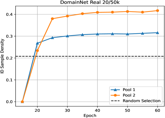
Figure 6: Justification of ID sample refinement (DomainNet -Real 20/50k). The ID sample density of our ID sample pools are much higher than that of the raw unlabeled dataset (Random Selection).

5.10 Effectiveness of Cascading Pools

To further justify the effectiveness of our cascading pooling strategy, we plot the density of ID samples in our two cascaded ID sample pools (with per-class capacity 300 and 150 respectively) against training epochs when training our model with the DomainNet-Real 20/50k setting (Figure 6). We also marked the percentage of ID samples in the raw unlabeled dataset as “Random Selection”. It can be observed that: i) Our two pools have much higher ID sample densities than Random Selection (approximately 10% and 20% respectively), which justifies the usefulness of our approach. ii) Pool 2 has a much higher ID sample density than Pool 1 (approximately 10%), which indicates the effectiveness of our cascading pooling strategy.

5.11 Performance on Fine-grained Classification

Fine-grained classification[45, 46, 47, 48, 49] aims to distinguish between objects that previously belong to the same (coarse-level) class, e.g., species of birds. Recently, there have been some studies that apply open-set semi-supervised learning on fine-grained classification[50], whose datasets contain both ID and OOD data. This is a more challenging task as samples in fine-grained classes (e.g., different brands of cars) have less discriminative features. In this section, we verify the effectiveness of our method on fine-grained classification.

Datasets. Following previous studies[50], we evaluate our method on two fine-grained datasets that exhibit a long-tailed distribution of classes and contain a large number of out-of-class images: Semi-Aves (from the semi-supervised challenge at FGVC7 workshop[51]) and Semi-Fungi (from the FGVC fungi challenge[52]). The OOD images of both datasets are those that do not belong to the classes of the labeled set. Between them, Semi-Aves contains 200 ID classes and 800 OOD classes, and 6K/27K/122K images in labeled set/ID unlabeled set/OOD unlabeled set, respectively. Semi-Fungi contains 200 ID classes and 1194 OOD classes, and 4K/13K/65K images in labeled set/ID unlabeled set/OOD unlabeled set, respectively. Following [50], we use the labeled and unlabeled set (containing both ID and OOD samples) provided by these datasets and ResNet-50[44] as the backbone network for evaluation. All samples are resized to a resolution of 224$\times$224 in all experiments.

Comparison Setup. Following[50], we compare our method to the following competitors: i) Supervised baseline, where the model is trained only on the labeled set; ii) Pseudo-Labeling[3], which uses a base model’s confident prediction on unlabeled images as pseudo-labels, and then trains a new model by sampling half of the batch from labeled data and half from pseudo-labeled data; iii) Curriculum Pseudo-Labeling[53], which repeats the following for 5 times: training a supervised model with labeled data, and expanding labeled data by including ($\{20,40,60,80,100\}\%$ of) the unlabeled data with the highest predictions. iv) FixMatch[6]; v) Self-Training, which first trains a teacher model with the labeled set, and then trains a student model with a scaled cross-entropy loss on the unlabeled data and a cross-entropy loss on the labeled data. vi) Supervised Oracle, which trains the model with the labeled set and ID unlabeled set with ground-truth labels.

As shown in Table IX and Table X, our method significantly outperforms all previous methods, which demonstrates the effectiveness of our method on fine-grained classification.

TABLE IX: Results on Semi-Aves benchmark. We experiment with six different SSL methods as well as supervised baselines. Results of other methods are copied from [50].

Method	Top-1	Top-5
Supervised baseline	20.6±0.4	41.7±0.7
Pseudo-Label[3]	12.2±0.8	31.9±1.6
Curriculum Pseudo-Label[53]	20.2±0.5	41.0±0.9
FixMatch[6]	19.2±0.2	42.6±0.6
Self-Training	22.0±0.5	43.3±0.2
Ours	26.9±0.5	48.4±0.8
Supervised oracle	57.4±0.3	79.2±0.1

TABLE X: Results on Semi-Fungi benchmark. We experiment with six different SSL methods as well as supervised baselines. Results of other methods are copied from [50].

Method	Top-1	Top-5
Supervised baseline	31.0±0.4	54.7±0.8
Pseudo-Label[3]	15.2±1.0	40.6±1.2
Curriculum Pseudo-Label[53]	30.8±0.1	54.4±0.3
FixMatch[6]	25.2±0.3	50.2±0.8
Self-Training	32.5±0.5	56.3±0.3
Ours	34.4±0.4	58.0±0.8
Supervised oracle	60.2±0.8	83.3±0.9

5.12 Visualization of ID/OOD Features

In this section, we apply our method to CIFAR10 for feature visualization. To better illustrate the difference and distribution of ID/OOD features, we select all 10 classes in CIFAR10[11] rather than datasets with more categories in our experiment. We set the first 5 classes in CIFAR10 as ID and other 5 classes as OOD. The feature visualization is shown in Fig 7, including the visualization of both baseline (FixMatch) and our method. As shown in Fig 7(a), baseline model can not separate the ID and OOD features and thus confuses the OOD detector. However, in Fig 7(b), our method can better cluster both ID/OOD features and thus preserves the difference between ID and OOD features in the feature level. Therefore, our method facilitates the training of the feature extractor and the ID/OOD classification in the importance-based sampling.

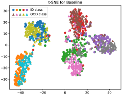
(a)

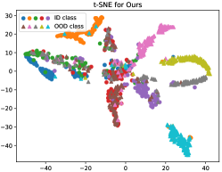
(b)

Figure 7: The t-SNE feature visualization on CIFAR-10. (a) provides the feature visualization of FixMatch. (b) shows the t-SNE results of our method. As shown in the figures, our method organizes both ID and OOD features and improves the feature extractor.

6 Conclusion

In this paper, we find that the proper use of OOD samples can benefit semi-supervised learning (SSL). Accordingly, we propose two techniques for open-set SSL: i) a prototype-based clustering and identification algorithm and ii) an importance-based sampling method. Our prototype-based clustering and identification algorithm clusters samples at feature-level and thus achieves better identification of ID and OOD samples by increasing their distances in-between. Addressing the sampling bias introduced by the ID/OOD identification process, we propose an importance-based sampling method that maintains a pyramid of sample pools containing samples that are important to SSL. We implemented our method on top of FixMatch [6] and achieved state-of-the-art in open-set SSL on extensive public benchmarks.

Ganlong Zhao received the BEng and MS degrees from the School of Computer Science and Engineering of Sun Yat-Sen University in 2019 and 2021 respectively. He is currently working toward the PhD degree in the Department of Computer Science at The University of Hong Kong. He worked as a research intern at Meituan Inc., in 2020. His research interests include machine learning and computer vision, specifically semi-supervised and unsupervised learning.

Guanbin Li (M’15) is currently an associate professor in School of Data and Computer Science, Sun Yat-sen University. He received his PhD degree from the University of Hong Kong in 2016. His current research interests include computer vision, image processing, and deep learning. He is a recipient of ICCV 2019 Best Paper Nomination Award. He has authorized and co-authorized on more than 100 papers in top-tier academic journals and conferences. He serves as an area chair for the conference of VISAPP. He has been serving as a reviewer for numerous academic journals and conferences such as TPAMI, IJCV, TIP, TMM, TCyb, CVPR, ICCV, ECCV and NeurIPS.

Yipeng Qin received the BS degree from Shanghai Jiaotong University in 2013, and the PhD degree from National Centre for Computer Animation (NCCA), Bournemouth University in 2017. From 2017 to 2019 he was a Postdoctoral Research Fellow at the Visual Computing Center (VCC), King Abdullah University of Science and Technology (KAUST). He joined the School of Computer Science and Informatics, Cardiff University, in 2019 as a lecturer. His current research interests include machine learning, computer vision and computer graphics.

Jinjin Zhang obtained M.Eng. in computer science from Beihang University in 2017 and B.E. degree from Changchun University of Science and Technology in 2013. He is now a senior computer vision engineer in Meituan. His research interests include self-supervised learning, semi-supervised learning and its applications to computer vision.

Zhenhua Chai received the B.E. (Hons.) degree in automation from the Central University of Nationality and the Ph.D. degree in computer application technology from the National Lab of Pattern Recognition, Institute of Automation, Chinese Academy of Sciences in 2008 and 2013, respectively. His research interests focus on AutoDL, model compression, self supervised learning and applications on face analysis. Currently he works as a research expert in Meituan.

Xiaolin Wei received Ph.D. in Computer Science from Texas A&M University. His research area includes computer vision, machine learning, computer graphics, 3D vision, augmented reality. He worked as a research engineer at Google, Virtroid and Magic Leap, and now is working at Meituan AI Lab.

Liang Lin (M’09, SM’15) is a full Professor of Sun Yat-sen University. He is an Excellent Young Scientist of the National Natural Science Foundation of China. From 2008 to 2010, he was a Post-Doctoral Fellow at the University of California, Los Angeles. From 2014 to 2015, as a senior visiting scholar, he was with The Hong Kong Polytechnic University and The Chinese University of Hong Kong. He currently leads the SenseTime R$\&$D teams to develop cutting-edge and deliverable solutions on computer vision, data analysis and mining, and intelligent robotic systems. He has authored and co-authored more than 100 papers in top-tier academic journals and conferences. He has been serving as an associate editor of IEEE Trans. Human-Machine Systems, The Visual Computer and Neurocomputing. He served as area/session chairs for numerous conferences, such as ICME, ACCV, ICMR. He was the recipient of the Best Paper Runners-Up Award in ACM NPAR 2010, the Google Faculty Award in 2012, the Best Paper Diamond Award in IEEE ICME 2017, and the Hong Kong Scholars Award in 2014. He is a Fellow of IET.

Yizhou Yu received the PhD degree from University of California at Berkeley in 2000. He is currently a professor at The University of Hong Kong, and was a faculty member at University of Illinois, Urbana-Champaign between 2000 and 2012. He is a recipient of 2002 US National Science Foundation CAREER Award, and 2007 NNSF China Overseas Distinguished Young Investigator Award. He has served on the editorial board of IET Computer Vision, IEEE Transactions on Visualization and Computer Graphics, The Visual Computer, and International Journal of Software and Informatics. He has also served on the program committee of many leading international conferences, including SIGGRAPH, SIGGRAPH Asia, and International Conference on Computer Vision. His current research interests include deep learning methods for computer vision, computational visual media, geometric computing, video analytics and biomedical data analysis.

References

- [1] M. Sajjadi, M. Javanmardi, and T. Tasdizen, “Regularization with stochastic transformations and perturbations for deep semi-supervised learning,” Advances in Neural Information Processing Systems, vol. 29, 2016.
- [2] S. Laine and T. Aila, “Temporal ensembling for semi-supervised learning,” in International Conference on Learning Representations, 2017.
- [3] D.-H. Lee et al., “Pseudo-label: The simple and efficient semi-supervised learning method for deep neural networks,” in Workshop on challenges in representation learning, ICML, vol. 3, no. 2, 2013.
- [4] H. Pham, Z. Dai, Q. Xie, and Q. V. Le, “Meta pseudo labels,” in Proceedings of the IEEE/CVF Conference on Computer Vision and Pattern Recognition, 2021, pp. 11 557–11 568.
- [5] Y. Grandvalet and Y. Bengio, “Semi-supervised learning by entropy minimization,” Advances in Neural Information Processing Systems, vol. 17, 2004.
- [6] K. Sohn, D. Berthelot, N. Carlini, Z. Zhang, H. Zhang, C. A. Raffel, E. D. Cubuk, A. Kurakin, and C.-L. Li, “Fixmatch: Simplifying semi-supervised learning with consistency and confidence,” Advances in Neural Information Processing Systems, vol. 33, pp. 596–608, 2020.
- [7] Q. Yu, D. Ikami, G. Irie, and K. Aizawa, “Multi-task curriculum framework for open-set semi-supervised learning,” in European Conference on Computer Vision. Springer, 2020, pp. 438–454.
- [8] S. Liang, Y. Li, and R. Srikant, “Enhancing the reliability of out-of-distribution image detection in neural networks,” in International Conference on Learning Representations, 2018.
- [9] D. Berthelot, N. Carlini, I. Goodfellow, N. Papernot, A. Oliver, and C. A. Raffel, “Mixmatch: A holistic approach to semi-supervised learning,” Advances in Neural Information Processing Systems, vol. 32, 2019.
- [10] J. Winkens, R. Bunel, A. G. Roy, R. Stanforth, V. Natarajan, J. R. Ledsam, P. MacWilliams, P. Kohli, A. Karthikesalingam, S. Kohl et al., “Contrastive training for improved out-of-distribution detection,” arXiv preprint arXiv:2007.05566, 2020.
- [11] A. Krizhevsky, G. Hinton et al., “Learning multiple layers of features from tiny images,” 2009.
- [12] Y. Netzer, T. Wang, A. Coates, A. Bissacco, B. Wu, and A. Y. Ng, “Reading digits in natural images with unsupervised feature learning,” 2011.
- [13] J. Deng, W. Dong, R. Socher, L.-J. Li, K. Li, and L. Fei-Fei, “Imagenet: A large-scale hierarchical image database,” in 2009 IEEE Conference on Computer Vision and Pattern Recognition. Ieee, 2009, pp. 248–255.
- [14] X. Peng, Q. Bai, X. Xia, Z. Huang, K. Saenko, and B. Wang, “Moment matching for multi-source domain adaptation,” in Proceedings of the IEEE/CVF International Conference on Computer Vision, 2019, pp. 1406–1415.
- [15] P. Bachman, O. Alsharif, and D. Precup, “Learning with pseudo-ensembles,” Advances in Neural Information Processing Systems, vol. 27, 2014.
- [16] X. Zhai, A. Oliver, A. Kolesnikov, and L. Beyer, “S4l: Self-supervised semi-supervised learning,” in Proceedings of the IEEE/CVF International Conference on Computer Vision, 2019, pp. 1476–1485.
- [17] S. Park, J. Park, S.-J. Shin, and I.-C. Moon, “Adversarial dropout for supervised and semi-supervised learning,” in Proceedings of the AAAI Conference on Artificial Intelligence, vol. 32, no. 1, 2018.
- [18] S. Wager, S. Wang, and P. S. Liang, “Dropout training as adaptive regularization,” Advances in Neural Information Processing Systems, vol. 26, 2013.
- [19] D. Berthelot, N. Carlini, E. D. Cubuk, A. Kurakin, K. Sohn, H. Zhang, and C. Raffel, “Remixmatch: Semi-supervised learning with distribution matching and augmentation anchoring,” in International Conference on Learning Representations, 2019.
- [20] A. Tarvainen and H. Valpola, “Mean teachers are better role models: Weight-averaged consistency targets improve semi-supervised deep learning results,” Advances in Neural Information Processing Systems, vol. 30, 2017.
- [21] B. Zhang, Y. Wang, W. Hou, H. Wu, J. Wang, M. Okumura, and T. Shinozaki, “Flexmatch: Boosting semi-supervised learning with curriculum pseudo labeling,” Advances in Neural Information Processing Systems, vol. 34, pp. 18 408–18 419, 2021.
- [22] J. Li, P. Zhou, C. Xiong, and S. Hoi, “Prototypical contrastive learning of unsupervised representations,” in International Conference on Learning Representations, 2020.
- [23] T. DeVries and G. W. Taylor, “Learning confidence for out-of-distribution detection in neural networks,” arXiv preprint arXiv:1802.04865, 2018.
- [24] Y. Ming, Z. Cai, J. Gu, Y. Sun, W. Li, and Y. Li, “Delving into out-of-distribution detection with vision-language representations,” in Advances in Neural Information Processing Systems, 2022.
- [25] X. Du, G. Gozum, Y. Ming, and Y. Li, “Siren: Shaping representations for detecting out-of-distribution objects,” in Advances in Neural Information Processing Systems, 2022.
- [26] J. Yang, P. Wang, D. Zou, Z. Zhou, K. Ding, W. PENG, H. Wang, G. Chen, B. Li, Y. Sun et al., “Openood: Benchmarking generalized out-of-distribution detection,” in Thirty-sixth Conference on Neural Information Processing Systems Datasets and Benchmarks Track.
- [27] C. Chow, “On optimum recognition error and reject tradeoff,” IEEE Transactions on information theory, vol. 16, no. 1, pp. 41–46, 1970.
- [28] P. Vincent and Y. Bengio, “Manifold parzen windows,” Advances in Neural Information Processing Systems, pp. 849–856, 2003.
- [29] A. Ghoting, S. Parthasarathy, and M. E. Otey, “Fast mining of distance-based outliers in high-dimensional datasets,” Data Mining and Knowledge Discovery, vol. 16, no. 3, pp. 349–364, 2008.
- [30] D. Hendrycks and K. Gimpel, “A baseline for detecting misclassified and out-of-distribution examples in neural networks,” in International Conference on Learning Representations, 2017.
- [31] K. Lee, K. Lee, H. Lee, and J. Shin, “A simple unified framework for detecting out-of-distribution samples and adversarial attacks,” Advances in neural information processing systems, vol. 31, 2018.
- [32] W. Liu, X. Wang, J. Owens, and Y. Li, “Energy-based out-of-distribution detection,” Advances in Neural Information Processing Systems, vol. 33, pp. 21 464–21 475, 2020.
- [33] Y.-C. Hsu, Y. Shen, H. Jin, and Z. Kira, “Generalized odin: Detecting out-of-distribution image without learning from out-of-distribution data,” in Proceedings of the IEEE/CVF Conference on Computer Vision and Pattern Recognition, 2020, pp. 10 951–10 960.
- [34] Y. Sun, C. Guo, and Y. Li, “React: Out-of-distribution detection with rectified activations,” in Advances in Neural Information Processing Systems, 2021.
- [35] A. Oliver, A. Odena, C. A. Raffel, E. D. Cubuk, and I. Goodfellow, “Realistic evaluation of deep semi-supervised learning algorithms,” Advances in Neural Information Processing Systems, vol. 31, 2018.
- [36] H. Luo, H. Cheng, Y. Gao, K. Li, M. Zhang, F. Meng, X. Guo, F. Huang, and X. Sun, “On the consistency training for open-set semi-supervised learning,” arXiv preprint arXiv:2101.08237, 2021.
- [37] Q. Xie, Z. Dai, E. Hovy, T. Luong, and Q. Le, “Unsupervised data augmentation for consistency training,” in Advances in Neural Information Processing Systems, H. Larochelle, M. Ranzato, R. Hadsell, M. F. Balcan, and H. Lin, Eds., vol. 33. Curran Associates, Inc., 2020, pp. 6256–6268.
- [38] Y. Chen, X. Zhu, W. Li, and S. Gong, “Semi-supervised learning under class distribution mismatch,” in Proceedings of the AAAI Conference on Artificial Intelligence, vol. 34, no. 04, 2020, pp. 3569–3576.
- [39] J. Huang, C. Fang, W. Chen, Z. Chai, X. Wei, P. Wei, L. Lin, and G. Li, “Trash to treasure: Harvesting ood data with cross-modal matching for open-set semi-supervised learning,” in Proceedings of the IEEE/CVF International Conference on Computer Vision, 2021, pp. 8310–8319.
- [40] T. Chen, S. Kornblith, M. Norouzi, and G. Hinton, “A simple framework for contrastive learning of visual representations,” in International Conference on Machine Learning. PMLR, 2020, pp. 1597–1607.
- [41] L.-Z. Guo, Z.-Y. Zhang, Y. Jiang, Y.-F. Li, and Z.-H. Zhou, “Safe deep semi-supervised learning for unseen-class unlabeled data,” in International Conference on Machine Learning. PMLR, 2020, pp. 3897–3906.
- [42] K. Saito, D. Kim, and K. Saenko, “Openmatch: Open-set consistency regularization for semi-supervised learning with outliers,” in Advances in Neural Information Processing Systems, 2021.
- [43] S. Zagoruyko and N. Komodakis, “Wide residual networks,” in British Machine Vision Conference 2016. British Machine Vision Association, 2016.
- [44] K. He, X. Zhang, S. Ren, and J. Sun, “Deep residual learning for image recognition,” in Proceedings of the IEEE conference on Computer Vision and Pattern Recognition, 2016, pp. 770–778.
- [45] Z. Akata, S. Reed, D. Walter, H. Lee, and B. Schiele, “Evaluation of output embeddings for fine-grained image classification,” in Proceedings of the IEEE conference on computer vision and pattern recognition, 2015, pp. 2927–2936.
- [46] Z. Yang, T. Luo, D. Wang, Z. Hu, J. Gao, and L. Wang, “Learning to navigate for fine-grained classification,” in Proceedings of the European Conference on Computer Vision (ECCV), 2018, pp. 420–435.
- [47] A. Dubey, O. Gupta, R. Raskar, and N. Naik, “Maximum-entropy fine grained classification,” Advances in neural information processing systems, vol. 31, 2018.
- [48] T. Syeda-Mahmood, K. C. Wong, Y. Gur, J. T. Wu, A. Jadhav, S. Kashyap, A. Karargyris, A. Pillai, A. Sharma, A. B. Syed et al., “Chest x-ray report generation through fine-grained label learning,” in International Conference on Medical Image Computing and Computer-Assisted Intervention. Springer, 2020, pp. 561–571.
- [49] Y. Zhu, X. Deng, and S. Newsam, “Fine-grained land use classification at the city scale using ground-level images,” IEEE Transactions on Multimedia, vol. 21, no. 7, pp. 1825–1838, 2019.
- [50] J.-C. Su, Z. Cheng, and S. Maji, “A realistic evaluation of semi-supervised learning for fine-grained classification,” in Proceedings of the IEEE/CVF Conference on Computer Vision and Pattern Recognition, 2021, pp. 12 966–12 975.
- [51] J.-C. Su and S. Maji, “The semi-supervised inaturalist-aves challenge at fgvc7 workshop,” arXiv preprint arXiv:2103.06937, 2021.
- [52] 2018 FGVCx Fungi Classification Challenge, https://github.com/visipedia/fgvcx_fungi_comp.
- [53] P. Cascante-Bonilla, F. Tan, Y. Qi, and V. Ordonez, “Curriculum labeling: Revisiting pseudo-labeling for semi-supervised learning,” in Proceedings of the AAAI Conference on Artificial Intelligence, vol. 35, no. 8, 2021, pp. 6912–6920.