Thompson Sampling for Improved Exploration in GFlowNets

Abstract

Generative flow networks (GFlowNets) are amortized variational inference algorithms that treat sampling from a distribution over compositional objects as a sequential decision-making problem with a learnable action policy. Unlike other algorithms for hierarchical sampling that optimize a variational bound, GFlowNet algorithms can stably run off-policy, which can be advantageous for discovering modes of the target distribution. Despite this flexibility in the choice of behaviour policy, the optimal way of efficiently selecting trajectories for training has not yet been systematically explored. In this paper, we view the choice of trajectories for training as an active learning problem and approach it using Bayesian techniques inspired by methods for multi-armed bandits. The proposed algorithm, Thompson sampling GFlowNets (TS-GFN), maintains an approximate posterior distribution over policies and samples trajectories from this posterior for training. We show in two domains that TS-GFN yields improved exploration and thus faster convergence to the target distribution than the off-policy exploration strategies used in past work.

1 Introduction

Generative flow networks (GFlowNets; Bengio et al., 2021) are generative models which sequentially construct objects from a space $\mathcal{X}$ by taking a series of actions sampled from a learned policy $P_{F}$. A GFlowNet’s policy $P_{F}$ is trained such that, at convergence, the probability of obtaining some object $x\in\mathcal{X}$ as the result of sampling a sequence of actions from $P_{F}$ is proportional to a reward $R(x)$ associated to $x$. Whereas traditional probabilistic modeling approaches (e.g., those based on Markov chain Monte Carlo (MCMC)) rely on local exploration in $\mathcal{X}$ for good performance, the parametric policy learned by GFlowNets allows them to generalize across states and yield superior performance on a number of tasks (Bengio et al., 2021; Malkin et al., 2022; Zhang et al., 2022; Jain et al., 2022a; Deleu et al., 2022; Jain et al., 2022b; Hu et al., 2023; Zhang et al., 2023).

While GFlowNets solve the variational inference problem of approximating a target distribution on $\mathcal{X}$ with the distribution induced by the sampling policy (Malkin et al., 2023), they are trained in a manner reminiscent of reinforcement learning (RL). GFlowNets are typically trained by either sampling trajectories on-policy from the learned sampling policy or off-policy from a mix of the learned policy and random noise. Each trajectory sampled concludes with some object $x\in\mathcal{X}$ for which the GFlowNet receives reward $R(x)$ and takes a gradient step on the parameters of the sampler with respect to the reward signal. Despite GFlowNets’ prior successes, this mode of training leaves them vulnerable to issues seen in the training of reinforcement learning agents — namely, slow temporal credit assignment and optimally striking the balance between exploration and exploitation.

Although multiple works have tackled the credit assignment issue in GFlowNets (Malkin et al., 2022; Madan et al., 2023; Deleu et al., 2022; Pan et al., 2023), considerably less attention has been paid to the exploration problem. Recently Pan et al. (2022) proposed to augment GFlowNets with intermediate rewards so as to allow the addition of intrinsic rewards (Pathak et al., 2017; Burda et al., 2018) and incorporate an exploration signal directly into training. However, while density-based exploration bonuses can provide much better performance on tasks where the reward $R(x)$ is very sparse, there is no guarantee that the density-based incentives correlate with model uncertainty or task structure. In fact, they have been shown to yield arbitrarily poor performance in a number of reinforcement learning settings (Osband et al., 2019). In this paper, we develop an exploration method for GFlowNets which provides improved convergence to the target distribution even when the reward $R(x)$ is not sparse.

Thompson sampling (TS; Thompson, 1933) is a method which provably manages the exploration/exploitation problem in settings from multi-armed bandits to reinforcement learning (Agrawal & Jia, 2017; Agrawal & Goyal, 2017) and has been employed to much success across a variety of deep reinforcement learning tasks (Osband et al., 2016a, 2018, 2019). The classical TS algorithm (Agrawal & Goyal, 2012; Russo et al., 2018) maintains a posterior over the model of the environment and acts optimally according to a sample from this posterior over models. TS has been generalized to RL problems in the form of Posterior Sampling RL (Osband et al., 2013). A variant of TS has been adapted in RL, where the agent maintains a posterior over policies and value functions (Osband et al., 2016b, a) and acts optimally based on a random sample from this posterior. We consider this variant of TS in this paper.

Our main contribution in this paper is describing and evaluating an algorithm based on Thompson sampling for improved exploration in GFlowNets. Building upon prior results in Malkin et al. (2022); Madan et al. (2023) we demonstrate how Thompson sampling with GFlowNets allows for improved exploration and optimization efficiency in GFlowNets. We validate our method on a grid-world and sequence generation task. In our experiments TS-GFN substantially improves both the sample efficiency and the task performance. Our algorithm is computationally efficient and highly parallelizable, only taking $\sim 15\%$ more computation time than prior approaches.

2 Related Work

Exploration in RL

There exists a wide literature on uncertainty based RL exploration methods. Some methods rely on the Thompson sampling heuristic and non-parametric representations of the posterior to promote exploration (Osband et al., 2013, 2016a, 2016b, 2018). Others employ uncertainty to enable exploration based on the upper confidence bound heuristic or information gain (Ciosek et al., 2019; Lee et al., 2021; O’Donoghue et al., 2018; Nikolov et al., 2018). Another set of exploration methods attempts to make agents “intrinsically” motivated to explore. This family of methods includesrandom network distillation (RND) and Never Give Up (Burda et al., 2018; Badia et al., 2020). Pan et al. (2022), proposes to augment GFlowNets with intrinsic RND-based intrinsic rewards to encourage better exploration.

MaxEnt RL

RL has a rich literature on energy-based, or maximum entropy, methods (Ziebart, 2010; Mnih et al., 2016; Haarnoja et al., 2017; Nachum et al., 2017; Schulman et al., 2017; Haarnoja et al., 2018), which are close or equivalent to the GFlowNet framework in certain settings (in particular when the MDP has a tree structure (Bengio et al., 2021)). Also related are methods that maximize entropy of the state visitation distribution or some proxy of it (Hazan et al., 2019; Islam et al., 2019; Zhang et al., 2021; Eysenbach et al., 2018), which achieve a similar objective to GFlowNets by flattening the state visitation distribution. We hypothesize that even basic exploration methods for GFlowNets (e.g., tempering or $\epsilon$-noisy) could be sufficient exploration strategies on some tasks.

3 Method

3.1 Preliminaries

We begin by summarizing the preliminaries on GFlowNets, following the conventions of Malkin et al. (2022).

Let $G=(\mathcal{S},\mathcal{A})$ be a directed acyclic graph. The vertices $s\in\mathcal{S}$ are called states and the directed edges $(u\rightarrow v)\in\mathcal{A}$ are actions. If $(u\rightarrow v)$ is an edge, we say $v$ is a child of $u$ and $u$ is a parent of $v$. There is a unique initial state $s_{0}\in\mathcal{S}$ with no parents. States with no children are called terminal, and the set of terminal states is denoted by $\mathcal{X}$.

A trajectory is a sequence of states $\tau=(s_{m}\rightarrow s_{m+1}\rightarrow\dots\rightarrow s_{n})$, where each $(s_{i}\rightarrow s_{i+1})$ is an action. The trajectory is complete if $s_{m}=s_{0}$ and $s_{n}$ is terminal. The set of complete trajectories is denoted by $\mathcal{T}$.

A (forward) policy is a collection of distributions $P_{F}(-|s)$ over the children of every nonterminal state $s\in\mathcal{S}$. A forward policy determines a distribution over $\mathcal{T}$ by

$$P_{F}(\tau=(s_{0}\rightarrow\dots\rightarrow s_{n}))=\prod_{i=0}^{n-1}P_{F}(s_{i+1}|s_{i}).$$ (1)

Similarly, a backward policy is a collection of distributions $P_{B}(-|s)$ over the parents of every noninitial state.

Any distribution over complete trajectories that arises from a forward policy satisfies a Markov property: the marginal choice of action out of a state $s$ is independent of how $s$ was reached. Conversely, any Markovian distribution over $\mathcal{T}$ arises from a forward policy (Bengio et al., 2023).

A forward policy can thus be used to sample terminal states $x\in\mathcal{X}$ by starting at $s_{0}$ and iteratively sampling actions from $P_{F}$, or, equivalently, taking the terminating state of a complete trajectory $\tau\sim P_{F}(\tau)$. The marginal likelihood of sampling $x\in\mathcal{X}$ is the sum of likelihoods of all complete trajectories that terminate at $x$.

Suppose that a nontrivial (not identically 0) nonnegative reward function $R:\mathcal{X}\to\mathbb{R}_{\geq 0}$ is given. The learning problem solved by GFlowNets is to estimate a policy $P_{F}$ such that the likelihood of sampling $x\in\mathcal{X}$ is proportional to $R(x)$. That is, there should exist a constant $Z$ such that

$$R(x)=Z\sum_{\tau in\mathcal{T}:\tau=(s_{0}\rightarrow\dots\rightarrow s_{n}=x)}P_{F}(\tau)\quad\forall x\in\mathcal{X}.$$ (2)

If (2) is satisfied, then $Z=\sum_{x\in\mathcal{X}}R(x)$. The sum in (2) may be intractable. Therefore, GFlowNet training algorithms require estimation of auxiliary quantities beyond the parameters of the policy $P_{F}$. The training objective we primarily consider, trajectory balance (TB), learns an estimate of the constant $Z$ and of a backward policy, $P_{B}(s\mid s^{\prime})$, representing the posterior over predecessor states of $s^{\prime}$ in trajectories that contain $s^{\prime}$. The TB loss for a trajectory $\tau$ is:

$$\mathcal{L}_{TB}(\tau;\theta)=\left(\log\frac{Z_{\theta}\prod_{t=0}^{n-1}P_{F}(s_{t+1}|s_{t};\theta)}{R(s_{n})\prod_{t=0}^{n-1}P_{B}(s_{t}|s_{t+1};\theta)}\right)^{2}$$ (3)

where $\theta$ are the parameters of the learned objects $P_{F}$, $P_{B}$, and $Z$. If $\mathcal{L}_{TB}(\tau;\theta)=0$ for all $\tau$, then $P_{F}$ samples objects $x\in\mathcal{X}$ with probability proportional to $R(x)$, i.e., (2) is satisfied. Algorithms minimize this loss for trajectories $\tau$ sampled from some training policy $\pi_{\theta}$, which may be equal to $P_{F}$ itself (on-policy training) but is usually taken to be a more exploratory distribution, as we discuss below.

Notably, any choice of a backwards policy $P_{B}$ yields a unique corresponding $P_{F}$ and $Z$ which makes the expression on the right side of (3) equal to zero for all $\tau\in\mathcal{T}$ (see Malkin et al. (2023) for interpretations of this result in terms of variational methods).

3.2 GFlowNet exploration strategies

Prior work on GFlowNets uses training policies based on dithering or intrinsic motivation, including:

On-policy

The training policy is the current $P_{F}$: $\pi_{\theta}(s^{\prime}|s)=P_{F}(s^{\prime}|s;\theta)$.

Tempering

Let $\alpha_{\theta}(s^{\prime}|s):\mathcal{S}\times\mathcal{S}\rightarrow\mathbb{R}$ be the logits of $P_{F}$, then the training policy is a Boltzmann distribution with temperature $T\in\mathbb{R}$ as $\pi_{\theta}(s^{\prime}|s)\propto\exp\left(\alpha_{\theta}(s^{\prime}|s)/T\right)$.

$\epsilon$-noisy

For $\epsilon\in[0,1]$, the training policy follows $P_{F}$ with probability $1-\epsilon$ and takes a random action with probability $\epsilon$ as $\pi_{\theta}(s^{\prime}|s)=(1-\epsilon)P_{F}(s^{\prime}|s;\theta)+\frac{\epsilon}{\#\{s^{\prime\prime}:(s\rightarrow s^{\prime\prime})\in\mathcal{A}\}}$.

GAFN (Pan et al., 2022)

The training policy is the current $P_{F}$, but $P_{F}$ is learned by incorporating a pseudocount-based intrinsic reward for each state $s\in\tau$ into the objective $\mathcal{L}(\tau;P_{F},P_{B})$ so that $\pi_{\theta}(s^{\prime}|s)=P_{F}(s^{\prime}|s;\theta)$.

3.3 Thompson sampling for GFlowNets

Learning GFlowNets over large spaces $\mathcal{X}$ requires judicious exploration. It makes little sense to explore in regions the GFlowNet has already learned well – we would much rather prioritize exploring regions of the state space on which the GFlowNet has not accurately learned the reward distribution. Prior methods do not explicitly prioritize this. Both dithering approaches (tempering and $\epsilon$-noisy) and GAFNs encourage a form of uniform exploration, be it pure random noise as in dithering or a pseudocount in GAFNs. While it is impossible to a priori determine which regions a GFlowNet has learned poorly, we might expect that it performs poorly in the regions on which it is uncertain. An agent with an estimate of its own uncertainty could bias its action selection towards regions in which it is more uncertain.

With this intuition in mind, we develop an algorithm inspired by Thompson sampling and its applications in RL and bandits (Osband et al., 2016a, 2018). In particular, following Osband et al. (2016a) we maintain an approximate posterior over forward policies $P_{F}$ by viewing the last layer of our policy network itself as an ensemble. To maintain a size $K\in\mathbb{Z}^{+}$ ensemble extend the last layer of the policy network to have $K\cdot\ell$ heads where $\ell$ is the maximum number of valid actions according to $G$ for any state $s\in\mathcal{S}$. To promote computational efficiency all members of our ensemble share weights in all layers prior to the final one.

To better our method’s uncertainty estimates, we employ the statistical bootstrap to determine which trajectories $\tau$ may be used to train ensemble member $P_{F,k}$ and also make use of randomized prior networks (Osband et al., 2018). Prior networks are a downsized version of our main policy network whose weights are fixed at initialization and whose output is summed with the main network in order to produce the actual policy logits. Prior networks have been shown to significantly improve uncertainty estimates and agent performance in reinforcement learning tasks.

Crucially, while we parameterize an ensemble of $K$ forward policies we do not maintain an ensemble of backwards policies, instead sharing one $P_{B}$ across all ensemble members $P_{F,k}$. Recall from 3.1 that each $P_{B}$ uniquely determines a $P_{F}$ which $\mathcal{L}_{TB}(\tau)=0\quad\forall\tau\in\mathcal{T}$. Specifying a different $P_{B,k}$ for each $P_{F,k}$ would result in setting a different learning target for each $P_{F,k}$ in the ensemble. By sharing a single $P_{B}$ across all ensemble members we ensure that all $P_{F,k}$ converge to the same optimal $P_{F}^{*}$. We show in Section 4.1 that sharing $P_{B}$ indeed yields significantly better performance than maintaining separate $P_{B,k}$.

With our policy network parameterization in hand, the rest of our algorithm is simple. First we sample an ensemble member $P_{F,k}$ with $k\sim\textrm{Uniform}\{1,\dots,K\}$ and then sample an entire trajectory from it $\tau\sim P_{F,k}$. This trajectory is then used to train each ensemble member where we include the trajectory in the training batch for ensemble member $P_{F,k}$ based on the statistical bootstrap with bootstrap probability $p$ ($p$ is a hyperparameter fixed at the beginning of training). The full algorithm is presented in Appendix A.

4 Experiments

4.1 Grid

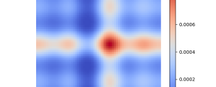
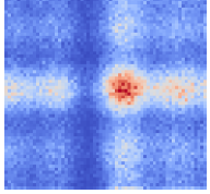
Figure 1: Reward on the grid task. Left: true distribution (normalized reward function). Right: empirical distribution over last $2\cdot 10^{5}$ states sampled from the GFlowNet at end of training.

We study a modified version of the grid environment from (Bengio et al., 2021). The set of interior states is a 2-dimensional grid of size $H\times H$. The initial state is $(0,0)$ and each action is a step that increments one of the 2 coordinates by 1 without leaving the grid. A special termination action is also allowed from each state.

Prior versions of this grid environment provide high reward whenever the agent exits at a corner of the grid. This sort of reward structure is very easy for an agent to generalize to and is a trivial exploration task when the reward is not highly sparse (such reward structures are not the focus of this paper). To compensate for this, we adopt a reward function based on a summation of truncated Fourier series, yielding a reward structure which is highly multimodal and more difficult to generalize to (see Figure 1). The reward function is given by

$$R(x)=\sum_{k=1}^{n} \cos(2a_{k,1}\pi g(x_{1}))+\sin(2a_{k,2}\pi g(x_{1}))+$$

$$\cos(2b_{k,1}\pi g(x_{2}))+\sin(2b_{k,2}\pi g(x_{2}))$$

where $a_{k,1},a_{k,2},b_{k,1},b_{k,2}\in\mathbb{R}$ are preset scaling constants $\forall k$, $n$ is a hyperparameter determining the number of elements in the summation, $g:\mathbb{Z}_{\geq 0}\rightarrow[c,d],g(x)=\frac{x(d-c)}{H}+c$, and $c,d\in\mathbb{R}$ are the first and last integer coordinates in the grid.

We investigate a $64\times 64$ grid with this truncated Fourier series reward (see Appendix B for full reward setup details). We train the GFlowNets to sample from this target reward function and plot the evolution of the $L_{1}$ distance between the target distribution and the empirical distribution of the last $2\cdot 10^{5}$ states seen in training.

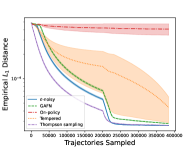
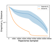
Figure 2: $L_{1}$ distance between empirical and target distributions over the course of training on the hypergrid environment (mean is plotted with standard error bars over 5 random seeds). Left: Thompson sampling learns the distribution better and faster than all other methods. Right: sharing a backwards policy $P_{B}$ performs significantly better than maintaining a separate backward policy $P_{B,k}$ for each forward policy $P_{F,k}$ in the ensemble.

The results (mean and standard error over five random seeds) are shown in Figure 2 (left side). Models trained with trajectories sampled by TS-GFN converge faster and with very little variance over random seeds to the true distribution than all other exploration strategies.

We also investigate the effect of sharing the backwards policy $P_{B}$ across ensemble members in Figure 2 (right side). Maintaining a separate $P_{B,k}$ for each $P_{F,k}$ performs significantly worse than sharing a single $P_{B}$ over all ensemble members. Maintaining separate $P_{B,k}$ resulted in the GFlowNet learning much slower than sharing $P_{B}$ and converging to a worse empirical $L_{1}$ than sharing $P_{B}$.

4.2 Bit sequences

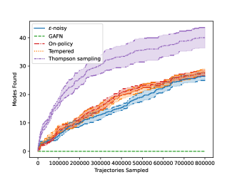
Figure 3: Number of modes found as a function of training time for bit sequence task.

We consider the synthetic sequence generation setting from Malkin et al. (2022), where the goal is to generate sequences of bits of fixed length $n=120$, resulting in a search space $\mathcal{X}$ of size $2^{120}$. The reward is specified by a set of modes $M\subset\mathcal{X}=\{0,1\}^{n}$ that is unknown to the learning agent. The reward of a generated sequence $x$ is defined in terms of Hamming distance $d$ from the modes: $R(x)=\exp\left(1-n^{-1}\min_{y\in M}d(x,y)\right)$. The vocabulary for the GFlowNets is $\{0,1\}$. Most experiment settings are taken from Malkin et al. (2022) and Madan et al. (2023).

Models are evaluated by tracking the number of modes according to the procedure in Malkin et al. (2022) wherein we count a mode $m$ as “discovered” if we sample some $x$ such that $d(x,m)\leq\delta$. The results are presented in Figure 3 (mean and standard error are plotted over five random seeds). We find that models trained with TS-GFN find  60% more modes than on-policy, tempering, and $\epsilon$-noisy. TS-GFN soundly outperforms GAFN, whose pseudocount based exploration incentive is misaligned with the task’s reward structure and seems to perform exploration in unhelpful regions of the (very large) search space.

5 Conclusion

We have shown in this paper that using a Thompson sampling based exploration strategy for GFlowNets is a simple, computationally efficient, and performant alternative to prior GFlowNet exploration strategies. We demonstrated how to adapt uncertainty estimation methods used for Thompson sampling in deep reinforcement learning to the GFlowNet domain and proved their efficacy on a grid and long sequence generation task. Finally, we believe that future work should involve trying TS-GFN on a wider array of experimental settings and building a theoretical framework for investigating sample complexity of GFlowNets.

Appendix A Additional algorithm details

  Input:

  $\{P_{F,k}\}_{k=1}^{K}$: Family of $K$ different forward policies 

  $P_{B}$: Shared backwards policy 

  $\delta\in[0,1]$: Parameter for the bootstrapping distribution (we assume the distribution is Bernoulli) 

  $L$: Loss function taking as input a trajectory $\tau$, forward policy $P_{F}$, and backward policy $P_{B}$

  for each episode do

     Initialize $s_{0}$ from environment

     Initialize trajectory $\tau$ to empty list

     Pick forward policy to act with $P_{F,k}$ using $k\sim\textrm{Uniform}\{1,\dots,K\}$

     for step $t=1,\dots$ until end of episode do

        Pick action $a_{t}\sim P_{F,k}(a_{t}|s_{t-1})$

        Receive state $s_{t}$ from environment

        Append $(s_{t},a_{t})$ to $\tau$

     end for

     Add reward for trajectory $R(x)$ to $\tau$ using last state in $\tau$

     Sample bootstrap mask $m_{k}\sim\textrm{Bernoulli}(\delta)\quad\forall k$

     Compute loss $\ell=\sum_{k=1}^{K}m_{k}\cdot L(\tau,P_{F,k},P_{B})$

     Take gradient step on loss $\ell$

  end for

Algorithm 1 TS-GFN

Appendix B Experiment details: Grid

For brevity, we recall the definition of the reward function from Section 4.1 as

$$R(x)=\sum_{k=1}^{n}\cos(2a_{k,1}\pi g(x_{1}))+\sin(2a_{k,2}\pi g(x_{1}))+\cos(2b_{k,1}\pi g(x_{2}))+\sin(2b_{k,2}\pi g(x_{2}))$$

The reward function was computed using the following hyperparameters. The weights were set as $a_{k,1}=a_{k,2}=b_{k,1}=b_{k,2}=\frac{4k}{1000}$ with $n=1000$ (the equivalent of np.linspace(0, 4, 1000)). The grid side boundary constants were $c=-0.5,d=0.5$ and the side length of the overall environment was $H=64$ (so that the overall state space was of size $H\times H=64^{2}=4096$). Finally, we raised the reward by the exponent $\beta=1.5$ so that we trained the GFlowNets using reward $R^{\prime}(x)=R(x)^{\beta}$.

Besides the reward, architecture details are identical to those in Malkin et al. (2022), Madan et al. (2023), and Bengio et al. (2021). The architecture of the forward and backward policy models are MLPs of the same architecture as in Bengio et al. (2021), taking a one-hot representation of the coordinates of $s$ as input and sharing all layers except the last. The only difference comes from the TS-GFN implementation which has $K\cdot d$ heads for the output of the last layer where $d$ is the number of heads in the architecture of the non-TS-GFNs.

All models are trained with the Adam optimizer, the trajectory balance loss, and a batch size of 64 for a total of $400,000$ trajectories. Hyperparameters were tuned using the Optuna Bayesian optimization framework from project Ray (Akiba et al., 2019; Moritz et al., 2018). Each method was allowed 100 hyperparameter samples from the Bayesian optimization procedure. We reported performance from the best hyperparameter setting found by the Bayesian optimization procedure averaged over five random seeds ($0,1,2,3,4$). We now detail the hyperparameters selected from the Bayesian optimization procedure for each exploration strategy.

For on-policy we found optimal hyperparameters of $0.00156$ for the model learning rate and $0.00121$ for the $\log Z$ learning rate. For tempering we found optimal hyperparameters of $0.00236$ for the model learning rate, $0.0695$ for the $\log Z$ learning rate, and $1.0458$ for the sampling policy temperature. For $\epsilon$-noisy we found optimal hyperparameters of $0.00112$ for the model learning rate, $0.0634$ for the $\log Z$ learning rate, and $0.00534$ for $\epsilon$. For GAFN we found optimal hyperparameters of $0.000166$ for the model learning rate, $0.0955$ for the $\log Z$ learning rate, $0.144$ for the intrinsic reward weight, and the architecture of the RND networks were a 2 layer MLP with hidden layer dimension of $53$ and output embedding dimension of $96$ (the hidden layer dimension and embedding dimension were also tuned by the Bayesian optimization procedure). Finally, for Thompson sampling we found a model learning rate of $0.00266$, $\log Z$ learning rate of $0.0976$, ensemble size of $100$, bootstrap probability $\delta$ of $0.274$, and prior weight of $12.03$.

Appendix C Experiment details: Bit sequences

The modes $M$ as well as the test sequences are selected as described in Malkin et al. (2022). The policy for all methods is parameterized by a Transformer (Vaswani et al., 2017) with 3 layers, dimension 64, and 8 attention heads. All methods are trained for 50,000 iterations with minibatch size of 16 using Adam optimizer and the trajectory balance loss.

All hyperparameters were tuned according to a grid search over the parameter values specified below. For on-policy we used a model learning rate of $0.0001$ picked from the set $\{0.0001,0.001,0.01\}$ and a $\log Z$ learning rate of $0.001$ from the set $\{0.001,0.01\}$. For tempering we used a model learning rate of $0.0001$ picked from the set $\{0.0001,0.001,0.01\}$, a $\log Z$ learning rate of $0.001$ from the set $\{0.001,0.01\}$, and sampling distribution temperature of $1.1$ from the set $\{1.05,1.1,1.25,1.5\}$. For $\epsilon$-noisy we used a learning rate of $0.001$ picked from the set $\{0.0001,0.001,0.01\}$, a $\log Z$ learning rate of $0.001$ from the set $\{0.001,0.01\}$, and $\epsilon$ of $0.005$ from the set $\{0.01,0.005,0.001,0.0005\}$. For GAFN we used a learning rate of $0.001$ picked from the set $\{0.0001,0.0005,0.001\}$, a $\log Z$ learning rate of $0.1$ from the set $\{0.001,0.01,0.1\}$, an intrinsic reward weight of $0.5$ from the set $\{0.1,0.5,1.0,5.0,10.0\}$, the RND network was a 4 layer MLP with hidden layer dimension of $64$ and output dimension of $64$. For TS-GFN we used a model learning rate of $0.001$ picked from the set $\{0.0001,0.001,0.01\}$, a $\log Z$ learning rate of $0.001$ from the set $\{0.001,0.01\}$, an ensemble size of $50$ picked from the set $\{10,50,100\}$, a prior weight of $4.0$ picked from the set $\{0.1,1.0,4.0\}$, and a bootstrap probability $\delta$ 0f $0.75$.

References

- Agrawal & Goyal (2012) Agrawal, S. and Goyal, N. Analysis of thompson sampling for the multi-armed bandit problem. In Conference on learning theory, pp. 39–1. JMLR Workshop and Conference Proceedings, 2012.
- Agrawal & Goyal (2017) Agrawal, S. and Goyal, N. Near-optimal regret bounds for thompson sampling. Journal of the ACM (JACM), 64(5):1–24, 2017.
- Agrawal & Jia (2017) Agrawal, S. and Jia, R. Optimistic posterior sampling for reinforcement learning: worst-case regret bounds. Advances in Neural Information Processing Systems, 30, 2017.
- Akiba et al. (2019) Akiba, T., Sano, S., Yanase, T., Ohta, T., and Koyama, M. Optuna: A next-generation hyperparameter optimization framework. In Proceedings of the 25th ACM SIGKDD international conference on knowledge discovery & data mining, pp. 2623–2631, 2019.
- Badia et al. (2020) Badia, A. P., Sprechmann, P., Vitvitskyi, A., Guo, D., Piot, B., Kapturowski, S., Tieleman, O., Arjovsky, M., Pritzel, A., Bolt, A., et al. Never give up: Learning directed exploration strategies. arXiv preprint arXiv:2002.06038, 2020.
- Bengio et al. (2021) Bengio, E., Jain, M., Korablyov, M., Precup, D., and Bengio, Y. Flow network based generative models for non-iterative diverse candidate generation. Neural Information Processing Systems (NeurIPS), 2021.
- Bengio et al. (2023) Bengio, Y., Lahlou, S., Deleu, T., Hu, E., Tiwari, M., and Bengio, E. GFlowNet foundations. arXiv preprint 2111.09266, 2023.
- Burda et al. (2018) Burda, Y., Edwards, H., Storkey, A., and Klimov, O. Exploration by random network distillation. arXiv preprint arXiv:1810.12894, 2018.
- Ciosek et al. (2019) Ciosek, K., Vuong, Q., Loftin, R., and Hofmann, K. Better exploration with optimistic actor critic. Advances in Neural Information Processing Systems, 32, 2019.
- Deleu et al. (2022) Deleu, T., Góis, A., Emezue, C., Rankawat, M., Lacoste-Julien, S., Bauer, S., and Bengio, Y. Bayesian structure learning with generative flow networks. Uncertainty in Artificial Intelligence (UAI), 2022.
- Eysenbach et al. (2018) Eysenbach, B., Gupta, A., Ibarz, J., and Levine, S. Diversity is all you need: Learning skills without a reward function. International Conference on Learning Representations (ICLR), 2018.
- Haarnoja et al. (2017) Haarnoja, T., Tang, H., Abbeel, P., and Levine, S. Reinforcement learning with deep energy-based policies. International Conference on Machine Learning (ICML), 2017.
- Haarnoja et al. (2018) Haarnoja, T., Zhou, A., Abbeel, P., and Levine, S. Soft actor-critic: Off-policy maximum entropy deep reinforcement learning with a stochastic actor. International Conference on Machine Learning (ICML), 2018.
- Hazan et al. (2019) Hazan, E., Kakade, S., Singh, K., and Van Soest, A. Provably efficient maximum entropy exploration. International Conference on Machine Learning (ICML), 2019.
- Hu et al. (2023) Hu, E. J., Malkin, N., Jain, M., Everett, K., Graikos, A., and Bengio, Y. GFlowNet-EM for learning compositional latent variable models. International Conference on Machine Learning (ICML), 2023.
- Islam et al. (2019) Islam, R., Ahmed, Z., and Precup, D. Marginalized state distribution entropy regularization in policy optimization. arXiv preprint 1912.05128, 2019.
- Jain et al. (2022a) Jain, M., Bengio, E., Hernandez-Garcia, A., Rector-Brooks, J., Dossou, B. F., Ekbote, C., Fu, J., Zhang, T., Kilgour, M., Zhang, D., Simine, L., Das, P., and Bengio, Y. Biological sequence design with GFlowNets. International Conference on Machine Learning (ICML), 2022a.
- Jain et al. (2022b) Jain, M., Raparthy, S. C., Hernandez-Garcia, A., Rector-Brooks, J., Bengio, Y., Miret, S., and Bengio, E. Multi-objective GFlowNets. arXiv preprint 2210.12765, 2022b.
- Lee et al. (2021) Lee, K., Laskin, M., Srinivas, A., and Abbeel, P. Sunrise: A simple unified framework for ensemble learning in deep reinforcement learning. In International Conference on Machine Learning, pp. 6131–6141. PMLR, 2021.
- Madan et al. (2023) Madan, K., Rector-Brooks, J., Korablyov, M., Bengio, E., Jain, M., Nica, A., Bosc, T., Bengio, Y., and Malkin, N. Learning GFlowNets from partial episodes for improved convergence and stability. International Conference on Machine Learning (ICML), 2023.
- Malkin et al. (2022) Malkin, N., Jain, M., Bengio, E., Sun, C., and Bengio, Y. Trajectory balance: Improved credit assignment in GFlowNets. Neural Information Processing Systems (NeurIPS), 2022.
- Malkin et al. (2023) Malkin, N., Lahlou, S., Deleu, T., Ji, X., Hu, E., Everett, K., Zhang, D., and Bengio, Y. GFlowNets and variational inference. International Conference on Learning Representations (ICLR), 2023.
- Mnih et al. (2016) Mnih, V., Badia, A. P., Mirza, M., Graves, A., Lillicrap, T., Harley, T., Silver, D., and Kavukcuoglu, K. Asynchronous methods for deep reinforcement learning. Neural Information Processing Systems (NIPS), 2016.
- Moritz et al. (2018) Moritz, P., Nishihara, R., Wang, S., Tumanov, A., Liaw, R., Liang, E., Elibol, M., Yang, Z., Paul, W., Jordan, M. I., et al. Ray: A distributed framework for emerging AI applications. In 13th USENIX Symposium on Operating Systems Design and Implementation (OSDI 18), pp. 561–577, 2018.
- Nachum et al. (2017) Nachum, O., Norouzi, M., Xu, K., and Schuurmans, D. Bridging the gap between value and policy based reinforcement learning. Neural Information Processing Systems (NIPS), 2017.
- Nikolov et al. (2018) Nikolov, N., Kirschner, J., Berkenkamp, F., and Krause, A. Information-directed exploration for deep reinforcement learning. arXiv preprint arXiv:1812.07544, 2018.
- Osband et al. (2013) Osband, I., Russo, D., and Van Roy, B. (more) efficient reinforcement learning via posterior sampling. Advances in Neural Information Processing Systems, 26, 2013.
- Osband et al. (2016a) Osband, I., Blundell, C., Pritzel, A., and Van Roy, B. Deep exploration via bootstrapped dqn. Advances in neural information processing systems, 29, 2016a.
- Osband et al. (2016b) Osband, I., Van Roy, B., and Wen, Z. Generalization and exploration via randomized value functions. In International Conference on Machine Learning, pp. 2377–2386. PMLR, 2016b.
- Osband et al. (2018) Osband, I., Aslanides, J., and Cassirer, A. Randomized prior functions for deep reinforcement learning. Advances in Neural Information Processing Systems, 31, 2018.
- Osband et al. (2019) Osband, I., Van Roy, B., Russo, D. J., Wen, Z., et al. Deep exploration via randomized value functions. J. Mach. Learn. Res., 20(124):1–62, 2019.
- O’Donoghue et al. (2018) O’Donoghue, B., Osband, I., Munos, R., and Mnih, V. The uncertainty bellman equation and exploration. In International Conference on Machine Learning, pp. 3836–3845, 2018.
- Pan et al. (2022) Pan, L., Zhang, D., Courville, A., Huang, L., and Bengio, Y. Generative augmented flow networks. arXiv preprint 2210.03308, 2022.
- Pan et al. (2023) Pan, L., Malkin, N., Zhang, D., and Bengio, Y. Better training of gflownets with local credit and incomplete trajectories. arXiv preprint arXiv:2302.01687, 2023.
- Pathak et al. (2017) Pathak, D., Agrawal, P., Efros, A. A., and Darrell, T. Curiosity-driven exploration by self-supervised prediction. In International conference on machine learning, pp. 2778–2787. PMLR, 2017.
- Russo et al. (2018) Russo, D. J., Van Roy, B., Kazerouni, A., Osband, I., Wen, Z., et al. A tutorial on thompson sampling. Foundations and Trends® in Machine Learning, 11(1):1–96, 2018.
- Schulman et al. (2017) Schulman, J., Wolski, F., Dhariwal, P., Radford, A., and Klimov, O. Proximal policy optimization algorithms. arXiv preprint 1707.06347, 2017.
- Thompson (1933) Thompson, W. R. On the likelihood that one unknown probability exceeds another in view of the evidence of two samples. Biometrika, 25(3-4):285–294, 1933.
- Vaswani et al. (2017) Vaswani, A., Shazeer, N., Parmar, N., Uszkoreit, J., Jones, L., Gomez, A. N., Kaiser, L., and Polosukhin, I. Attention is all you need. Neural Information Processing Systems (NIPS), 2017.
- Zhang et al. (2021) Zhang, C., Cai, Y., Huang, L., and Li, J. Exploration by maximizing rényi entropy for reward-free rl framework. Association for the Advancement of Artificial Intelligence (AAAI), 2021.
- Zhang et al. (2022) Zhang, D., Malkin, N., Liu, Z., Volokhova, A., Courville, A., and Bengio, Y. Generative flow networks for discrete probabilistic modeling. International Conference on Machine Learning (ICML), 2022.
- Zhang et al. (2023) Zhang, D. W., Rainone, C., Peschl, M., and Bondesan, R. Robust scheduling with gflownets. International Conference on Learning Representations (ICLR), 2023.
- Ziebart (2010) Ziebart, B. D. Modeling purposeful adaptive behavior with the principle of maximum causal entropy. Carnegie Mellon University, 2010.