Abstract

We present version 2.3 of SModelS, a public tool for the fast reinterpretation of LHC searches for new physics on the basis of simplified-model results. The main new features are a database update with the latest available experimental results for full Run 2 luminosity, comprising in particular a large variety of electroweak-ino searches, and the ability to combine likelihoods from different analyses. This enables statistically more rigorous constraints and opens the way for global likelihood analyses for LHC searches. The physics impact is demonstrated for the electroweak-ino sector of the minimal supersymmetric standard model.

 

Contents

1. 1 Introduction
2. 2 Likelihood calculation
   1. 2.1 Combination of signal regions within an analysis
   2. 2.2 Combination of likelihoods of orthogonal analyses
3. 3 Database update
4. 4 Physics impact
5. 5 Conclusions
6. A Complete list of experimental results in the v2.3.0 database
7. B Database add-ons
8. C Examples combining more than two analyses
9. D Auxiliary plots supplementing the results of section 4

1 Introduction

The lack of evidence for new physics in the LHC data puts stringent constraints on masses and couplings of new particles, predicted by theories beyond the standard model (BSM). However, searches for new physics at the LHC are made on a channel-by-channel basis in specific final states, and the results are typically presented in the context of simplified models. To obtain a comprehensive view of how the plethora of LHC results constrain new physics and which regions of parameter space remain viable –or perhaps even untested– it is therefore important to reinterpret the results of these searches in the context of realistic theoretical scenarios. This is particularly relevant for BSM theories which feature a large number of new particles with potentially very complex decay patterns, such as supersymmetric theories, including the minimal supersymmetric standard model (MSSM).

Reinterpretation [1, 2, 3] can be based on event simulation, reproducing as closely as possible the experimental analysis. Alternatively, it can be based on simplified-model results, ideally in the form of acceptance$\times$efficiency values for all the regions considered in the analysis. This latter approach is the one taken in SModelS [4, 5, 6, 7]; it assumes that the kinematic distributions of the tested BSM scenario are to a good approximation the same as in the simplified model.

Independent of the approach, a crucial aspect of reinterpretation is the statistical modelling [8] in order to set a limit and/or derive a confidence level for the hypothesised signal. In recent years, the amount of information provided by experimental collaborations has increased significantly, allowing for a more robust statistical interpretation in phenomenological studies. This concerns in particular information on background correlations, in the form of covariance matrices [9] or complete statistical models [10], enabling the combination of disjoint signal regions (SRs) of an analysis in its reinterpretation [11, 6, 12, 13, 14].

The next important step forward is the construction of global likelihoods from the combination of (approximately) orthogonal analyses. Such global approaches are attempted by, e.g., the GAMBIT collaboration [15] (see also [11, 14]) and the “protomodelling” project in [16]. The gain in exclusion power relative to single-analysis limits was recently demonstrated in [17] for models with varying degrees of complexity.

In this paper, we present the possibility of analyses combination in SModelS v2.3. As mentioned, SModelS is a public tool for the fast reinterpretation of LHC searches for new physics on the basis of simplified-model results. Its working principle is to decompose the signatures of full BSM scenarios into simplified-model components, which are then confronted against the experimental constraints from a large database of results. So far [7], constraints on a particular BSM point were considered purely on an analysis-by-analysis basis, i.e. for each experimental search separately. The new version presented in this paper now provides the possibility to combine likelihoods from different analyses, under the assumption that they are approximately uncorrelated. As we will show, this enables statistically more rigorous constraints and opens the way for global likelihood analyses with SModelS. Besides the support of analysis combinations, the entire statistical computation has been refactored in v2.3. Moreover, support was added for simplified likelihoods in the formalism of [18] (SLv2, Gaussian with a skew). The full list of improvements, including small bug fixes, can be found in the release notes.

The other significant news in version 2.3 is the database update with the latest available experimental results for full Run 2 luminosity, comprising in particular the full suit of (re)usable electroweak-ino (EW-ino) searches. Concretely, results from 9 ATLAS and 12 CMS publications were added to the database. With this, the SModelS v2.3.0 database covers a total of 111 ATLAS and CMS searches (78 from Run 2 and 33 from Run 1); 17 of the ATLAS and 13 of the CMS searches are for full Run 2 luminosity. The physics impact of both, the database update and the new feature of analysis combination, is demonstrated by means of a case study of the EW-ino sector of the MSSM.

The paper is organised as follows. We begin in section 2 by reviewing the likelihood calculation in SModelS. The combination of SRs within an analysis is explained in section 2.1, and the combination of likelihoods of orthogonal analyses in section 2.2. The new analyses in the database are presented in section 3, and the EW-ino case study in section 4. Section 5 contains a summary and conclusions. Four appendices complete the paper: Appendix A provides a complete list of the experimental results in the v2.3.0 database, Appendix B explains the new functionality of database add-ons, and Appendix C gives examples of combining more than two analyses. Finally, Appendix D contains auxiliary plots supplementing the results presented in section 4.

It is assumed that the reader is familiar with the concepts and usage of SModelS. If this is not the case, we refer to [4, 5, 6, 7] and the extensive online manual for a detailed introduction.

2 Likelihood calculation

SModelS uses two types of experimental results: -1- upper limits (ULs) [4] on the cross sections of simplified models as function of the masses and, if relevant, the decay widths of the particles of the simplified model, and -2- efficiency maps (EMs) [5] in the same type of parameterisation. More specifically, EMs are acceptance$\times$efficiency values for the various SRs of an experimental analysis. Whenever EMs are available, or have been produced by recasting like in [19], SModelS can compute a likelihood for the assumed signal. This likelihood describes the plausibility of a signal strength $\mu$ given the data $D$:

$${\cal L}(\mu,\theta|D)=P(D|\mu s+b+\theta)\,p(\theta)\,.$$ (1)

Here, $s$ and $b$ are the number of predicted signal and background events, respectively, while $\theta$ denotes the nuisance parameters that describe the variations in the signal and background contributions due to systematic effects, with $p(\theta)$ being the probability distribution of the nuisances.

The simplest case, when combineSRs=False in the SModelS parameters settings, is to compute the likelihood per SR. This assumes $p(\theta)$ to follow a Gaussian distribution centered around zero with a variance of $\delta^{2}$, whereas $P(D)$ corresponds to a counting variable and is thus described by a Poissonian. The likelihood for each SR thus takes the form [5]

$$\mathcal{L}(\mu,\theta|D)\propto\frac{(\mu s+b+\theta)^{n_{\rm obs}}e^{-(\mu s+b+\theta)}}{n_{\rm obs}!}\;{\rm exp}\left(-\frac{\theta^{2}}{2\delta^{2}}\right)$$ (2)

with $n_{\rm obs}$ the number of observed events and $\delta$ the $1\sigma$ background uncertainty. Given the likelihood, a 95% confidence level limit on $\mu$, $\mu_{95}$, is computed using the ${\rm CL}_{s}$ prescription [20], employing the test statistic $q_{\mu}$ according to Eq. (14) in [21]. SModelS then reports the result for the most sensitive (a.k.a. “best”) SR for each analysis. Concretely, the standard output consists of the expected and observed $r$-values, with $r$ defined as the ratio of the predicted fiducial cross section of the signal over the corresponding upper limit ($r\equiv 1/\mu_{95}$), as well as the values for the observed $\mathcal{L}_{\rm BSM}\equiv\mathcal{L}(\mu=1)$, $\mathcal{L}_{\rm SM}\equiv\mathcal{L}(\mu=0)$ and $\mathcal{L}_{\rm max}\equiv\mathcal{L}(\hat{\mu})$.

If information on the background correlations across SRs is provided by the experimental collaboration, either in form of a correlation or covariance matrix, or –better– in the form of a full statistical model, we can go a significant step further and compute the likelihood for the entire analysis, combining its SRs. To this end one has to set combineSRs=True in the SModelS parameters settings. Three different approaches are now available in SModelS as detailed below in section 2.1.

Moreover, independent of whether or not SRs are combined, SModelS now offers the possibility to combine likelihoods from different analyses. This is described below in section 2.2 and constitutes the most important new feature of the package. Finally, the entire statistical computation has been refactored and centralized in v2.3 into the StatsComputer class.

2.1 Combination of signal regions within an analysis

Simplified likelihood version 1: Gaussian uncertainties

In this framework, initially introduced in [9] and available in SModelS since v1.1.3 [6], all nuisance parameters are consolidated into a single distribution using a multivariate Gaussian. Concurrently, Poissonians are utilised to accommodate the statistical behaviour arising from counting events in individual signal regions. The likelihood for $N$ SRs takes the form

$$\mathcal{L}(\mu,\theta|D)\propto\prod_{i=1}^{N}\mathrm{Pois}\left(n_{\rm obs}^{i}|\mu s_{i}+b_{i}+\theta_{i}\right)\;{\rm exp}\left(-\frac{1}{2}\vec{\theta}^{T}V^{-1}\vec{\theta}\right),$$ (3)

where $\mu$ is the overall signal strength and $V$ represents the covariance matrix. Signal uncertainties are neglected.

Referred to as SLv1 in this paper, this simplified likelihood approach holds the distinction of being the first technique that enabled the combination of signal regions in a non-trivial manner for phenomenologists whenever a correlation or covariance matrix is available for an analysis. The SLv1 has demonstrated satisfactory performance as long as the Gaussian approximation for the nuisances is valid. However, it may not be a good approximation in case of very small expected event yields.

Simplified likelihood version 2: Gaussian with a skew

A possible solution to account for non-Gaussian effects in the nuisances is incorporating a skewness term in the Gaussian distribution as proposed in [18]. In the formalism of [18], again assuming a Poisson statistics for the observed event counts, the likelihood takes the form

$$\mathcal{L}(\mu,\theta|D)\propto\prod_{i=1}^{N}\mathrm{Pois}\left(n_{\rm obs}^{i}|\mu s_{i}+\alpha_{i}+\beta_{i}\theta_{i}+\gamma_{i}\theta_{i}^{2}\right)\;{\rm exp}\left(-\frac{1}{2}\vec{\theta}^{T}\rho^{-1}\vec{\theta}\right)\,,$$ (4)

which is referred to as SLv2 in this paper. Note that here the nuisances from eq. (3) have been reparametrised as $\theta_{i}\to\beta_{i}\theta_{i}$. The coefficients $\alpha_{i}$, $\beta_{i}$ and $\gamma_{i}$ can be related to the first three statistical moments. Specifically, the first moment is the mean, while the second moment is the covariance $V_{ij}=\beta_{i}\beta_{j}\rho_{ij}+2\gamma_{i}\gamma_{j}\rho_{ij}^{2}$; the diagonal element of the third moment is $m_{3,i}=6\beta_{i}^{2}\gamma_{i}+8\gamma_{i}^{3}$. In the end, all that is effectively needed to extend the SLv1 to SLv2 is the third moment $m_{3}$, which, given asymmetric background uncertainties $\delta_{-}$ and $\delta_{+}$, may be computed from a bifurcated Gaussian as [22]

$$m_{3}=\frac{2}{\delta_{-}+\delta_{+}}\left[\delta_{-}\int_{-\infty}^{0}x^{3}\,\mathrm{No}\left(x;0,\delta_{-}^{2}\right)dx+\delta_{+}\int^{\infty}_{0}x^{3}\,\mathrm{No}\left(x;0,\delta_{+}^{2}\right)dx\right],$$ (5)

where $\mathrm{No}$ refers to the normal distribution. We note that the SLv2 has been technically available in SModelS since a while, but was not used due to lack of experimental information. The CMS-SUS-20-004 analysis [23] (see section 3) is the first analysis to provide the required information. With this, SModelS is the first reinterpretation tool to make actual use of the formalism of [18].

HistFactory statistical models

ATLAS searches are often based on HistFactory [24] for their statistical modelling. Following [10], the collaboration has started to provide JSON serialisations of the full HistFactory workspaces for results with full Run 2 luminosity (139/fb) on HEPData. Thus the full set of nuisance parameters, changes under systematic variations, and observed data counts are provided at the same fidelity as used in the experiment.

SModelS supports the usage of these JSON-serialised statistical models since v1.2.4 [12] via an interface to the Pyhf package [25], a pure-python implementation of the HistFactory family of statistical models. This means that with combineSRs=True, whenever a HistFactory statistical model is available in the database, the evaluation of the likelihood is relegated to Pyhf (where, internally, the calculation is again based on the asymptotic formulas of [21]).

It has to be noted here that the evaluation of full HistFactory models, which can have hundreds of nuisance parameters, can be very CPU intensive, in particular when combining analyses. For this reason, the official SModelS database contains mostly simplified HistFactory models [26], which were derived from the full ones by means of the simplify [27] tool. The currently only exception is the ATLAS-SUSY-2019-08 analysis [28], for which the simplify’ed statistical model does not reproduce the results from the full one well enough, and therefore the full one is kept as the default. In any case, when CPU performance is not an issue, the simplify’ed statistical models in the database can be replaced by the full ones through a “full_llhds” database add-on as explained in Appendix B.

Some minor technical fixes have been implemented with respect to [12], without changing the code’s core. The most noticeable changes include the suppression of the datasetOrder field from the globalInfo.txt file in the database entry, and the possibility to not remove the control regions from the HistFactory statistical model by adding includeCRs = True in globalInfo.txt. The latter is used for two analyses so far: ATLAS-SUSY-2018-32 [29] and ATLAS-SUSY-2019-09 [30]. For all other analyses that make use of a HistFactory statistical model, includeCRs = False by default.

2.2 Combination of likelihoods of orthogonal analyses

As noted above, SModelS now also provides the possibility to combine likelihoods from different analyses under the assumption that they are approximately uncorrelated. By approximately uncorrelated we mean that SRs do not overlap and inter-analyses correlations of systematic uncertainties (stemming from, e.g., luminosity measurements) can be neglected. The combined likelihood $\mathcal{L}_{C}$ is then simply the product of the likelihoods $\mathcal{L}_{i}$ of the individual analyses. Furthermore, a common signal strength $\mu$ is assumed for all analyses. Thus

$$\mathcal{L}_{C}(\mu)=\prod_{i=1}\mathcal{L}_{i}(\mu\,s^{i})\,.$$ (6)

The individual likelihoods can correspond to best signal region likelihoods and/or combined signal region likelihoods from any of the three approaches explained above (turned on/off with the combineSRs=True/False switch). For the determination of the maximum likelihood, or more precisely the minimum negative log-likelihood $-\log\mathcal{L}_{\rm max}=-\log\mathcal{L}_{C}(\hat{\mu})$, scipy.optimize.minimize is used with the BFGS method. The resulting likelihood and $r$-values for the combination are displayed in the SModelS output along with the individual results for each analysis.

As of now, the information of which analyses should be combined has to be provided by the user. This can be done in the parameters.ini file via the option combineAnas, providing a comma-separated list of two or more statistically independent analyses (identified by their analysis ID). A concrete example is

    combineAnas = ATLAS-SUSY-2018-41,CMS-SUS-21-002

which will combine the two hadronic EW-ino searches from ATLAS and CMS. Generally, results from different experiments (ATLAS and CMS), different LHC runs (8 and 13 TeV), as well as fully hadronic and fully leptonic analyses can be regarded as approximately uncorrelated [16], at least within the approximations of SModelS. For more sophisticated combinations, deeper scrutiny of the signal (and control) region definitions is needed; see [17] for an approach based on Monte Carlo simulation.

The combination of analyses is interesting for two reasons. First, the signal of a particular BSM scenario may be manifest in different final states, which are constrained by different analyses. Combining them uses more of the available data and thus provides more robust, and usually stronger, constraints. Second, experimental analyses can always be subject to over- or under-fluctuations of the backgrounds. In the former case, the observed limit is weaker, in the latter case stronger, than the expected limit. Again, the combination of different, approximately independent analyses can mitigate this effect and provide more robust constraints.

This is illustrated in Fig. 1 for a sample point from the EW-ino scan used in section 4, which features a bino-like $\tilde{\chi}^{0}_{1}$ with a mass of 257 GeV and wino-like $\tilde{\chi}^{\pm}_{1}$ and $\tilde{\chi}^{0}_{2}$ with masses of $617$ GeV. The $\tilde{\chi}^{\pm}_{1}$ decays to 100% into $\tilde{\chi}^{0}_{1}W^{\pm}$, while the $\tilde{\chi}^{0}_{2}$ decays to 96% into $\tilde{\chi}^{0}_{1}h$ and to 4% into $\tilde{\chi}^{0}_{1}Z$. The strongest constraints for this scenario come from the fully hadronic EW-ino searches using boosted $W$, $Z$ and Higgs bosons, ATLAS-SUSY-2018-41 [31] and CMS-SUS-21-002 [32]. Plotted in Fig. 1 are the likelihoods as a function of the signal strength $\mu$ for these two analyses and their combination, on the left for the expected and on the right for the observed data. As can be seen from the left panel, the CMS-SUS-21-002 analysis has the highest sensitivity and is expected to exclude the point with $r_{\rm exp}=1.16$ if there is no new physics in the data (recall that $r\equiv 1/\mu_{95}$). The ATLAS analysis has slightly less sensitivity and is not expected to individually exclude the point ($\mu_{95}>1$ or equivalently $r_{\rm exp}<1$). Combining the likelihoods from both analyses (dashed blue curve in the plot), we arrive at an expected exclusion of $r_{\rm exp}({\rm combined})=1.52$, which illustrates the gain in sensitivity.

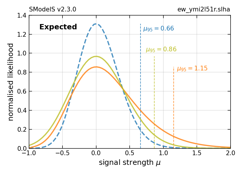
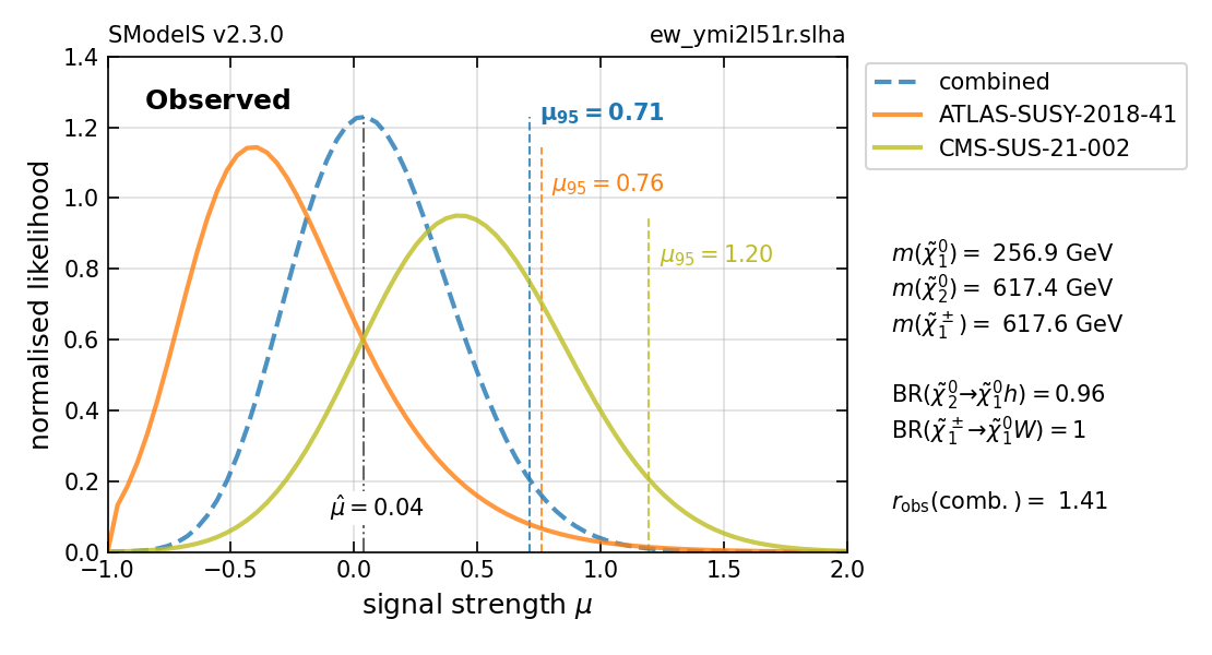
Figure 1: Visualisation of likelihoods for an EW-ino sample point with bino-like $\tilde{\chi}^{0}_{1}$ and wino-like $\tilde{\chi}^{\pm}_{1}$ and $\tilde{\chi}^{0}_{2}$ with masses $m_{\tilde{\chi}^{0}_{1}}=257$ GeV, $m_{\tilde{\chi}^{\pm}_{1},\tilde{\chi}^{0}_{2}}=617$ GeV. Shown are the expected likelihoods (left panel) and observed likelihoods (right panel) as a function of the signal strength $\mu$ for the two hadronic EW-ino searches from ATLAS and CMS and their combination.

With the observed data, however, shown in the plot on the right, the strongest constraint comes from the ATLAS-SUSY-2018-41 analysis, excluding the point with an $r_{\rm obs}=1.32$. The CMS-SUS-21-002 analysis only gives an $r_{\rm obs}$ value of $0.84$. The reason is that the former analysis observed a deficit of events, while the latter observed a small excess. In an analysis-by-analysis approach, one could exclude the point based on the highest observed $r$-value, or conclude that it is still allowed because the most sensitive analysis (the one with highest $r_{\rm exp}$) does not allow to exclude it. With the combined likelihood, however, one arrives at $r_{\rm obs}({\rm combined})=1.41$, thus robustly excluding the point.

We like to stress here that the expected limit always becomes stronger when combining. For the observed limit, however, the effect can go in either direction. The observed limit can become stronger, like in the example in Fig. 1. In the same way, it is possible that a point is excluded only by the combination of analyses, but not by any of the individual ones. But, the opposite can also happen, namely that a point excluded by some analysis becomes “unexcluded” by the combination with one or more other analyses. Indeed, all these cases will occur in the physics application in section 4.

An example code for visualising likelihoods and their combinations as in Fig. 1 is given in the How To’s section of the online manual. Moreover, there are code examples showing how to compute the confidence level of an exclusion, and how to define and use a “combinability matrix” that describes which analyses and/or SRs are approximately orthogonal and thus combinable.

3 Database update

The database update with respect to v2.1.0 [7] concerns the results from 9 ATLAS and 12 CMS publications. Concretely, the following results were added corresponding to the availability of appropriate public numerical material on HEPData:

Gluino/squark searches:

In this category, we added UL results from two CMS analyses, the search in final states with jets plus leptons CMS-SUS-19-008 [33] and the search in final states with jets plus highly boosted $Z$-bosons CMS-SUS-19-013 [34]. From ATLAS, we added the gluino/squark UL and EM results from the search in final states with jets plus two leptons, ATLAS-SUSY-2018-05 [35].

Stop/sbottom searches:

Here we added UL and EM results from two ATLAS publications: the stop search in the $2\ell$+jets channel, ATLAS-SUSY-2018-08 [36], and the sbottom search in final states with $b$-jets and taus (from $h\to\tau\tau$), ATLAS-SUSY-2018-40 [37]. On the CMS side, we added UL results from five publications, namely the $0\ell$ and $2\ell$ stop searches CMS-SUS-19-010 [38] and CMS-SUS-19-011 [39], the stop results from the search with soft leptons, CMS-SUS-18-004 [40], the sbottom results from CMS-SUS-18-007 [41], which uses $h\to\gamma\gamma$ decays, as well as the stop combination CMS-SUS-20-002 [42]. All these are results for full Run 2 luminosity: 139/fb for ATLAS and 137/fb for CMS. Moreover, lacking other EM results from CMS, we added the EMs which became available for CMS-SUS-16-050 [43], i.e. the $0\ell$ stop search for $35.9$/fb.

Electroweak searches:

These constitute the most important part of this database update. We added UL and EM results from ATLAS covering a large variety of EW-ino searches at Run 2; these are four searches in leptonic channels, ATLAS-SUSY-2018-05 (2 leptons) [35], ATLAS-SUSY-2018-32 (2 OS leptons) [29], ATLAS-SUSY-2019-02 (soft leptons) [44] and ATLAS-SUSY-2019-09 (3 leptons) [30], as well as the fully hadronic search ATLAS-SUSY-2018-41 [31]. For all these, the combination of SRs is enabled either through a HistFactory statistical model or a covariance matrix. It has to be stressed here that the HistFactory models provided by ATLAS are a real boon and enormously benefit reinterpretation studies! For the ATLAS-SUSY-2018-41 analysis, no HistFactory model is available so far, but ATLAS confirmed that the three SRs, for which EMs are available, are statistically independent, so we can trivially combine them assuming a diagonal covariance matrix. Last but not least, for completeness, we also added EM results for the search in final states with 3 leptons at 8 TeV, ATLAS-SUSY-2013-12 [45], which were previously missing and help cover low EW-ino masses. One analysis, which is not included although it does have extensive HEPData material, is the Run 2 search for electroweak production with compressed mass spectra ATLAS-SUSY-2018-16 [46]: the UL and EM results of this analysis depend on the assumed scenario, which conflicts with the default SModelS assumptions.

On the CMS side, the most important additions are the UL and EM results from the fully hadronic EW-ino search, CMS-SUS-21-002 [32], and the search for higgsinos decaying to Higgs bosons (with $h\to b\bar{b}$), CMS-SUS-20-004 [23]. Both analyses provide correlation and covariance matrices allowing for SRs combination. While the purely Gaussian SLv1 [9] works well for CMS-SUS-21-002, the CMS-SUS-20-004 analysis has highly asymmetric background uncertainties in several SRs, which makes the SLv1 a bad approximation of the full likelihood [22]. Thankfully, the background uncertainties are reported in non-symmetrised form in the paper [23], and we can use this information to compute the skew terms for the SLv2; CMS-SUS-20-004 is thus the first analysis in the SModelS database which uses the SLv2 following [18].

In addition to the above, we have implemented EW-ino UL results from CMS-SUS-18-007 [41], which is a search using Higgs boson to diphoton decays, and CMS-SUS-20-001 [47], a search for charginos and sleptons in final states with 2 leptons. It is deplorable, that other very relevant CMS analyses, like the EW-ino search in multi-lepton final states, CMS-SUS-19-012 (dedicated to Luc Pape!), and the search in $1\ell+h(\to b\bar{b})$ final states, CMS-SUS-20-003, provide no public material for reinterpretation or reuse.

Long-lived particles:

The previous database already contained a large number of results from searches for long-lived particles, as these had been the primary target of the v2.1.0 update [7]. In v2.3.0, one new analysis is added to this: the 139/fb ATLAS search for heavy, long-lived, charged particles with ${\rm d}E/{\rm d}x$ measurement, ATLAS-SUSY-2018-42 [48]. Concretely, we implemented the UL results for HSCPs (long-lived staus) and R-hadrons (long-lived gluinos) together with R-hadron EMs for the two inclusive SRs; the implementation of an EM binning in target mass is left for a future release. The analysis has also considered simplified models for long-lived charginos, but, unfortunately, the material provided for this is not sufficient for being used by SModelS [49].

Recast with MadAnalysis5:

In addition to the UL and EM results listed above, which were directly provided by ATLAS and CMS, we generated a number of “home-grown” EMs through recasting with MadAnalysis 5 [50, 51]. This helps fill gaps in EM coverage whenever a MadAnalysis 5 recast code is available. Concretely, we produced EMs for the $35.9$/fb leptonic EW-ino searches CMS-SUS-16-039 [52, 53] and CMS-SUS-16-048 [54, 55], and the $137$/fb multi-jet gluino and squark search CMS-SUS-19-006 [56, 57]. All three analyses come with a covariance matrix for SR combination in the SLv1 approach. The quality of the recasts is documented in [13].

With these additions, the SModelS v2.3.0 database now comprises results from 38 ATLAS and 40 CMS searches at Run 2 ($\sqrt{s}=13$ TeV), as well as 15 ATLAS and 18 CMS searches at Run 1 ($\sqrt{s}=8$ TeV), covering a total of 111 experimental publications. 17 of the ATLAS and 13 of the CMS searches are for full Run 2 luminosity. An overview of the complete database is given in Tables 1–3 in Appendix A and online at https://smodels.github.io/docs/ListOfAnalyses230. Validation plots for all results in the database are available online at https://smodels.github.io/docs/Validation230.

4 Physics impact

Since the largest part of the database update concerns searches for charginos and neutralinos, we demonstrate the physics impact of the new database and the new features in SModelS by means of constraints on the EW-ino sector of the MSSM. To this end, we reuse the EW-ino scan points from [7]. In section 4.2 of that paper, the relevant Lagrangian parameters, i.e. the bino and wino mass parameters $M_{1}$ and $M_{2}$, the higgsino mass parameter $\mu$, and $\tan\beta=v_{2}/v_{1}$ were randomly scanned over within the following ranges:

$$10\mbox{ GeV}< M_{1} <3\mbox{ TeV}\,,$$

$$100\mbox{ GeV}< M_{2} <3\mbox{ TeV}\,,$$

$$100\mbox{ GeV}< \mu <3\mbox{ TeV}\,,$$ (7)

$$5< \tan\beta <50\,.$$

The other SUSY breaking parameters were fixed to 10 TeV. The lower limits on $M_{2}$ and $\mu$ were chosen so as to avoid the LEP constraints on light charginos, and the lightest neutralino $\tilde{\chi}_{1}^{0}$ was required to be the lightest supersymmetric particle (LSP). The mass spectra and decay tables were computed with SoftSusy 4.1.11 [58, 59], which includes the $\tilde{\chi}^{\pm}_{1}\to\pi^{\pm}\tilde{\chi}^{0}_{1}$ decay calculation following [60] for small mass differences below about 1.5 GeV. Cross sections were computed first at leading order (LO) with Pythia 8 [61, 62], and reevaluated at next-to-LO with Prospino [63] for all points which had $r_{\rm max}\equiv\max(r_{\rm obs})>0.7$ in SModelS v2.1.0 with the LO cross sections.

From close to 100k points of the complete scan in [7], we here select the subset of points with only prompt decays (no long-lived particles, all decay widths $\Gamma_{\rm tot}>10^{-11}$ GeV). Moreover, we require $m_{\tilde{\chi}^{0}_{1}}<500$ GeV and $m_{\tilde{\chi}^{\pm}_{1}}<1200$ GeV in order to focus on the region which the current prompt EW-ino searches are sensitive to. This leaves us with 18544 points, which we analyse with SModelS v2.3.0.

The increase of exclusion power as compared to [7] is illustrated in Figure 2, which shows the number of excluded points as a function of the $\tilde{\chi}^{\pm}_{1}$ mass. The plot compares v2.1.0 to v2.3.0 with and without SR combination.  Different analyses are not combined at this stage. We note that the new experimental results in v2.3.0 extend the reach in chargino mass by about 300 GeV in the “best SR” approach (i.e., when SRs are not combined). Combination of SRs extends this reach by another 100 GeV, but mostly it increases the number of excluded points in the $m_{\tilde{\chi}^{\pm}_{1}}\approx 500$–1000 GeV mass range; this concerns primarily scenarios with a bino-like LSP. The effect comes mostly from the ATLAS-SUSY-2018-41 analysis, where the combination of SRs allows to simultaneously take into account the signal contributions to $VV$, $Vh$ and $hh$ final states ($V=W^{\pm},Z$), thus increasing the constraining power of the search. Finally, there is also a significant increase in the number of excluded points at low $m_{\tilde{\chi}^{\pm}_{1}}\lesssim 200$ GeV; these are to large extent points with a higgsino-like LSP. Overall, the number of excluded points increases from 661 with v2.1.0 to 2974 (1787) with v2.3.0 when SR combination is turned on (off).

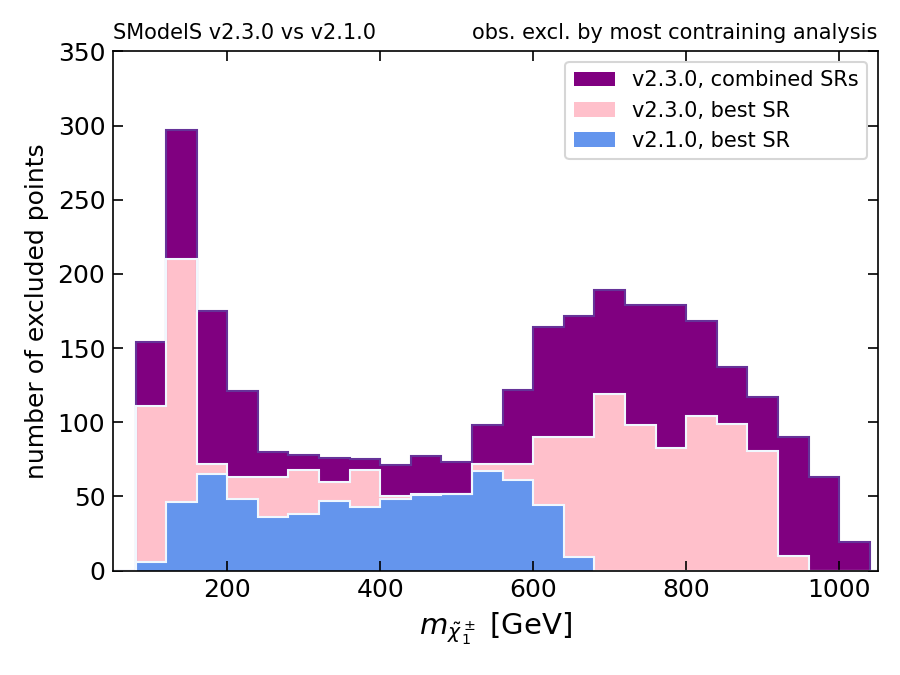
Figure 2: Comparison of exclusion power of SModelS v2.3.0 versus v2.1.0 as a function of the lighter chargino mass, $m_{\tilde{\chi}^{\pm}_{1}}$. Shown are the number of points excluded by the most constraining analysis, i.e. the number of points with $r_{\rm max}\equiv\max(r_{\rm obs})\geq 1$.

Given Figure 2, it is interesting to ask which experimental results are driving the exclusion in different regions of the parameter space. To answer this question, Figure 3 shows the points excluded by the LHC searches in the SModelS v2.3.0 database in the $m_{\tilde{\chi}_{1}^{\pm}}$ versus $m_{\tilde{\chi}_{1}^{0}}$ plane. The color of each excluded point denotes the most constraining analysis, that is the analysis giving the highest observed $r$-value. As can be seen, in the low mass range, $m_{\tilde{\chi}_{1}^{\pm}}\lesssim 500$ GeV, the constraints come from a variety of different analyses, while the high mass range, $m_{\tilde{\chi}_{1}^{\pm}}\gtrsim 500$ GeV is completely dominated by the ATLAS-SUSY-2018-41 analysis. The reason for this is that the ATLAS-SUSY-2018-41 analysis observed less events than expected (at least in the three super signal regions for which EMs are available) and therefore sets stronger limits than expected, and also stronger limits than the equivalent analysis from CMS, CMS-SUS-21-002, which saw a small excess in events.

This brings us to the issue that the most constraining analysis is not necessarily also the most sensitive one. From the statistics point of view, however, as long as limits are set on an analysis-by-analysis basis, using only the most sensitive result is the more rigorous approach in order to stay at the 95% confidence level. Indeed, as can be seen in Fig. 4, the picture changes quite significantly when considering the exclusion from the most sensitive analysis only. In particular when the most sensitive analysis is either the ATLAS or the CMS search in fully hadronic final states, the excluded region shrinks from $(m_{\tilde{\chi}^{\pm}_{1}},m_{\tilde{\chi}^{0}_{1}})\lesssim(1000,\,400)$ GeV in Fig. 3 to $(m_{\tilde{\chi}^{\pm}_{1}},m_{\tilde{\chi}^{0}_{1}})\lesssim(850,\,250)$ GeV in Fig. 4.

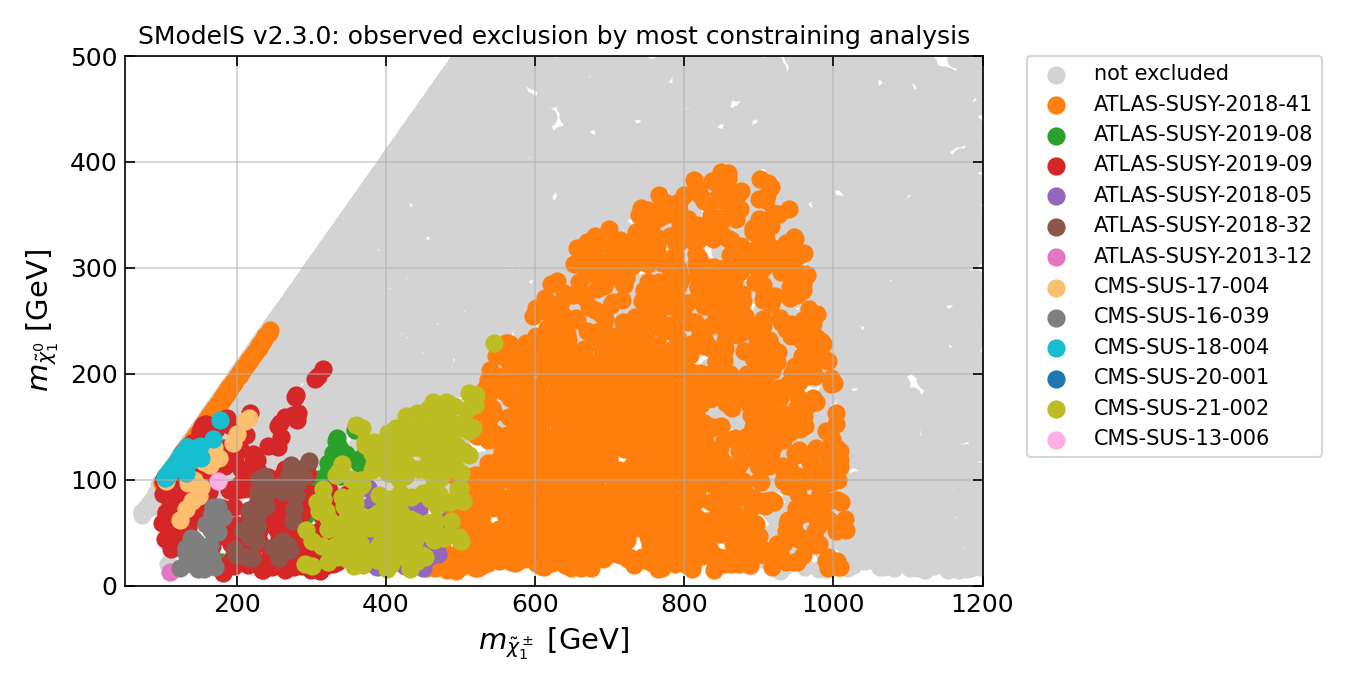
Figure 3: Scan points excluded by the most constraining analysis in SModelS v2.3.0, with combination of SRs turned on. The colour denotes the analysis that gives the highest $r$-value (see legend). Grey points are not excluded.

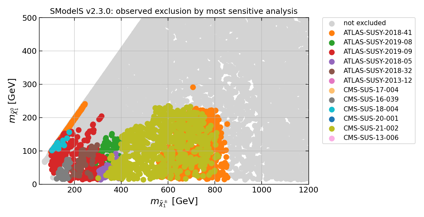
Figure 4: As Fig. 3 but for points excluded by the most sensitive analysis.

The assessment of the excluded parameter space can be improved by statistically combining the relevant analyses, as already demonstrated in Fig. 1 for a specific benchmark point. The results in Figs. 3 and 4 indeed motivate a combination of the two hadronic EW-ino searches, ATLAS-SUSY-2018-41 and CMS-SUS-21-002, as they are the most sensitive and/or most constraining ones in the high $m_{\tilde{\chi}^{\pm}_{1}}$ range (roughly for $m_{\tilde{\chi}^{\pm}_{1}}\gtrsim 400$ GeV). Figure 5 shows how the combination of these two analyses improves the sensitivity to EW-ino signals as compared to the single analysis approach: the expected limits are extended by about 200 GeV in chargino mass and by up to 100 GeV in LSP mass. The effect on the observed exclusion is shown Figure 6. Here, the khaki (light yellowish) and dark red coloured points are excluded by the combination, with the dark red points being those which are excluded only by the combination but not by either the ATLAS or the CMS analysis alone. In contrast, the light blue points would be excluded by one analysis, but are not excluded any more in the combination.

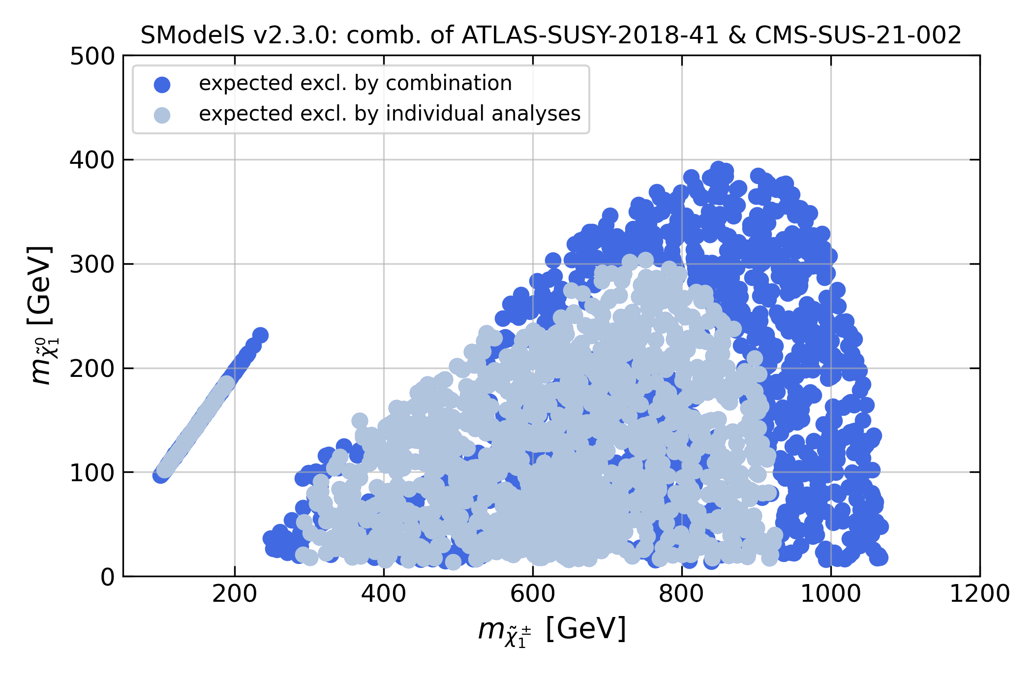
Figure 5: Effect of statistically combining the hadronic EW-ino searches from ATLAS and CMS, ATLAS-SUSY-2018-41 and CMS-SUS-21-002 on the expected reach: in light blue the expected exclusion of the individual ATLAS or CMS analyses, in dark blue the expected exclusion of the combination.

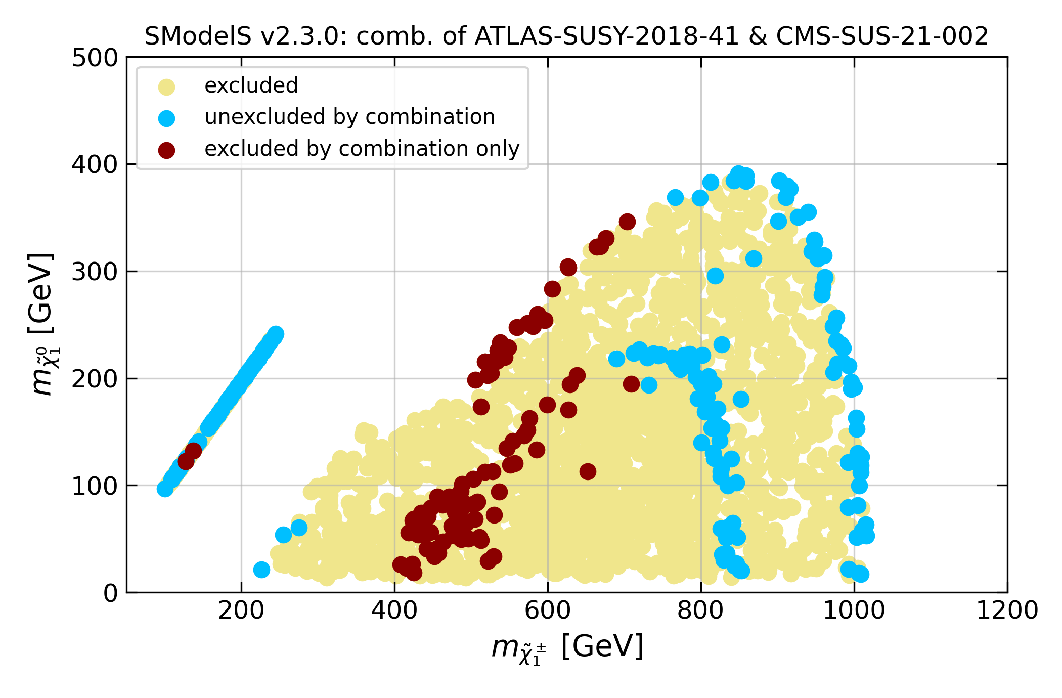
Figure 6: Effect of statistically combining the hadronic EW-ino searches from ATLAS and CMS, ATLAS-SUSY-2018-41 and CMS-SUS-21-002 on the observed limit. The khaki (light yellowish) and dark red coloured points are excluded at 95% confidence level by the combination, with the dark red points being those which are excluded only by the combination but not by one of the two analyses alone. The light blue points would be excluded by either ATLAS-SUSY-2018-41 or CMS-SUS-21-002, but are not excluded any more in the combination.

Concrete examples for a dark red and a light blue point from Fig. 6 are given in Figs. 7 and 8, respectively. The sample point in Fig. 7 lies at $(m_{\tilde{\chi}^{\pm}_{1}},m_{\tilde{\chi}^{0}_{1}})=(507,84)$ GeV, the point in Fig. 8 at $(m_{\tilde{\chi}^{\pm}_{1}},m_{\tilde{\chi}^{0}_{1}})=(834,36)$ GeV. Both feature a bino-like $\tilde{\chi}^{0}_{1}$ and higgsino-like $\tilde{\chi}^{\pm}_{1}$, $\tilde{\chi}^{0}_{2,3}$. Moreover, in both cases neither the ATLAS nor the CMS hadronic analysis is expected to exclude the point; only the combination of both analyses gives high enough sensitivity. For the point in Fig. 7, this behaviour is replicated also with the observed data: indeed we find $r_{\rm obs}=0.81$ and $0.93$ for the CMS and ATLAS analysis, respectively, so neither analysis individually excludes the point (recall that $r=1/\mu_{95}$). In the combination, this moves to $r_{\rm obs}({\rm comb.})=1.22$, resulting in a solid exclusion. In contrast, in the example in Fig. 8, the behaviour of the observed limits is quite different: the ATLAS analysis excludes the point with an $r_{\rm obs}$ of $1.07$, while the CMS analysis, although having very similar sensitivity, gives only $r_{\rm obs}=0.39$. Combining the two analyses results in $r_{\rm obs}({\rm comb.})=0.95$, which means the point is not excluded any more.

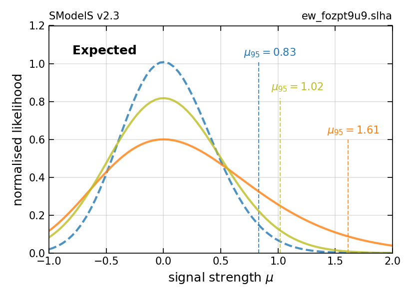
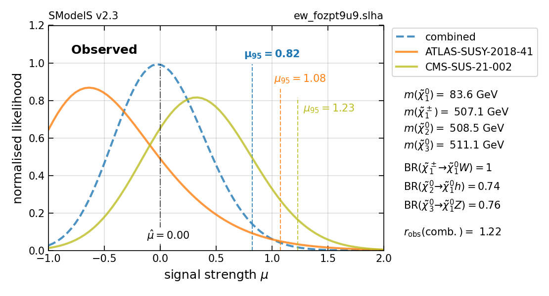
Figure 7: Visualisation of likelihoods for one of the dark red points from Fig. 6, i.e. a point which is only excluded by the combination of the considered ATLAS and CMS analyses, but not by any of the two analyses alone. See text for details.

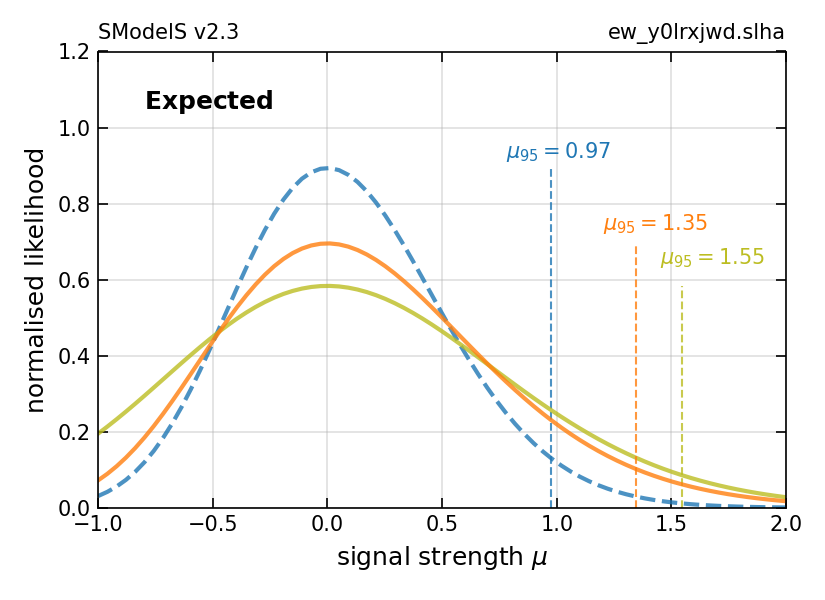
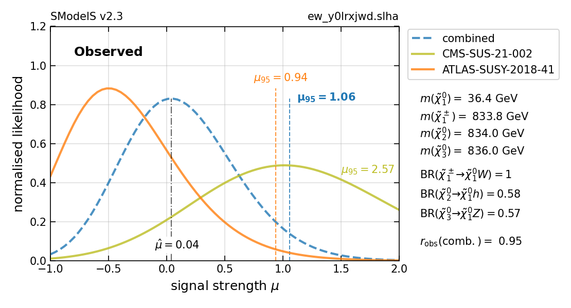
Figure 8: Visualisation of likelihoods for one of the light blue points from Fig. 6, concretely a point which is excluded by the ATLAS analysis, but not any more so when combining it with the CMS analysis. See text for details.

Altogether, the combination of the ATLAS and CMS hadronic EW-ino searches excludes 2258 of the scan points. Of the remaining points, further 614 are excluded by some other EW-ino search. This gives a total of 2872 excluded points, as compared to 2974 (2048) when considering the limit from the most constraining (most sensitive) analysis only. Indeed the overall change in the observed limit when comparing Fig. 6 to Fig. 3 is rather small. This is due to the data under-fluctuations (with respect to the expected background) seen by the hadronic ATLAS search and the over-fluctuations seen by the CMS one. The combined limit is, however, statistically more reliable, since it makes use of a larger amount of data coming from both the ATLAS and CMS searches.

A comment is in order regarding the bino, wino and higgsino mixing. The bulk of the excluded points at $m_{\tilde{\chi}^{\pm}_{1}}\approx 200$–$1000$ GeV in Fig. 6 has a (mostly) bino-like LSP, with the next heavier states being mostly higgsino- or wino-like; highly mixed charginos and neutralinos make only a fraction of the scan points, due to volume effects. As a consequence, the dark red and light blue points form two “arcs” in the $m_{\tilde{\chi}_{1}^{\pm}}$ versus $m_{\tilde{\chi}_{1}^{0}}$ plane, the lower one featuring higgsino-like $\tilde{\chi}_{1}^{\pm}$ and $\tilde{\chi}^{0}_{2,3}$ and the higher one featuring wino-like $\tilde{\chi}_{1}^{\pm}$ and $\tilde{\chi}^{0}_{2}$. The few dark red/light blue points scattered away from these arcs have significant wino-higgsino mixing. The isolated diagonal line of points at $m_{\tilde{\chi}^{\pm}_{1}}\approx 100$–$250$ GeV, on the other hand, is characterised by a higgsino-like LSP, with the signal coming from the production of wino-like $\tilde{\chi}_{2}^{\pm}$ and $\tilde{\chi}^{0}_{3}$. In Appendix D we provide auxiliary results in terms of the relevant MSSM parameters, which illustrate the above statements.

All in all, the combination of analyses, here illustrated by the example of combining the fully hadronic EW-ino searches from ATLAS and CMS, leads to better and statistically more robust constraints: first, combinations of analyses use more of the available data thus increasing the sensitivity to the BSM signal; second, while individual analyses can lead to an over(under)-aggressive exclusion of the parameter space due to under(over)-fluctuations of the data with respect to the expected background, the combination of analyses reduces the impact of such fluctuations.

5 Conclusions

The wealth of experimental constraints on new physics from Run 2 of the LHC makes it increasingly important to be able to perform global (re)interpretation studies. The aim is to find out on the one hand how all the available experimental information constrains complicated scenarios, and on the other hand what are the most likely regions where new physics can still manifest itself at the LHC. This requires software tools that encompass searches in as many final states as possible, and that can build global likelihoods from them.

The SModelS package is a public tool that can be useful in this endeavour. It is designed for the fast reinterpretation of LHC searches for new physics on the basis of simplified-model results, mostly stemming from searches for supersymmetric particles. Owing to its speed, it is particularly well suited for large scans and model surveys.

Version 2.3 of SModelS, presented in this paper, comes with a significant database update with the latest available experimental results for full Run 2 luminosity. In total, the SModelS database now comprises results from 38 ATLAS and 40 CMS searches at Run 2, as well as 15 ATLAS and 18 CMS searches at Run 1, covering a total of 111 experimental publications. 17 of the ATLAS and 13 of the CMS searches are for full Run 2 luminosity. This comprises in particular the full suit of available and reusable electroweak-ino searches from Run 2.

On the code side, the most important new feature is the ability to combine likelihoods from different analyses. This enables statistically more rigorous constraints and opens the way for global likelihood analyses for LHC searches. We reviewed the different ways of computing likelihoods for a signal hypothesis from the publicly available information, and explained how likelihoods can be combined in SModelS.

The physics impact was demonstrated by means of a case study of the electroweak-ino sector of the MSSM. With the new database, the reach in chargino mass increases from about 650 GeV in [7] to about 1 TeV in v2.3.0. for promptly decaying EW-inos. The total number of excluded points increases by more than a factor of four with respect to [7]. Last but not least, we exemplified how the combination of approximately independent analyses helps average out statistical fluctuations and thus leads to more robust limits. An extensive global study of the EW-ino sector of the MSSM is in preparation.

Data management:

SModelS is public software distributed under the GNU General Public License v3 (GPLv3). It is available on GitHub and in the Python Package Index (PyPI). The SModelS database is available in text form on GitHub and as a binary pickle file on Zenodo [64]. The complete dataset (input and output files) from the EW-ino scan used in this paper is also made available on Zenodo [65], ensuring full reproducibility of the results presented in this paper.

Appendix A Complete list of experimental results in the v2.3.0 database

ID	Short Description	$\mathcal{L}$ [fb-1]	ULobs	ULexp	EM	comb.
ATLAS-SUSY-2015-01 [66]	2 $b$-jets	3.2
ATLAS-SUSY-2015-02 [67]	$1\ell$ stop	3.2
ATLAS-SUSY-2015-06 [68]	$0\ell$ + 2–6 jets	3.2
ATLAS-SUSY-2015-09 [69]	jets + 2 SS or $\geq 3\ell$	3.2
ATLAS-SUSY-2016-06 [70]	disappearing tracks	36.1
ATLAS-SUSY-2016-07 [71]	$0\ell$ + jets	36.1
ATLAS-SUSY-2016-08 [72]	displaced vertices	32.8
ATLAS-SUSY-2016-14 [73]	2 SS or 3 $\ell$’s + jets	36.1
ATLAS-SUSY-2016-15 [74]	$0\ell$ stop	36.1
ATLAS-SUSY-2016-16 [75]	$1\ell$ stop	36.1
ATLAS-SUSY-2016-17 [76]	2 OS $\ell$	36.1
ATLAS-SUSY-2016-19 [77]	2 $b$-jets + $\tau$’s	36.1
ATLAS-SUSY-2016-24 [78]	2–3 $\ell$’s, EWK	36.1
ATLAS-SUSY-2016-26 [79]	$\geq 2\,c$-jets	36.1
ATLAS-SUSY-2016-27 [80]	jets + $\gamma$	36.1
ATLAS-SUSY-2016-28 [81]	2 $b$-jets	36.1
ATLAS-SUSY-2016-32 [82]	HSCP	31.6
ATLAS-SUSY-2016-33 [83]	2 SFOS $\ell$’s	36.1
ATLAS-SUSY-2017-01 [84]	$Wh(bb)$, EWK	36.1
ATLAS-SUSY-2017-02 [85]	$0\ell$ + jets	36.1
ATLAS-SUSY-2017-03 [86]	multi-$\ell$ EWK	36.1
ATLAS-SUSY-2018-04 [87]	2 hadronic taus	139.0				Pyhf
ATLAS-SUSY-2018-05 [35]	$2\ell$ + jets, EWK	139.0				Pyhf
ATLAS-SUSY-2018-05 [35]	$2\ell$ + jets, strong	139.0
ATLAS-SUSY-2018-06 [88]	$3\ell$, EWK	139.0
ATLAS-SUSY-2018-08 [36]	2 OS $\ell$	139.0
ATLAS-SUSY-2018-10 [89]	1$\ell$ + jets	139.0
ATLAS-SUSY-2018-12 [90]	0$\ell$ + jets	139.0
ATLAS-SUSY-2018-14 [91]	displaced vertices	139.0				Pyhf
ATLAS-SUSY-2018-22 [92]	multi-jets	139.0
ATLAS-SUSY-2018-23 [93]	$Wh(\gamma\gamma)$, EWK	139.0
ATLAS-SUSY-2018-31 [94]	2$b$ + 2$h(bb)$	139.0				Pyhf
ATLAS-SUSY-2018-32 [29]	2 OS $\ell$	139.0				Pyhf
ATLAS-SUSY-2018-40 [37]	2$b$ + 2$h(\tau\tau)$	139.0
ATLAS-SUSY-2018-41 [31]	hadr. EWK search	139.0				SLv1
ATLAS-SUSY-2018-42 [48]	charged LLPs, dE/dx	139.0
ATLAS-SUSY-2019-02 [44]	2 soft $\ell$’s, EWK	139.0				SLv1
ATLAS-SUSY-2019-08 [28]	1$\ell$ + $h(bb)$, EWK	139.0				Pyhf
ATLAS-SUSY-2019-09 [30]	$3\ell$, EWK	139.0				Pyhf

Table 1: List of ATLAS Run 2 analyses and their types of results in the SModelS v2.3.0 database. Apart from the HSCP, disappearing tracks and displaced lepton searches, all analyses require ${\not{E}_{T}}$ in the final state (for conciseness omitted in the short descriptions). EWK stands for electroweak (-ino or slepton) production. The last column specifies whether and how SRs are combined. New additions are highlighted in bold.

ID	Short Description	$\mathcal{L}$ [fb-1]	ULobs	ULexp	EM	comb.
CMS-PAS-EXO-16-036 [95]	HSCP	12.9
CMS-PAS-SUS-16-052 [96]	ISR jet + soft $\ell$	35.9				SLv1
CMS-SUS-16-009 [97]	$0\ell$ + jets, top tag	2.3
CMS-SUS-16-032 [98]	2 $b$- or 2 $c$-jets	35.9
CMS-SUS-16-033 [99]	0$\ell$ + jets	35.9
CMS-SUS-16-034 [100]	2 SFOS $\ell$	35.9
CMS-SUS-16-035 [101]	2 SS $\ell$	35.9
CMS-SUS-16-036 [102]	0$\ell$ + jets	35.9
CMS-SUS-16-037 [103]	1$\ell$ + jets with MJ	35.9
CMS-SUS-16-039 [52]	multi-$\ell$, EWK	35.9				SLv1
CMS-SUS-16-041 [104]	multi-$\ell$ + jets	35.9
CMS-SUS-16-042 [105]	1$\ell$ + jets	35.9
CMS-SUS-16-043 [106]	$Wh(bb)$, EWK	35.9
CMS-SUS-16-045 [107]	2 $b$ + 2 $h(\gamma\gamma)$	35.9
CMS-SUS-16-046 [108]	high-$p_{T}$ $\gamma$	35.9
CMS-SUS-16-047 [109]	$\gamma$ + jets, high $H_{T}$	35.9
CMS-SUS-16-048 [54]	2 OS $\ell$, soft	35.9				SLv1
CMS-SUS-16-050 [43]	0$\ell$ + top tag	35.9				SLv1
CMS-SUS-16-051 [110]	1$\ell$ stop	35.9
CMS-SUS-17-003 [111]	2 taus	35.9
CMS-SUS-17-004 [112]	EWK combination	35.9
CMS-SUS-17-005 [113]	1$\ell$ + jets, top tag	35.9
CMS-SUS-17-006 [114]	jets + boosted $h(bb)$	35.9
CMS-SUS-17-009 [115]	SFOS $\ell$	35.9
CMS-SUS-17-010 [116]	2$\ell$ stop	35.9
CMS-SUS-18-002 [117]	$\gamma$ + ($b$-)jets, top tag	35.9
CMS-SUS-18-004 [40]	2–3 soft $\ell$’s	137.0
CMS-SUS-18-007 [41]	$2\,h(\gamma\gamma)$, EWK	77.5
CMS-EXO-19-001 [118]	non-prompt jets	137.0
CMS-EXO-19-010 [119]	disappearing tracks	101.0
CMS-SUS-19-006 [56]	0$\ell$ + jets, MHT	137.0				SLv1
CMS-SUS-19-008 [33]	2–3$\ell$ + jets	137.0
CMS-SUS-19-009 [120]	1$\ell$ + jets, MHT	137.0
CMS-SUS-19-010 [38]	jets + top and $W$-tag	137.0
CMS-SUS-19-011 [39]	$2\ell$ stop	137.0
CMS-SUS-19-013 [34]	jets + boosted $Z$’s	137.0
CMS-SUS-20-001 [47]	SFOS $\ell$	137.0
CMS-SUS-20-002 [42]	stop combination	137.0
CMS-SUS-20-004 [23]	2 $h(bb)$, EWK	137.0				SLv2
CMS-SUS-21-002 [32]	hadr. EWK search	137.0				SLv1

Table 2: List of CMS Run 2 analyses and their types of results in the SModelS v2.3.0 database. Apart from the HSCP, disappearing tracks and displaced lepton searches, all analyses require ${\not{E}_{T}}$ in the final state (for conciseness omitted in the short descriptions). EWK stands for electroweak (-ino or slepton) production. The last column specifies whether and how SRs are combined. New additions are highlighted in bold.

ID	Short Description	$\mathcal{L}$ [fb-1]	ULobs	ULexp	EM
ATLAS-SUSY-2013-02 [121]	0$\ell$ + 2–6 jets	20.3
ATLAS-SUSY-2013-04 [122]	0$\ell$ + 7–10 jets	20.3
ATLAS-SUSY-2013-05 [123]	0$\ell$ + 2$b$-jets	20.1
ATLAS-SUSY-2013-08 [124]	$Z(\ell\ell)$ + $b$-jets	20.3
ATLAS-SUSY-2013-09 [125]	2 SS $\ell$ + 0–3 $b$-jets	20.3
ATLAS-SUSY-2013-11 [126]	2$\ell$ ($e,\mu$), EWK	20.3
ATLAS-SUSY-2013-12 [45]	3$\ell$ ($e,\mu,\tau$), EWK	20.3
ATLAS-SUSY-2013-15 [127]	1$\ell$ + 4 (1$b$) jets	20.3
ATLAS-SUSY-2013-16 [128]	0$\ell$ + 6 (2$b$) jets	20.1
ATLAS-SUSY-2013-18 [129]	jets + $\geq 3b$-jets	20.1
ATLAS-SUSY-2013-19 [130]	2 OS $\ell$ + ($b$-)jets	20.3
ATLAS-SUSY-2013-20 [131]	2$\ell$ ($e,\mu$) + jets	20.3
ATLAS-SUSY-2013-21 [132]	monojet or $c$-jet	20.3
ATLAS-SUSY-2013-23 [133]	1$\ell$ + 2 $b$-jets (or 2$\gamma$)	20.3
ATLAS-SUSY-2014-03 [134]	$\geq 2$ ($c$-)jets	20.3
CMS-EXO-12-026 [135]	HSCP	18.8
CMS-EXO-13-006 [136]	HSCP	18.8
CMS-PAS-SUS-13-015 [137]	$\geq 5$ ($1b$) jets	19.4
CMS-PAS-SUS-13-016 [138]	2$\ell$ + $\geq 4$ ($2b$) jets	19.7
CMS-PAS-SUS-13-018 [139]	1–2 $b$-jets, $M_{\rm CT}$	19.4
CMS-PAS-SUS-13-023 [140]	$0\ell$ stop	18.9
CMS-SUS-12-024 [141]	0$\ell$ + $\geq 3$ ($1b$) jets	19.4
CMS-SUS-12-028 [142]	multi ($b$-)jets, $\alpha_{T}$	11.7
CMS-SUS-13-002 [143]	$\geq 3\ell$ (+jets)	19.5
CMS-SUS-13-004 [144]	$\geq 1b$-jet, Razor	19.3
CMS-SUS-13-006 [145]	multi-$\ell$, EWK	19.5
CMS-SUS-13-007 [146]	1$\ell$ + $\geq 2b$-jets	19.3
CMS-SUS-13-011 [147]	1$\ell$ + $\geq 4$ ($1b$)jets	19.5
CMS-SUS-13-012 [148]	jets + $\not\!\!H_{T}$	19.5
CMS-SUS-13-013 [149]	2 SS $\ell$ + ($b$-)jets	19.5
CMS-SUS-13-019 [150]	$\geq 2$ jets, $M_{\rm T2}$	19.5
CMS-SUS-14-010 [151]	$b$-jets + 4$W$	19.5
CMS-SUS-14-021 [152]	soft $\ell$, low jet mult.	19.7

Table 3: List of 15 ATLAS and 18 CMS Run 1 analyses and their types of results in the SModelS v2.3.0 database. Apart from the HSCP searches, all analyses require ${\not{E}_{T}}$ in the final state (for conciseness omitted in the short descriptions). EWK stands for electroweak(-ino) production. New in v2.3.0 are the EMs for ATLAS-SUSY-2013-12. The column comb. from Tables 1–2 is omitted because none of the Run 1 analyses provides any information on background correlations.

Appendix B Database add-ons

When running SModelS, the user has to specify which database to use. This is done in the parameters.ini file by giving the path to the smodels-database folder, the path to a pickle file or a URL path. Details are explained in the Using SModelS section of the online manual. The available databases can be seen on the smodels-database-release page on github.

Shorthand notations are available: path=official refers to the official database of the users’ SModelS version, while path=latest refers to the latest available database release. The ‘+’ operator allows for extending the “official” or “latest” database with add-ons:

+fastlim:

adds fastlim results (from early 8 TeV ATLAS analyses); from v2.1.0 onward

+superseded:

adds results which were previously available but were superseded by newer ones; from v2.1.0 onward

+nonaggregated:

adds analyses with non-aggregated SRs in addition to the aggregated results in CMS analyses; from v2.2.0 onward

+full_llhds:

replaces simplified HistFactory statistical models by full ones in ATLAS analyses; from v2.3.0 onward (careful, this increases a lot the runtime!)

Examples are “official+nonaggregated” or “official+nonaggregated+full_llhds”. Note that order matters: results are replaced in the specified sequence, so “full_llhds+official” will fall back onto the official database with simplified HistFactory statistical models. The add-ons can also be used alone, e.g. path=full_llhds, though this is of limited practical use. Finally, “debug” refers to a version of the database with extra information that is however not intended for usage by a regular user and only mentioned here for completeness.

Appendix C Examples combining more than two analyses

The benchmark point used in Fig. 1 is in fact constrained not only by the two hadronic EW-ino searches ATLAS-SUSY-2018-41 [31] and CMS-SUS-21-002 [32], but also by the search for $\tilde{\chi}^{\pm}_{1}\tilde{\chi}^{0}_{2}\to Wh+{\not{E}_{T}}$ in the $1\ell+b\bar{b}+{\not{E}_{T}}$ final state, ATLAS-SUSY-2019-08 [28] (other analyses in the SModelS database do not give any relevant constraints). Assuming that hadronic searches (vetoing leptons) and leptonic ones (requiring leptons) are independent to good approximation, we can combine all three analyses. The result is shown in Fig. 9. The combined sensitivity increases to $r_{\rm exp}=1.67$, while the observed $r$-value moves to $r_{\rm obs}=1.32$, compared to $r_{\rm exp}=1.52$ and $r_{\rm obs}=1.41$ in Fig. 1.

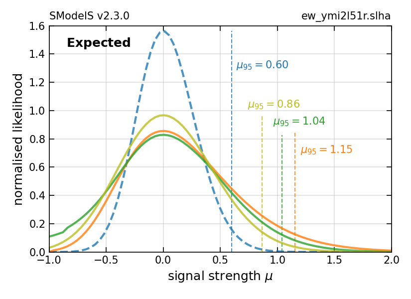
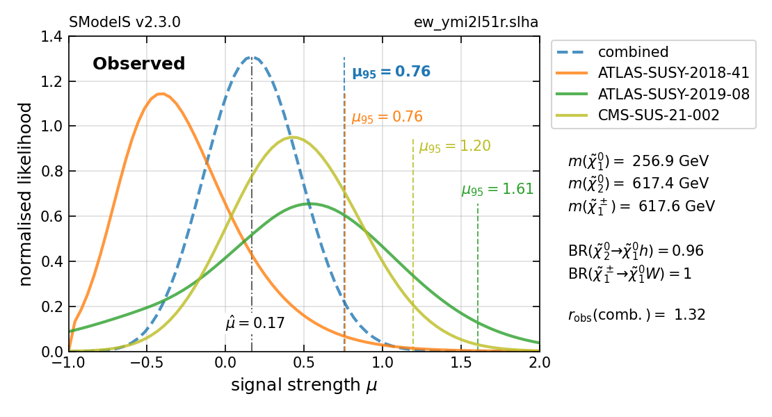
Figure 9: Same as Fig. 1 but including also the ATLAS-SUSY-2019-08 analysis ($1\ell+b\bar{b}+{\not{E}_{T}}$ final state) in the combination. The combined sensitivity increases to $r_{\rm exp}=1.67$, while the observed $r$-value moves to $r_{\rm obs}=1.32$ (compared to $r_{\rm exp}=1.52$ and $r_{\rm obs}=1.41$ in Fig. 1).

Figure 10 shows an EW-ino scenario with a bino-like $\tilde{\chi}^{0}_{1}$ with mass around 140 GeV, and higgsino-like $\tilde{\chi}^{0}_{2,3},\tilde{\chi}^{\pm}_{1}$ with masses around $555$ GeV; the wino-like states have masses of $2.3$ TeV. This scenario is not excluded by any of the individual analyses in the SModelS v2.3.0 database. Concretely, we get the following results:

Analysis	final state	$r_{\rm exp}$	$r_{\rm obs}$
CMS-SUS-21-002	hadronic	0.81	0.63
ATLAS-SUSY-2018-41	hadronic	0.63	0.92
ATLAS-SUSY-2018-05	$2\ell$ + jets	0.46	0.68
ATLAS-SUSY-2019-08	$1\ell+b\bar{b}$	0.42	0.27

Again, the highest sensitivity comes from the hadronic EW-ino searches ATLAS-SUSY-2018-41 and CMS-SUS-21-002, and combining them one reaches $r_{\rm exp}=1.06$ and $r_{\rm obs}=1.05$. In Fig. 6 in section 4, the point thus appears as newly excluded by the combination. Nonetheless the other two ATLAS analyses are not irrelevant: including them in the combination, the sensitivity increases to $r_{\rm exp}=1.30$, and the observed exclusion increases to $r_{\rm obs}=1.34$, see Fig. 10. It is interesting to note how the deficits of events in ATLAS-SUSY-2018-41 and ATLAS-SUSY-2018-05 on the one hand, and the small excesses of events in CMS-SUS-21-002 and ATLAS-SUSY-2019-08 on the other hand are averaged out so that in the end $r_{\rm obs}\approx r_{\rm exp}$ in the combination.

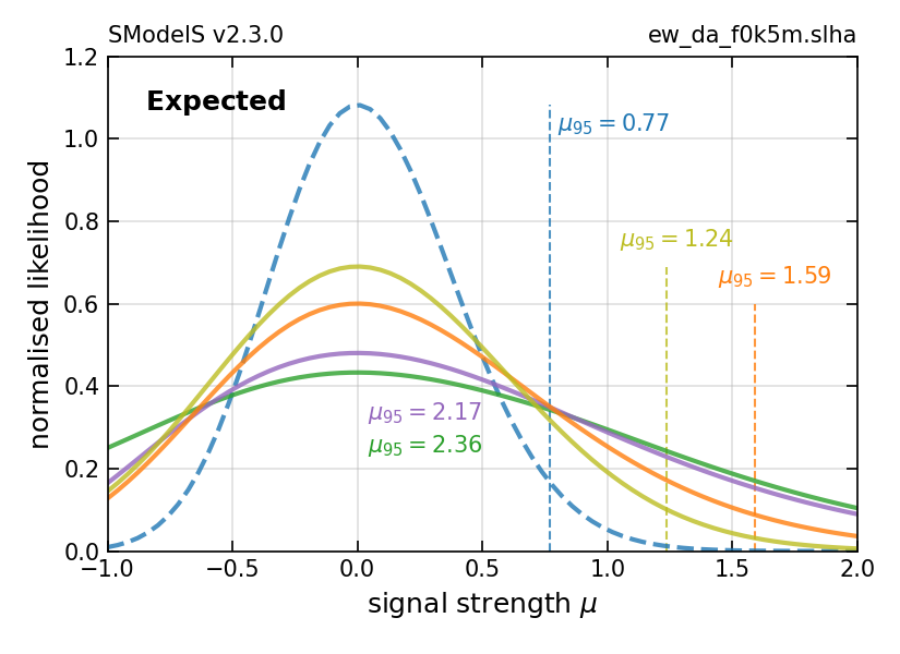
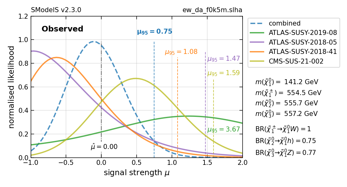
Figure 10: Visualisation of likelihoods for an EW-ino sample point with bino-like $\tilde{\chi}^{0}_{1}$ and higgsino-like $\tilde{\chi}^{\pm}_{1}$, $\tilde{\chi}^{0}_{2,3}$ with masses $m_{\tilde{\chi}^{0}_{1}}=141$ GeV, $m_{\tilde{\chi}^{\pm}_{1},\tilde{\chi}^{0}_{2,3}}\approx 555$ GeV. See text for details.

Appendix D Auxiliary plots supplementing the results of section 4

In this Appendix we present a number of additional plots which may be of interest to the reader. In particular, these are projections of the results from section 4 in terms of the gaugino and higgsino mass parameters $M_{1}$, $M_{2}$ and $\mu$, giving more insights into the mass hierarchies and mixings at play.

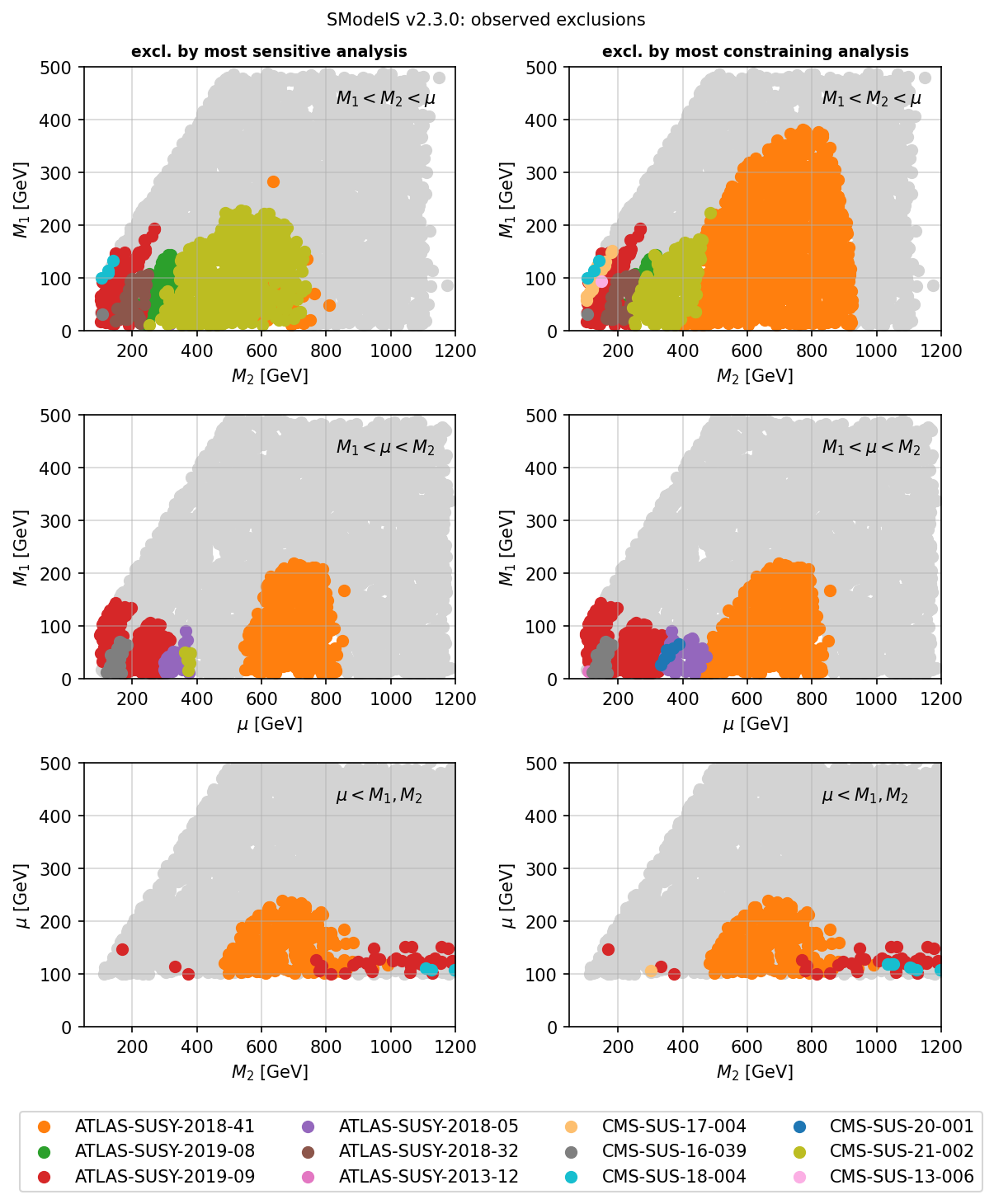
Figure 11: Scan points excluded by the most sensitive analysis (left panels) or the most constraining analysis (right panels) in terms of $M_{1}$, $M_{2}$ and $\mu$. Three different hierarchies are considered: $M_{1}<M_{2}<\mu$ (top row), $M_{1}<\mu<M_{2}$ (middle row) and $\mu<M_{1},\,M_{2}$ (bottom row).

Figure 11 shows the scan points excluded by the most sensitive or the most constraining analysis, equivalent to Figs. 3 and 4 in section 4. The three cases considered are:
– top row: $M_{1}<M_{2}<\mu$, leading to a bino-like $\tilde{\chi}^{0}_{1}$ and wino-like $\tilde{\chi}^{0}_{2}$ and $\tilde{\chi}^{\pm}_{1}$;
– middle row: $M_{1}<\mu<M_{2}$, leading to a bino-like $\tilde{\chi}^{0}_{1}$, higgsino-like $\tilde{\chi}^{0}_{2,3}$ and $\tilde{\chi}^{\pm}_{1}$; and
– bottom row: $\mu<M_{1},\,M_{2}$, leading to higgsino-like and near mass-degenerate $\tilde{\chi}^{0}_{1,2}$ and $\tilde{\chi}^{\pm}_{1}$.

The gaugino/higgsino mixing is further illustrated in Fig. 12, which shows the scan points excluded by the most constraining analysis in the plane of $M_{2}/M_{1}$ versus $M_{2}/\mu$. The points below the dashed line are in the compressed region ($m_{\tilde{\chi}^{\pm}_{1}}-m_{\tilde{\chi}^{0}_{1}}<10$ GeV) and correspond to the higgsino LSP scenario. Note that the wino-LSP scenario ($M_{2}<M_{1},\mu$) is not considered, since it leads to long-lived charginos.

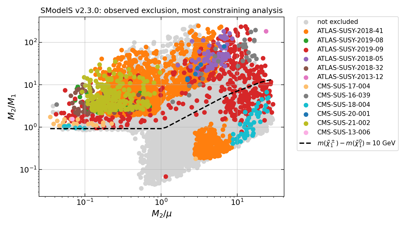
Figure 12: Scan points excluded by the most constraining analysis in the plane of $M_{2}/M_{1}$ versus $M_{2}/\mu$.

Last but not least, as a supplement to Figs. 5 and 6, Fig. 13 shows the expected and observed exclusion obtained from the combination of the ATLAS and CMS hadronic EW-ino searches in the $M_{1}$ vs. $M_{2}$, $M_{1}$ vs. $\mu$ and $\mu$ vs. $M_{2}$ planes for the same three cases as above (top left, top right and bottom left panels, respectively). The forth panel on the bottom right shows the projection of the excluded points onto the $M_{2}/M_{1}$ versus $M_{2}/\mu$ plane.

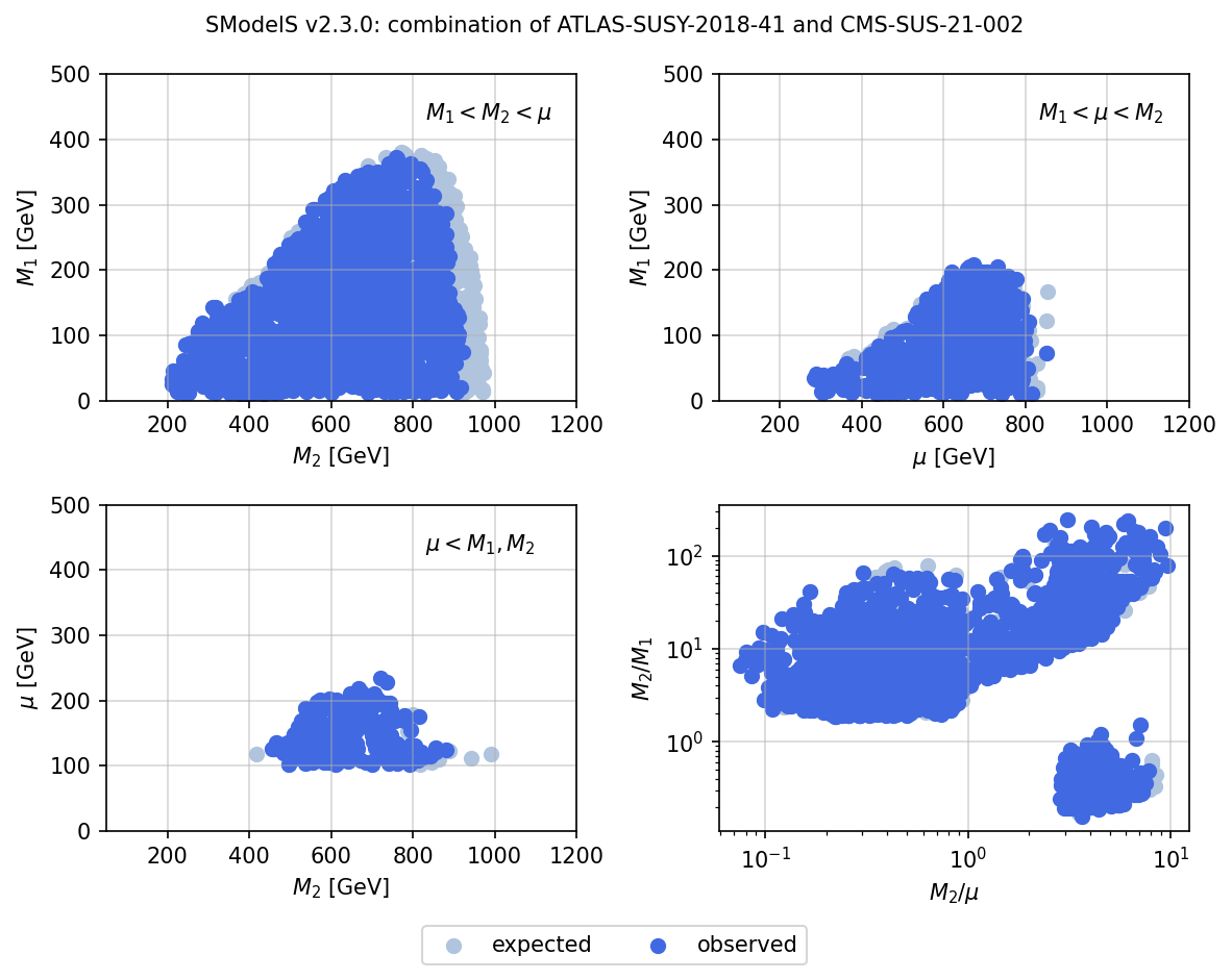
Figure 13: Expected and observed exclusion by the combination of the ATLAS and CMS hadronic EW-ino searches in terms of $M_{1}$, $M_{2}$ and $\mu$. Note that, except for a small strip at high $M_{2}$, the expected and observed exclusions are almost the same.

References

- [1] S. Kraml et al., Searches for New Physics: Les Houches Recommendations for the Presentation of LHC Results, Eur. Phys. J. C 72, 1976 (2012), 10.1140/epjc/s10052-012-1976-3, arXiv:1203.2489.
- [2] W. Abdallah et al., Reinterpretation of LHC Results for New Physics: Status and Recommendations after Run 2, SciPost Phys. 9(2), 022 (2020), 10.21468/SciPostPhys.9.2.022, arXiv:2003.07868.
- [3] S. Bailey et al., Data and Analysis Preservation, Recasting, and Reinterpretation (2022), whitepaper submitted to Snowmass 2021, arXiv:2203.10057.
- [4] S. Kraml, S. Kulkarni, U. Laa, A. Lessa, W. Magerl, D. Proschofsky-Spindler and W. Waltenberger, SModelS: a tool for interpreting simplified-model results from the LHC and its application to supersymmetry, Eur. Phys. J. C 74, 2868 (2014), 10.1140/epjc/s10052-014-2868-5, arXiv:1312.4175.
- [5] F. Ambrogi, S. Kraml, S. Kulkarni, U. Laa, A. Lessa, V. Magerl, J. Sonneveld, M. Traub and W. Waltenberger, SModelS v1.1 user manual: Improving simplified model constraints with efficiency maps, Comput. Phys. Commun. 227, 72 (2018), 10.1016/j.cpc.2018.02.007, arXiv:1701.06586.
- [6] F. Ambrogi et al., SModelS v1.2: long-lived particles, combination of signal regions, and other novelties, Comput. Phys. Commun. 251, 106848 (2020), 10.1016/j.cpc.2019.07.013, arXiv:1811.10624.
- [7] G. Alguero, J. Heisig, C. K. Khosa, S. Kraml, S. Kulkarni, A. Lessa, H. Reyes-González, W. Waltenberger and A. Wongel, Constraining new physics with SModelS version 2, JHEP 08, 068 (2022), 10.1007/JHEP08(2022)068, arXiv:2112.00769.
- [8] K. Cranmer et al., Publishing statistical models: Getting the most out of particle physics experiments, SciPost Phys. 12(1), 037 (2022), 10.21468/SciPostPhys.12.1.037, arXiv:2109.04981.
- [9] CMS Collaboration, Simplified likelihood for the re-interpretation of public CMS results, Tech. Rep. CMS-NOTE-2017-001, CERN, Geneva (2017).
- [10] ATLAS Collaboration, Reproducing searches for new physics with the ATLAS experiment through publication of full statistical likelihoods, Tech. Rep. ATL-PHYS-PUB-2019-029, CERN, Geneva (2019).
- [11] P. Athron et al., Combined collider constraints on neutralinos and charginos, Eur. Phys. J. C 79(5), 395 (2019), 10.1140/epjc/s10052-019-6837-x, arXiv:1809.02097.
- [12] G. Alguero, S. Kraml and W. Waltenberger, A SModelS interface for pyhf likelihoods, Comput. Phys. Commun. 264, 107909 (2021), 10.1016/j.cpc.2021.107909, arXiv:2009.01809.
- [13] G. Alguero, J. Y. Araz, B. Fuks and S. Kraml, Signal region combination with full and simplified likelihoods in MadAnalysis 5, SciPost Phys. 14(1), 009 (2023), 10.21468/SciPostPhys.14.1.009, arXiv:2206.14870.
- [14] V. Ananyev et al., Collider constraints on electroweakinos in the presence of a light gravitino, Eur. Phys. J. C 83(6), 493 (2023), 10.1140/epjc/s10052-023-11574-z, arXiv:2303.09082.
- [15] A. Kvellestad, P. Scott and M. White, GAMBIT and its Application in the Search for Physics Beyond the Standard Model (2019), 10.1016/j.ppnp.2020.103769, arXiv:1912.04079.
- [16] W. Waltenberger, A. Lessa and S. Kraml, Artificial Proto-Modelling: Building Precursors of a Next Standard Model from Simplified Model Results, JHEP 03, 207 (2021), 10.1007/JHEP03(2021)207, arXiv:2012.12246.
- [17] J. Y. Araz, A. Buckley, B. Fuks, H. Reyes-Gonzalez, W. Waltenberger, S. L. Williamson and J. Yellen, Strength in numbers: Optimal and scalable combination of LHC new-physics searches, SciPost Phys. 14(4), 077 (2023), 10.21468/SciPostPhys.14.4.077, arXiv:2209.00025.
- [18] A. Buckley, M. Citron, S. Fichet, S. Kraml, W. Waltenberger and N. Wardle, The Simplified Likelihood Framework, JHEP 04, 064 (2019), 10.1007/JHEP04(2019)064, arXiv:1809.05548.
- [19] C. K. Khosa, S. Kraml, A. Lessa, P. Neuhuber and W. Waltenberger, SModelS Database Update v1.2.3, LHEP 2020, 158 (2020), 10.31526/lhep.2020.158, arXiv:2005.00555.
- [20] A. L. Read, Presentation of search results: The CL(s) technique, J. Phys. G28, 2693 (2002), 10.1088/0954-3899/28/10/313.
- [21] G. Cowan, K. Cranmer, E. Gross and O. Vitells, Asymptotic formulae for likelihood-based tests of new physics, Eur. Phys. J. C71, 1554 (2011), 10.1140/epjc/s10052-011-1554-0, [Erratum: Eur. Phys. J.C73,2501(2013), doi:10.1140/epjc/s10052-013-2501-z], arXiv:1007.1727.
- [22] W. Ford, Reproducing a CMS higgsino search from public data, https://indico.cern.ch/event/1197680/contributions/5164689/, talk at the 7th workshop of the LHC Reinterpretation Forum, 12–15 Dec 2022 at CERN.
- [23] A. Tumasyan et al., Search for higgsinos decaying to two Higgs bosons and missing transverse momentum in proton-proton collisions at = 13 TeV, JHEP 05, 014 (2022), 10.1007/JHEP05(2022)014, arXiv:2201.04206.
- [24] K. Cranmer, G. Lewis, L. Moneta, A. Shibata and W. Verkerke, HistFactory: A tool for creating statistical models for use with RooFit and RooStats (CERN-OPEN-2012-016) (2012).
- [25] L. Heinrich, M. Feickert, G. Stark and K. Cranmer, pyhf: pure-Python implementation of HistFactory statistical models, J. Open Source Softw. 6(58), 2823 (2021), 10.21105/joss.02823.
- [26] ATLAS Collaboration, Implementation of simplified likelihoods in HistFactory for searches for supersymmetry, Tech. Rep. ATL-PHYS-PUB-2021-038 (2021).
- [27] E. Schanet et al., simplify, https://github.com/eschanet/simplify, https://pypi.org/project/simplify.
- [28] G. Aad et al., Search for direct production of electroweakinos in final states with one lepton, missing transverse momentum and a Higgs boson decaying into two -jets in collisions at TeV with the ATLAS detector, Eur. Phys. J. C80(8), 691 (2020), 10.1140/epjc/s10052-020-8050-3, arXiv:1909.09226.
- [29] G. Aad et al., Search for electroweak production of charginos and sleptons decaying into final states with two leptons and missing transverse momentum in TeV collisions using the ATLAS detector, Eur. Phys. J. C80(2), 123 (2020), 10.1140/epjc/s10052-019-7594-6, arXiv:1908.08215.
- [30] G. Aad et al., Search for chargino–neutralino pair production in final states with three leptons and missing transverse momentum in TeV pp collisions with the ATLAS detector, Eur. Phys. J. C 81(12), 1118 (2021), 10.1140/epjc/s10052-021-09749-7, arXiv:2106.01676.
- [31] G. Aad et al., Search for charginos and neutralinos in final states with two boosted hadronically decaying bosons and missing transverse momentum in collisions at = 13 TeV with the ATLAS detector, Phys. Rev. D 104(11), 112010 (2021), 10.1103/PhysRevD.104.112010, arXiv:2108.07586.
- [32] A. Tumasyan et al., Search for electroweak production of charginos and neutralinos at s=13TeV in final states containing hadronic decays of WW, WZ, or WH and missing transverse momentum, Phys. Lett. B 842, 137460 (2023), 10.1016/j.physletb.2022.137460, arXiv:2205.09597.
- [33] A. M. Sirunyan et al., Search for physics beyond the standard model in events with jets and two same-sign or at least three charged leptons in proton-proton collisions at 13 TeV, Eur. Phys. J. C 80(8), 752 (2020), 10.1140/epjc/s10052-020-8168-3, arXiv:2001.10086.
- [34] A. M. Sirunyan et al., Search for supersymmetry in proton-proton collisions at 13 TeV in events with high-momentum Z bosons and missing transverse momentum, JHEP 09, 149 (2020), 10.1007/JHEP09(2020)149, arXiv:2008.04422.
- [35] G. Aad et al., Searches for new phenomena in events with two leptons, jets, and missing transverse momentum in 139 fb-1 of TeV collisions with the ATLAS detector, Eur. Phys. J. C 83(6), 515 (2023), 10.1140/epjc/s10052-023-11434-w, arXiv:2204.13072.
- [36] G. Aad et al., Search for new phenomena in events with two opposite-charge leptons, jets and missing transverse momentum in pp collisions at = 13 TeV with the ATLAS detector, JHEP 04, 165 (2021), 10.1007/JHEP04(2021)165, arXiv:2102.01444.
- [37] G. Aad et al., Search for bottom-squark pair production in collision events at TeV with hadronically decaying -leptons, -jets and missing transverse momentum using the ATLAS detector, Phys. Rev. D 104(3), 032014 (2021), 10.1103/PhysRevD.104.032014, arXiv:2103.08189.
- [38] A. M. Sirunyan et al., Search for top squark production in fully-hadronic final states in proton-proton collisions at 13 TeV, Phys. Rev. D 104(5), 052001 (2021), 10.1103/PhysRevD.104.052001, arXiv:2103.01290.
- [39] A. M. Sirunyan et al., Search for top squark pair production using dilepton final states in pp collision data collected at , Eur. Phys. J. C 81(1), 3 (2021), 10.1140/epjc/s10052-020-08701-5, arXiv:2008.05936.
- [40] A. Tumasyan et al., Search for supersymmetry in final states with two or three soft leptons and missing transverse momentum in proton-proton collisions at = 13 TeV, JHEP 04, 091 (2022), 10.1007/JHEP04(2022)091, arXiv:2111.06296.
- [41] A. M. Sirunyan et al., Search for supersymmetry using Higgs boson to diphoton decays at = 13 TeV, JHEP 11, 109 (2019), 10.1007/JHEP11(2019)109, arXiv:1908.08500.
- [42] A. Tumasyan et al., Combined searches for the production of supersymmetric top quark partners in proton–proton collisions at , Eur. Phys. J. C 81(11), 970 (2021), 10.1140/epjc/s10052-021-09721-5, arXiv:2107.10892.
- [43] A. M. Sirunyan et al., Search for supersymmetry in proton-proton collisions at 13 TeV using identified top quarks, Phys. Rev. D 97(1), 012007 (2018), 10.1103/PhysRevD.97.012007, arXiv:1710.11188.
- [44] G. Aad et al., Search for direct pair production of sleptons and charginos decaying to two leptons and neutralinos with mass splittings near the W-boson mass in = 13 TeV pp collisions with the ATLAS detector, JHEP 06, 031 (2023), 10.1007/JHEP06(2023)031, arXiv:2209.13935.
- [45] G. Aad et al., Search for direct production of charginos and neutralinos in events with three leptons and missing transverse momentum in 8 TeV collisions with the ATLAS detector, JHEP 04, 169 (2014), 10.1007/JHEP04(2014)169, arXiv:1402.7029.
- [46] G. Aad et al., Searches for electroweak production of supersymmetric particles with compressed mass spectra in 13 TeV collisions with the ATLAS detector, Phys. Rev. D 101(5), 052005 (2020), 10.1103/PhysRevD.101.052005, arXiv:1911.12606.
- [47] A. M. Sirunyan et al., Search for supersymmetry in final states with two oppositely charged same-flavor leptons and missing transverse momentum in proton-proton collisions at 13 TeV, JHEP 04, 123 (2021), 10.1007/JHEP04(2021)123, arXiv:2012.08600.
- [48] ATLAS Collaboration, Search for heavy, long-lived, charged particles with large ionisation energy loss in collisions at using the ATLAS experiment and the full Run 2 dataset (2022), 10.1007/JHEP06(2023)158, arXiv:2205.06013.
- [49] A. Lessa, ATLAS dE/dX reinterpretation materials feedback, https://indico.cern.ch/event/1216822/contributions/5449159/, talk at the 13th LLP Community workshop, 19–23 June 2023 at CERN.
- [50] B. Dumont, B. Fuks, S. Kraml, S. Bein, G. Chalons, E. Conte, S. Kulkarni, D. Sengupta and C. Wymant, Toward a public analysis database for LHC new physics searches using MADANALYSIS 5, Eur. Phys. J. C75(2), 56 (2015), 10.1140/epjc/s10052-014-3242-3, arXiv:1407.3278.
- [51] E. Conte and B. Fuks, Confronting new physics theories to LHC data with MADANALYSIS 5, Int. J. Mod. Phys. A 33(28), 1830027 (2018), 10.1142/S0217751X18300272, arXiv:1808.00480.
- [52] A. M. Sirunyan et al., Search for electroweak production of charginos and neutralinos in multilepton final states in proton-proton collisions at 13 TeV, JHEP 03, 166 (2018), 10.1007/JHEP03(2018)166, arXiv:1709.05406.
- [53] B. Fuks and S. Mondal, Implementation of a search for electroweakinos in the multi-lepton + missing energy channel (35.9 fb-1; 13 TeV; CMS-SUS-16-039), 10.14428/DVN/E8WN3G (2021).
- [54] A. M. Sirunyan et al., Search for new physics in events with two soft oppositely charged leptons and missing transverse momentum in proton-proton collisions at 13 TeV, Phys. Lett. B 782, 440 (2018), 10.1016/j.physletb.2018.05.062, arXiv:1801.01846.
- [55] B. Fuks, Re-implementation of the soft lepton + missing energy analysis of CMS (35.9 fb-1; CMS-SUS-16-048), 10.14428/DVN/YA8E9V (2020).
- [56] A. M. Sirunyan et al., Search for supersymmetry in proton-proton collisions at 13 TeV in final states with jets and missing transverse momentum, JHEP 10, 244 (2019), 10.1007/JHEP10(2019)244, arXiv:1908.04722.
- [57] M. Malte, S. Bein and J. Sonneveld, Re-implementation of a search for supersymmetry in the HT/missing HT channel (137 fb-1; CMS-SUSY-19-006), 10.14428/DVN/4DEJQM (2020).
- [58] B. C. Allanach, SOFTSUSY: a program for calculating supersymmetric spectra, Comput. Phys. Commun. 143, 305 (2002), 10.1016/S0010-4655(01)00460-X, arXiv:hep-ph/0104145.
- [59] B. C. Allanach and T. Cridge, The Calculation of Sparticle and Higgs Decays in the Minimal and Next-to-Minimal Supersymmetric Standard Models: SOFTSUSY4.0, Comput. Phys. Commun. 220, 417 (2017), 10.1016/j.cpc.2017.07.021, arXiv:1703.09717.
- [60] C. H. Chen, M. Drees and J. F. Gunion, Addendum/erratum for ‘searching for invisible and almost invisible particles at e+ e- colliders’ [hep-ph/9512230] and ‘a nonstandard string/SUSY scenario and its phenomenological implications’ [hep-ph/9607421] (1999), arXiv:hep-ph/9902309.
- [61] T. Sjostrand, S. Mrenna and P. Z. Skands, A Brief Introduction to PYTHIA 8.1, Comput. Phys. Commun. 178, 852 (2008), 10.1016/j.cpc.2008.01.036, arXiv:0710.3820.
- [62] T. Sjöstrand, S. Ask, J. R. Christiansen, R. Corke, N. Desai, P. Ilten, S. Mrenna, S. Prestel, C. O. Rasmussen and P. Z. Skands, An Introduction to PYTHIA 8.2, Comput. Phys. Commun. 191, 159 (2015), 10.1016/j.cpc.2015.01.024, arXiv:1410.3012.
- [63] W. Beenakker, R. Hopker and M. Spira, PROSPINO: A Program for the production of supersymmetric particles in next-to-leading order QCD (1996), arXiv:hep-ph/9611232.
- [64] SModelS collaboration, SModelS database v2.3.0, 10.5281/zenodo.7961638 (2023).
- [65] SModelS collaboration, EW-ino scan points from "SModelS v2.3: enabling global likelihood analyses" paper, 10.5281/zenodo.8086950 (2023).
- [66] M. Aaboud et al., Search for bottom squark pair production in proton–proton collisions at TeV with the ATLAS detector, Eur. Phys. J. C76(10), 547 (2016), 10.1140/epjc/s10052-016-4382-4, arXiv:1606.08772.
- [67] M. Aaboud et al., Search for top squarks in final states with one isolated lepton, jets, and missing transverse momentum in TeV collisions with the ATLAS detector, Phys. Rev. D94(5), 052009 (2016), 10.1103/PhysRevD.94.052009, arXiv:1606.03903.
- [68] M. Aaboud et al., Search for squarks and gluinos in final states with jets and missing transverse momentum at 13 TeV with the ATLAS detector, Eur. Phys. J. C76(7), 392 (2016), 10.1140/epjc/s10052-016-4184-8, arXiv:1605.03814.
- [69] G. Aad et al., Search for supersymmetry at TeV in final states with jets and two same-sign leptons or three leptons with the ATLAS detector, Eur. Phys. J. C76(5), 259 (2016), 10.1140/epjc/s10052-016-4095-8, arXiv:1602.09058.
- [70] M. Aaboud et al., Search for long-lived charginos based on a disappearing-track signature in pp collisions at TeV with the ATLAS detector, JHEP 06, 022 (2018), 10.1007/JHEP06(2018)022, arXiv:1712.02118.
- [71] M. Aaboud et al., Search for squarks and gluinos in final states with jets and missing transverse momentum using 36 fb-1 of TeV pp collision data with the ATLAS detector, Phys. Rev. D97(11), 112001 (2018), 10.1103/PhysRevD.97.112001, arXiv:1712.02332.
- [72] M. Aaboud et al., Search for long-lived, massive particles in events with displaced vertices and missing transverse momentum in = 13 TeV collisions with the ATLAS detector, Phys. Rev. D97(5), 052012 (2018), 10.1103/PhysRevD.97.052012, arXiv:1710.04901.
- [73] M. Aaboud et al., Search for supersymmetry in final states with two same-sign or three leptons and jets using 36 fb-1 of TeV collision data with the ATLAS detector, JHEP 09, 084 (2017), 10.1007/JHEP09(2017)084, 10.1007/JHEP08(2019)121, [Erratum: JHEP08,121(2019)], arXiv:1706.03731.
- [74] M. Aaboud et al., Search for a scalar partner of the top quark in the jets plus missing transverse momentum final state at =13 TeV with the ATLAS detector, JHEP 12, 085 (2017), 10.1007/JHEP12(2017)085, arXiv:1709.04183.
- [75] M. Aaboud et al., Search for top-squark pair production in final states with one lepton, jets, and missing transverse momentum using 36 fb-1 of TeV pp collision data with the ATLAS detector, JHEP 06, 108 (2018), 10.1007/JHEP06(2018)108, arXiv:1711.11520.
- [76] M. Aaboud et al., Search for direct top squark pair production in final states with two leptons in TeV collisions with the ATLAS detector, Eur. Phys. J. C77(12), 898 (2017), 10.1140/epjc/s10052-017-5445-x, arXiv:1708.03247.
- [77] M. Aaboud et al., Search for top squarks decaying to tau sleptons in collisions at TeV with the ATLAS detector, Phys. Rev. D98(3), 032008 (2018), 10.1103/PhysRevD.98.032008, arXiv:1803.10178.
- [78] M. Aaboud et al., Search for electroweak production of supersymmetric particles in final states with two or three leptons at TeV with the ATLAS detector, Eur. Phys. J. C78(12), 995 (2018), 10.1140/epjc/s10052-018-6423-7, arXiv:1803.02762.
- [79] M. Aaboud et al., Search for supersymmetry in final states with charm jets and missing transverse momentum in 13 TeV collisions with the ATLAS detector, JHEP 09, 050 (2018), 10.1007/JHEP09(2018)050, arXiv:1805.01649.
- [80] M. Aaboud et al., Search for photonic signatures of gauge-mediated supersymmetry in 13 TeV collisions with the ATLAS detector, Phys. Rev. D97(9), 092006 (2018), 10.1103/PhysRevD.97.092006, arXiv:1802.03158.
- [81] M. Aaboud et al., Search for supersymmetry in events with -tagged jets and missing transverse momentum in collisions at TeV with the ATLAS detector, JHEP 11, 195 (2017), 10.1007/JHEP11(2017)195, arXiv:1708.09266.
- [82] M. Aaboud et al., Search for heavy charged long-lived particles in the ATLAS detector in 36.1 fb-1 of proton-proton collision data at TeV, Phys. Rev. D99(9), 092007 (2019), 10.1103/PhysRevD.99.092007, arXiv:1902.01636.
- [83] M. Aaboud et al., Search for new phenomena using the invariant mass distribution of same-flavour opposite-sign dilepton pairs in events with missing transverse momentum in TeV pp collisions with the ATLAS detector, Eur. Phys. J. C78(8), 625 (2018), 10.1140/epjc/s10052-018-6081-9, arXiv:1805.11381.
- [84] M. Aaboud et al., Search for chargino and neutralino production in final states with a Higgs boson and missing transverse momentum at TeV with the ATLAS detector, Phys. Rev. D100(1), 012006 (2019), 10.1103/PhysRevD.100.012006, arXiv:1812.09432.
- [85] M. Aaboud et al., Search for pair production of higgsinos in final states with at least three -tagged jets in TeV collisions using the ATLAS detector, Phys. Rev. D98(9), 092002 (2018), 10.1103/PhysRevD.98.092002, arXiv:1806.04030.
- [86] M. Aaboud et al., Search for chargino-neutralino production using recursive jigsaw reconstruction in final states with two or three charged leptons in proton-proton collisions at TeV with the ATLAS detector, Phys. Rev. D98(9), 092012 (2018), 10.1103/PhysRevD.98.092012, arXiv:1806.02293.
- [87] G. Aad et al., Search for direct stau production in events with two hadronic -leptons in TeV collisions with the ATLAS detector, Phys. Rev. D101(3), 032009 (2020), 10.1103/PhysRevD.101.032009, arXiv:1911.06660.
- [88] G. Aad et al., Search for chargino-neutralino production with mass splittings near the electroweak scale in three-lepton final states in =13 TeV collisions with the ATLAS detector, Phys. Rev. D101(7), 072001 (2020), 10.1103/PhysRevD.101.072001, arXiv:1912.08479.
- [89] G. Aad et al., Search for squarks and gluinos in final states with one isolated lepton, jets, and missing transverse momentum at with the ATLAS detector, Eur. Phys. J. C 81(7), 600 (2021), 10.1140/epjc/s10052-021-09344-w, arXiv:2101.01629.
- [90] G. Aad et al., Search for a scalar partner of the top quark in the all-hadronic plus missing transverse momentum final state at TeV with the ATLAS detector, Eur. Phys. J. C 80(8), 737 (2020), 10.1140/epjc/s10052-020-8102-8, arXiv:2004.14060.
- [91] G. Aad et al., Search for Displaced Leptons in TeV Collisions with the ATLAS Detector, Phys. Rev. Lett. 127(5), 051802 (2021), 10.1103/PhysRevLett.127.051802, arXiv:2011.07812.
- [92] G. Aad et al., Search for squarks and gluinos in final states with jets and missing transverse momentum using 139 fb-1 of =13 TeV collision data with the ATLAS detector, JHEP 02, 143 (2021), 10.1007/JHEP02(2021)143, arXiv:2010.14293.
- [93] G. Aad et al., Search for direct production of electroweakinos in final states with missing transverse momentum and a Higgs boson decaying into photons in pp collisions at = 13 TeV with the ATLAS detector, JHEP 10, 005 (2020), 10.1007/JHEP10(2020)005, arXiv:2004.10894.
- [94] G. Aad et al., Search for bottom-squark pair production with the ATLAS detector in final states containing Higgs bosons, -jets and missing transverse momentum, JHEP 12, 060 (2019), 10.1007/JHEP12(2019)060, arXiv:1908.03122.
- [95] CMS Collaboration, Search for heavy stable charged particles with of 2016 data, Tech. Rep. CMS-PAS-EXO-16-036, CERN, Geneva (2016).
- [96] CMS Collaboration, Search for supersymmetry in events with at least one soft lepton, low jet multiplicity, and missing transverse momentum in proton-proton collisions at , Tech. Rep. CMS-PAS-SUS-16-052, CERN, Geneva (2017).
- [97] V. Khachatryan et al., Search for supersymmetry in the all-hadronic final state using top quark tagging in pp collisions at TeV, Phys. Rev. D96(1), 012004 (2017), 10.1103/PhysRevD.96.012004, arXiv:1701.01954.
- [98] A. M. Sirunyan et al., Search for the pair production of third-generation squarks with two-body decays to a bottom or charm quark and a neutralino in proton–proton collisions at = 13 TeV, Phys. Lett. B778, 263 (2018), 10.1016/j.physletb.2018.01.012, arXiv:1707.07274.
- [99] A. M. Sirunyan et al., Search for supersymmetry in multijet events with missing transverse momentum in proton-proton collisions at 13 TeV, Phys. Rev. D96(3), 032003 (2017), 10.1103/PhysRevD.96.032003, arXiv:1704.07781.
- [100] A. M. Sirunyan et al., Search for new phenomena in final states with two opposite-charge, same-flavor leptons, jets, and missing transverse momentum in pp collisions at TeV, JHEP 03, 076 (2018), 10.1007/s13130-018-7845-2, 10.1007/JHEP03(2018)076, arXiv:1709.08908.
- [101] A. M. Sirunyan et al., Search for physics beyond the standard model in events with two leptons of same sign, missing transverse momentum, and jets in proton–proton collisions at , Eur. Phys. J. C77(9), 578 (2017), 10.1140/epjc/s10052-017-5079-z, arXiv:1704.07323.
- [102] A. M. Sirunyan et al., Search for new phenomena with the variable in the all-hadronic final state produced in proton–proton collisions at TeV, Eur. Phys. J. C77(10), 710 (2017), 10.1140/epjc/s10052-017-5267-x, arXiv:1705.04650.
- [103] A. M. Sirunyan et al., Search for Supersymmetry in Collisions at in the Single-Lepton Final State Using the Sum of Masses of Large-Radius Jets, Phys. Rev. Lett. 119(15), 151802 (2017), 10.1103/PhysRevLett.119.151802, arXiv:1705.04673.
- [104] A. M. Sirunyan et al., Search for supersymmetry in events with at least three electrons or muons, jets, and missing transverse momentum in proton-proton collisions at TeV, JHEP 02, 067 (2018), 10.1007/JHEP02(2018)067, arXiv:1710.09154.
- [105] A. M. Sirunyan et al., Search for supersymmetry in events with one lepton and multiple jets exploiting the angular correlation between the lepton and the missing transverse momentum in proton-proton collisions at 13 TeV, Phys. Lett. B780, 384 (2018), 10.1016/j.physletb.2018.03.028, arXiv:1709.09814.
- [106] A. M. Sirunyan et al., Search for electroweak production of charginos and neutralinos in WH events in proton-proton collisions at TeV, JHEP 11, 029 (2017), 10.1007/JHEP11(2017)029, arXiv:1706.09933.
- [107] A. M. Sirunyan et al., Search for supersymmetry with Higgs boson to diphoton decays using the razor variables at 13 TeV, Phys. Lett. B779, 166 (2018), 10.1016/j.physletb.2017.12.069, arXiv:1709.00384.
- [108] A. M. Sirunyan et al., Search for gauge-mediated supersymmetry in events with at least one photon and missing transverse momentum in pp collisions at 13 TeV, Phys. Lett. B780, 118 (2018), 10.1016/j.physletb.2018.02.045, arXiv:1711.08008.
- [109] A. M. Sirunyan et al., Search for supersymmetry in events with at least one photon, missing transverse momentum, and large transverse event activity in proton-proton collisions at TeV, JHEP 12, 142 (2017), 10.1007/JHEP12(2017)142, arXiv:1707.06193.
- [110] A. M. Sirunyan et al., Search for top squark pair production in pp collisions at TeV using single lepton events, JHEP 10, 019 (2017), 10.1007/JHEP10(2017)019, arXiv:1706.04402.
- [111] A. M. Sirunyan et al., Search for supersymmetry in events with a lepton pair and missing transverse momentum in proton-proton collisions at 13 TeV, JHEP 11, 151 (2018), 10.1007/JHEP11(2018)151, arXiv:1807.02048.
- [112] A. M. Sirunyan et al., Combined search for electroweak production of charginos and neutralinos in proton-proton collisions at 13 TeV, JHEP 03, 160 (2018), 10.1007/JHEP03(2018)160, arXiv:1801.03957.
- [113] A. M. Sirunyan et al., Search for top squarks decaying via four-body or chargino-mediated modes in single-lepton final states in proton-proton collisions at 13 TeV, JHEP 09, 065 (2018), 10.1007/JHEP09(2018)065, arXiv:1805.05784.
- [114] A. M. Sirunyan et al., Search for Physics Beyond the Standard Model in Events with High-Momentum Higgs Bosons and Missing Transverse Momentum in Proton-Proton Collisions at 13 TeV, Phys. Rev. Lett. 120(24), 241801 (2018), 10.1103/PhysRevLett.120.241801, arXiv:1712.08501.
- [115] A. M. Sirunyan et al., Search for supersymmetric partners of electrons and muons in proton-proton collisions at 13 TeV, Phys. Lett. B790, 140 (2019), 10.1016/j.physletb.2019.01.005, arXiv:1806.05264.
- [116] A. M. Sirunyan et al., Searches for pair production of charginos and top squarks in final states with two oppositely charged leptons in proton-proton collisions at 13 TeV, JHEP 11, 079 (2018), 10.1007/JHEP11(2018)079, arXiv:1807.07799.
- [117] A. M. Sirunyan et al., Search for supersymmetry in events with a photon, jets, -jets, and missing transverse momentum in proton–proton collisions at 13 TeV, Eur. Phys. J. C79(5), 444 (2019), 10.1140/epjc/s10052-019-6926-x, arXiv:1901.06726.
- [118] A. M. Sirunyan et al., Search for long-lived particles using nonprompt jets and missing transverse momentum with proton-proton collisions at 13 TeV, Phys. Lett. B797, 134876 (2019), 10.1016/j.physletb.2019.134876, arXiv:1906.06441.
- [119] A. M. Sirunyan et al., Search for disappearing tracks in proton-proton collisions at 13 TeV, Phys. Lett. B 806, 135502 (2020), 10.1016/j.physletb.2020.135502, arXiv:2004.05153.
- [120] A. M. Sirunyan et al., Search for direct top squark pair production in events with one lepton, jets, and missing transverse momentum at 13 TeV with the CMS experiment, JHEP 05, 032 (2020), 10.1007/JHEP05(2020)032, arXiv:1912.08887.
- [121] G. Aad et al., Search for squarks and gluinos with the ATLAS detector in final states with jets and missing transverse momentum using TeV proton–proton collision data, JHEP 09, 176 (2014), 10.1007/JHEP09(2014)176, arXiv:1405.7875.
- [122] G. Aad et al., Search for new phenomena in final states with large jet multiplicities and missing transverse momentum at =8 TeV proton-proton collisions using the ATLAS experiment, JHEP 10, 130 (2013), 10.1007/JHEP10(2013)130, 10.1007/JHEP01(2014)109, [Erratum: JHEP01,109(2014)], arXiv:1308.1841.
- [123] G. Aad et al., Search for direct third-generation squark pair production in final states with missing transverse momentum and two -jets in 8 TeV collisions with the ATLAS detector, JHEP 10, 189 (2013), 10.1007/JHEP10(2013)189, arXiv:1308.2631.
- [124] G. Aad et al., Search for direct top squark pair production in events with a Z boson, b-jets and missing transverse momentum in sqrt(s)=8 TeV pp collisions with the ATLAS detector, Eur. Phys. J. C74(6), 2883 (2014), 10.1140/epjc/s10052-014-2883-6, arXiv:1403.5222.
- [125] G. Aad et al., Search for supersymmetry at =8 TeV in final states with jets and two same-sign leptons or three leptons with the ATLAS detector, JHEP 06, 035 (2014), 10.1007/JHEP06(2014)035, arXiv:1404.2500.
- [126] G. Aad et al., Search for direct production of charginos, neutralinos and sleptons in final states with two leptons and missing transverse momentum in collisions at 8 TeV with the ATLAS detector, JHEP 05, 071 (2014), 10.1007/JHEP05(2014)071, arXiv:1403.5294.
- [127] G. Aad et al., Search for top squark pair production in final states with one isolated lepton, jets, and missing transverse momentum in 8 TeV collisions with the ATLAS detector, JHEP 11, 118 (2014), 10.1007/JHEP11(2014)118, arXiv:1407.0583.
- [128] G. Aad et al., Search for direct pair production of the top squark in all-hadronic final states in proton-proton collisions at TeV with the ATLAS detector, JHEP 09, 015 (2014), 10.1007/JHEP09(2014)015, arXiv:1406.1122.
- [129] G. Aad et al., Search for strong production of supersymmetric particles in final states with missing transverse momentum and at least three -jets at = 8 TeV proton-proton collisions with the ATLAS detector, JHEP 10, 024 (2014), 10.1007/JHEP10(2014)024, arXiv:1407.0600.
- [130] G. Aad et al., Search for direct top-squark pair production in final states with two leptons in pp collisions at 8 TeV with the ATLAS detector, JHEP 06, 124 (2014), 10.1007/JHEP06(2014)124, arXiv:1403.4853.
- [131] G. Aad et al., Search for squarks and gluinos in events with isolated leptons, jets and missing transverse momentum at TeV with the ATLAS detector, JHEP 04, 116 (2015), 10.1007/JHEP04(2015)116, arXiv:1501.03555.
- [132] G. Aad et al., Search for pair-produced third-generation squarks decaying via charm quarks or in compressed supersymmetric scenarios in collisions at TeV with the ATLAS detector, Phys. Rev. D90(5), 052008 (2014), 10.1103/PhysRevD.90.052008, arXiv:1407.0608.
- [133] G. Aad et al., Search for direct pair production of a chargino and a neutralino decaying to the 125 GeV Higgs boson in TeV collisions with the ATLAS detector, Eur. Phys. J. C75(5), 208 (2015), 10.1140/epjc/s10052-015-3408-7, arXiv:1501.07110.
- [134] G. Aad et al., Search for Scalar Charm Quark Pair Production in Collisions at 8 TeV with the ATLAS Detector, Phys. Rev. Lett. 114(16), 161801 (2015), 10.1103/PhysRevLett.114.161801, arXiv:1501.01325.
- [135] S. Chatrchyan et al., Searches for Long-Lived Charged Particles in Collisions at =7 and 8 TeV, JHEP 07, 122 (2013), 10.1007/JHEP07(2013)122, arXiv:1305.0491.
- [136] V. Khachatryan et al., Constraints on the pMSSM, AMSB model and on other models from the search for long-lived charged particles in proton-proton collisions at sqrt(s) = 8 TeV, Eur. Phys. J. C75(7), 325 (2015), 10.1140/epjc/s10052-015-3533-3, arXiv:1502.02522.
- [137] CMS Collaboration, Search for top squarks in multijet events with large missing momentum in proton-proton collisions at 8 TeV, Tech. Rep. CMS-PAS-SUS-13-015, CERN, Geneva (2013).
- [138] CMS Collaboration, Search for supersymmetry in pp collisions at sqrt(s) = 8 TeV in events with two opposite sign leptons, large number of jets, b-tagged jets, and large missing transverse energy., Tech. Rep. CMS-PAS-SUS-13-016, CERN, Geneva (2013).
- [139] CMS Collaboration, Search for direct production of bottom squark pairs, Tech. Rep. CMS-PAS-SUS-13-018, CERN, Geneva (2014).
- [140] CMS Collaboration, A Search for Scalar Top Quark Production and Decay to All Hadronic Final States in pp Collisions at sqrt(s) = 8 TeV, Tech. Rep. CMS-PAS-SUS-13-023, CERN, Geneva (2015).
- [141] S. Chatrchyan et al., Search for Gluino Mediated Bottom- and Top-Squark Production in Multijet Final States in Collisions at 8 TeV, Phys. Lett. B725, 243 (2013), 10.1016/j.physletb.2013.06.058, arXiv:1305.2390.
- [142] S. Chatrchyan et al., Search for Supersymmetry in Hadronic Final States with Missing Transverse Energy Using the Variables and b-Quark Multiplicity in collisions at TeV, Eur. Phys. J. C73(9), 2568 (2013), 10.1140/epjc/s10052-013-2568-6, arXiv:1303.2985.
- [143] S. Chatrchyan et al., Search for anomalous production of events with three or more leptons in collisions at 8 TeV, Phys. Rev. D90, 032006 (2014), 10.1103/PhysRevD.90.032006, arXiv:1404.5801.
- [144] V. Khachatryan et al., Search for Supersymmetry Using Razor Variables in Events with -Tagged Jets in Collisions at 8 TeV, Phys. Rev. D91, 052018 (2015), 10.1103/PhysRevD.91.052018, arXiv:1502.00300.
- [145] V. Khachatryan et al., Searches for electroweak production of charginos, neutralinos, and sleptons decaying to leptons and W, Z, and Higgs bosons in pp collisions at 8 TeV, Eur. Phys. J. C74(9), 3036 (2014), 10.1140/epjc/s10052-014-3036-7, arXiv:1405.7570.
- [146] S. Chatrchyan et al., Search for Supersymmetry in pp Collisions at =8 TeV in Events with a Single Lepton, Large Jet Multiplicity, and Multiple b Jets, Phys. Lett. B733, 328 (2014), 10.1016/j.physletb.2014.04.023, arXiv:1311.4937.
- [147] S. Chatrchyan et al., Search for Top-Squark Pair Production in the Single-Lepton Final State in pp Collisions at = 8 TeV, Eur. Phys. J. C73(12), 2677 (2013), 10.1140/epjc/s10052-013-2677-2, arXiv:1308.1586.
- [148] S. Chatrchyan et al., Search for new physics in the multijet and missing transverse momentum final state in proton-proton collisions at = 8 TeV, JHEP 06, 055 (2014), 10.1007/JHEP06(2014)055, arXiv:1402.4770.
- [149] S. Chatrchyan et al., Search for New Physics in Events with Same-Sign Dileptons and Jets in pp Collisions at = 8 TeV, JHEP 01, 163 (2014), 10.1007/JHEP01(2015)014, 10.1007/JHEP01(2014)163, [Erratum: JHEP01,014(2015)], arXiv:1311.6736.
- [150] V. Khachatryan et al., Searches for Supersymmetry using the MT2 Variable in Hadronic Events Produced in pp Collisions at 8 TeV, JHEP 05, 078 (2015), 10.1007/JHEP05(2015)078, arXiv:1502.04358.
- [151] V. Khachatryan et al., Searches for supersymmetry based on events with b jets and four W bosons in pp collisions at 8 TeV, Phys. Lett. B745, 5 (2015), 10.1016/j.physletb.2015.04.002, arXiv:1412.4109.
- [152] V. Khachatryan et al., Search for supersymmetry in events with soft leptons, low jet multiplicity, and missing transverse energy in proton–proton collisions at =8 TeV, Phys. Lett. B759, 9 (2016), 10.1016/j.physletb.2016.05.033, arXiv:1512.08002.