Bias-Free Estimation of Signals on Top of Unknown Backgrounds

Abstract

We present a method for obtaining unbiased signal estimates in the presence of a significant background, eliminating the need for a parametric model for the background itself. Our approach is based on a minimal set of conditions for observation and background estimators, which are typically satisfied in practical scenarios. To showcase the effectiveness of our method, we apply it to simulated data from the planned dielectric axion haloscope MADMAX.

I Introduction

Fitting a small-amplitude signal in the presence of a large-amplitude background is both a common and often challenging problem. If one has a valid parametric model for both signal and background, and the response of the experimental apparatus can be accurately modelled as well, then a forward-modelling approach can be employed: With signal parameters $\theta$ and background parameters $\phi$ we can usually construct a tractable and parameterised probability distribution $p^{\mathrm{obs}}_{\theta,\phi}(X)$ that models the probability of observing a specific realisation of $X$. The combination of such a distribution with some actual observed data results in a likelihood function, and so all the common tools of Frequentist and (assuming signal and noise priors) Bayesian statistics can be brought to bear. If however, a parametric model is only available for the signal, but not for the background, the situation is less straightforward. One can use a parameter-free background filter, equivalent to subtracting a parameter-free background estimate from the observation. Unfortunately, such an estimator is typically affected by the presence of a signal, resp. such a filter does alter the signal to some degree. As a result, a subsequent signal estimate will be biased - unless additional measures are taken to correct for this.

This issue does, for example, arise in the context of axion haloscope experiments. These aim to detect a small, localised axion signal on top of a dominating radio-frequency background. This background is determined by the system response and characteristics of the radio-frequency receiver chain of the haloscope experiment. As the wavelengths of interest are comparable to the size of the system, it is exceedingly difficult to model this background ab-initio.

Often Savitzky-Golay or similar filters are used to non-parametrically subtract the background while simultaneously retaining potential signals [1, 2, 3]. But the signal that remains after the background filter is also altered to some degree. This leads to a bias if signal parameters are inferred directly from the filter output.

In this work we demonstrate an approach that can be used to obtain unbiased signal estimates in cases like this. We explain the general principle of our approach in Sec. II. In Sec. III we apply the approach to a physics example in context of the dielectric axion haloscope MADMAX [4, 5, 6, 7] using Savitzky-Golay filters as background estimators. We conclude in Sec. IV.

II General Approach

While the approach described here is fairly generic, we do require a few condition to be fulfilled in order to gain unbiased signal estimates:

• The expected value $E(X)$ of the experimental observation $X$ can be written as linear combination of a signal $S$ and a background $B$:

  $$E(X)=S+B.$$ (1)

• The response of the experiment, i.e., the measure of probability $p^{\mathrm{obs}}(X)$ of observing an outcome $X$, can be modelled with sufficient accuracy by a tractable probability distribution that is parameterised by its expectation $E(X)$:

  $$p^{\mathrm{obs}}_{E(X)}(X)=p^{\mathrm{obs}}_{S+B}(X).$$ (2)

  If so, then we can also split the observation X into signal plus background $S+B$ and noise $N$ and write $p^{\mathrm{obs}}$ (without loss of generality) as

  $$p^{\mathrm{obs}}_{S+B}(X)=p^{\mathrm{noise}}_{S+B}(N),$$ (3)

  with

  $$X=E(X)+N=S+B+N$$ (4)

  and $E(N)=0$.

• We have a parameter-free and unbiased background estimator $f_{\mathrm{bg}}$:

  $$f_{\mathrm{bg}}(B+N)\approx B$$ (5)

  and

  $$E(f_{\mathrm{bg}}(N))=0$$ (6)

• The background estimator must not completely eliminate a signal:

  $$S\neq 0\implies f_{\mathrm{bg}}(S)\neq 0.$$ (7)

  But crucially, we do not require that the signal is invariant under $f_{\mathrm{bg}}$.

• The background estimator is linear:

  $$f_{\mathrm{bg}}(S+B+N)=f_{\mathrm{bg}}(S)+f_{\mathrm{bg}}(B+N)$$ (8)

• The possible shapes of the signal $S$ are known and so $S$ can be parameterised by signal parameters $\theta$ and expressed as a tractable $S_{\theta}$.

The central requirements here are the last four: the existence of an unbiased and linear background estimator and a tractable parameterisation of the signal shape. The first two requirements are usually satisfied in signal-plus-background inference scenarios anyway.

Note that the domain of $S$ and $B$ may be different than the domain of $X$. If, e.g., $p^{\mathrm{obs}}_{S+B}$ is Poissonian, then the domain of $S$ and $B$ would be $\mathbb{R}^{n}$ but the domain of the observation $X$ would be $\mathbb{N}_{0}^{n}$. However, addition/subtraction of values $B$, $S$ and $X$ must be mathematically well-defined, and the background estimator must be applicable to the domain of $B$ and $S$ as well the the domain of $X$. In practice this is typically this case, though.

Under these conditions, we can now construct a forward model of the experiment without having a parameterised background model. To do this, we make the background estimator $f_{\mathrm{bg}}$ a (virtual) part of the experiment. We replace our original observation $X$ by a virtual observation $(X^{\prime},\widehat{B})$:

$$X^{\prime} \equiv X-f_{\mathrm{bg}}(X)$$ (9)

$$\widehat{B} \equiv f_{\mathrm{bg}}(X).$$

We also define

$$S^{\prime}_{\theta}\equiv S_{\theta}-f_{\mathrm{bg}}(S_{\theta}).$$ (10)

Due to the linearity (Eq. 8) and bias-free nature (Eq. 5) of the background estimator we can approximate $X$ as

$$X =X^{\prime}+f_{\mathrm{bg}}(X)$$ (11)

$$=X^{\prime}+f_{\mathrm{bg}}(B+N)+f_{\mathrm{bg}}(S)$$

$$\approx X^{\prime}+B+f_{\mathrm{bg}}(S)$$

and so (due to Eq. 4) also approximate $N$ as

$$N =X-S-B$$ (12)

$$\approx X^{\prime}+B+f_{\mathrm{bg}}(S)-S-B$$

$$=X^{\prime}-S^{\prime}_{\theta}.$$

Now we can write an approximate but unbiased statistical model $p^{\mathrm{obs}}_{\theta}(Y)$ for $Y$ that is independent of the unknown background $B$ and that is parameterised only by the signal parameters $\theta$:

$$p^{\mathrm{obs}}_{\theta}(X^{\prime}) =p^{\mathrm{obs}}_{S_{\theta}+B}(X)$$ (13)

$$\approx p^{\mathrm{noise}}_{S^{\prime}_{\theta}+\widehat{B}}\bigl{(}X^{\prime}-S^{\prime}_{\theta}\bigr{)}.$$

So if our background estimator is accurate enough, then given an actual observation $X$ we also have a good approximation for the likelihood function of the signal parameters:

$$\mathcal{L}_{X^{\prime}}(\theta)\approx p^{\mathrm{noise}}_{S^{\prime}_{\theta}+\widehat{B}}\bigl{(}X^{\prime}-S^{\prime}_{\theta}\bigr{)}.$$ (14)

Now we can apply common statistical tools to infer the signal parameters $\theta$ based on observations $X$.

In the following we demonstrate this approach on a specific use case, with Bayesian inference, but the approach is valid in general under the conditions listed above.

III Application to an Axion Haloscope

In the following, we demonstrate the capability of our approach by applying it to (simulated) example data of the planned axion haloscope MADMAX, using Savitzky-Golay filters as background estimators.

III.1 The MADMAX Experiment

Axions play a crucial role in the standard Peccei-Quinn solution to the strong CP problem [8, 9, 10, 11, 12]. At the same time they can also be produced non-thermally in the early universe in abundances that make them a viable dark matter candidate [13, 14, 15]. It is possible to detect them with earth-based experiments probing their couplings to different standard model particles, e.g. [16, 17, 18, 19, 20, 21, 22, 23], most commonly the axion-to-photon couling $g_{a\gamma}$.

If they make up a sizeable fraction of a homogeneous dark matter halo [24, 25, 26], axion haloscopes like ADMX [27, 28, 29, 30, 31], ORGAN [32], HAYSTAC [33, 34, 35] or MADMAX [4, 5, 6, 7] have the capability of detecting or excluding axions in certain regions of the axion mass ($m_{a}$), $g_{a\gamma}$ parameter space. MADMAX will achieve this by placing a metallic mirror and several movable dielectric disks in a dipole magnetic field. The Primakoff effect leads to the emission of radio-frequency photons at the surfaces of these disks, the energy of which depends on the axion mass. These emissions are coherent due to typically very small masses (MADMAX will be sensitive around $\sim 100\;\mu$eV) of the cold axions and correspondingly huge deBroglie wavelengths of a scale bigger than the size of the experiment. The photons can interfere constructively and be resonantly enhanced by strategically placing the disks. Through adjusting disk positions, the signal enhancement can be shifted to a different frequency, i.e. axion mass, and a big parameter space can be covered.

For the MADMAX experiment the expected signal power at a specific frequency adheres to the following formula:

$$P(\omega)\mathrm{d}\omega=\frac{\rho_{a}}{m_{a}^{2}}g_{a\gamma}^{2}B_{e}^{2}A\beta^{2}(\omega)\frac{q_{e}}{\hbar}\times\sqrt{\frac{2}{\pi}}\frac{v(\omega)}{\sigma_{v}v_{\rm lab}}\exp{\left(-\frac{v(\omega)^{2}+v_{\rm lab}^{2}}{2\sigma_{v}^{2}}\right)}\sinh{\left(\frac{v(\omega)v_{\rm lab}}{\sigma_{v}^{2}}\right)}\mathrm{d}v(\omega)$$ (15)

The first part (before the $\times$) determines height and position of the signal peak. The position depends exclusively on the $m_{a}$, which we consider free in the frequency range after background subtraction. The height on multiple theoretical and experimental parameters: $\rho_{a}$ is the local axion density, which we fix to the canonical value of $\rho_{a}=0.3$ GeV cm^-3, effectively assuming homogeneous dark matter made exclusively out of axions. We also fix the experimental parameters external magnetic field $B_{e}=10$ T and disk surface area $A=1$ m². The power boost factor $\beta^{2}(\omega)=5\times 10^{4}$ generally depends on frequency, for simplicity we set it constant. We expect it to vary only negligibly on the scale of the axion signal width. This leaves us with the axion-photon coupling $g_{a\gamma}$ as the only free parameter determining the integrated axion power. It depends on the anomaly ratio $\frac{E}{N}$ as the only free parameter:

$$g_{a\gamma}=\frac{\alpha}{2\pi f_{a}}\left(\frac{E}{N}-1.92\right)\;.$$ (16)

$\alpha$ is the electromagnetic fine structure constant and $f_{a}$ the axion decay constant, which is linearly related to the axion mass [36]. In general one should combine the prior knowledge for all parameters mentioned above, however we will only consider the most general available anomaly ratio expectation for QCD axion models for now [37, 38].

The second part of Eq. 15 determines the shape of the signal peak. The frequency $\omega$ at which the axion can be detected depends on its total energy, so axions with different relative velocities $v(\omega)$ with respect to the laboratory can be detected at different frequencies. The dark matter velocities are assumed to follow a Maxwell-Boltzmann distribution with velocity dispersion $\sigma_{v}=218\pm 6$ km s^-1 [39]. Earth is moving through the dark matter halo with a relative velocity of $v_{\rm lab}=242$ km s^-1 with significant seasonal variation [40]. Because we do not want to consider seasonal variations here we move this variation into the error of the dark matter velocity distribution and model it as a Gaussian. Basically, the second part of Eq. 15 is the probability density function of a Maxwellian velocity distribution boosted by $v_{\rm lab}$. To obtain the observable integrated power in a frequency bin we have to integrate the above formula over one bin.

This signal sits on top of a dominant background determined by the exact characteristics of the MADMAX receiver chain. The drop off both at low and high frequencies is caused by the bandpass filter employed. The variations seen in grey in Fig. 1 are exceedingly difficult to model ab-initio: Multiple components in the whole system act as correlated noise sources, the emissions of which interferes with all other sources due to the reflectivity of the system and a big coherence length at the microwave frequencies used. While all of these emissions can in theory be estimated, propagation of uncertainties in every single one of them would introduce errors in the background model of a much bigger scale than the axion signal power or the statistical noise on top of the background. A challenging but possible way to calibrate the background would be to make each measurement with the magnet turned off (no axion peak visible), the magnet turned on (axion signal visible) and subtracting the two afterwards. However this is infeasible due to added costs and increasing the runtime by a factor $>2$. Without a background model it is impossible to fit background and signal simultaneously. The only crucial requirement we set on the background is to not include fluctuations of the same width in frequency space as the axion signal.

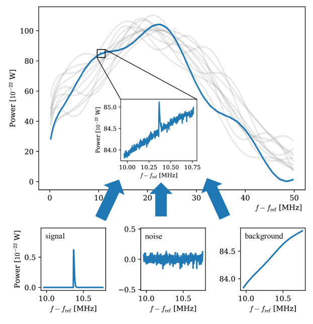
Figure 1: Components of a simulated example dataset. The upper panel shows multiple different datasets in order to visualise the variation in the simulated backgrounds, as well as a zoom into the region of the axion signal for one of them. The three lower panels contain the three components of a dataset: The simulated axion signal, uncorrelated noise and the background (from left to right).

III.2 Savitzky-Golay Filters

As stated above, obtaining a parametric background model for MADMAX data is likely not feasible. We thus have to rely on a non-parametric background estimator, suitable candidates being Savitzky-Golay filters.

Savitzky-Golay (SG) filters are a well-established and powerful smoothing technique often used for reducing noise in evenly spaced data while preserving the underlying smooth features [41]. The filter works by fitting low-degree polynomials to overlapping windows of data points using the method of least squares. The output of the filter is the value of the fitted polynomial at the central point of each window. The parameters of the filter are the windows length and degree of the polynomials. If these are chosen well for the given data, then SG filters can often suppress higher-frequency noise substantially while preserving the lower-frequency shape of the input. Improved versions and alternatives to SG filters have been proposed [42], but in our example use case we find that classical SG filters perform very well.

An SG filter can be expressed compactly using matrices. Given a data vector $X$ of length $N$, we can construct a smoothed version $f_{\mathrm{bg}}(X)$ using a convolution with the filter coefficients $C$:

$$f_{\mathrm{bg}}(X)=X\ast C.$$ (17)

The filter coefficients $C$ can be found by solving a linear least-squares problem. Let $A$ be a matrix of size $M\times(n+1)$, where $M$ is the (odd) window size and $n$ is the polynomial degree. Each element of $A$ is defined as:

$$A_{ij}=\left(i-\frac{M-1}{2}\right)^{j},$$ (18)

where $i=0,1,...,M-1$ and $j=0,1,...,n$. We can find the filter coefficients $C$ by solving the following linear least-squares problem:

$$C=(A^{T}A)^{-1}A^{T}$$ (19)

The first row of the resulting matrix $C$ contains the filter coefficients. Note that these coefficients are computed only once for a given window size and polynomial degree and can be used to filter the entire data vector $Y$, effectively circumventing the fitting problem and resulting in high numerical performance.

SG filters are finite impulse response (FIR) filters and applied by convolution of the coefficients $C$ and the input data vector $X$. They are therefore inherently linear and satisfy the condition in Eq. 8.

By applying the SG filter to the axion haloscope data, we separate the axion signal and noise from the background, which has lower frequency characteristics. We do this without constructing a parametric model for the background. But as the signal, in contrast to the noise, is positive and not zero-symmetric, a fraction of the signal becomes part of the background estimate. This results in a bias that we need to correct for.

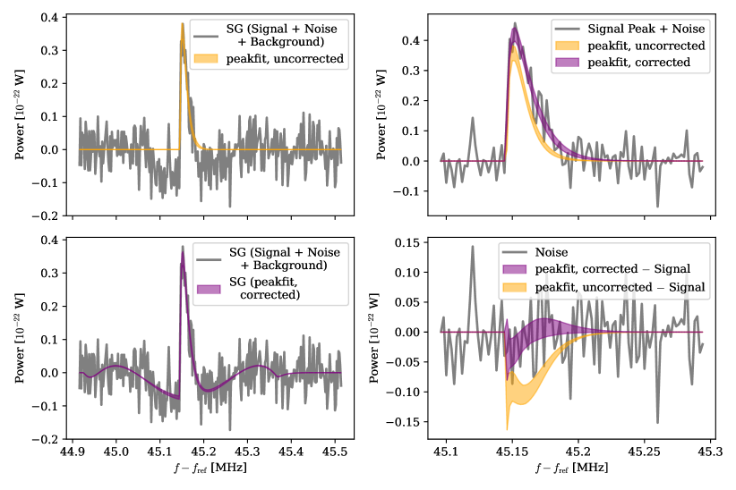
Figure 2: Effect of bias correction on the fit on the data. $68\%$ central posterior predictive intervals with and without using our bias correction procedure are plotted in purple and yellow respectively. Top Left: Data after background reduction via SG filter and uncorrected fit without SG filter applied. Bottom Left: Same data and corrected fit with SG filter applied. Top Right: Signal and noise components of the data as well as corrected and uncorrected peak-fit without applying an SG filter. Bottom Right: Deviation of posterior predictive of corrected and uncorrected peak-fit from the true signal compared to noise component of the data. The peak-fits in all panels have been performed on background reduced data as shown in the left panels. The data components shown in the right panels are for comparison only.

III.3 Demonstrating the Procedure

To test our bias correction approach on the problem stated above, we simulated 1000 MADMAX-like mock-datasets. A few of these are shown as grey lines in Fig. 1. We then analysed these datasets with and without bias correction. For our analysis we chose a Bayesian approach, however the bias correction procedure can be applied to (and is indeed also necessary for) other inference methods, e.g., a maximum likelihood estimate of the signal parameters.

The datasets consist of 25001 datapoints with $2$ kHz spacing. It has three components (see Fig. 1):

• Signal. An axion signal following the shape of Eq. 15. We assume fixed $\rho_{a}$ and $v_{\rm lab}$ and draw $m_{a}$, $\sigma_{v}$ and $E/N$ from the prior. For $E/N$ we additionally exclude models with $1.06<E/N<2.78$ to ensure that the signals are detectable at the noise level given below. So we’ll consider the scenario where an axion signal has been discovered but its quantitative properties have not been inferred yet.

• Noise. Uncorrelated Gaussian background noise with standard deviation $\sigma=5\times 10^{-24}$ W, corresponding to a realistic integration time below two weeks assuming noise temperatures below $10$ K.

• Background. Correlated, non-thermal background. Its shape is modelled by the following formula:

  $$\mathrm{b}(f)=10^{-20}\left[\mathrm{erf}\left(\frac{f-f_{0}}{5\,\mathrm{MHz}}\right)\left(\frac{f_{0}}{f}\right)^{3}\right.\\ +\left.\exp\left(-\left(\frac{f-25\,\mathrm{MHz}(1+\frac{r}{15})}{20\,\mathrm{MHz}(1+\frac{r}{10})}\right)^{2}\right)\right]\\ +4\times 10^{-22}(1+r)\sin\left(\frac{f+rf_{0}}{2.5\,\mathrm{MHz}}\right)\\ +5\times 10^{-24}\left[(1+r)\sin\left(\frac{f+rf_{0}}{0.25\,\mathrm{MHz}}\right)\right.\\ +\left.(1+r)\sin\left(\frac{f+rf_{0}}{0.1\,\mathrm{MHz}}\right)\right],$$ (20)

  where $f_{0}=4.218\,\mathrm{MHz}$ and $f$ are relative frequencies and all $r$ are independent random variables drawn from a Gaussian $\mathcal{N}(\mu=0,\sigma=1)$. The first three lines of Eq. 20 determine the large-scale shape of the background, but are easy to distinguish from an axion signal with a FWHM of roughly $10$ kHz. We therefore introduce two sine-like components with random phase, amplitudes of order of the uncorrelated noise and fixed periods of $100$ kHz and $250$ kHz.

Table 1: Overview over the fixed parameters in the analysis and the priors used for the three non-fixed parameters.

Parameter	Value/ Prior
$m_{a}$	Uniform$(f_{\rm min},f_{\rm max})$
$E/N$	From [37, 38], excluding $1.06<E/N<2.78$
$\sigma_{v}$	Normal$(218,39)$ [km s-1]
$\rho_{a}$	$0.3\,$GeV cm-3
$\beta^{2}$	$5\times 10^{4}$
$v_{\mathrm{lab}}$	$242\,$km s-1
$B_{e}$	$10\,$T
$A$	$1\,$m2

The relevant parameters for our analysis are summarised in Tab. 1. We filter the data consisting of these three components with a fourth-order SG filter of a width of $221$ datapoints, cutting away the first and last 110 datapoints due to boundary effects of the filter. Subtracting the filtered from the raw data removes the third, correlated background component almost completely, but also slightly distorts the signal shape, as shown below. The parameters of the SG fit were chosen to yield an optimal reduction of the background while leaving signal and noise almost unchanged.

Since we treat the amplitude of the uncorrelated noise as unknown we have to infer it from the data. If we would simply take the standard deviation of the background reduced data, the presence of a signal would lead to a slight bias for the noise towards higher values. To prevent the signal from biasing out noise-level estimation we first use the SG filter to remove a background estimate from the data. Then we partition each spectrum into three frequency regions of equal size: The localised signal can only be present in up to two of the pieces simultaneously. We select the region with the smallest standard deviation for our noise-level estimation. This removes the bias caused by the presence of the signal. In our test case the inferred noise level has a negligible difference compared to the ground truth.

For Monte Carlo analysis we use the reactive nested sampling algorithm [43, 44, 45] via the Bayesian Analysis Toolkit in Julia (BAT.jl)[46].

III.4 Results

Fig. 2 shows the result for one of the datasets. We demonstrate the effect of the bias correction qualitatively using $68$ percentile central posterior intervals. When the uncorrected signal model is used to fit the signal peak (Fig. 2, top left), the effect of the background reduction via SG filter cannot be modelled. Due to the presence of the signal, the background around the signal is overestimated, leading to a systematic decrease in signal height and adjacent datapoints below the baseline. A peak-fit is perfectly capable of fitting this modified signal, but cannot fit the surrounding datapoints - and therefore does not retain the true signal parameters. We will see this in the following.

The bottom-left plot in Fig. 2 shows the same, but with a corrected fit on the signal peak that takes the effect of SG filtering into account. We obtain a good fit over the whole frequency range, which displays the characteristic effect of an SG filter on the signal. Unbiased signal parameters can be obtained based on this fit, as Fig. 2, top right shows. The actual, non-filtered and background free signal peak is fitted well by the posterior predictive central interval of the corrected peak-fit on which no SG filter has been applied. The uncorrected peak-fit however underestimates signal height and width. This underestimation is made more visible in Fig. 2, bottom right, where the deviation relative to the true signal is shown in comparison with the noise level, both for the corrected and the uncorrected peak-fit. While the $68$ percentile of the corrected fit includes the true signal over almost the full frequency range, the uncorrected fit displays significant deviation.

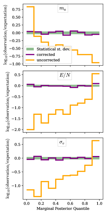
Figure 3: Distribution of the posterior quantiles in which the true signal resides for the three signal parameters, purple for the corrected peak-fit and orange for the uncorrected one. For 1000 mock-datasets and 10 quantile bins $100\pm 10$ cases are expected for each bin, which is shown as the green band. The distribution of the bias-corrected parameters shows no significant deviations from the expectation. Without the bias correction the posterior for the parameters display a significant and systematic shift away from the true signal. In this case almost all true signals reside in the first or last quantile of the posterior distribution.

We perform a coverage test to show that the analysis infers the correct parameters. From a Frequentist perspective, repeating an unbiased analysis multiple times should lead to the true signals being uniformly distributed over all marginal posterior quantiles. As we do have access to the ground truth of the signal parameters (using simulated data), and as we have 1000 equivalent mock-datasets at our disposal, we can verify our Bayesian results in this manner. The outcome is shown in Fig. 3. The uncorrected peak-fit that does not take the effect of the SG filter into account systematically underestimates $E/N$ and $\sigma_{v}$. It also shifts the axion mass to slightly larger values. The corrected fit, in comparison, shows no significant deviation from the expected uniform distribution and can therefore be considered unbiased.

IV Summary

We presented a method to fit small-amplitude signals on top of an unparameterised background in an unbiased fashion. The method is based on fairly weak assumptions about the problem, making it applicable in a wide variety of scenarios: we mainly require the existence of an unbiased and linear background estimator and an a-priori parameterisation of the signal. This enables us to virtually incorporate the background estimator into the measurement process and reduces to problem to model a background-free signal in the presence of symmetric noise, i.e., noise that has an expectation value of zero.

To evaluate the method in a practical real-world application, we applied it to signal estimation on simulated data for the planned MADMAX axion haloscope. The MADMAX experiment aims to detect a small, peaked axion dark matter signal in the presence of a challenging radio-frequency background that is difficult to model from first principles, so it is a very suitable candidate for the presented approach. For 1000 MADMAX-like mock datasets we used Savitzky-Golay filters as background estimators and inferred the signal parameter in a Bayesian fashion using nested sampling. The results verify the bias-correction approach presented here empirically and show that the signal parameter estimates are indeed unbiased. The true signal parameters are within the 68$\%$ central posterior predictive limits almost everywhere and the deviations of inferred parameters from the ground truth fell within the range of expected statistical fluctuations.

For comparison, we performed the signal parameter estimation without bias correction. Here the results do indeed show a significant systematic deviations from of the inferred signal parameters from the ground truth. The bias correction method is thus both effective and necessary.

- [1] ADMX Collaboration, C. Bartram et al., “Axion dark matter experiment: Run 1B analysis details,” Phys. Rev. D 103 no. 3, (2021) 032002, arXiv:2010.06183 [astro-ph.CO].
- [2] D. A. Palken et al., “Improved analysis framework for axion dark matter searches,” Phys. Rev. D 101 no. 12, (2020) 123011, arXiv:2003.08510 [astro-ph.IM].
- [3] F. Beaujean, A. Caldwell, and O. Reimann, “Is the bump significant? An axion-search example,” Eur. Phys. J. C 78 no. 9, (2018) 793, arXiv:1710.06642 [hep-ex].
- [4] MADMAX Working Group Collaboration, A. Caldwell, G. Dvali, B. Majorovits, et al., “Dielectric haloscopes: A new way to detect axion dark matter,” Phys. Rev. Lett. 118 (Mar, 2017) 091801. https://link.aps.org/doi/10.1103/PhysRevLett.118.091801.
- [5] A. J. Millar, G. G. Raffelt, J. Redondo, and F. D. Steffen, “Dielectric Haloscopes to Search for Axion Dark Matter: Theoretical Foundations,” JCAP 01 (2017) 061, arXiv:1612.07057 [hep-ph].
- [6] MADMAX Collaboration, P. Brun et al., “A new experimental approach to probe QCD axion dark matter in the mass range above 40 eV,” Eur. Phys. J. C 79 no. 3, (2019) 186, arXiv:1901.07401 [physics.ins-det].
- [7] S. Beurthey et al., “MADMAX Status Report,” arXiv:2003.10894 [physics.ins-det].
- [8] S. Weinberg, The quantum theory of fields. Vol. 2: Modern applications. 1996. http://www.slac.stanford.edu/spires/find/hep/www?key=3763846. Cambridge, UK: Univ. Pr. (1996) 489 p.
- [9] R. D. Peccei and H. R. Quinn, “ conservation in the presence of pseudoparticles,” Phys. Rev. Lett. 38 (Jun, 1977) 1440–1443. https://link.aps.org/doi/10.1103/PhysRevLett.38.1440.
- [10] R. D. Peccei and H. R. Quinn, “Constraints imposed by conservation in the presence of pseudoparticles,” Phys. Rev. D 16 (Sep, 1977) 1791–1797. https://link.aps.org/doi/10.1103/PhysRevD.16.1791.
- [11] S. Weinberg, “A new light boson?” Phys. Rev. Lett. 40 (Jan, 1978) 223–226. https://link.aps.org/doi/10.1103/PhysRevLett.40.223.
- [12] F. Wilczek, “Problem of Strong and Invariance in the Presence of Instantons,” Phys. Rev. Lett. 40 (1978) 279–282.
- [13] L. Abbott and P. Sikivie, “A cosmological bound on the invisible axion,” Physics Letters B 120 no. 1, (1983) 133–136. https://www.sciencedirect.com/science/article/pii/037026938390638X.
- [14] M. Dine and W. Fischler, “The not-so-harmless axion,” Physics Letters B 120 no. 1, (1983) 137–141. https://www.sciencedirect.com/science/article/pii/0370269383906391.
- [15] J. Preskill, M. B. Wise, and F. Wilczek, “Cosmology of the invisible axion,” Physics Letters B 120 no. 1, (1983) 127–132. https://www.sciencedirect.com/science/article/pii/0370269383906378.
- [16] GERDA Collaboration Collaboration, M. Agostini, A. M. Bakalyarov, M. Balata, et al., “First search for bosonic superweakly interacting massive particles with masses up to with gerda,” Phys. Rev. Lett. 125 (Jul, 2020) 011801. https://link.aps.org/doi/10.1103/PhysRevLett.125.011801.
- [17] EDELWEISS Collaboration Collaboration, E. Armengaud, C. Augier, A. Benoît, et al., “Searches for electron interactions induced by new physics in the edelweiss-iii germanium bolometers,” Phys. Rev. D 98 (Oct, 2018) 082004. https://link.aps.org/doi/10.1103/PhysRevD.98.082004.
- [18] QUAX Collaboration Collaboration, N. Crescini, D. Alesini, C. Braggio, et al., “Axion search with a quantum-limited ferromagnetic haloscope,” Phys. Rev. Lett. 124 (May, 2020) 171801. https://link.aps.org/doi/10.1103/PhysRevLett.124.171801.
- [19] XENON Collaboration Collaboration, E. Aprile, K. Abe, F. Agostini, et al., “Search for new physics in electronic recoil data from xenonnt,” Phys. Rev. Lett. 129 (Oct, 2022) 161805. https://link.aps.org/doi/10.1103/PhysRevLett.129.161805.
- [20] A. Garcon, J. W. Blanchard, G. P. Centers, et al., “Constraints on bosonic dark matter from ultralow-field nuclear magnetic resonance,” Science Advances 5 no. 10, (2019) eaax4539. https://www.science.org/doi/abs/10.1126/sciadv.aax4539.
- [21] JEDI Collaboration, S. Karanth et al., “First Search for Axion-Like Particles in a Storage Ring Using a Polarized Deuteron Beam,” arXiv:2208.07293 [hep-ex].
- [22] NASDUCK Collaboration, I. M. Bloch, R. Shaham, Y. Hochberg, et al., “NASDUCK SERF: New constraints on axion-like dark matter from a SERF comagnetometer,” arXiv:2209.13588 [hep-ph].
- [23] J. Lee, M. Lisanti, W. A. Terrano, and M. Romalis, “Laboratory constraints on the neutron-spin coupling of fev-scale axions,” Phys. Rev. X 13 (Mar, 2023) 011050. https://link.aps.org/doi/10.1103/PhysRevX.13.011050.
- [24] C. Hogan and M. Rees, “Axion miniclusters,” Physics Letters B 205 no. 2, (1988) 228–230. https://www.sciencedirect.com/science/article/pii/0370269388916553.
- [25] M. Buschmann, J. W. Foster, and B. R. Safdi, “Early-universe simulations of the cosmological axion,” Phys. Rev. Lett. 124 (Apr, 2020) 161103. https://link.aps.org/doi/10.1103/PhysRevLett.124.161103.
- [26] A. Vaquero, J. Redondo, and J. Stadler, “Early seeds of axion miniclusters,” Journal of Cosmology and Astroparticle Physics 2019 no. 04, (Apr, 2019) 012. https://dx.doi.org/10.1088/1475-7516/2019/04/012.
- [27] ADMX Collaboration, N. Du et al., “A Search for Invisible Axion Dark Matter with the Axion Dark Matter Experiment,” Phys. Rev. Lett. 120 no. 15, (2018) 151301, arXiv:1804.05750 [hep-ex].
- [28] ADMX Collaboration, T. Braine et al., “Extended Search for the Invisible Axion with the Axion Dark Matter Experiment,” Phys. Rev. Lett. 124 no. 10, (2020) 101303, arXiv:1910.08638 [hep-ex].
- [29] ADMX Collaboration, R. Khatiwada et al., “Axion Dark Matter Experiment: Detailed design and operations,” Rev. Sci. Instrum. 92 no. 12, (2021) 124502, arXiv:2010.00169 [astro-ph.IM].
- [30] ADMX Collaboration, C. Bartram et al., “Search for Invisible Axion Dark Matter in the 3.3–4.2 eV Mass Range,” Phys. Rev. Lett. 127 no. 26, (2021) 261803, arXiv:2110.06096 [hep-ex].
- [31] ADMX Collaboration, T. Nitta et al., “Search for the Cosmic Axion Background with ADMX,” arXiv:2303.06282 [hep-ex].
- [32] B. T. McAllister, G. Flower, E. N. Ivanov, et al., “The organ experiment: An axion haloscope above 15 ghz,” Physics of the Dark Universe 18 (2017) 67–72. https://www.sciencedirect.com/science/article/pii/S2212686417300602.
- [33] HAYSTAC Collaboration, L. Zhong et al., “Results from phase 1 of the HAYSTAC microwave cavity axion experiment,” Phys. Rev. D 97 no. 9, (2018) 092001, arXiv:1803.03690 [hep-ex].
- [34] HAYSTAC Collaboration, K. M. Backes et al., “A quantum-enhanced search for dark matter axions,” Nature 590 no. 7845, (2021) 238–242, arXiv:2008.01853 [quant-ph].
- [35] HAYSTAC Collaboration, M. J. Jewell et al., “New results from HAYSTAC’s phase II operation with a squeezed state receiver,” Phys. Rev. D 107 no. 7, (2023) 072007, arXiv:2301.09721 [hep-ex].
- [36] G. Grilli di Cortona, E. Hardy, J. Pardo Vega, and G. Villadoro, “The QCD axion, precisely,” JHEP 01 (2016) 034, arXiv:1511.02867 [hep-ph].
- [37] J. Diehl and E. Koutsangelas, “Dine-Fischler-Srednicki-Zhitnitsky-type axions and where to find them,” Phys. Rev. D 107 no. 9, (2023) 095020, arXiv:2302.04667 [hep-ph].
- [38] V. Plakkot and S. Hoof, “Anomaly ratio distributions of hadronic axion models with multiple heavy quarks,” Physical Review D 104 no. 7, (2021) 075017.
- [39] J. Bovy, C. A. Prieto, T. C. Beers, et al., “The milky way’s circular-velocity curve between 4 and 14 kpc from apogee data,” The Astrophysical Journal 759 no. 2, (2012) 131.
- [40] S. Knirck, A. J. Millar, C. A. J. O’Hare, et al., “Directional axion detection,” JCAP 11 (2018) 051, arXiv:1806.05927 [astro-ph.CO].
- [41] A. Savitzky and M. J. Golay, “Smoothing and differentiation of data by simplified least squares procedures.” Analytical chemistry 36 no. 8, (1964) 1627–1639.
- [42] M. Schmid, D. Rath, and U. Diebold, “Why and how savitzky–golay filters should be replaced,” ACS Measurement Science Au 2 no. 2, (2022) 185–196.
- [43] J. Buchner, “A statistical test for Nested Sampling algorithms,” Statistics and Computing 26 no. 1-2, (Jan., 2016) 383–392.
- [44] J. Buchner, “Collaborative Nested Sampling: Big Data versus Complex Physical Models,” Publications of the Astronomical Society of the Pacific 131 no. 1004, (Oct., 2019) 108005.
- [45] J. Buchner, “UltraNest - a robust, general purpose Bayesian inference engine,” The Journal of Open Source Software 6 no. 60, (Apr., 2021) 3001, arXiv:2101.09604 [stat.CO].
- [46] O. Schulz, F. Beaujean, A. Caldwell, et al., “Bat.jl: A julia-based tool for bayesian inference,” SN Computer Science 2 no. 3, (Apr, 2021) 210. https://doi.org/10.1007/s42979-021-00626-4.