First-passage time of a Brownian motion: two unexpected journeys

Abstract

The distribution of the first-passage time $T_{a}$ for a Brownian particle with drift $\mu$ subject to hitting an absorber at a level $a>0$ is well-known and given by its density $\gamma(t)=\frac{a}{\sqrt{2\pi t^{3}}}e^{-\frac{(a-\mu t)^{2}}{2t}},t>0$, which is normalized only if $\mu\geq 0$. In this article, we show that there are two other families of diffusion processes (the first with one parameter and the second with two parameters) having the same first passage-time distribution when $\mu<0$. In both cases we establish the propagators and study in detail these new processes. An immediate consequence is that the distribution of the first-passage time does not allow us to know if the process comes from a drifted Brownian motion or from one of these new processes.

Keywords: Stochastic particle dynamics (theory), Brownian motion

1 Introduction

Finding the distribution for the first time when a diffusion reaches a boundary [1, 2] is a fundamental quantity to characterize the process and has applications in many fields such as physics, chemistry, mathematical finance [3] and, more recently, biology, especially in the context of animal movement [4]. Quantities directly related to first-passage time like first-passage Brownian functionals are also widely studied [5, 6]. However, despite considerable efforts, some problems remain open, such as the first-passage time of the Ornstein-Uhlenbeck process, whose closed-form distribution is known only in the special case where the barrier is located at zero [7, 8].
In this article, our starting point is the drifted Brownian motion defined by its stochastic representation:

$$\left\{\begin{aligned} dX(t)&=\mu dt+\sqrt{2D}dW(t)\,,~{}~{}t\geq 0\\ X(0)&=0\,,\end{aligned}\right.$$ (1)

where $W(t)$ is a standard Brownian motion (Wiener process), $\mu$ the constant drift of the process and the diffusion parameter $D$ (which does not play any role in our study) is set to $1/2$. Let us denote by $T_{a}$ the stopping time:

$$T_{a}=\inf_{t\geq 0}\{t:X(t)=a\}\,,$$ (2)

where the barrier $a$, without loss of generality is positive. The first-passage time distribution of $T_{a}$ of this Brownian motion is well known and its density is given by [1]

$$\gamma(t)=\frac{a}{\sqrt{2\pi t^{3}}}e^{-\frac{(a-\mu t)^{2}}{2t}}\,,~{}~{}t>0,$$ (3)

and is normalized to unity only if $\mu\geq 0$. More precisely,

$$\int_{0}^{+\infty}\gamma(t)dt=\left\{\begin{array}[]{lll}1&~{}~{}\mathrm{if~{}~{}}\mu\geq 0\\ e^{-2|\mu|a}&~{}~{}\mathrm{if~{}~{}}\mu<0\,.\end{array}\right.$$ (6)

Now, we want to constrain the Brownian motion so that it has a new first-passage time distribution, again given by relation(3) but with a different parameter, say $\lambda\neq\mu$. In the recent article [11] we found out that when $\mu\geq 0$ and $\lambda\geq 0$ then the constrained process is merely a Brownian motion with drift $\lambda$, which is somewhat as expected. In this article, we are interested in the case where $\lambda<0$, and depending of the sign of $\mu$, we obtain quite surprising results since the drifts of the conditioned processes are both time- and space-dependent.

In order to tell this unexpected story, the paper is organized as follows: in Section 2 we recall what one needs to know about conditioning with respect to the first-passage time in order to derive the effective Langevin equations satisfied by the conditioned stochastic processes. Then, in section 3 we apply the formalism when the new distribution of the first-passage time is given by relation(3) with a negative parameter. In section 4 we solve analytically the effective stochastic Langevin equations using Girsanov’s theorem and we study the densities obtained. Finally, Section 5 presents some concluding remarks.

2 Conditioning with respect to the first-passage time, a brief remainder

In this section, we recall the essential ingredients to derive the stochastic differential equation for a diffusion conditioned by its first-passage time. This type of conditioning is a special case of conditioning with respect to a random time, whose general theory is still missing. To the best of our knowledge, the first work in this field is due to Baudoin [9] and was continued in  [10], but it is only very recently that conditioning with respect to first-passage time and the survival probability has been established [11].
In the following, we consider a Brownian motion with constant drift $\mu$ with absorbing condition at a position $a>0$. The unconditioned process $X(t)$ has the stochastic representation (1), whose propagator $P_{\mu}(x,t|0,0)=P_{\mu}(x,t)$ can be obtained by the method of images [1]

$$P_{\mu}(x,t)=\frac{1}{\sqrt{2\pi t}}\left(e^{-\frac{(x-\mu t)^{2}}{2t}}-e^{2\mu a}e^{-\frac{(x-2a-\mu t)^{2}}{2t}}\right),~{}~{}t>0\,.$$ (7)

With the propagator at our disposal, the distribution of the first-passage time follows easily [1, 11], its density is

$$\gamma(t)=\frac{a}{\sqrt{2\pi t^{3}}}e^{-\frac{(a-\mu t)^{2}}{2t}},~{}~{}t>0\,,$$ (8)

as well as the survival probability $S_{\mu}(t)$, which is the probability that the Brownian motion has not hit the absorbing boundary at time $t$. This quantity can be calculated in two ways, either with the propagator or with the first-passage time distribution [1]

$$S_{\mu}(t) =1-\int_{0}^{t}\gamma(s)ds=\int_{-\infty}^{a}P_{\mu}(x,t)dx$$

$$=\frac{1}{2}\left(1+\text{erf}\left(\frac{a-\mu t}{\sqrt{2t}}\right)-e^{2a\mu}\text{erfc}\left(\frac{a+\mu t}{\sqrt{2t}}\right)\right)\,$$ (9)

where $\operatorname{erf}(x)=\frac{2}{\sqrt{\pi}}\int_{0}^{x}du\,e^{-u^{2}}$ is the Error function and $\operatorname{erfc}(x)$ the complementary Error function $\operatorname{erfc}(x)=1-\operatorname{erf}(x)$. In particular, the forever-survival probability $S_{\mu}(\infty)$ vanished only for positive drift $\mu\geq 0$

$$S_{\mu}(\infty)=\left\{\begin{array}[]{lll}0&~{}~{}\mathrm{if~{}~{}}\mu\geq 0\\ 1-e^{-2|\mu|a}&~{}~{}\mathrm{if~{}~{}}\mu<0\,,\end{array}\right.$$ (12)

while for negative drift $\mu<0$, the particle can escape toward $(-\infty)$ without touching the absorbing boundary $a$ with the finite probability $S_{\mu}(\infty)=1-e^{-2|\mu|a}$. Now, we want to impose a new probability distribution for the first-passage time. From [11] we know that when the time horizon is infinite $T=+\infty$, the conditioning consists in imposing the new probability distribution with density $\gamma^{*}(t)$ of the absorption time $T_{a}\in[0,+\infty[$, whose normalization $[1-S^{*}(\infty)]$ determines the conditioned probability $S^{*}(\infty)\in[0,1]$ of the forever-survival. Thus, there are two conditions, and the effective Langevin equation of the conditioned process $X^{*}(t)$ is described by the following SDE:

$$X^{*}(t)=\mu^{*}(X^{*}(t),t)dt+dW(t)\,,~{}~{}t\geq 0,$$ (13)

where the conditioned drift $\mu^{*}(x,t)$ is given by

$$\mu^{*}(x,t)=\mu+\partial_{x}\ln Q(x,t)\,,$$ (14)

with the function

$$Q(x,t) =\int_{t}^{\infty}\gamma^{*}(s)\frac{\gamma(s|x,t)}{\gamma(s|x_{0},0)}ds$$ (15)

$$+S^{*}(\infty)\left[\lim_{T\to+\infty}\frac{S(\infty|x)+\int_{T}^{+\infty}\gamma(s|x,t)ds}{S(\infty|x_{0})+\int_{T}^{+\infty}\gamma(s|x_{0},0)ds}\right]\,,$$

containing all the information concerning the conditioning [11]. In the previous equation, $S(\infty|x)$ is the survival probability when starting at position $x$ and $\gamma(t|x,t)$ is the conditional probability density of the absorption-time $T_{a}$ knowing that the process started at the position $x$ at time $t$. Moreover, from its construction, $Q(x,t)$ inherits the backward Fokker-Planck dynamics of the initial process with respect to the initial variables $(x,t)$, that is

$$-\partial_{t}Q(x,t)=\mu\,\partial_{x}Q(x,t)+\frac{1}{2}\partial^{2}_{xx}Q(x,t)\,.$$ (16)

For more details, again we refer the reader to the paper [11] where the proofs are given as well as many examples. In particular, when

$$\gamma^{*}(t)=\frac{a}{\sqrt{2\pi t^{3}}}e^{-\frac{(a-\lambda t)^{2}}{2t}},~{}~{}t>0\mathrm{~{}~{}with~{}}\lambda~{}\geq 0\,,$$ (17)

and thus $S^{*}(\infty)=0$, the conditioned drift $\mu^{*}(x,t)$ reduces to $\lambda$, which is the expected result. From now on, we consider that the target first-passage density $\gamma^{*}(t)$ is given by Eq.(17) with $\lambda<0$ and we distinguish two cases depending on whether the initial drift $\mu$ is positive or strictly negative.

3 Conditioning with respect to the first-passage time density $\gamma^{*}(t)=\frac{a}{\sqrt{2\pi t^{3}}}e^{-\frac{(a-\lambda t)^{2}}{2t}}$ with $\lambda<0$

When conditioning toward a distribution of first-passage time whose density is not normalized to unity, the forever survival probability also plays a central role as established in [11]. The expression of $Q(x,t)$ given by Eq.(15) must be computed carefully and depends strongly on the sign of the initial drift $\mu$. Therefore, in the next two subsections, we distinguish the two cases, depending on whether the initial drift is zero or positive $\mu\geq 0$ or strictly negative $\mu<0$.

3.1 When the initial drift is vanishing or positive $\mu\geq 0$ (case I)

When the initial drift is $\mu\geq 0$, the conditional probability density $\gamma(s|x,t)$ of the absorption at time $T_{a}$ knowing that the process started at the position $x$ at time $t$ reads [1, 11]

$$\gamma(s|x,t)=\frac{(a-x)}{\sqrt{2\pi(s-t)^{3}}}e^{-\frac{(a-x-\mu(s-t))^{2}}{2(s-t)}}\,,~{}s>t\geq 0,$$ (18)

and the forever survival probability vanished $S(\infty|x)=S(\infty|0)=0$. Moreover, since

$$\gamma^{*}(t)=\frac{a}{\sqrt{2\pi t^{3}}}e^{-\frac{(a-\lambda t)^{2}}{2t}},~{}~{}t>0\,,$$ (19)

with $\lambda<0$, the forever survival probability associated is $S_{\lambda}^{*}(\infty)=(1-e^{2\lambda a})$. Reporting these expressions in Eq.(15), we get

$$Q_{I}(x,t) =\left(\frac{a-x}{a}\right)e^{-\mu x+\frac{\mu^{2}}{2}t}\left[\int_{t}^{+\infty}\frac{a}{\sqrt{2\pi s^{3}}}e^{\lambda a-\frac{a^{2}}{2s}-\frac{\lambda^{2}}{2}s}\left(\frac{s}{s-t}\right)^{\frac{3}{2}}e^{\frac{a^{2}}{2s}-\frac{(a-x)^{2}}{2(s-t)}}ds+(1-e^{2\lambda a})\right]$$

$$=\left(\frac{a-x}{a}\right)e^{-\mu x+\frac{\mu^{2}}{2}t}\left[\frac{a}{\sqrt{2\pi}}e^{\lambda a-\frac{\lambda^{2}}{2}t}\int_{t}^{+\infty}\left(\frac{1}{s-t}\right)^{\frac{3}{2}}e^{-\frac{\lambda^{2}}{2}(s-t)-\frac{(a-x)^{2}}{2(s-t)}}ds+(1-e^{2\lambda a})\right]$$

$$=\left(\frac{a-x}{a}\right)e^{-\mu x+\frac{\mu^{2}}{2}t}\left[\frac{a}{\sqrt{2\pi}}e^{\lambda a-\frac{\lambda^{2}}{2}t}\frac{\sqrt{2\pi}}{(a-x)}e^{\lambda(a-x)}+(1-e^{2\lambda a})\right]$$

$$=e^{-\mu x+\frac{\mu^{2}}{2}t+2\lambda a}\left[e^{-\lambda x-\frac{\lambda^{2}}{2}t}+(e^{-2\lambda a}-1)\left(\frac{a-x}{a}\right)\right]\,,$$ (20)

and the corresponding drift

$$\mu^{*}_{I}(x,t) =\mu+\partial_{x}\ln Q_{I}(x,t)$$

$$=\partial_{x}\ln\underbrace{\left[e^{-\lambda x-\frac{\lambda^{2}}{2}t}+(e^{-2\lambda a}-1)\left(\frac{a-x}{a}\right)\right]}_{\equiv\tilde{Q}_{I}(x,t)}$$

$$=\frac{e^{-\lambda x-\frac{\lambda^{2}}{2}t}(-\lambda)+(e^{-2\lambda a}-1)\left(-\frac{1}{a}\right)}{e^{-\lambda x-\frac{\lambda^{2}}{2}t}+(e^{-2\lambda a}-1)\left(\frac{a-x}{a}\right)}\,.$$ (21)

Consequently, the stochastic representation of conditioned process, that we will name $X_{I}(t)$, is not that of a Brownian motion with drift, $dX_{I}(t)=\lambda dt+dW(t)$ (as one might have expected) but obeys an inhomogeneous diffusion process

$$dX_{I}(t)=\left(\frac{e^{-\lambda X_{I}(t)-\frac{\lambda^{2}}{2}t}(-\lambda)+(e^{-2\lambda a}-1)\left(-\frac{1}{a}\right)}{e^{-\lambda X_{I}(t)-\frac{\lambda^{2}}{2}t}+(e^{-2\lambda a}-1)\left(\frac{a-X_{I}(t)}{a}\right)}\right)dt+dW(t)\,,~{}~{}t\geq 0\,,$$ (22)

which is independent of the initial drift $\mu$. Assuming that $X_{I}(t)$ remains finite, the long time behavior of the conditioned drift

$$\mu^{*}_{I}(x,t)\underset{t\to\infty}{\sim\,}-\frac{1}{a-x}$$ (23)

corresponds to the drift of a taboo process (with taboo state $a$) [13, 14, 15]. In particular, the boundary $a$ is no longer absorbing, but becomes a entrance boundary [16], which means that the boundary $a$ cannot be reach from the interior of the state space, .i.e the interval $]-\infty,a[$. Roughly speaking, after an arbitrarily large time $t$, the process can no longer be absorbed, which is the expected behavior.

3.2 When the initial drift is strictly negative $\mu<0$ (case II)

When the initial drift is strictly negative $\mu<0$, the conditional probability density $\gamma(s|x,t)$ of the absorption at time $T_{a}$, knowing that the process started at the position $x$ at time $t$, is still given by Eq.(18) but with a non vanishing forever survival probability $S(\infty|x)=1-e^{2\mu(a-x)}$ [1, 11]. Reporting these expressions in Eq.(15), we obtain

$$Q_{II}(x,t) =\int_{t}^{+\infty}\frac{a}{\sqrt{2\pi s^{3}}}e^{\lambda a-\frac{a^{2}}{2s}-\frac{\lambda^{2}}{2}s}\left(\frac{s}{s-t}\right)^{\frac{3}{2}}\left(\frac{a-x}{a}\right)e^{-\mu x+\frac{\mu^{2}}{2}t+\frac{a^{2}}{2s}-\frac{(a-x)^{2}}{2(s-t)}}ds$$

$$+(1-e^{2\lambda a})\left[\frac{1-e^{2\mu(a-x)}}{1-e^{2\mu a}}\right]$$

$$=\frac{(a-x)}{\sqrt{2\pi}}e^{\lambda a-\mu x+\frac{\mu^{2}-\lambda^{2}}{2}t}\int_{t}^{+\infty}\left(\frac{1}{s-t}\right)^{\frac{3}{2}}e^{-\frac{\lambda^{2}}{2}(s-t)-\frac{(a-x)^{2}}{2(s-t)}}ds+(1-e^{2\lambda a})\left[\frac{1-e^{2\mu(a-x)}}{1-e^{2\mu a}}\right]$$

$$=\frac{(a-x)}{\sqrt{2\pi}}e^{\lambda a-\mu x+\frac{\mu^{2}-\lambda^{2}}{2}t}\frac{\sqrt{2\pi}}{(a-x)}e^{\lambda(a-x)}+\frac{\left(1-e^{2a\lambda}\right)}{\left(1-e^{2a\mu}\right)}\left(1-e^{2\mu(a-x)}\right)$$

$$=e^{2a\lambda-\lambda x-\mu x+\frac{1}{2}\left(\mu^{2}-\lambda^{2}\right)t}+\frac{\left(1-e^{2a\lambda}\right)}{\left(1-e^{2a\mu}\right)}\left(1-e^{2\mu(a-x)}\right)\,,$$ (24)

and the corresponding drift

$$\mu^{*}_{II}(x,t) =\mu+\partial_{x}\ln Q_{II}(x,t)$$

$$=\mu+\partial_{x}\ln\left[e^{2a\lambda-\lambda x-\mu x+\frac{1}{2}\left(\mu^{2}-\lambda^{2}\right)t}+\frac{\left(1-e^{2a\lambda}\right)}{\left(1-e^{2a\mu}\right)}\left(1-e^{2\mu(a-x)}\right)\right]$$

$$=\mu+\frac{-(\lambda+\mu)e^{2a\lambda-\lambda x-\mu x+\frac{1}{2}\left(\mu^{2}-\lambda^{2}\right)t}+2\mu\frac{\left(1-e^{2a\lambda}\right)}{\left(1-e^{2a\mu}\right)}e^{2\mu(a-x)}}{e^{2a\lambda-\lambda x-\mu x+\frac{1}{2}\left(\mu^{2}-\lambda^{2}\right)t}+\frac{\left(1-e^{2a\lambda}\right)}{\left(1-e^{2a\mu}\right)}\left(1-e^{2\mu(a-x)}\right)}\,.$$ (25)

Observe that when $\lambda=\mu$ then $\mu^{*}(x,t)=\mu$ as it should. However, as in the case of a positive initial drift, the stochastic representation of conditioned process, that we will name $X_{II}(t)$, is not that of a Brownian motion with drift $\lambda$ (again as one might have expected) but obeys a rather complicated inhomogeneous diffusion process

$$dX_{II}(t) =\left(\mu+\frac{-(\lambda+\mu)e^{2a\lambda-\lambda X_{II}(t)-\mu X_{II}(t)+\frac{1}{2}\left(\mu^{2}-\lambda^{2}\right)t}+2\mu\frac{\left(1-e^{2a\lambda}\right)}{\left(1-e^{2a\mu}\right)}e^{2\mu(a-X_{II}(t))}}{e^{2a\lambda-\lambda X_{II}(t)-\mu X_{II}(t)+\frac{1}{2}\left(\mu^{2}-\lambda^{2}\right)t}+\frac{\left(1-e^{2a\lambda}\right)}{\left(1-e^{2a\mu}\right)}\left(1-e^{2\mu(a-X_{II}(t))}\right)}\right)dt$$

$$+dW(t)\,,~{}~{}t\geq 0\,,$$ (26)

which depends on both the initial drift $\mu$ and the new drift $\lambda$. Assuming that $X_{II}(t)$ remains finite, the long time behavior of the conditioned drift depends on the intensity of the two drifts, more precisely

$$\mu^{*}_{II}(x,t)\underset{t\to\infty}{\sim\,}\left\{\begin{array}[]{lll}-\mu\coth(\mu(a-x))&~{}~{}\mathrm{if~{}~{}}|\lambda|>|\mu|\\ -\lambda&~{}~{}\mathrm{if~{}~{}}|\lambda|<|\mu|\end{array}\right.$$ (29)

In the first case, $|\lambda|>|\mu|$, when $x$ approaches the boundary $a$, the conditioned drift behaves as

$$\mu^{*}_{II}(x,\infty)\mathop{\sim}_{x\to a^{-}}-\frac{1}{a-x}$$ (30)

which is the taboo drift we encountered previously and consequently, the conditioned process can never cross the barrier $a$. In the second case, when $|\lambda|<|\mu|$, the behavior is more surprising, even counter-intuitive, since for large times the conditioned drift $-\lambda$ is positive instead of negative. We can guess that during the intermediate times the process has been sent away from the barrier $a$, otherwise with a positive drift it will end up being absorbed at the boundary $a$ which is contrary to the initial hypothesis of having a positive survival probability. In the next paragraph, we will solve this weird behavior by calculating the probability densities of the conditioned processes.

4 Probability densities of the conditioned processes

In the previous paragraph, we left the reader in a puzzling yet interesting situation, with two unexpected conditioned drifts. To better understand the behavior of theses conditioned processes we seek their probability densities. However, solving Eq.(22) or Eq.(3.2) (or theirs corresponding Fokker-Planck equations) by a direct approach seems hopeless due to the space and time-inhomogeneous drifts. Therefore, we adopt a different strategy by resorting to Girsanov’s theorem whose derivation can be found, for example, in Karatzas and Shreve [17] or $\O$ksendal [18]. This theorem can be used to transform the probability measures of stochastic differential equations and, in particular, we will use it to remove the initial drift of Eqs.(22) and (3.2), with the hope that in this ”drift-free” world, calculations become feasible. Let us be more specific, and consider the Itô SDE

$$\left\{\begin{aligned} dX(t)&=\mu(X(t),t)dt+dW(t)\,,~{}~{}t\geq 0\\ X(0)&=x_{0}\,,\end{aligned}\right.$$ (31)

where $W(t)$ is a standard Brownian motion. Girsanov’s theorem tells us that the expectation of any function $h(X(t))$, where $X(t)$ is a solution of Eq.(31), can be express as [19]

$$E[h(X(t))]=E[Z(t)h(\underbrace{x_{0}+W(t)}_{\text{driftless process}})]\,.$$ (32)

with

$$Z(t)=e^{\textstyle\int_{0}^{t}\mu(x_{0}+W(t),t)dW(t)-\frac{1}{2}\int_{0}^{t}\mu(x_{0}+W(t),t)^{2}dt}\,.$$ (33)

Let us see what we get with the two drifts $\mu^{*}_{I}(x,t)$ and $\mu^{*}_{II}(x,t)$.

4.1 Probability density when the initial drift is vanishing or positive $\mu\geq 0$ (case I)

Reporting the expression of $\mu^{*}_{I}(x,t)$ into Eq.(33) leads to (recall that $x_{0}=0$ in our cases)

$$Z_{I}(t) =e^{\textstyle\int_{0}^{t}\mu^{*}_{I}(W(t),t)dW(t)-\frac{1}{2}\int_{0}^{t}\mu^{*}_{I}(W(t),t)^{2}dt}$$

$$=e^{\textstyle\int_{0}^{t}\left(\partial_{x}\log[\tilde{Q}_{I}(W(t),t)]\right)dW(t)-\frac{1}{2}\int_{0}^{t}\left(\partial_{x}\log[\tilde{Q}_{I}(W(t),t)]\right)^{2}dt}$$

$$=e^{\textstyle\int_{0}^{t}\frac{\partial_{x}\tilde{Q}_{I}(W(t),t)}{\tilde{Q}_{I}(W(t),t)}dW(t)-\frac{1}{2}\int_{0}^{t}\frac{(\partial_{x}\tilde{Q}_{I}(W(t),t))^{2}}{\tilde{Q}_{I}(W(t),t)^{2}}dt}$$ (34)

with (Eq.(3.1))

$$\left\{\begin{aligned} \tilde{Q}_{I}(x,t)&=e^{-\lambda x-\frac{\lambda^{2}}{2}t}+(e^{-2\lambda a}-1)\left(\frac{a-x}{a}\right)\\ \tilde{Q}_{I}(0,0)&=e^{-2\lambda a}\,.\end{aligned}\right.$$ (35)

The first integral can be evaluated thanks to Itô’s formula,

$$d\left[\log\left[\tilde{Q}_{I}(W(t),t)\right]\right] =d\left[\log\left[e^{-\lambda W(t)-\frac{\lambda^{2}}{2}t}+(e^{-2\lambda a}-1)\left(\frac{a-W(t)}{a}\right)\right]\right]$$

$$=\cancel{-\frac{\lambda^{2}}{2}\frac{e^{-\lambda W(t)-\frac{\lambda^{2}}{2}t}}{\tilde{Q}_{I}(W(t),t)}}dt+\frac{\partial_{x}\tilde{Q}_{I}(W(t),t)}{\tilde{Q}_{I}(W(t),t)}dW(t)$$

$$+\frac{1}{2}\left[\cancel{\frac{\lambda^{2}e^{-\lambda W(t)-\frac{\lambda^{2}}{2}t}}{\tilde{Q}_{I}(W(t),t)}}-\frac{(\partial_{x}\tilde{Q}_{I}(W(t),t))^{2}}{\tilde{Q}_{I}(W(t),t)^{2}}\right]dt\,.$$ (36)

Therefore, the first integral reads

$$\int_{0}^{t}\frac{\partial_{x}\tilde{Q}_{I}(W(t),t)}{\tilde{Q}_{I}(W(t),t)}dW(t)=\log\left[\tilde{Q}_{I}(W(t),t)\right]-\log\left[\tilde{Q}_{I}(0,0)\right]+\frac{1}{2}\int_{0}^{t}\frac{(\partial_{x}\tilde{Q}_{I}(W(t),t))^{2}}{\tilde{Q}_{I}(W(t),t)^{2}}dt\,.$$ (37)

Reporting this expression into Eq.(4.1), we obtain

$$Z_{I}(t) =e^{\textstyle\log\left[\tilde{Q}_{I}(W(t),t)\right]-\log\left[\tilde{Q}_{I}(0,0)\right]}$$

$$=e^{2\lambda a}\left[e^{-\lambda W(t)-\frac{\lambda^{2}}{2}t}+(e^{-2\lambda a}-1)\left(\frac{a-W(t)}{a}\right)\right]\,.$$ (38)

Since this expression depends solely on the state of the Brownian motion at time $t$, the probability density can be evaluated explicitly [19]. Recall that the probability density of the drift-less process $W(t)$ is given by Eq.(7) with $\mu=0$

$$P_{0}(x,t)=\frac{1}{\sqrt{2\pi t}}\left(e^{-\frac{x^{2}}{2t}}-e^{-\frac{(x-2a)^{2}}{2t}}\right)\,,~{}~{}t>0,$$ (39)

and thus from Eqs.(4.1) and (39) we obtain the probability density $p_{I}(x,t)$ of the conditioned process Eq.(22)

$$p_{I}(x,t)=e^{2a\lambda}\left(e^{-\lambda x-\frac{1}{2}\lambda^{2}t}+\left(e^{-2a\lambda}-1\right)\frac{(a-x)}{a}\right)\frac{1}{\sqrt{2\pi t}}\left(e^{-\frac{x^{2}}{2t}}-e^{-\frac{(x-2a)^{2}}{2t}}\right)\,,$$ (40)

which by construction satisfies the boundary condition

$$p_{I}(a,t)=0\,.$$ (41)

From the previous equation it is straightforward to verify that $p_{I}(x,t)$ satisfies the Fokker-Planck equation

$$\partial_{t}p_{I}(x,t)-\frac{1}{2}\partial_{xx}^{2}p_{I}(x,t)+\partial_{x}\left[\mu^{*}_{I}(x,t)p_{I}(x,t)\right]=0\,.$$ (42)

Besides, observe that the survival probability at time $t$

$$\int_{-\infty}^{a}p_{I}(x,t)dx =\int_{-\infty}^{a}e^{2a\lambda}\left(e^{-\lambda x-\frac{1}{2}\lambda^{2}t}+\left(e^{-2a\lambda}-1\right)\frac{(a-x)}{a}\right)\frac{1}{\sqrt{2\pi t}}\left(e^{-\frac{x^{2}}{2t}}-e^{-\frac{(x-2a)^{2}}{2t}}\right)dx$$

$$=\frac{1}{2}\left(1+\text{erf}\left(\frac{a-\lambda t}{\sqrt{2t}}\right)-e^{2a\lambda}\text{erfc}\left(\frac{a+\lambda t}{\sqrt{2t}}\right)\right)\,$$ (43)

is that of the Brownian motion with drift $\lambda$, (Eq.(2)), as it should.

4.2 Probability density when the initial drift is strictly negative $\mu<0$ (case II)

As in the previous case we proceed by inserting the expression of $\mu^{*}_{II}(x,t)$ in Eq.(33), so we get

$$Z_{II}(t) =e^{\textstyle\int_{0}^{t}\mu^{*}_{II}(W(t),t)dW(t)-\frac{1}{2}\int_{0}^{t}\mu^{*}_{II}(W(t),t)^{2}dt}$$

$$=e^{\textstyle\int_{0}^{t}\left(\mu+\partial_{x}\log[Q_{II}(W(t),t)]\right)dW(t)-\frac{1}{2}\int_{0}^{t}\left(\mu+\partial_{x}\log[Q_{II}(W(t),t)]\right)^{2}dt}$$ (44)

$$=e^{\textstyle\mu W(t)+\int_{0}^{t}\frac{\partial_{x}Q_{II}(W(t),t)}{Q_{II}(W(t),t)}dW(t)-\frac{1}{2}\mu^{2}t-\mu\int_{0}^{t}\frac{\partial_{x}Q_{II}(W(t),t)}{Q_{II}(W(t),t)}dt-\frac{1}{2}\int_{0}^{t}\frac{(\partial_{x}Q_{II}(W(t),t))^{2}}{Q_{II}(W(t),t)^{2}}dt}$$

with (Eq.(3.2))

$$\left\{\begin{aligned} Q_{II}(x,t)&=e^{2a\lambda-\lambda x-\mu x+\frac{1}{2}\left(\mu^{2}-\lambda^{2}\right)t}+\frac{\left(1-e^{2a\lambda}\right)}{\left(1-e^{2a\mu}\right)}\left(1-e^{2\mu(a-x)}\right)\\ Q_{II}(0,0)&=1\,.\end{aligned}\right.$$ (45)

The stochastic integral can be evaluated by applying the Itô formula

$$d\left[\log\left[Q_{II}(W(t),t)\right]\right] =\frac{\partial_{t}Q_{II}(W(t),t)}{Q_{II}(W(t),t)}dt+\frac{1}{2}\left[\frac{\partial_{xx}^{2}Q_{II}(W(t),t)}{Q_{II}(W(t),t)}-\frac{(\partial_{x}Q_{II}(W(t),t))^{2}}{Q^{2}_{II}(W(t),t)}\right]dt$$

$$+\frac{\partial_{x}Q_{II}(W(t),t)}{Q_{II}(W(t),t)}dW(t)$$ (46)

which reads,

$$\int_{0}^{t}\frac{\partial_{x}Q_{II}(W(t),t)}{Q_{II}(W(t),t)}dW(t) =\log\left[Q_{II}(W(t),t)\right]-\cancel{\log\left[Q_{II}(0,0)\right]}+\frac{1}{2}\int_{0}^{t}\frac{(\partial_{x}Q_{II}(W(t),t))^{2}}{Q_{II}(W(t),t)^{2}}dt$$

$$-\int_{0}^{t}\frac{\partial_{t}Q_{II}(W(t),t)}{Q_{II}(W(t),t)}dt-\frac{1}{2}\int_{0}^{t}\frac{\partial_{xx}^{2}Q_{II}(W(t),t)}{Q_{II}(W(t),t)}dt\,,$$ (47)

and the Eq.(4.2) becomes

$$Z_{II}(t) =e^{\textstyle\mu W(t)+\log\left[Q_{II}(W(t),t)\right]-\int_{0}^{t}\frac{\partial_{t}Q_{II}(W(t),t)}{Q_{II}(W(t),t)}dt-\frac{1}{2}\int_{0}^{t}\frac{\partial_{xx}^{2}Q_{II}(W(t),t)}{Q_{II}(W(t),t)}dt+\cancel{\frac{1}{2}\int_{0}^{t}\frac{(\partial_{x}Q_{II}(W(t),t))^{2}}{Q_{II}(W(t),t)^{2}}dt}}$$

$$\times e^{\textstyle-\frac{1}{2}\mu^{2}t-\mu\int_{0}^{t}\frac{\partial_{x}Q_{II}(W(t),t)}{Q_{II}(W(t),t)}dt\cancel{-\frac{1}{2}\int_{0}^{t}\frac{(\partial_{x}Q_{II}(W(t),t))^{2}}{Q_{II}(W(t),t)^{2}}dt}}$$

$$=Q_{II}(W(t),t)e^{\textstyle\mu W(t)-\frac{1}{2}\mu^{2}t}e^{-\int_{0}^{t}\overbrace{\left(\scriptstyle\frac{\partial_{t}Q_{II}(W(t),t)}{Q_{II}(W(t),t)}+\mu\frac{\partial_{x}Q_{II}(W(t),t)}{Q_{II}(W(t),t)}+\frac{1}{2}\frac{\partial_{xx}^{2}Q_{II}(W(t),t)}{Q_{II}(W(t),t)}\right)}^{=0\text{ by virtue of Eq.}\eqref{Qbackward}}dt}$$

$$=\left(e^{2a\lambda-\lambda W(t)-\mu W(t)+\frac{1}{2}\left(\mu^{2}-\lambda^{2}\right)t}+\frac{\left(1-e^{2a\lambda}\right)}{\left(1-e^{2a\mu}\right)}\left(1-e^{2\mu(a-W(t))}\right)\right)e^{\textstyle\mu W(t)-\frac{1}{2}\mu^{2}t}$$ (48)

As in case I, this expression depends only on the state of the Brownian motion at time $t$ and therefore the probability density $p_{II}(x,t)$ of the conditioned process can be evaluated explicitly, we obtain

$$p_{II}(x,t)=\left(e^{2a\lambda-\lambda x-\mu x+\frac{1}{2}\left(\mu^{2}-\lambda^{2}\right)t}+\frac{\left(1-e^{2a\lambda}\right)}{\left(1-e^{2a\mu}\right)}\left(1-e^{2\mu(a-x)}\right)\right)\frac{e^{\mu x-\frac{1}{2}\mu^{2}t}}{\sqrt{2\pi t}}\left(e^{-\frac{x^{2}}{2t}}-e^{-\frac{(x-2a)^{2}}{2t}}\right)$$ (49)

which by construction satisfies the boundary condition

$$p_{II}(a,t)=0\,.$$ (50)

From the previous equation it is straightforward to check that $p_{II}(x,t)$ satisfies the Fokker-Planck equation

$$\partial_{t}p_{II}(x,t)-\frac{1}{2}\partial_{xx}^{2}p_{II}(x,t)+\partial_{x}\left[\mu^{*}_{II}(x,t)p_{II}(x,t)\right]=0\,.$$ (51)

Figure 1 shows various density profiles for the three processes $p_{\mu}(x,t)$, $p_{I}(x,t)$ and $p_{II}(x,t)$ at different times and for two different parameters $\lambda$.

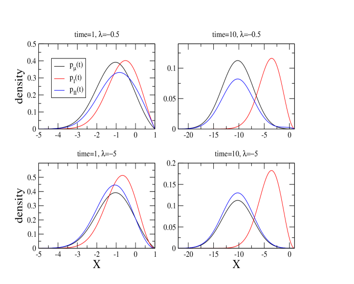
Figure 1: Examples of density profiles for the three processes: $p_{\mu}(x,t)$ given by Eq.(7) (black curve), $p_{I}(x,t)$ given by Eq.(40) (red curve) and $p_{II}(x,t)$ given by Eq.(49) (blue curve). For the densities $p_{\mu}(x,t)$ and $p_{II}(x,t)$ the parameter $\mu$ is equal to $-1$, thus the densities $p_{\mu}(x,t)$ are identical in each column since they depend only on $\mu$ and the time $t$. In the upper right figure, observe the plateaus in the density profile of $p_{II}(x,t)$ (blue curve) around $x\in[-2.5,0]$.

It is worth noting that while the probability density $p_{II}(x,t)$ depends on the two drifts $\mu$ and $\lambda$, it is remarkable that the survival probability at time $t$

$$\int_{-\infty}^{a}p_{II}(x,t)dx =\int_{-\infty}^{a}\left(e^{2a\lambda-\lambda x-\mu x+\frac{1}{2}\left(\mu^{2}-\lambda^{2}\right)t}+\frac{\left(1-e^{2a\lambda}\right)}{\left(1-e^{2a\mu}\right)}\left(1-e^{2\mu(a-x)}\right)\right)$$

$$\times\frac{e^{\mu x-\frac{1}{2}\mu^{2}t}}{\sqrt{2\pi t}}\left(e^{-\frac{x^{2}}{2t}}-e^{-\frac{(x-2a)^{2}}{2t}}\right)dx$$

$$=\frac{1}{2}\left(1+\text{erf}\left(\frac{a-\lambda t}{\sqrt{2t}}\right)-e^{2a\lambda}\text{erfc}\left(\frac{a+\lambda t}{\sqrt{2t}}\right)\right)$$ (52)

no longer depends on $\mu$, and is indeed that of the Brownian motion with $\lambda$ drift, (Eq. (2)), as it should.

From the propagators, it is straightforward to obtain the mean behavior of the three processes. We obtain respectively

$$\langle X_{\mu}(t)\rangle=\int_{-\infty}^{a}x\,P_{\mu}(x,t)dx =\int_{-\infty}^{a}x\,\frac{1}{\sqrt{2\pi t}}\left(e^{-\frac{(x-\mu t)^{2}}{2t}}-e^{2\mu a}e^{-\frac{(x-2a-\mu t)^{2}}{2t}}\right)dx$$ (53)

$$=\frac{1}{2}\left(\mu t\operatorname{erf}\left(\frac{a-\mu t}{\sqrt{2}\sqrt{t}}\right)-e^{2a\mu}(2a+\mu t)\operatorname{erfc}\left(\frac{a+\mu t}{\sqrt{2}\sqrt{t}}\right)+\mu t\right)$$

for an unconditioned Brownian motion with drift $\mu$,

$$\langle X_{I}(t)\rangle =\int_{-\infty}^{a}x\,P_{I}(x,t)dx=\int_{-\infty}^{a}x\,e^{2a\lambda}\left(e^{-\lambda x-\frac{1}{2}\lambda^{2}t}+\left(e^{-2a\lambda}-1\right)\frac{(a-x)}{a}\right)$$

$$\times\frac{1}{\sqrt{2\pi t}}\left(e^{-\frac{x^{2}}{2t}}-e^{-\frac{(x-2a)^{2}}{2t}}\right)dx$$

$$=\left(e^{2a\lambda}-1\right)\left(a+\frac{t}{a}\right)\operatorname{erf}\left(\frac{a}{\sqrt{2t}}\right)-2ae^{2a\lambda}+\sqrt{\frac{2t}{\pi}}\left(e^{2a\lambda}-1\right)e^{-\frac{a^{2}}{2t}}-\frac{1}{2}\lambda t\left(e^{2a\lambda}-1\right)$$

$$+\frac{1}{2}(2a-\lambda t)\operatorname{erf}\left(\frac{a-\lambda t}{\sqrt{2t}}\right)-\frac{1}{2}\lambda te^{2a\lambda}\operatorname{erf}\left(\frac{a+\lambda t}{\sqrt{2t}}\right)$$ (54)

for the type-I process, and

$$\langle X_{II}(t)\rangle =\int_{-\infty}^{a}x\,P_{II}(x,t)dx=\int_{-\infty}^{a}x\,\left(e^{2a\lambda-\lambda x-\mu x+\frac{1}{2}\left(\mu^{2}-\lambda^{2}\right)t}+\frac{\left(1-e^{2a\lambda}\right)}{\left(1-e^{2a\mu}\right)}\left(1-e^{2\mu(a-x)}\right)\right)$$

$$\times\frac{e^{\mu x-\frac{1}{2}\mu^{2}t}}{\sqrt{2\pi t}}\left(e^{-\frac{x^{2}}{2t}}-e^{-\frac{(x-2a)^{2}}{2t}}\right)dx$$

$$=\frac{1}{4}(\coth(a\mu)-1)\bigg{[}\left(1-e^{2a\mu}\right)\left(e^{2a\lambda}(2a+\lambda t)-\lambda t\right)$$

$$+\lambda t\left(e^{2a\lambda}-e^{2a(\lambda+\mu)}\right)\operatorname{erf}\left(\frac{a+\lambda t}{\sqrt{2}\sqrt{t}}\right)+\left(e^{2a\mu}-1\right)(2a-\lambda t)\operatorname{erf}\left(\frac{a-\lambda t}{\sqrt{2}\sqrt{t}}\right)$$

$$+2\left(e^{2a\lambda}-1\right)\left(e^{2a\mu}(a+\mu t)\operatorname{erf}\left(\frac{a+\mu t}{\sqrt{2}\sqrt{t}}\right)+(\mu t-a)\operatorname{erf}\left(\frac{a-\mu t}{\sqrt{2}\sqrt{t}}\right)\right)\bigg{]}$$ (55)

for the type-II process. For large times $t$, one can compute the leading order of the three previous expressions

$$\left\{\begin{aligned} \langle X_{\mu}(t)\rangle&\underset{t\to\infty}{\sim\,}\mu\left(1-e^{2a\mu}\right)t\\ \langle X_{I}(t)\rangle&\underset{t\to\infty}{\sim\,}-2\sqrt{\frac{2}{\pi}}\left(1-e^{2a\lambda}\right)\sqrt{t}\\ \langle X_{II}(t)\rangle&\underset{t\to\infty}{\sim\,}\mu\left(1-e^{2a\lambda}\right)t\,.\end{aligned}\right.$$ (56)

At large times, the average behavior of the unconditioned Brownian motion with drift $\mu$ and the average behavior of the type-II process behave like drifted Brownian motions with effective drift coefficients equal to $\lambda\left(1-e^{2a\lambda}\right)$ and $\mu\left(1-e^{2a\lambda}\right)$ respectively. Observe that if $|\mu|>|\lambda|$ then at large times, the average behavior of the type-II process ”goes” toward $-\infty$ slower that the unconditioned Brownian motion with drift $\lambda$ as shown in Fig. 2. Moreover, due to the square-root term of time, no matter the values of $\mu$ and $\lambda$, at large times, the average behavior of the type-I process remains closer to the boundary $a$ than the other two processes.

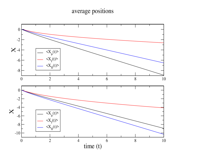
Figure 2: Examples of average behaviors of the three processes: the process $X_{\mu}(t)$ given by Eq.(53), the type-I process given by Eq.(4.2) and the type-II process given by Eq.(4.2). Top figure $\mu=-1$ and $\lambda=-0.5$. Bottom figure $\mu=-1$ and $\lambda=-5$. Note that the black curve is the same in both figures since $\mu$ is identical.

5 Discussion

Conditioned stochastic processes have sometime unexpected behaviors. Indeed, in this article we have conditioned the first-passage time distribution of a Brownian motion with drift $\mu$ starting at the origin with absorbing condition at a position $a>0$ towards the first-passage time distribution which would have another Brownian motion of drift $\lambda$. Recently Krapivsky and Redner [20] observed that when one conditions on the event that the particle surely reaches the absorbing boundary $a$, then the distribution of the first-passage time is independent of the direction of the external flow field. They called this phenomenon the first-passage duality. However, when one drops the hitting condition, the situation becomes more subtle and the conditioned drift $\mu^{*}(x,t)$ depends on the sign of $\mu$ and $\lambda$ as follows:

1. If $\mu\in\mathbb{R}$ and $\lambda\geq 0$ then $\mu^{*}(x,t)=\lambda$ is independent of the initial drift (first-passage duality).

2. If $\mu\geq 0$ and $\lambda<0$ then $\mu^{*}(x,t)=\mu_{I}^{*}(x,t)$ is independent of the initial drift, so we are still in first-passage duality configuration, but somewhat in a weaker form since the conditioned drift depends of the drift $\lambda$ as well as time and position.

3. If $\mu<0$ and $\lambda<0$ then $\mu^{*}(x,t)=\mu_{II}^{*}(x,t)$ depends of both the initial drift $\mu$ and the drift $\lambda$, as well as time and position (no first-passage duality).

The first-passage duality property recently discovered by Krapivsky and Redner [20] is always exact when we condition a Brownian motion with drift on a final density distribution which is independent of the initial drift [10]. However, in the present article we have established that conditioning a Brownian motion with drift on a random time, such as the first-passage time can break the first-passage duality property. In short, when the final drift is $\lambda<0$, so that there is some loss of information since the particle does not reach the boundary with a strictly positive probability and we do not impose where it might be, we should no longer expect to recover $\mu^{*}(x,t)=\lambda$.

In this article we have discovered two families of diffusion processes, the first with one parameter (the type-I process) and the second with two parameters (the type-II process) having the same first-passage time distribution as that of a Brownian motion whose drift is directed away from the absorbing boundary. This is rather unexpected and it would be very interesting to experimentally observe our predictions on real systems.

6 Acknowledgements

These two unexpected journeys are dedicated to the memory of Jérôme Combe.
The author is also grateful to Pr. Jordan Stoyanov for his well-intended and truly helpful comments.

References

• [1] Redner S, A Guide to First-Passage Processes, Cambridge University Press, Cambridge (2001).
• [2] Redner S, A first look at first-passage processes, Physica A: Statistical Mechanics and its Applications, 128545 (2023).
• [3] Metzler R., Redner S., and Oshanin G. (Eds.) First-passage phenomena and their applications (Vol. 35). World Scientific (2014).
• [4] McKenzie H. W., Lewis M. A., and Merrill E. H., First passage time analysis of animal movement and insights into the functional response, Bulletin of mathematical biology, 71, 107-129 (2009).
• [5] Majumdar S. N. and Meerson, B., Statistics of first-passage Brownian functionals, Journal of Statistical Mechanics: Theory and Experiment, 2020(2), 023202.
• [6] Majumdar S. N., Brownian functionals in physics and computer science, The Legacy Of Albert Einstein: A Collection of Essays in Celebration of the Year of Physics pp 93-129 (2007).
• [7] Alili L., Patie P. and Pedersen J. L., Representations of the first hitting time density of an Ornstein-Uhlenbeck process, Stochastic Models, 21(4) 967–980 (2005).
• [8] Ricciardi L. M. and Sato S., First-passage-time density and moments of the Ornstein-Uhlenbeck process, Journal of Applied Probability, 25(1) 43–57 (1988).
• [9] Baudoin, F.: Conditioned stochastic differential equations: Theory, Examples and Application to Finance, Stoch. Proc. Appl. 100, 109-145 (2002).
• [10] Larmier C., Mazzolo A. and Zoia A., Strongly constrained stochastic processes: the multi-ends Brownian bridge, Journal of Statistical Mechanics: Theory and Experiment, 2019(11), 113208.
• [11] Monthus C. and Mazzolo A., Conditioned diffusion processes with an absorbing boundary condition for finite or infinite horizon, Physical Review E, 106(4), 044117 (2022).
• [12] S.N. Majumdar and H. Orland, Effective Langevin equations for constrained stochastic processes, J. Stat. Mech. P06039 (2015).
• [13] Knight F.B., Brownian local times and taboo processes, Trans. Amer. Soc. 73, 173–185 (1969).
• [14] R.G. Pinsky, On the convergence of diffusion processes conditioned to remain in a bounded region for large time to limiting positive recurrent diffusion processes, Ann. Probab. 13(2), 363-378 (1985).
• [15] Mazzolo A., Sweetest taboo processes, J. Stat. Mech. P073204 (2018).
• [16] Karlin S. and Taylor H., A Second Course in Stochastic Processes, Academic Press, New York (1981).
• [17] Karatzas I. and Shreve S., Brownian motion and stochastic calculus (Vol. 113), Springer Science & Business Media (1991).
• [18] $\O$ksendal B., Stochastic differential equations: an introduction with applications, Springer Science & Business Media (2013).
• [19] Särkkä S. and Solin A., Applied stochastic differential equations, Cambridge University Press (2019).
• [20] Krapivsky P. L. and Redner S., First-passage duality, J. Stat. Mech. 093208 (2018).