Upscaling and Effective Behavior for Two-Phase Porous-Medium Flow using a Diffuse Interface Model

Abstract

We investigate two-phase flow in porous media and derive a two-scale model, which incorporates pore-scale phase distribution and surface tension into the effective behavior at the larger Darcy scale. The free-boundary problem at the pore scale is modeled using a diffuse interface approach in the form of a coupled Allen-Cahn Navier-Stokes system with an additional momentum flux due to surface tension forces. Using periodic homogenization and formal asymptotic expansions, a two-scale model with cell problems for phase evolution and velocity contributions is derived. We investigate the computed effective parameters and their relation to the saturation for different fluid distributions, in comparison to commonly used relative permeability saturation curves. The two-scale model yields non-monotone relations for relative permeability and saturation. The strong dependence on local fluid distribution and effects captured by the cell problems highlights the importance of incorporating pore-scale information into the macro-scale equations.

1 Introduction

Flow through porous media, especially in multi-phase systems, is of interest in a variety of applications from oil recovery and $CO_{2}$ sequestration to fuel cells and biological systems. Traditionally these are modeled using extended Darcy’s law for two phases, which lacks the mathematical derivation from pore-scale information available for the single-phase Darcy’s law. Single-phase Darcy’s law can be derived from a pore-scale model of (Navier-)Stokes equations through upscaling procedures. For two phases Darcy’s law has been extended by introducing empirically derived relative permeability saturation curves to capture fluid interactions. The effective behavior depends only on the averaged saturation and the model fails to capture different pore-scale effects. Further empiric modifications such as play-type hysteresis have been added to account for missing behavior. In this work we start from a two-phase-flow model at the pore scale and through appropriate assumptions and a periodic homgenization approach, we derive a two-scale model of macroscopic Darcy’s law-type equations with effective parameters computed from solutions of resulting pore-scale cell problems.

The flow of the two fluids is modeled on the pore scale using quasi-compressible Navier-Stokes equations with phase-dependent density and viscosity as well as an additional term capturing surface tension forces at the fluid-fluid interface. For the pore-scale model with resolved phase distribution we use a diffuse interface approach in the form of an Allen-Cahn phase-field model [allen1979]. Where a sharp-interface model separates the pore space into subdomains for each fluid phase, our approach captures the interface implicitly through a smooth phase field function. All unknowns are defined and modified equations hold on the entire domain of the pore space. This removes the need to track or capture the interface and decompose the domain in the numeric simulation. To resolve the transition zone between the two bulk phases a fine discretization is required near the interface, requiring high computational effort in the absence of adaptive local mesh refinement. Furthermore the Allen-Cahn model used in this work is not conservative, including a curvature driven motion of the interface. While the conservative Cahn-Hilliard model requires solving a fourth order partial differential equation, we consider the second order Allen-Cahn equation, which offers a much simpler numerical implementation, and we investigate the two-scale model derived from it. While there are different approaches to ensuring conservation of the phase field [bringedal2020con] or counteracting this curvature-driven motion entirely [xu2012], we apply the scaled mobility approach presented in [abels2021non] to eliminate the curvature-driven motion only in the sharp-interface limit. A core advantage of the diffuse interface approach is the ease of upscaling the equations, as they are defined on a stationary domain encompassing both fluid phases. In contrast, upscaling a sharp-interface model requires special attention to the evolving domains [vanNoorden2009].

The model is presented for two phases but extends well to more evolving phases [kelm2022, redecker2016], only a non-neutral contact angle at internal triple points between phases requires more attention [rohde2021].

To bridge the scale gap between pore scale and the averaged Darcy scale we employ the method of formal asymptotic homogenization [hornung1997homogenization]. Representing the porous medium by a periodic arrangement of scaled reference cells, one introduces an additional spatial coordinate for this smaller scale. Here the macroscopic scale corresponds to the Darcy scale and the microscopic scale is the pore scale. These two scales are sufficiently separated, with representative length scales $L$ and $\ell$ respectively defining a length scale ratio $\epsilon=\ell/L\ll 1$. Assuming asymptotic expansions of the unknowns in terms of $\epsilon$, considering the limit $\epsilon\to 0$ and grouping by orders of $\epsilon$, one obtains equations that are defined on the macro scale and form micro-scale cell problems. The former contains effective parameters which are computed from the cell problem unknowns, linking the two scales. Through the cell problems, these parameters and the effective behavior depend additionally on the distribution of fluids and are able to capture more detailed effects on the fluid velocities.

The homogenization leads to macroscopic equations similar to the extended Darcy’s law but with effective parameters computed from solutions of cell problems instead of being given by empiric relations. These effective parameters can be understood as total phase mobilities and for isotropic pore geometries a relative permeability can be computed. Through the cell problems these relative permeabilities in the two-scale model depend on the local phase distribution at the pore scale. This motivates a comparison of computed relative permeabilities to commonly used functional relations, enabling us to investigate under which conditions the models agree and which additional pore-scale effects are captured by the two-scale model. We investigate numerically the effective parameters computed for different geometries and fluid properties. Constructing fluid distributions of varying saturations, we solve the cell problems for the velocity contributions to obtain a relative permeability curve. The models are implemented using a staggered finite volume discretization in DuMu^x[KOCH2021423], with Dune-SPGrid [nolte2011] and Dune-Subgrid [graeser2009] used for the grid.

In [daly2015], [metzger2021], and [sharmin2022] a Cahn-Hilliard model was used to derive a similar two-scale model. We instead investigate the applicability of the simpler Allen-Cahn model and the effects of micro-scale information on the effective flow parameters. The derivation of a two-scale model in [metzger2021] additionally assumes a separation of time scales and a different asymptotic expansion to arrive at an instationary problem for the phase distribution. We use the full expansion in the spatial separation $\epsilon$ instead and afterwards introduce an artifical evolution to obtain a local phase distribution. In [daly2015] three time scales are used to separate interface equilibration, macroscopic flow and saturation changes. In [sharmin2022] a solute-dependent surface tension is considered and simulations of the coupled two-scale model are presented. We instead focus on a systematic investigation of the effective parameters computed from the cell problems. A similar comparison of effective parameters is included in [lasseux2022], where a sharp-interface Stokes model for two-phase flow is upscaled using volume averaging. However, [lasseux2022] does not account for a three-phase contact line or slip velocities at the solid, which are accounted for in the current work.

In this contribution we aim to derive a two-scale model for two-phase flow in porous media, which captures effects of pore-scale fluid distribution and surface tension on the effective behavior at the macro-scale. Our goal is to determine conditions under which the computed effective parameters show significantly different behavior to commonly used saturation-dependent curves and highlight the importance of resolving pore-scale behavior through a two-scale model for two-phase porous-medium flow.

The structure of this paper is as follows. We present our pore-scale model for two-phase flow using an Allen-Cahn formulation coupled to a modified Navier-Stokes system in Section 2. In Section 3 we perform the upscaling and obtain a two-scale model using periodic homogenization. We investigate the dependence of computed effective parameters on pore-scale conditions using DuMu^xin Section 4. Section 5 summarizes the derived model and relates it to the extended Darcy’s law.

2 Pore-scale modeling

We begin by presenting the pore-scale model describing two-phase flow. The model is first presented in a sharp-interface formulation before we introduce the diffuse-interface description for the phase-field model.

The general domain is a stationary void space inside a porous medium. We consider a domain $\Omega=\mathcal{P}\cup\mathcal{G}$ decomposed into a domain $\mathcal{P}$ capturing the pore space and the solid matrix $\mathcal{G}$. Here the distribution of two fluid phases needs to be captured and evolved according to the flow of the fluids, including effects of surface tension at the fluid-fluid interface.

2.1 Sharp-interface model

Figure 1: Interfaces and triple point.

The model is first formulated with a sharp interface separating the fluid phases and corresponding evolving subdomains $\Omega_{\alpha}(t)\subset\mathcal{P}$, $\alpha=1,2$ of the stationary pore space $\mathcal{P}$ (Figure 1). The interfaces between the fluid phases, denoted by ${\Gamma_{f}}(t)=\overline{\Omega_{1}(t)}\cap\overline{\Omega_{2}(t)}$, as well as the fluid-solid interfaces $\Gamma_{\alpha}=\overline{\Omega_{\alpha}}\cap\mathcal{G}$ evolve accordingly. Within each subdomain the flow is modelled using incompressible Navier-Stokes equations, with constant viscosity $\mu_{\alpha}$ and density $\rho_{\alpha}$.

$$\nabla\cdot\mathbf{v}_{\alpha} =0~{}, \text{ in }\Omega_{\alpha}~{},$$ (1)

$$\rho_{\alpha}\frac{\partial}{\partial t}\mathbf{v}_{\alpha}+\rho_{\alpha}\nabla\cdot(\mathbf{v}_{\alpha}\otimes\mathbf{v}_{\alpha}) =-p_{\alpha}+\mu_{\alpha}\nabla^{2}\mathbf{v}_{\alpha}+\rho_{\alpha}\mathbf{g}~{}, \text{ in }\Omega_{\alpha}~{}.$$ (2)

At the interfaces $\Gamma_{\alpha}$ with the solid matrix we prescribe a Navier-Slip [thalakkottor2016] boundary condition with slip length $\lambda\geq 0$ for the velocity $\mathbf{v}_{\alpha}$

$$\mathbf{v}_{\alpha}=-\lambda(\partial_{\mathbf{n}}\mathbf{v}_{\mathbf{t}})\mathbf{t}~{},\qquad\text{on }\Gamma_{\alpha}~{},$$ (3)

where $\mathbf{t}$ is tangential to the fluid-solid interface $\partial\mathcal{G}$. At the fluid-fluid interface ${\Gamma_{f}}$ we prescribe continuity of velocities with a no-slip condition enforcing zero tangential velocity, with interface velocity $V_{\Gamma_{f}}$ in the direction of the interface normal $\mathbf{n}_{\Gamma_{f}}$ pointing from fluid 1 into fluid 2,

$$\mathbf{v}_{\alpha}=V_{\Gamma_{f}}\mathbf{n}_{\Gamma_{f}}~{}.$$ (4)

The interface itself moves due to the local velocity of the fluids and with surface tension $\gamma$ and curvature $H_{\Gamma_{f}}$ we have a jump condition

$$[-p_{\alpha}\mathbf{I}+\mu_{\alpha}(\nabla\mathbf{v}_{\alpha}+(\nabla\mathbf{v}_{\alpha})^{T}-\frac{2}{3}\nabla\cdot\mathbf{v}_{\alpha}\mathbf{I})]\mathbf{n}_{\Gamma_{f}}=-\gamma H_{\Gamma_{f}}\mathbf{n}_{\Gamma_{f}}\qquad\text{on }{\Gamma_{f}}~{},$$ (5)

where $[\psi]=\psi_{1}-\psi_{2}$ denotes the jump over the interface. At the three-phase contact point the fluid-fluid-interface meets the solid with a contact angle $\theta_{\mathrm{eq}}$ (Figure 1). In a sharp-interface formulation this could be incorporated using a boundary condition for a level set equation, when a level set is used to track the location of the fluid-fluid-interface.

2.2 Phase-field model

To model two-phase flow at the pore scale we use a diffuse-interface approach, capturing the distribution of phases with a phase-field function $u$ defined on the total void space $u:T\times\mathcal{P}\to[0,1]$ with $u=0$ and $u=1$ corresponding to the two distinct phases $\alpha=2$ and $\alpha=1$ respectively. The phase-field variable evolves according to an advective Allen-Cahn equation, a second order partial differential equation (PDE) with a non-linear source term. The multi-phase system is then modeled as one fluid with varying properties, depending on $u(t,\mathbf{x})$ to account for phase distribution.

We use the compressible Navier-Stokes equations for non-constant viscosity, derived from conservation laws using Stokes hypothesis $\zeta=0$. A surface tension flux is added to the momentum equation, coupling it to the Allen-Cahn equation as presented for the stationary Stokes equation in [abels2018]. In [abels2012] the surface tension term is introduced to a Navier-Stokes equation with a phase field evolved according to the Cahn-Hilliard equation.

The resulting Navier-Stokes equations in conservative form are

$$\frac{\partial\rho}{\partial t}+\nabla\cdot(\rho\mathbf{v}) =0 \text{ in }\mathcal{P}~{},$$ (6a)

$$\frac{\partial}{\partial t}(\rho\mathbf{v})+\nabla\cdot(\rho\mathbf{v}\otimes\mathbf{v}) =-\nabla p+\nabla\cdot\left(\mu\left(\nabla\mathbf{v}+(\nabla\mathbf{v})^{T}-\frac{2}{3}(\nabla\cdot\mathbf{v})\mathbf{I}\right)\right)+\rho\mathbf{g}$$ (6b)

$$\phantom{=}-\frac{3}{2}\xi\gamma\nabla\cdot(\nabla u\otimes\nabla u) \text{ in }\mathcal{P}~{}.$$

We focus on the case of each fluid being incompressible, treating the multiphase system as a quasi-incompressible fluid with density and viscosity dependent on the present phase in a linear manner. Denoting mass and viscosity ratios $R=\rho_{1}/\rho_{2}$ and $M=\mu_{1}/\mu_{2}$, we write

$$\rho(u) =\rho_{1}u+\rho_{2}(1-u)=\rho_{2}+u(\rho_{1}-\rho_{2})=\rho_{2}\left(1+u\left(\frac{\rho_{1}}{\rho_{2}}-1\right)\right)=\rho_{2}(1+u(R-1))~{},$$ (7a)

$$\mu(u) =\mu_{1}u+\mu_{2}(1-u)=\mu_{2}(1+u(M-1))~{}.$$ (7b)

This is combined with the advective Allen-Cahn equation, additionally coupled via the advecting velocity and the surface tension momentum flux. The phase-field equation is given as

$$\frac{\partial u}{\partial t}+\nabla\cdot(\mathbf{v}u)=\sigma\xi(\nabla^{2}u-\xi^{-2}P^{\prime}(u))\,,\quad\text{in }\mathcal{P}\,,\quad P(u)=8u^{2}(1-u)^{2}~{},$$ (8)

where we consider the scaled diffusivity $\sigma\xi$ suggested in [abels2021non] in order to obtain a more favorable sharp-interface limit. The diffusivity $\sigma$ and diffuse-interface width $\xi$ prescribe how strongly a certain profile is enforced for the transition zone between bulk phases and the width of this zone respectively. The double-well potential, $P(u)$, encourages a separation of phases through stable minima at $u=0$ and $u=1$.

The (no-)slip boundary conditions on solid boundaries apply also here, with interpolation based on the phase-field $u$ if phase-dependent slip lengths are desired. Additionally for the phase-field a Neumann boundary condition encoding the contact angle $\theta_{\mathrm{eq}}$ measured through fluid 1, corresponding to $u=1$ (Fig 2), is prescribed [frank2018, lunowa2021].

Figure 2: Contact angle boundary condition for the diffuse-interface phase-field model.

$$\mathbf{v} =-\lambda(\partial_{\mathbf{n}}\mathbf{v}_{\mathbf{t}})\mathbf{t}~{}, \text{ on }\partial\mathcal{P}~{},$$ (9a)

$$\partial_{\mathbf{n}}u =-\cos(\theta_{\mathrm{eq}})\xi^{-1}\sqrt{2P(u)}~{}, \text{ on }\partial\mathcal{P}~{}.$$ (9b)

Note that for vanishing slip length $\lambda=0$ and for neutral contact angle $\theta_{\mathrm{eq}}=\frac{\pi}{2}$, the boundary conditions reduce to homogeneous Dirichlet and Neumann conditions for velocity and phase field respectively. The Appendix A includes the sharp-interface limit of the coupled Navier-Stokes Allen-Cahn system presented in this section, yielding again the sharp-interface model presented in Section 2.1.

3 Upscaling using periodic homogenization

Starting from the diffuse-interface model from Section 2.2, describing the phase distribution and flow at the pore scale, we derive effective equations capturing the behavior at the Darcy scale. At the same time we obtain a set of micro-scale cell problems, defined at each macroscopic point, the solutions of which allow the computation of effective tensors. These are then used as parameters to the macro-scale problem, which in turn supplies global pressure gradients and saturations used by the cell problems, arriving at a coupled two-scale problem. As will be shown, these effective parameters can be interpreted as phase mobilities.

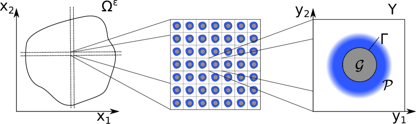
Figure 3: Separation of scales and domain definitions

To achieve this we assume a sufficient separation of scales, with characteristic length scales $\ell$ for the pore scale and $L$ for the Darcy scale at which we are interested in the effective behavior. Assuming a scale separation $\epsilon=\ell/L\ll 1$, we first non-dimensionalize the model. We then follow the approach of periodic homogenization, modeling the porous medium as a periodic arrangement of scaled reference cells $\epsilon Y$, $Y=[0,1]^{\mathrm{d}}$ with dimension $\mathrm{d}$, where $\mathrm{d}$ is 2 or 3, (see Figure 3). The domain of the porous medium is thus decomposed into $\Omega^{\epsilon}=\cup_{w\in W_{\Omega}}\,\epsilon(w+Y)$, with $W_{\Omega}\in\mathbb{Z}^{\mathrm{d}}$ a set of indices. With local pore space and solid matrix denoted as $Y=\mathcal{P}\cup\mathcal{G}$ and the outer boundary of the reference cell given as $\partial Y$ we denote the interior boundary between solid and fluid as

$$\Gamma=\overline{\mathcal{P}}\cap\mathcal{G}~{}.$$ (10)

The global pore space and its boundary with the solid matrix in the non-dimensional case is then given as

$$\mathcal{P}^{\epsilon}=\cup_{w\in W_{\Omega}}\,\epsilon(w+\mathcal{P})~{},\quad\Gamma^{\epsilon}=\cup_{w\in W_{\Omega}}\,\epsilon(w+\Gamma)~{}.$$ (11)

While their fluid content can generally vary between the cells, we here assume that the porous matrix is constant both in time and space in order to facilitate the derivation of the two-scale model. As the reference cell is the unit cube, we can define the constant porosity $\varphi=|\mathcal{P}|$. The conditions inside the pore spaces still vary, with fluid saturations and distributions changing in time and between cells.

We use the scale separation to introduce a micro-scale coordinate, rewrite spatial derivatives accordingly, assign scalings in terms of $\epsilon$ for the dimensionless numbers and assume all unknowns to have an asymptotic expansion in $\epsilon$. Inserting the expansions into the model equations and gathering terms of equal order in terms of $\epsilon$ we obtain a new set of equations containing derivatives with respect to coordinates of only one of the spatial scales. This procedure yields macroscopic equations capturing the effective behavior and cell problems defined on the reference cell. Effective parameters are defined through cell problems and integrals of their solutions, linking the two sets of equations and capturing detailed effects of local phase distribution on effective behavior. In addition to pressure driven flow, a separate cell problem captures flow due to surface tension forces, reflected in an added velocity contribution on the effective scale.

3.1 Non-dimensionalization

In preparation of upscaling by periodic homogenization we non-dimensionalize the micro-scale model. The homogenization requires a separation of scales between representative length $\ell$ at the pore scale and the length scale of interest $L$ at the macro scale, quantified by the small number $\epsilon=\ell/L\ll 1$. Defining reference values with dimensions

$$[\hat{L}] =\mathrm{m} [\hat{\ell}] =\mathrm{m} [\hat{\xi}] =\mathrm{m} [\hat{t}] =\mathrm{s} [\hat{v}] =\mathrm{\frac{m}{s}}$$

$$[\hat{\rho}] =\mathrm{\frac{kg}{m^{3}}} [\hat{\mu}] =\mathrm{\frac{kg}{m\cdot s}} [\hat{p}] =\mathrm{\frac{kg}{m\cdot s^{2}}} [\hat{}\lambda] =\mathrm{m} [\hat{}\sigma] =\mathrm{\frac{m}{s}}~{},$$

and letting

$$\hat{L} =L \hat{\ell} =\ell \hat{\xi} =\hat{\ell} \hat{t} =\frac{\hat{L}}{\hat{v}} \hat{\rho} =\rho_{2} \hat{\mu} =\mu_{2} \hat{}\lambda =\hat{\ell} \hat{}\sigma =\sigma~{},$$ (12)

one can rewrite the phase-field model equations using non-dimensional variables and parameters

$$\bar{\xi} =\frac{\xi}{\hat{\xi}} \bar{}\mathbf{v} =\frac{\mathbf{v}}{\hat{v}} \bar{\rho} =\frac{\rho}{\hat{\rho}} \bar{\mu} =\frac{\mu}{\hat{\mu}} \bar{p} =\frac{p}{\hat{p}} \bar{t} =\frac{t}{\hat{t}} \bar{}\lambda =\frac{\lambda}{\hat{\lambda}}~{}.$$

In the following all variables and parameters are non-dimensional and the overline notation is dropped for convenience. Using dimensionless numbers

$$\mathrm{Re}\, =\frac{\hat{\rho}\hat{v}\hat{L}}{\hat{\mu}} \mathrm{Ca}\, =\frac{\hat{v}\hat{\mu}}{\gamma} \mathrm{Eu} =\frac{\hat{p}}{\hat{\rho}\hat{v}^{2}} \mathrm{Fr} =\frac{\hat{v}}{\sqrt{g\hat{L}}} S =\frac{\hat{}\sigma}{\hat{v}}~{},$$

one obtains (see Appendix B for details)

$$\frac{\partial\rho}{\partial t}+\nabla\cdot(\rho\mathbf{v}) =0 ~{},\text{ in }\mathcal{P}~{},$$ (13a)

$$\frac{\partial}{\partial t}(\rho\mathbf{v})+\nabla\cdot(\rho\mathbf{v}\otimes\mathbf{v}) =-\mathrm{Eu}\nabla p+\frac{1}{\mathrm{Re}\,}\nabla\cdot\left(\mu\left(\nabla\mathbf{v}+(\nabla\mathbf{v})^{T}-\frac{2}{3}(\nabla\cdot\mathbf{v})\mathbf{I}\right)\right)$$ (13b)

$$\phantom{=}-\frac{1}{\mathrm{Fr}^{2}}\rho\mathbf{z}-\frac{\epsilon}{\mathrm{Ca}\,}\frac{3\xi}{2}\nabla\cdot(\nabla u\otimes\nabla u) ~{},\text{ in }\mathcal{P}~{},$$

with boundary conditions

$$\mathbf{v}=-\epsilon\lambda(\partial_{\mathbf{n}}\mathbf{v}_{\mathbf{t}})\mathbf{t}~{},\text{ on }\Gamma$$ (14)

For the phase-field equation the non-dimensionalization yields (see Appendix B for details)

$$\frac{\partial u}{\partial t}-S\epsilon^{1}\xi\nabla^{2}u+\nabla\cdot(\mathbf{v}u)=-S\epsilon^{-1}\xi^{-1}P^{\prime}(u)~{},\text{ in }\mathcal{P}~{},$$ (15)

with boundary condition

$$\partial_{\mathbf{n}}u=-\epsilon^{-1}\xi^{-1}\cos(\theta_{\mathrm{eq}})\sqrt{2P(u)}~{},\text{ on }\Gamma~{}.$$ (16)

Phase-constant density and viscosity

Using the above equations (7) for density and viscosity and the reference values (12), the non-dimensional viscosity and density in (13) are

$$\mu(u)= \frac{1}{\hat{\mu}}(\mu_{1}u+\mu_{2}(1-u))=1+u(M-1)~{},$$ (17)

$$\rho(u)= 1+u(R-1)~{}.$$ (18)

3.2 Periodic Homogenization

Given the scale separation $\epsilon$ we introduce the micro-scale coordinate $\mathbf{y}=\epsilon^{-1}\mathbf{x}$ and assume all unknowns can be written as an asymptotic expansion in $\epsilon$, depending on both $\mathbf{x}$ and $\mathbf{y}$ with periodicity in the unit cell $Y$. For an unknown $\psi\in\{p,\mathbf{v},u\}$ we introduce $Y$-periodic $\psi_{k}(t,\mathbf{x},\mathbf{y})$ such that

$$\psi(t,\mathbf{x})=\sum_{k=0}^{\infty}\epsilon^{k}\psi_{k}\left(t,\mathbf{x},\frac{\mathbf{x}}{\epsilon}\right)~{}.$$

The spatial derivatives are rewritten as

$$\nabla\psi=\nabla_{\mathbf{x}}\sum_{k=0}^{\infty}\epsilon^{k}\psi_{k}(t,\mathbf{x},\mathbf{y})+\frac{1}{\epsilon}\nabla_{\mathbf{y}}\sum_{k=0}^{\infty}\epsilon^{k}\psi_{k}(t,\mathbf{x},\mathbf{y})~{}.$$

For the upscaling we consider a flow regime where Darcy’s law is considered valid, with laminar flow driven by the pressure drop and capillary forces, and where advective and diffusive time scales are of the same order. For the phase distribution the phase-field diffusivity $\sigma$ should be comparable to the micro-scale advection, captured by $S\in\mathcal{O}(\epsilon^{0})$. As will be shown in Remark 1, with $S\in\mathcal{O}(\epsilon^{1})$ the advective term separates in the upscaling process and yields a restrictive pore-scale equation as well as introducing mixed-scale derivatives into the phase-field equation. Choosing non-dimensional numbers $\mathrm{Ca}\,\in\mathcal{O}(\epsilon^{0})$, $\mathrm{Re}\,\in\mathcal{O}(\epsilon^{0})$, $\mathrm{Eu}\in\mathcal{O}(\epsilon^{-2})$ and $\mathrm{Fr}\in\mathcal{O}(\epsilon^{0})$ the leading terms for $\epsilon\to 0$ are given as follows (see Appendix C for details).

For the phase dependent fluid properties we observe

$$\mu(u) =(1+u(M-1))=\underbrace{1+u_{0}(M-1)}_{=\mu(u_{0})}+\epsilon u_{1}(M-1)+\mathcal{O}(\epsilon^{2})$$ (19a)

$$\rho(u) =(1+u(R-1))=\underbrace{1+u_{0}(R-1)}_{=\rho(u_{0})}+\epsilon\underbrace{u_{1}(R-1)}_{=\rho_{1}}+\mathcal{O}(\epsilon^{2})~{},$$ (19b)

and for the double-well potential of the phase-field equation, due to its polynomial structure,

$$P^{\prime}(u) =P^{\prime}(u_{0})+\epsilon u_{1}P^{\prime\prime}(u_{0})+\mathcal{O}(\epsilon^{2})~{}.$$ (19c)

Denoting $\overline{\mathrm{Eu}}:=\epsilon^{2}\mathrm{Eu}$, we have for (13a), (13b) and (15) in $\mathcal{P}$

$$\mathcal{O}(\epsilon^{1})= \epsilon^{-1}\nabla_{\mathbf{y}}\cdot(\rho(u_{0})\mathbf{v}_{0})$$ (20a)

$$+\epsilon^{0}\bigg{[}\frac{\partial\rho(u_{0})}{\partial t}+\nabla_{\mathbf{y}}\cdot(\rho(u_{0})\mathbf{v}_{1}+\rho_{1}\mathbf{v}_{0})+\nabla_{\mathbf{x}}\cdot(\rho(u_{0})\mathbf{v}_{0})\bigg{]}$$

$$\mathcal{O}(\epsilon^{-1})= \epsilon^{-3}\left[-\overline{}\mathrm{Eu}\nabla_{\mathbf{y}}p_{0}\right]$$ (20b)

$$+\epsilon^{-2}\bigg{[}-\overline{}\mathrm{Eu}(\nabla_{x}p_{0}+\nabla_{\mathbf{y}}p_{1})$$

$$+\frac{1}{\mathrm{Re}\,}\nabla_{\mathbf{y}}\cdot\left(\mu(u_{0})\left(\nabla_{\mathbf{y}}\mathbf{v}_{0}+(\nabla_{\mathbf{y}}\mathbf{v}_{0})^{T}-\frac{2}{3}(\nabla_{\mathbf{y}}\cdot\mathbf{v}_{0})I\right)\right)$$

$$-\frac{1}{\mathrm{Ca}\,}\frac{3\xi}{2}\nabla_{\mathbf{y}}\cdot(\nabla_{\mathbf{y}}u_{0}\otimes\nabla_{\mathbf{y}}u_{0})\bigg{]}$$

$$\mathcal{O}(\epsilon^{1})= \epsilon^{-1}[\nabla_{\mathbf{y}}\cdot(\mathbf{v}_{0}u_{0})-S\xi\nabla_{\mathbf{y}}^{2}u_{0}+S\xi^{-1}P^{\prime}(u_{0})]$$ (20c)

$$+\epsilon^{0}\bigg{[}\frac{\partial u_{0}}{\partial t}+\nabla_{\mathbf{y}}\cdot(\mathbf{v}_{1}u_{0}+\mathbf{v}_{0}u_{1})+\nabla_{\mathbf{x}}\cdot(\mathbf{v}_{0}u_{0})+S\xi^{-1}P^{\prime\prime}(u_{0})u_{1}$$

$$-S\xi(\nabla_{\mathbf{y}}\cdot\nabla_{\mathbf{x}}u_{0}+\nabla_{\mathbf{x}}\cdot\nabla_{\mathbf{y}}u_{0}+\nabla_{\mathbf{y}}^{2}u_{0})\bigg{]}$$

and for boundary conditions (14) and (16) on $$\Gamma$$

$$\mathcal{O}(\epsilon^{1}) =\epsilon^{0}\Big{[}\mathbf{v}_{0}+\lambda(\nabla_{\mathbf{y}}\mathbf{v}_{0,\mathbf{t}}\cdot\mathbf{n})\mathbf{t}\Big{]}$$ (20d)

$$\mathcal{O}(\epsilon^{0}) =\epsilon^{-1}\Big{[}\nabla_{\mathbf{y}}u_{0}\cdot\mathbf{n}+\xi^{-1}\cos(\theta_{\mathrm{eq}})\sqrt{2P(u_{0})}\Big{]}~{}.$$ (20e)

3.2.1 Phase field

From the leading order term of (20c) we therefore obtain a stationary equation involving only local derivatives.

$$-S\xi\nabla_{\mathbf{y}}^{2}u_{0}+\nabla_{\mathbf{y}}\cdot(\mathbf{v}_{0}u_{0})=S\xi^{-1}P^{\prime}(u_{0})~{},\qquad\text{ in }\mathcal{P}~{},$$ (21)

together with boundary condition (20e)

$$\nabla_{\mathbf{y}}u_{0}\cdot\mathbf{n}=-\xi^{-1}\cos(\theta_{\mathrm{eq}})\sqrt{2P(u_{0})}~{},\qquad\text{ on }\Gamma~{}.$$ (22)

Remark 1.

If the phase-field equation is dominated by advection ($S\in\mathcal{O}(\epsilon^{1})$) the leading order advective term of (20e) would be isolated at $\mathcal{O}(\epsilon^{-2})$ as

$$\nabla_{\mathbf{y}}\cdot(\mathbf{v}_{0}u_{0})=0~{}.$$ (23)

Applied to the leading order term in (20a) this yields a divergence free velocity field and reduces to

$$\mathbf{v}_{0}\cdot\nabla_{\mathbf{y}}u_{0}=0~{},$$ (24)

resulting in a strong limitation on modeled problems. At the order $\mathcal{O}(\epsilon^{-1})$ the equation (20c) would instead contain the advective terms of the next order, yielding

$$0=\nabla_{\mathbf{y}}\cdot(\mathbf{v}_{1}u_{0}+\mathbf{v}_{0}u_{1})+\nabla_{\mathbf{x}}\cdot(\mathbf{v}_{0}u_{0})-S\xi\nabla_{\mathbf{y}}^{2}u_{0}+S\xi^{-1}P^{\prime}(u_{0})$$ (25)

with an undesireable mix of scales that leads to neither a pore-scale cell problem nor an effective equation for the Darcy scale. A balance of the two terms is expressed by $S\in\mathcal{O}(1)$, which yields (21) instead of (23) as the leading order equation.

This local phase-field equation (21) is underconstrained, admitting among others the trivial solutions of $u_{0}=0$ and $u_{1}=1$ for divergence free velocity fields. The local cell problem does not offer a way to compute the saturation of fluid 1 as the mean integral of $u_{0}$ but rather requires it as a constraint as in [sharmin2022].

From the next order $\mathcal{O}(\epsilon^{0})$ terms of the phase-field equation (20c) we obtain

$$0 =\frac{\partial u_{0}}{\partial t}-S\xi(\nabla_{\mathbf{y}}^{2}u_{1}+\nabla_{\mathbf{y}}\cdot(\nabla_{\mathbf{x}}u_{0})+\nabla_{\mathbf{x}}\cdot(\nabla_{\mathbf{y}}u_{0}))$$ (26)

$$\phantom{=}+(\nabla_{\mathbf{y}}\cdot(\mathbf{v}_{1}u_{0}+\mathbf{v}_{0}u_{1})+\nabla_{\mathbf{x}}\cdot(\mathbf{v}_{0}u_{0}))+S\xi^{-1}P^{\prime\prime}(u_{0})u_{1}~{}.$$

We would like to use this instationary equation to update the saturation to in turn constrain the stationary phase-field equation obtained from the leading order term of the asymptotic expansion. After integrating over the constant local periodicity cell $\mathcal{P}$ and using the periodicity with respect to $\mathbf{y}$, (26) reduces to

$$\frac{\partial}{\partial t}\int_{\mathcal{P}}u_{0}\,\mathrm{d}\mathbf{y}+\nabla_{\mathbf{x}}\cdot\int_{\mathcal{P}}\mathbf{v}_{0}u_{0}\,\mathrm{d}\mathbf{y}+\int_{\mathcal{P}}\frac{S}{\xi}P^{\prime\prime}(u_{0})u_{1}\,\mathrm{d}\mathbf{y}=0~{}.$$ (27)

While the first two terms yield a macroscopic equation in saturation and phase-specific velocity, the last term includes the additional unknown $u_{1}$. Assuming a homogeneous porous medium, with $\mathcal{P}$ not depending on $\mathbf{x}$, one can use a solvability constraint to show that this term is zero and obtain the desired saturation equation.

Integrating the leading order terms (21) and applying the divergence theorem and periodicity conditions, one is left with only the potential derivative.

$$0=\underbrace{\int_{\mathcal{P}}-S\xi\nabla_{\mathbf{y}}\cdot(\nabla_{\mathbf{y}}u_{0})+\nabla_{\mathbf{y}}\cdot(\mathbf{v}_{0}u_{0})\,\mathrm{d}\mathbf{y}}_{=0}+\int_{\mathcal{P}}\frac{S}{\xi}P^{\prime}(u_{0})\,\mathrm{d}\mathbf{y}$$ (28)

One now views the third term in (27) as a Fredholm operator of index zero $\mathcal{L}(u_{0})$ applied to $u_{1}$. Applying it instead to $\nabla_{\mathbf{x}}u_{0}$, using the chain rule and the assumption of $\mathcal{P}$ not depending on $\mathbf{x}$, we obtain

$$\mathcal{L}(u_{0})(\nabla_{\mathbf{x}}u_{0})=\int_{\mathcal{P}}\frac{S}{\xi}P^{\prime\prime}(u_{0})\nabla_{\mathbf{x}}u_{0}\,\mathrm{d}\mathbf{y}=\int_{\mathcal{P}}\frac{S}{\xi}\nabla_{\mathbf{x}}(P^{\prime}(u_{0}))\,\mathrm{d}\mathbf{y}=\frac{S}{\xi}\nabla_{\mathbf{x}}\int_{\mathcal{P}}P^{\prime}(u_{0})\,\mathrm{d}\mathbf{y}~{}.$$ (29)

Together with the previously derived information about $P^{\prime}$ from (28), one sees that $\nabla_{\mathbf{x}}u_{0}$ is an element of the kernel of $\mathcal{L}(u_{0})$. Rewriting (27) as $-\mathcal{L}(u_{0})u_{1}=A(u_{0},\mathbf{v}_{0})$ with

$$A(u_{0},\mathbf{v}_{0})=\int_{\mathcal{P}}\frac{\partial u_{0}}{\partial t}+\nabla_{\mathbf{x}}\cdot(\mathbf{v}_{0}u_{0})\,\mathrm{d}\mathbf{y}~{},$$ (30)

this yields the solvability constraint

$$0=<A(u_{0},\mathbf{v}_{0}),\nabla_{\mathbf{x}}u_{0}>=\int_{\Omega}\nabla_{\mathbf{x}}u_{0}(\mathbf{x},\mathbf{y})\left(\int_{\mathcal{P}}\frac{\partial u_{0}}{\partial t}+\nabla_{\mathbf{x}}\cdot(\mathbf{v}_{0}u_{0})\,\mathrm{d}\mathbf{y}\right)(\mathbf{x})\,\mathrm{d}\mathbf{x}~{}.$$ (31)

To avoid trivial behavior ($\nabla_{\mathbf{x}}u_{0}\equiv 0$, $\nabla_{\mathbf{x}}u_{0}$ independent of $\mathbf{x}$), the integral over the local pore-space $\mathcal{P}$ must disappear. Using again the assumption of a stationary and homogeneous pore space $\mathcal{P}$ with constant porosity $\varphi$, this yields the saturation equation

$$\frac{\partial}{\partial t}\int_{\mathcal{P}}u_{0}\,\mathrm{d}\mathbf{y}+\nabla_{\mathbf{x}}\cdot\int_{\mathcal{P}}\mathbf{v}_{0}u_{0}\,\mathrm{d}\mathbf{y}=0~{}.$$ (32)

Introducing averaged quantities for the saturation of fluid 1, $S^{(1)}=\varphi^{-1}\int_{\mathcal{P}}u_{0}\,\mathrm{d}\mathbf{y}$, as well as velocities

$$\bar{}\mathbf{v}^{(1)}=\varphi^{-1}\int_{\mathcal{P}}u_{0}\mathbf{v}_{0}\,\mathrm{d}\mathbf{y}~{},\qquad\bar{}\mathbf{v}^{(2)}=\varphi^{-1}\int_{\mathcal{P}}(1-u_{0})\mathbf{v}_{0}\,\mathrm{d}\mathbf{y}~{},\qquad\bar{}\mathbf{v}=\varphi^{-1}\int_{\mathcal{P}}\mathbf{v}_{0}\,\mathrm{d}\mathbf{y}~{},$$ (33)

we obtain

$$\frac{\partial}{\partial t}\int_{\mathcal{P}}u_{0}\,\mathrm{d}\mathbf{y}+\nabla_{\mathbf{x}}\cdot\int_{\mathcal{P}}\mathbf{v}_{0}u_{0}\,\mathrm{d}\mathbf{y}=\varphi\left(\frac{\partial}{\partial t}S^{(1)}(\mathbf{x})+\nabla_{\mathbf{x}}\cdot\bar{}\mathbf{v}^{(1)}(\mathbf{x})\right)=0~{}.$$ (34)

The second order term of the mass conservation equation (20a)

$$0=\frac{\partial\rho(u_{0})}{\partial t}+\nabla_{\mathbf{y}}\cdot(\rho(u_{0})\mathbf{v}_{1}+\rho_{1}\mathbf{v}_{0})+\nabla_{\mathbf{x}}\cdot(\rho(u_{0})\mathbf{v}_{0})~{},$$

yields, using (19b) and after integration over $\mathcal{P}$,

$$(R-1)\frac{\partial}{\partial t}\int_{\mathcal{P}}u_{0}\,\mathrm{d}\mathbf{y}+(R-1)\nabla_{\mathbf{x}}\cdot\int_{\mathcal{P}}u_{0}\mathbf{v}_{0}\,\mathrm{d}\mathbf{y}+\nabla_{\mathbf{x}}\cdot\int_{\mathcal{P}}\mathbf{v}_{0}\,\mathrm{d}\mathbf{y}~{},$$ (35)

a second conservation equation.

Inserting (34) into (35) yields $\nabla_{\mathbf{x}}\cdot\bar{\mathbf{v}}=0$ and with $S^{(2)}=1-S^{(1)}$ a saturation equation for the second phase, corresponding to $u_{0}=0$,

$$0=\frac{\partial}{\partial t}(S^{(1)}+S^{(2)})=\frac{\partial}{\partial t}S^{(2)}+\frac{1}{\varphi}\nabla_{\mathbf{x}}\cdot\int_{\mathcal{P}}(1-u_{0})\mathbf{v}_{0}\,\mathrm{d}\mathbf{y}=\frac{\partial}{\partial t}S^{(2)}+\nabla_{\mathbf{x}}\cdot\bar{}\mathbf{v}^{(2)}~{}.$$ (36)

These macroscopic equations (34), (36), through the saturation, yield an integral constraint for the local phase-field. Together with the stationary equation (21) and boundary condition (22) we obtain the cell problem

$$\begin{cases}\nabla_{\mathbf{y}}\cdot(\mathbf{v}_{0}u_{0})=S\xi\nabla_{\mathbf{y}}^{2}u_{0}-S\xi^{-1}P^{\prime}(u_{0})&\text{ in }\mathcal{P}~{},\\ \nabla_{\mathbf{y}}u_{0}\cdot\mathbf{n}=-\xi^{-1}\cos(\theta_{\mathrm{eq}})\sqrt{2P(u_{0})}&\text{ on }\Gamma~{},\\ u_{0}\text{ is $Y$-periodic and }\int_{\mathcal{P}}u_{0}=\varphi S^{(1)}~{}.\end{cases}$$ (37)

While this ensures mass-conservation it does not fully prescribe a distribution of the phases. The stationary phase-field equation (37) still defines the profile of the diffuse transition zone but the position is not clear. This phase distribution however is central to the equations for fluid flow. To obtain a meaningful solution to this stationary problem one could introduce an artifical time evolution, taking care to introduce additional source terms to the non-conservative Allen-Cahn equation in order to enforce the saturation constraint. That is, one would instead solve

$$\begin{cases}\frac{\partial u_{0}}{\partial\tau}+\nabla_{\mathbf{y}}\cdot(\mathbf{v}_{0}u_{0})=S\xi\nabla_{\mathbf{y}}^{2}u_{0}-S\xi^{-1}P^{\prime}(u_{0})&\\ \phantom{\frac{\partial u_{0}}{\partial\tau}+\nabla_{\mathbf{y}}\cdot(\mathbf{v}_{0}u_{0})=}+\frac{S\xi^{-1}}{\varphi}\int_{\mathcal{P}}P^{\prime}(u_{0})\,\mathrm{d}\mathbf{y}-\delta\left(\int_{\mathcal{P}}u_{0}\,\mathrm{d}\mathbf{y}-S^{(1)}\right)&\text{ in }\mathcal{P}~{},\\ \nabla_{\mathbf{y}}u_{0}\cdot\mathbf{n}=-\xi^{-1}\cos(\theta_{\mathrm{eq}})\sqrt{2P(u_{0})}&\text{ on }\Gamma~{},\\ u_{0}\text{ is $Y$-periodic.}\end{cases}$$ (38)

The third term on the right-hand side is introduced in order to make the Allen-Cahn equation conservative [bringedal2020con]. The fourth term on the right-hand side moves the system towards the desired saturation and can be localized to the interface using an interface indicator function

$$\delta(u_{0})=4\xi^{-1}u_{0}(1-u_{0})~{}.$$

3.2.2 Fluid flow

The derivation of the local cell problems for the fluid velocity follows the common approach of separating derivatives of the two scales and using the linear structures of the equations to obtain different problems for the effect of macroscopic pressure gradients, and additionally one to capture the contribution of the surface tension at the interface.

From the leading order term of the momentum equation (20b) we obtain $\nabla_{\mathbf{y}}p_{0}=0$ and from the next order term we get

$$0= -\overline{}\mathrm{Eu}(\nabla_{\mathbf{x}}p_{0}+\nabla_{\mathbf{y}}p_{1})+\frac{1}{\mathrm{Re}\,}\nabla_{\mathbf{y}}\cdot\left(\mu(u_{0})\left(\nabla_{\mathbf{y}}\mathbf{v}_{0}+(\nabla_{\mathbf{y}}\mathbf{v}_{0})^{T}-\frac{2}{3}(\nabla_{\mathbf{y}}\cdot\mathbf{v}_{0})\mathbf{I}\right)\right)$$

$$-\frac{1}{\mathrm{Ca}\,}\frac{3\xi}{2}\nabla_{\mathbf{y}}\cdot(\nabla_{\mathbf{y}}u_{0}\otimes\nabla_{\mathbf{y}}u_{0})$$

or equivalently, using $\mu(u_{0}(t,\mathbf{x},\mathbf{y}))=1+u_{0}(t,\mathbf{x},\mathbf{y})(M-1)$,

$$\overline{}\mathrm{Eu}\nabla_{\mathbf{y}}p_{1}-\frac{M-1}{\mathrm{Re}\,}\nabla_{\mathbf{y}}u_{0}\cdot\left(\nabla_{\mathbf{y}}\mathbf{v}_{0}+(\nabla_{\mathbf{y}}\mathbf{v}_{0})^{T}-\frac{2}{3}(\nabla_{\mathbf{y}}\cdot\mathbf{v}_{0})\mathbf{I}\right)$$ (39)

$$-\frac{\mu(u_{0})}{\mathrm{Re}\,}\left(\nabla_{\mathbf{y}}^{2}\mathbf{v}_{0}-\frac{1}{3}\nabla_{\mathbf{y}}(\nabla_{\mathbf{y}}\cdot\mathbf{v}_{0})\right)$$

$$= -\overline{}\mathrm{Eu}\nabla_{\mathbf{x}}p_{0}-\frac{1}{\mathrm{Ca}\,}\frac{3\xi}{2}\nabla_{\mathbf{y}}\cdot(\nabla_{\mathbf{y}}u_{0}\otimes\nabla_{\mathbf{y}}u_{0})~{}.$$

Due to the linear structure in the unknowns $p_{1}$ and $\mathbf{v}_{0}$ as well as the contributions of $p_{0}(t,\mathbf{x})$ and $u_{0}(t,\mathbf{x},\mathbf{y})$, we can find $Y$-periodic functions $\mathbf{w}_{j}(t,\mathbf{x},\mathbf{y})$, $\Pi_{j}(t,\mathbf{x},\mathbf{y})$, $j=0,\ldots,\mathrm{d}$ such that

$$\mathbf{v}_{0}= -\sum_{j=1}^{\mathrm{d}}\mathbf{w}_{j}\partial_{\mathbf{x}_{j}}p_{0}-\mathbf{w}_{0}~{},$$ (40)

$$p_{1}= \sum_{j=1}^{\mathrm{d}}\Pi_{j}\partial_{\mathbf{x}_{j}}p_{0}+\Pi_{0}+\tilde{p}_{1}(t,\mathbf{x})~{},$$ (41)

with a function $\tilde{p}_{1}(t,\mathbf{x})$ independent of $\mathbf{y}$ and thus not relevant for (39). These velocity contributions and local pressures can be obtained from the following auxiliary cell problems, where we denote the symmetrized gradient $2\varepsilon_{\mathbf{y}}(\mathbf{w})=\nabla_{\mathbf{y}}\mathbf{w}+(\nabla_{\mathbf{y}}\mathbf{w})^{T}$,

$$\begin{cases}\overline{}\mathrm{Eu}(e_{j}+\nabla_{\mathbf{y}}\Pi_{j})=\frac{1}{\mathrm{Re}\,}\nabla_{\mathbf{y}}\cdot(\mu(u_{0})2\varepsilon_{\mathbf{y}}(\mathbf{w}_{j})-\frac{2}{3}(\nabla_{\mathbf{y}}\cdot\mathbf{w}_{j})\mathbf{I}),&\text{ in }\mathcal{P}~{},\\ \nabla_{\mathbf{y}}\cdot(\rho(u_{0})\mathbf{w}_{j})=0,&\text{ in }\mathcal{P}~{},\\ \mathbf{w}_{j}=-\lambda(\partial_{\mathbf{n}}\mathbf{w}_{j,\mathbf{t}})\mathbf{t},&\text{ on }\Gamma~{},\\ \Pi_{j},\mathbf{w}_{j}\text{ are }Y\text{-periodic and}\int_{\mathcal{P}}\Pi_{j}\,\mathrm{d}\mathbf{y}=0,\end{cases}$$ (42)

for $j\in\{1,\ldots,\mathrm{d}\}$ and

$$\begin{cases}\overline{}\mathrm{Eu}\nabla_{\mathbf{y}}\Pi_{0}=\frac{1}{\mathrm{Re}\,}\nabla_{\mathbf{y}}\cdot(\mu(u_{0})2\varepsilon_{\mathbf{y}}(\mathbf{w}_{0})-\frac{2}{3}(\nabla_{\mathbf{y}}\cdot\mathbf{w}_{0})\mathbf{I})\\ \hphantom{\overline{}\mathrm{Eu}\nabla_{\mathbf{y}}\Pi_{0}=}-\frac{1}{\mathrm{Ca}\,}\frac{3\xi}{2}\nabla_{\mathbf{y}}\cdot(\nabla_{\mathbf{y}}u_{0}\otimes\nabla_{\mathbf{y}}u_{0}),&\text{ in }\mathcal{P}~{},\\ \nabla_{\mathbf{y}}\cdot(\rho(u_{0})\mathbf{w}_{0})=0,&\text{ in }\mathcal{P}~{},\\ \mathbf{w}_{0}=-\lambda(\partial_{\mathbf{n}}\mathbf{w}_{0,\mathbf{t}})\mathbf{t},&\text{ on }\Gamma~{},\\ \Pi_{0},\mathbf{w}_{0}\text{ are }Y\text{-periodic and}\int_{\mathcal{P}}\Pi_{0}\,\mathrm{d}\mathbf{y}=0,\end{cases}$$ (43)

From these solutions we define tensors capturing the effective behavior of the fluid, denoting the phase indicator of phase $k$ as

$$u^{(k)}=\begin{cases}u_{0},\,&k=1\\ 1-u_{0},\,&k=2\end{cases}$$ (44)

and the components of $\mathbf{w}_{j}$ as $\mathbf{w}_{j,i}$.

$$\mathcal{K}^{(k)}_{ij}:=\frac{1}{\varphi}\int_{\mathcal{P}}u^{(k)}\mathbf{w}_{j,i}\,\mathrm{d}\mathbf{y}\qquad\mathcal{M}^{(k)}_{i}:=\frac{1}{\varphi}\int_{\mathcal{P}}u^{(k)}\mathbf{w}_{0,i}\,\mathrm{d}\mathbf{y}$$ (45)

Multiplying (40) with $u^{(k)}$ and integrating over $\mathcal{P}$, we obtain the macroscopic velocity equations containing the effective parameters.

$$\bar{\mathbf{v}}^{(k)}=\varphi^{-1}\int_{\mathcal{P}}u^{(k)}\mathbf{v}_{0}\,\mathrm{d}\mathbf{y} =\varphi^{-1}\int_{\mathcal{P}}u^{(k)}(-\sum_{j=1}^{\mathrm{d}}\mathbf{w}_{j}\partial_{\mathbf{x}_{j}}p_{0}-\mathbf{w}_{0})\,\mathrm{d}\mathbf{y}$$ (46)

$$=-\sum_{j=1}^{\mathrm{d}}\left(\varphi^{-1}\int_{\mathcal{P}}u^{(k)}\mathbf{w}_{j}\,\mathrm{d}\mathbf{y}\right)(\partial_{\mathbf{x}_{j}}p_{0})-\varphi^{-1}\int_{\mathcal{P}}u^{(k)}\mathbf{w}_{0}\,\mathrm{d}\mathbf{y}$$

$$=-\mathcal{K}^{(k)}\nabla_{x}p_{0}-\mathcal{M}^{(k)}~{}.$$

3.3 Two-scale model

In summary we arrive at a micro-macro model, coupling a Darcy-scale flow problem reminiscent of the extended two-phase Darcy’s law to $d+2$ pore-scale cell-problems on $Y=[0,1]^{d}$ at every point of the domain. We solve for five macroscopic unknowns $p_{0}(t,\mathbf{x})$, $S^{(1)}(t,\mathbf{x})$, $S^{(2)}(t,\mathbf{x})$, $\bar{}\mathbf{v}^{(1)}(t,\mathbf{x})$, $\bar{}\mathbf{v}^{(2)}(t,\mathbf{x})$ with $1=S^{(1)}+S^{(2)}$, and for every set of cell problems the local unknowns $u_{0}$ and $\mathbf{w}_{i}$, $i=0,\ldots\mathrm{d}$.

The macro-scale model reminds of Darcy’s law with one shared pressure unknown as well as additional effective parameters $\mathcal{M}^{(k)}$ which, just as $\mathcal{K}^{(k)}$, are computed from cell-problem variables. For convenience we drop the subscript $\mathbf{x}$ on the macroscopic gradient.

$$0 =\frac{\partial}{\partial t}S^{(k)}+\nabla\cdot\bar{}\mathbf{v}^{(k)}\quad\text{, in }\Omega\text{, }k=1,2$$ (47a)

$$\bar{}\mathbf{v}^{(k)} =-\mathcal{K}^{(k)}\nabla p-\mathcal{M}^{(k)}\quad\text{, in }\Omega\text{, }k=1,2$$ (47b)

$$\mathcal{K}^{(k)}_{ij} =\frac{1}{|\mathcal{P}|}\int_{\mathcal{P}}u^{(k)}(\mathbf{w}_{j})_{i}\,\mathrm{d}\mathbf{y}~{},\qquad\mathcal{M}^{(k)}_{i}=\frac{1}{|\mathcal{P}|}\int_{\mathcal{P}}u^{(k)}(\mathbf{w}_{0})_{i}\,\mathrm{d}\mathbf{y}$$ (47c)

We see that the effective parameters $\mathcal{K}^{(k)}$ represent the phase-specific effective mobilities, containing information about both the absolute permeability of the porous medium and the interactions between the two fluids. Both contributions are in general anisotropic and can’t easily be separated. For isotropic geometries the intrinsic permeability $\kappa_{\mathrm{abs}}$ is a scalar and the effective mobility can be written as $\kappa_{\mathrm{abs}}\mathcal{K}^{(k)}_{\mathrm{rel}}(u_{0})/\mu_{k}$ with the relative permeability $\mathcal{K}^{(k)}_{\mathrm{rel}}\in\mathbb{R}^{\mathrm{d}\times\mathrm{d}}$ depending on the local phase distribution $u_{0}$ through the cell problems (49). The second effective parameter $\mathcal{M}^{(k)}$ captures effective flow due to surface tension forces between the two fluids.

In return, the cell problems depend on the local value of the macroscopic saturation through a constraint on the phase-field function.

$$\begin{cases}\nabla_{\mathbf{y}}\cdot(\mathbf{v}_{0}u_{0})=S\xi\nabla_{\mathbf{y}}^{2}u_{0}-S\xi^{-1}P^{\prime}(u_{0})&\text{ in }\mathcal{P}~{},\\ \nabla_{\mathbf{y}}u_{0}\cdot\mathbf{n}=-\xi^{-1}\cos(\theta_{\mathrm{eq}})\sqrt{2P(u_{0})}&\text{ on }\Gamma~{},\\ u_{0}\text{ is $Y$-periodic and }\int_{\mathcal{P}}u_{0}\,\mathrm{d}\mathbf{y}=S^{(1)}~{},\end{cases}$$ (48)

with $\mathbf{v}_{0}$ depending on the global pressure gradient and local flow functions $\mathbf{w}_{j}$ as defined in (40). These in turn depend on the phase field and are computed through the cell problems defined in (42) and (43)

$$\begin{cases}\overline{}\mathrm{Eu}(e_{j}+\nabla_{\mathbf{y}}\Pi_{j})=\frac{1}{\mathrm{Re}\,}\nabla_{\mathbf{y}}\cdot(\mu(u_{0})2\varepsilon_{\mathbf{y}}(\mathbf{w}_{j})-\frac{2}{3}(\nabla_{\mathbf{y}}\cdot\mathbf{w}_{j})\mathbf{I}),&\text{ in }\mathcal{P}~{},\\ \nabla_{\mathbf{y}}\cdot(\rho(u_{0})\mathbf{w}_{j})=0,&\text{ in }\mathcal{P}~{},\\ \mathbf{w}_{j}=-\lambda(\partial_{\mathbf{n}}\mathbf{w}_{j,\mathbf{t}})\mathbf{t},&\text{ on }\Gamma~{},\\ \Pi_{j},\mathbf{w}_{j}\text{ are }Y\text{-periodic and}\int_{\mathcal{P}}\Pi_{j}\,\mathrm{d}\mathbf{y}=0,\end{cases}$$ (49)

for $j\in\{1,\ldots,d\}$ and

$$\begin{cases}\overline{}\mathrm{Eu}\nabla_{\mathbf{y}}\Pi_{0}=\frac{1}{\mathrm{Re}\,}\nabla_{\mathbf{y}}\cdot(\mu(u_{0})2\varepsilon_{\mathbf{y}}(\mathbf{w}_{0})-\frac{2}{3}(\nabla_{\mathbf{y}}\cdot\mathbf{w}_{0})\mathbf{I})\\ \hphantom{\overline{}\mathrm{Eu}\nabla_{\mathbf{y}}\Pi_{0}=}-\frac{1}{\mathrm{Ca}\,}\frac{3\xi}{2}\nabla_{\mathbf{y}}\cdot(\nabla_{\mathbf{y}}u_{0}\otimes\nabla_{\mathbf{y}}u_{0}),&\text{ in }\mathcal{P}~{},\\ \nabla_{\mathbf{y}}\cdot(\rho(u_{0})\mathbf{w}_{0})=0,&\text{ in }\mathcal{P}~{},\\ \mathbf{w}_{0}=-\lambda(\partial_{\mathbf{n}}\mathbf{w}_{0,\mathbf{t}})\mathbf{t},&\text{ on }\Gamma~{},\\ \Pi_{0},\mathbf{w}_{0}\text{ are }Y\text{-periodic and}\int_{\mathcal{P}}\Pi_{0}\,\mathrm{d}\mathbf{y}=0.\end{cases}$$ (50)

4 Numeric Investigation

In the following we present a simulation using the tightly coupled pore-scale model from Section 2.2, as well as the investigation of the cell problems for velocity components $\mathbf{w}_{j}$ and the behavior of the computed effective parameters. For the former we simulate the movement of two fluids through a channel geometry modeling a single pore. For the latter we consider two exemplary geometries, denoted ”cross” and ”obstacle”, and investigate the relative permeability saturation relation for different fluid properties and fluid distributions.

4.1 Implementation

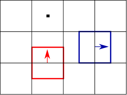
Figure 4: Staggered discretization

For the numerical investigation all model equations are implemented in DuMu^x[KOCH2021423] , using Newton’s method as a nonlinear solver and backward Euler for temporal discretization in transient problems. The equations are discretized in space with the finite volume method on a regular rectangular grid, using Dune-SPGrid [nolte2011] and an adapted Dune-Subgrid [graeser2009] to model the considered geometries with periodic boundaries. For the phase-field and pressure unknowns a cell-centered approach is used, with control volumes equal to grid cells and degrees of freedom placed at their centers. Fluxes over control-volume faces are approximated using the two adjacent values. For the velocities a staggered discretization is used (see Figure 4), with separate degrees of freedom for each velocity component placed at the edges between grid cells and control volumes centered around them.

While the cell problem for the phase field uses only the cell-centered discretization, the pore-scale problem and the cell problems for velocity contributions require a coupled system of cell-centered pressures and staggered velocities. In DuMu^xthis is achieved using a multidomain formulation with a coupling manager handling the volume coupling of the different discretizations of a shared domain [KOCH2021423]. For the pore-scale model the existing coupling manager for Navier-Stokes models was extended to additionally exchange phase-field data.

For the phase-field equation a boundary condition prescribing the flux implements the contact angle condition. In the velocity problems a no-flux condition for the mass conservation and homogeneous Dirichlet conditions for the normal velocity are used at the fluid-solid interfaces. To implement Navier slip boundary conditions a solution-dependent flux can be described. In the case of the cell problem capturing surface tension effects the additional flux can be given based on the prescribed contact angle. On the outer boundary of the reference cell $Y$ periodicity conditions are prescribed.

4.2 Pore-scale simulation

We present an examplary simulation of the fully coupled and non-dimensionalized pore-scale model from Section 3.1. In a channel geometry containing both phases the system conforms to a prescribed contact angle and the interface is advected by a pressure gradient. This could be applied to simulating two-phase flow through a narrowing in a porous medium.

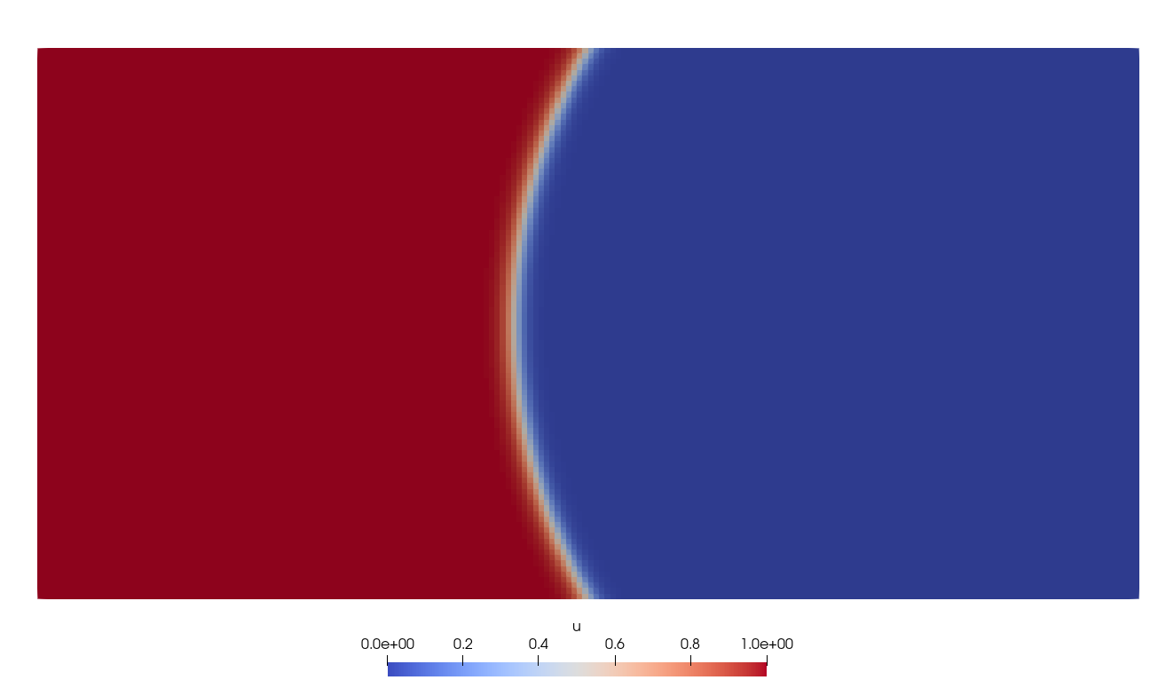
Figure 5: Initial condition of pore-scale simulation of two-phase flow through a channel. $u=1$ (red) corresponds to fluid 1, $u=0$ (blue) to fluid 2.

We consider a two-dimensional domain $\Omega=(0,0.2)\times(0,0.1)$. At the inlet ($x=0$) and outlet ($x=0.2$) we prescribe fixed pressures and fluxes for the phase-field equation. The top and bottom boundaries are walls with slip boundary conditions for the velocity and no-flux boundary conditions for the density. For the phase field we apply the contact angle boundary condition (16) with contact angle $\theta_{\mathrm{eq}}=\pi/3$.

We initialize the fluid distribution with fluid 1 on the left and fluid 2 on the right with a curved and diffuse interface between them, see Figure 5. We prescribe a non-dimensional slip length of 0.01 and a surface tension of $10^{-6}\mathrm{m^{2}}$. The simulation was run for constant fluid properties, using a density of $10^{2}\mathrm{kg/m^{3}}$ and dynamic viscosity of $10^{-2}\mathrm{kg/(m\cdot s)}$. Applying a pressure drop of $450\mathrm{kg/(m\cdot s^{2})}$ leads to a maximum flow velocity of $5.7\cdot 10^{-4}\mathrm{m/s}$.

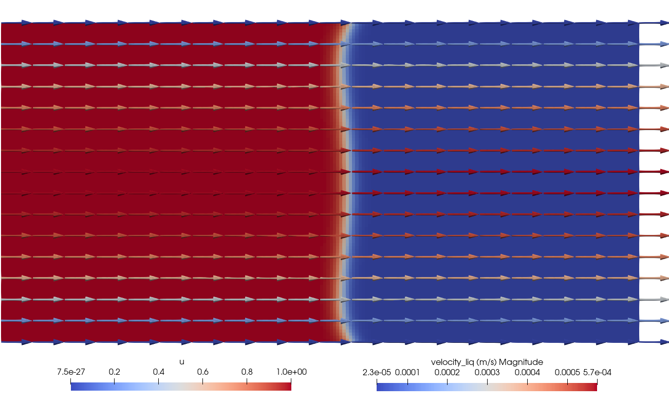
Figure 6: Phase distribution at $t=40\mathrm{s}$ for the pore-scale simulation, overlaid with the velocity field. $u=1$ (red) corresponds to fluid 1, $u=0$ (blue) to fluid 2.

Figure 6 shows the fluid distribution at $t=40\mathrm{s}$. Due to very weak surface tension forces in this setup, the velocity field does not deviate significantly from a parabolic flow profile. In the center of the channel the interface is advected by these higher velocities, leading to an inversion of the curvature. At the three-phase contact point the prescribed contact angle is successfully maintained despite the near-parabolic profile.

4.3 Cell problems

We consider the cell problems (49) and (50) for the velocity components $\mathbf{w}_{j}$ and investigate the behavior of the resulting effective parameters. The derived two-scale model is similar to two-phase Darcy’s law, with effective parameters computed from cell problems rather than prescribed relative permeability saturation curves. We investigate how the computed parameters compare to commonly used curves and under which conditions core assumptions such as a monotone relation is violated. Anisotropic permeabilities are not the focus of this investigation and we choose simple geometries such that the intrinsic permeability of the pore geometry can be separated from fluid-fluid interactions. This allows us to isolate the influence of the fluid distribution on the relative permeability in a simple manner.

For two different geometries we vary the local phase field to determine the effects of saturation and phase distribution and the impact of the dimensionless ratios for viscosity and density as well as the surface tension. Both the slip length and the contact angle influence the results, see e.g. the investigation of dynamic contact angles in [lunowa2021], but will not be considered here. Instead these effects will be controlled by a no-slip condition for the velocity components and a homogeneous neumann condition for the phase field, encoding a neutral contact angle. Since our goal is to address behavior of the effective parameters, we do not couple the flow to the cell problem for the phase distribution (48). Instead we manually prescribe a phase-field function corresponding to a certain saturation and run a few timesteps of the instationary version of the phase-field equation (48) without advection in order to enforce the neutral contact angle. This fluid distribution is then used to solve (49) and (50).

The two domains under consideration vary in geometry and porosity, see Figure 7. The first setup, ”obstacle”, contains a square of side length $0.45$ placed in the center of the domain, leaving a void fraction of $79.75\%$. The second investigated geometry, denoted ”cross”, is a cross of channels with diameter $0.3$, resulting in a porosity of $51\%$.

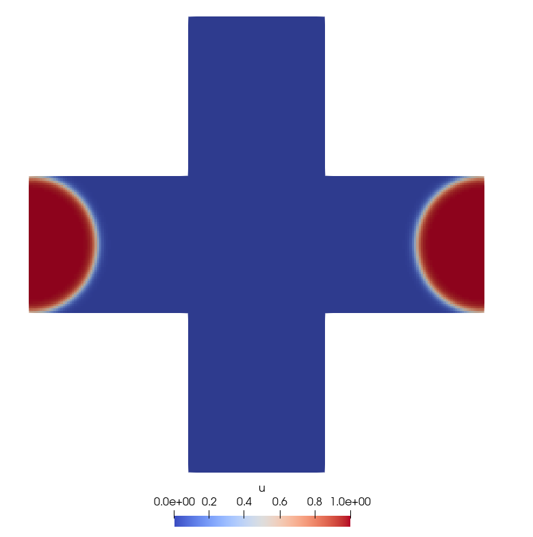
Figure 7: Investigated cell geometries ”obstacle” and ”cross”. $u=1$ (red) corresponds to fluid 1, $u=0$ (blue) to fluid 2.

We consider four core scenarios of which the first three investigate the effective mobility $\mathcal{K}^{(k)}$ for different ratios of viscosity $M$ and density $R$. In the last setup the surface tension tensor $\mathcal{M}^{(k)}$ is analyzed, with identical fluid properties for both fluids. The dimensionless numbers in the cell problems are chosen as 1.

For all four cases we fix the center of a circle with varying radius $r$ and assign cells inside this circle to phase 1, with the rest of the void space being filled with fluid 2. This initial data already contains a diffuse interface according to the following radial function.

$$u(r)=\frac{1}{1+\exp(5/\xi\cdot r)}~{}.$$ (51)

This initial data is evolved under the transient version of the Allen-Cahn equation (48) without advection to enforce a neutral contact angle (see Figure 8). The resulting phase field is fed into the different cell problems for flow velocity components (49), (50), which are then solved.

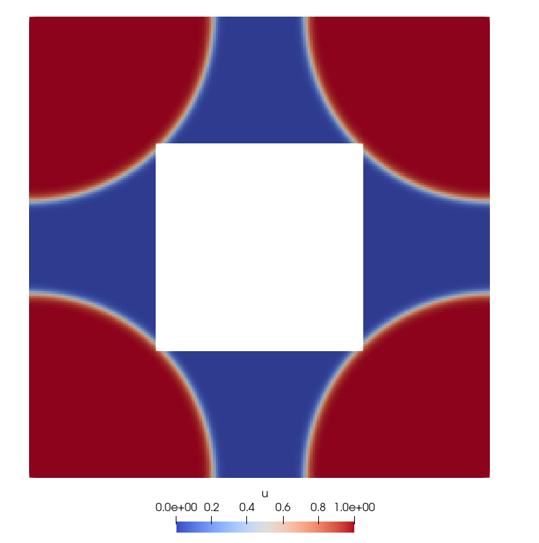
Figure 8: Preprocessing to enforce a neutral contact angle. Initial condition from (51) (left), and the resulting phase field with desired contact angle (right).

In the ”cross” cell geometry we observe recirculation patterns (Figure 14), and e.g. for a horizontal pressure gradient forcing flow from left to right the recirculation near the top and bottom of the domain leads to flow from right to left at these edges of the periodic cell. Depending on the fluid distribution one of the phases may contain primarily these flows in the opposite direction to the main flow, leading to negative integrated velocities. As the effective mobility should capture net flow through the cell, we exclude these recirculations based on the computed flow field, avoiding negative mobilities. The computed velocity field is loaded into ParaView [paraview], computing streamlines from the boundaries and marking affected cells. This process is not performed for the flow problem driven by surface tension (50).

After postprocessing we compute the weighted integrals over marked cells to obtain the effective parameters. The saturation and an approximation to the specific interfacial area are determined by integrals over the entire domain.

$$S^{(1)}=\frac{1}{|\mathcal{P}|}\int_{\mathcal{P}}u_{0}\,\mathrm{d}\mathbf{y}\,,\quad A=\frac{1}{|\mathcal{P}|}\int_{\mathcal{P}}\frac{4}{\xi}u_{0}(1-u_{0})\,\mathrm{d}\mathbf{y}$$ (52)

For the effective mobility $\mathcal{K}^{(k)}$, the computed entries are divided by the absolute permeability and multiplied with the viscosity, yielding a relative permeability. The results are plotted over the saturation of phase 1.

4.3.1 Equal fluid properties

In the first case we consider two fluids with equal viscosity and density ($M=R=1$). The cell problems for velocity contributions driven by the global pressure gradient treat the two-phase system as single-phase flow. The effective mobilities are obtained through integration weighted by the phase-indicator $u^{(k)}$ and the resulting relative permeabilities always sum to 1, see Figure 9.

Due to the symmetries in the fluid distribution the relative permeability is approximately a diagonal matrix and we show only the dominant diagonal entries. For the isotropic setup in the ”obstacle” geometry the entries are equal and the relative permability reduces to a scalar value.

Due to the choice of fluid distribution for every radius $r$ the domain corresponding to fluid 1 contains that for lower radii $r^{\prime}<r$ and thus lower saturation. Equivalently, for phase-field functions $u_{1}<u_{2}$ the corresponding saturations fulfil $S_{1}<S_{2}$. Under this condition the relative permeability is monotone with respect to the saturation. For differing fluid distributions this monotonicity is not guaranteed and a higher saturation concentrated at areas of lower velocities can result in a lower permeability. Figure 10 shows changing relative permeabilities for fixed saturation and varying fluid distributions obtained by changing the center of the initial circular subdomain for fluid 1. This information about local phase distribution and its impact on macroscopic flow can only be captured by solving the cell problems.

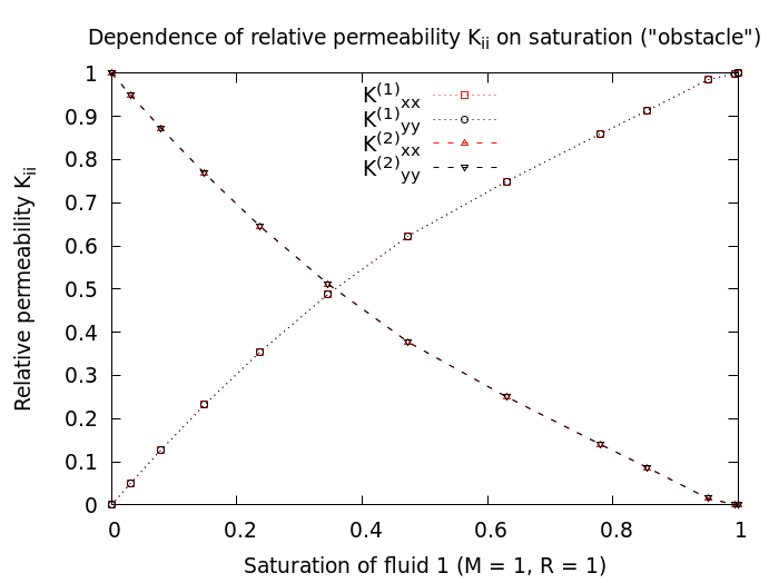
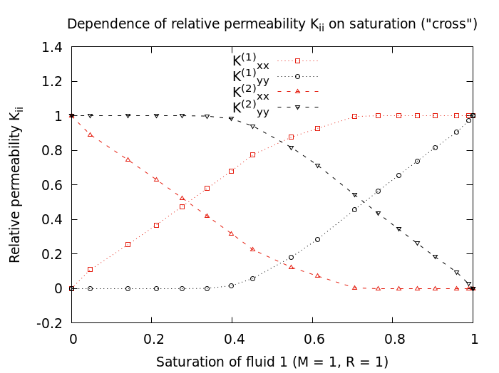
Figure 9: Relative-permeability-saturation relation for equal fluid properties.

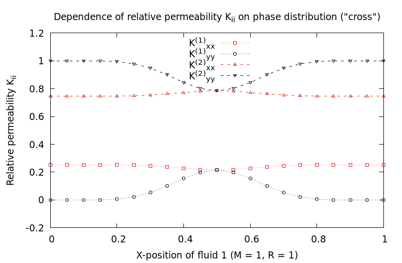
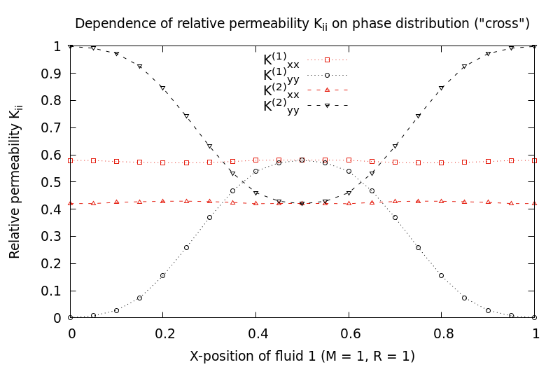
Figure 10: Impact of phase distribution on relative permeability for equal fluid properties with radius $r=0.15$ (left) and $r=0.3$ (right).

4.3.2 Influence of viscosity differences

Next we investigate the effect of the viscosity ratio by considering $M=2$, the investigated cell problems now correspond to an incompressible fluid with varying viscosity.

In stark contrast to typically used relative permeability curves we observe non-monotone behavior for the case ”obstacle” with relative permeabilities of the more viscous fluid reaching values above 1 for saturations above 0.8, up to $\mathcal{K}^{(1)}_{xx}=1.039$ at a saturation of 0.95 (see Figure 11). Due to the chosen fluid distribution the less viscous fluid 2 is located on the surface of the solid matrix at low saturations (high saturation for phase 1). This reduces the resistance exerted on the first fluid and results in higher velocities, especially for higher viscosity ratios $M$. Such lubricating effects have been observed experimentally in different settings [berg2008].

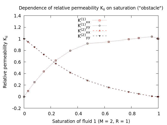
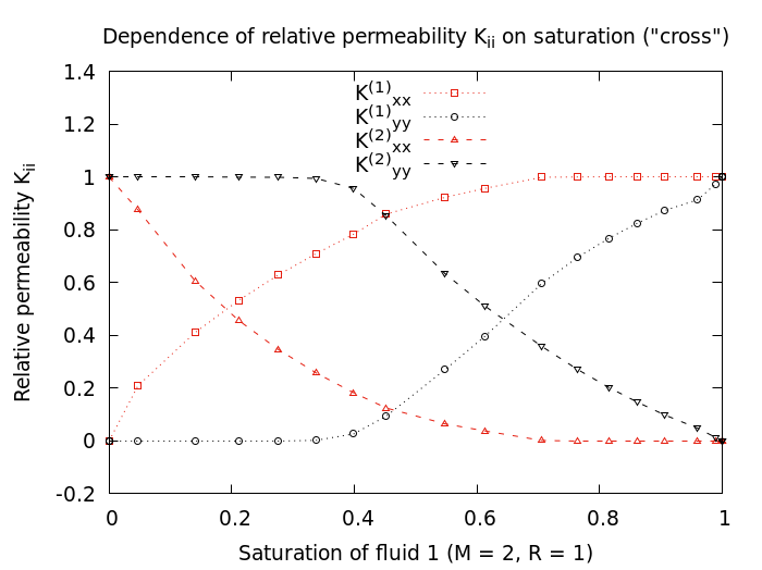
Figure 11: Relative-permeability-saturation relation for viscosity ratio $M=2$.

4.3.3 Influence of density differences

In the case of non-trivial density ratio $R$, the cell problem (49) corresponds to Stokes equation for a quasi-compressible fluid. For ratio $R=2$ (Figure 12) no non-monotone behavior is observed but the curves are notably different to the one obtained for the case of equal fluid properties. For density ratio $R=10$ (Figure 13) non-monotonicity is observed for a horizontal pressure gradient in the ”cross” setup, with the velocity in the lighter fluid increasing as the main flow path is filled with the more dense fluid. The fluid distribution and computed flow field for highest permeability at a saturation of 0.45 are shown in Figure 14. In Figure 15 the results for the ”obstacle” geometry are compared to those for equal fluid properties, which highlights the fact that the sum of the relative permeabilities is less than one.

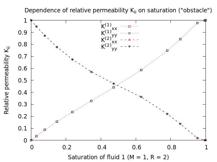
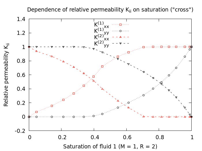
Figure 12: Relative-permeability-saturation relation for density ratio $R=2$.

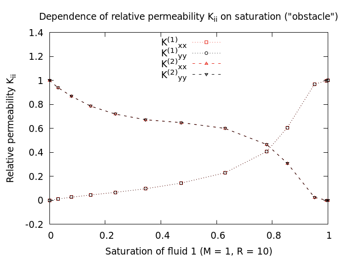
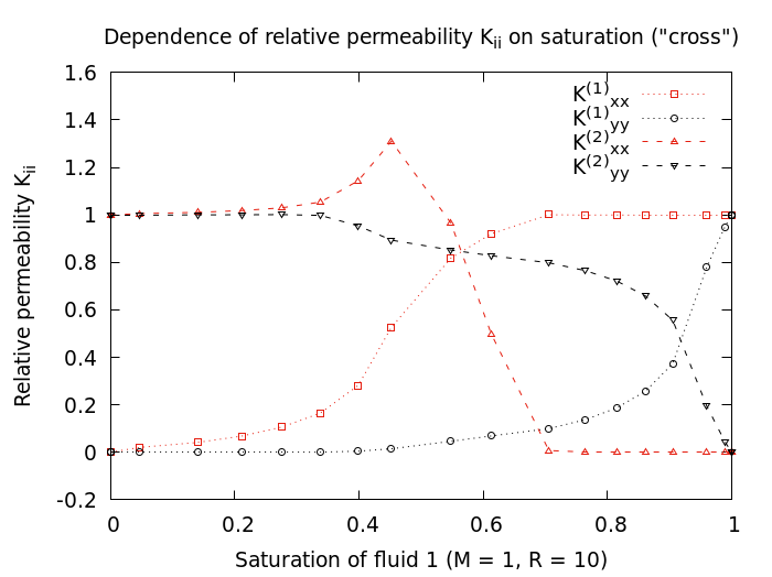
Figure 13: Relative-permeability-saturation relation for density ratio $R=10$.

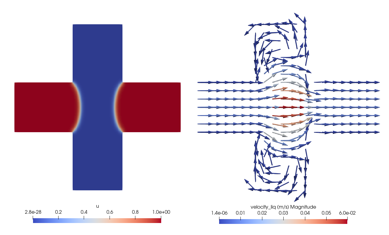
Figure 14: Phase distribution and velocity component for density ratio $R=10$.

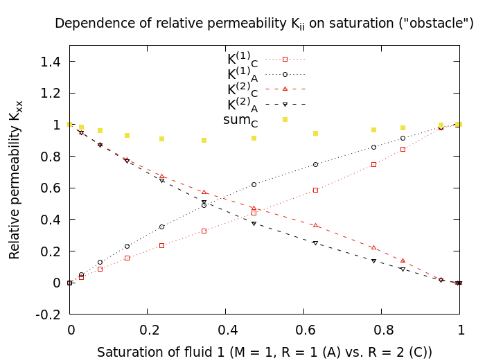
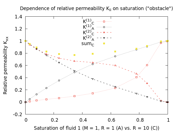
Figure 15: Comparison of relative permeability saturation relation for ”obstacle” geometry.

4.3.4 Surface tension tensor

For the isotropic geometry and fluid distribution considered above the velocities driven by surface tension cancel out in the integral and the computed effective parameter is equal to 0 (Figure 16, left). For asymmetric fluid distributions (Figure 16, right) a non-zero contribution is obtained, but no visible trends are observed as the saturation changes. The redistribution of fluids driven by surface tension forces leads to a net flow for the two phases, which corresponds to $\mathcal{M}^{(k)}$ being non-zero. The size and direction of this net flow and hence the size and sign of the effective parameter $\mathcal{M}^{(k)}$ depends highly on the fluid distribution. Such effects can only be accounted for by solving the cell problem (50).

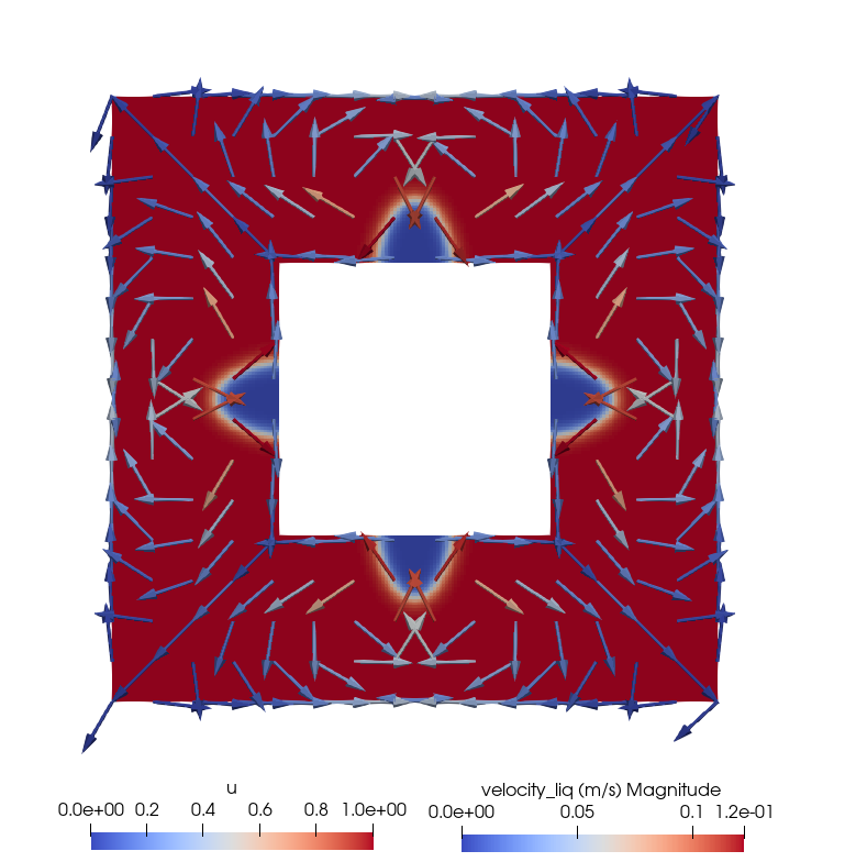
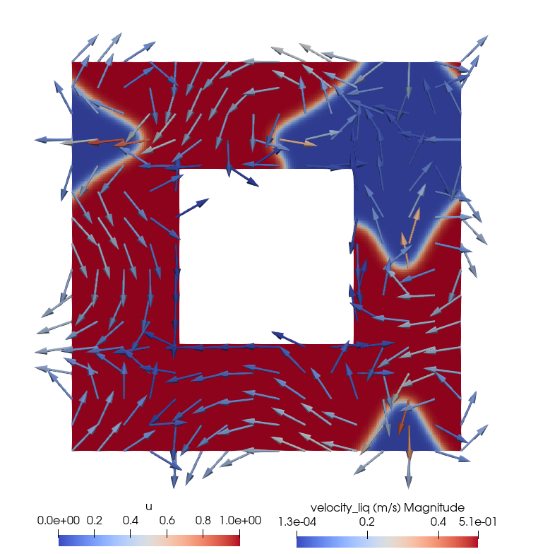
Figure 16: Symmetric and asymmetric case with center at (0.35, 0.3).

4.4 Discussion

For equal fluid properties and fixed fluid distributions we obtain monotone relative permeability saturation curves comparable to commonly used relations such as Brooks-Corey [brooks1966] or van Genuchten [vangenuchten1980]. However, even in this simple case the relative permeability depends not only on saturation but also on the distribution of the fluids. As observed in Section 4.3, even in this simple case no relation can be given without accounting for the local distribution of the fluids.

For differing viscosities the model is able to reproduce non-monotone relative permeabilities with values above 1 as discussed in [berg2008]. When the less viscous fluid coats the solid surface it can reduce the resistance exerted on the more viscous fluid, resulting in higher velocities. Due to the different fluid distribution such a coating is not observed to the same extent for the ”cross” setup, leading to monotone relations for the relative permeability. These effects depend strongly on the local phase distribution and cannot be captured solely by the saturation without additional assumptions.

For moderate density differences the combined permeability is reduced and for higher density ratios non-monotone behavior can be observed. We remark that for very high differences in fluid properties, this should be considered in the derivation of the cell problems and the two-scale problem, which would lead to a different appearance of the effective equations. To obtain equations similar to the often used two-phase Darcy’s law, we use the assumptions presented in Section 3.2.

The derived two-scale model contains an additional effective parameter which accounts for the influence of surface tension between the fluid phases. This is not a common part of the extended Darcy’s law and there is no counterpart to compare it to. A similar cell problem and resulting effective parameter has been investigated by [sharmin2022], incorporating the influence of solute-dependent surface tension. Here only constant surface tension is considered. For symmetric distributions the effective parameter capturing surface tension effects disappears as expected. For anisotropic phase distributions the flow driven by surface tension does not cancel out and the associated cell problem is able to capture significant contributions to effective flow behavior. The size and direction of flow resulting from surface tension and thus the magnitude and sign of the effective parameter depend strongly on the local distribution of fluids.

The numeric investigation of the effective parameters highlights how different fluid distributions with equal saturation can result in very different net flow and effective behavior. Increased relative permeability due to viscosity differences and significant surface tension effects further emphasize the importance of resolving the local fluid morphology.

5 Conclusion

We derived a two-scale model for two-phase flow in porous media using homogenization and investigated the dependence of effective parameters on the fluid distribution in the pore-scale cell problems.

The model consists of macro-scale equations similar to the extended Darcy’s law with effective parameters computed from solutions to cell problems defined at every macroscopic point. One of the effective parameters can be understood as an effective mobility, while the second effective parameter represents effects of interfacial tension on the effective flow. On the pore-scale the phase distribution is captured by a phase field, using an advective Allen-Cahn formulation. For the velocity field we use a stationary Stokes equation with phase-dependent fluid properties and an additional source term incorporating surface tension forces.

The two-scale structure allows to investigate numerically the effects of pore-scale information on effective behavior. We construct local fluid distributions for the pore scale and solve the cell problems associated with pressure driven velocity contributions.

The similarity to two-phase Darcy’s law motivates a comparison of the dependence of relative permeabilities on saturation. By selecting isotropic pore geometries, relative permeability tensors can be extracted from the effective parameters $\mathcal{K}^{(k)}$ in our model and for isotropic fluid distributions these simplify to diagonal matrices or scalar values. As one of the core qualities of relative-permability-saturation-curves we investigate the conditions under which a monotone relationship is obtained. If a common fluid morphology is maintained for different saturations, then for equal fluid properties monotone curves, similar to commonly used functions like van Genuchten and Brooks-Corey, are obtained. The calculated curves however depend strongly on the fluid distribution and change with the pore geometry, highlighting the need to account for pore-scale information. For different viscosities the model can produce non-monotone relationships and relative permeabilities greater than 1. This can be related to a lubricating effect of the less viscous fluid coating the surface of the solid matrix, an effect observed experimentally. For moderate density ratios the effective total permeability decreases and no non-monotone behavior was observed.

We also performed numeric simulations for the cell problem corresponding to the effective parameter $\mathcal{M}^{(k)}$, capturing effects of surface tension forces. For isotropic geometry and fluid morphologies these forces result in no net flow and a vanishing effective parameter. For asymmetric fluid distributions we obtain significant net flows captured by $\mathcal{M}^{(k)}$.

Our two-scale model for two-phase flow captures pore-scale fluid-fluid interactions related to surface tension forces as well as differences in viscosity and density. Through numeric investigation of the effective parameters we highlight the importance of local fluid distribution for accurately capturing effective flow behavior.

Acknowledgments

Funded by Deutsche Forschungsgemeinschaft (DFG, German Research Foundation) under Germany’s Excellence Strategy - EXC 2075 - 390740016. We acknowledge the support by the Stuttgart Center for Simulation Science (SimTech). We thank the Deutsche Forschungsgemeinschaft (DFG, German Research Foundation) for supporting this work by funding SFB 1313, Project Number 327154368.

The authors would like to thank Kundan Kumar (University of Bergen) for useful discussions on monotonicity of relative permeability saturation curves.

Appendix A Sharp-interface limit

In the limit $\xi\to 0$ the phase-field model presented in Section 2.2 recovers the sharp-interface model from Section 2.1. Following the approach of matched asymptotic expansions [caginalp1988] we consider the behavior at the transition zone and in the bulk phases separately, connecting them with matching conditions. Let $L$ be a reference length and ${\bar{\xi}}=\xi/L$ the non-dimensional interface width.

We assume asymptotic expansions in ${\bar{\xi}}$ that capture the behavior away from the interface (outer expansions) for unknowns $\psi\in\{u,p,\mathbf{v}\}$

$$\psi^{\mathrm{out}}(t,\mathbf{x})=\sum_{k=0}^{\infty}{\bar{\xi}}^{k}\psi^{\mathrm{out}}_{k}(t,\mathbf{x})~{}.$$ (53)

For inner expansions at the diffuse interface we consider local curvilinear coordinates. Let $\Gamma_{\bar{\xi}}(t)=\{\mathbf{y}_{\bar{\xi}}\in\mathcal{P}\mid u(t,\mathbf{y}_{\bar{\xi}})=1/2\}$ be the reconstructed interface. With a parametrization $\mathbf{s}$ along $\Gamma_{\bar{\xi}}(t)$ and normal $\mathbf{n}_{\bar{\xi}}(t,\mathbf{s})$ pointing into fluid 2, we define a signed distance $r$ for points near the interface, such that

$$\mathbf{x}=\mathbf{y}_{\bar{\xi}}(t,\mathbf{s})+r\mathbf{n}_{\bar{\xi}}(t,\mathbf{s})~{}.$$ (54)

Note than $\partial_{t}r=-v_{n}$, with $v_{n}$ the velocity of the interface in direction of $\mathbf{n}_{\bar{\xi}}$ corresponding to the sharp-interface velocity $V_{\Gamma_{f}}$. Furthermore it can be shown (see [caginalp1988]) that for mean and Gaussian interface curvatures $\kappa$ and $\Pi$

$$|\nabla r|=1,\quad\nabla r\cdot\nabla s_{i}=0,\quad\nabla^{2}r=\frac{\kappa+2\Pi r}{1+\kappa r+\Pi r^{2}}~{}.$$

The outer expansions define the interface $\Gamma^{\mathrm{out}}_{0}(t)=\{\mathbf{x}\in\mathcal{P}\mid u^{\mathrm{out}}_{0}(t,\mathbf{x})=1/2\}$ with normal vector $\mathbf{n}_{0}$, interfacial velocity $v_{n,0}$ and mean curvature $\kappa_{0}$. The point $\mathbf{y}_{\bar{\xi}}$ can be expressed through expansions

$$\mathbf{y}_{\bar{\xi}}=\sum_{k=0}^{\infty}{\bar{\xi}}^{k}\mathbf{y}_{k}$$

with $\mathbf{y}_{0}\in\Gamma^{\mathrm{out}}_{0}(t)$, and similarly $\mathbf{n}_{\bar{\xi}}=\mathbf{n}_{0}+{\bar{\xi}}\mathbf{n}_{1}+\mathcal{O}({\bar{\xi}}^{2})$. Defining $z=r/{\bar{\xi}}$, we consider the inner expansions in the variables $z$ and $\mathbf{s}$

$$\psi^{\mathrm{in}}(t,\mathbf{x})=\sum_{k=0}^{\infty}{\bar{\xi}}^{k}\psi^{\mathrm{in}}_{k}(t,z,\mathbf{s})~{}.$$ (55)

The derivatives are rewritten accordingly, yielding [caginalp1988]

$$\partial_{t}\psi =-{\bar{\xi}}^{-1}v_{n,0}\partial_{z}\psi^{\mathrm{in}}+(\partial_{t}+\partial_{t}\mathbf{s}\cdot\nabla_{\mathbf{s}})\psi^{\mathrm{in}}+\mathcal{O}({\bar{\xi}})~{},$$ (56)

$$\nabla_{\mathbf{x}}\psi ={\bar{\xi}}^{-1}\partial_{z}\psi^{\mathrm{in}}\mathbf{n}_{0}+\nabla_{\Gamma}\psi^{\mathrm{in}}+\mathcal{O}({\bar{\xi}})~{},$$

$$\nabla_{\mathbf{x}}\cdot\mathbf{\psi} ={\bar{\xi}}^{-1}\partial_{z}\mathbf{\psi}^{\mathrm{in}}\cdot\mathbf{n}_{0}+\nabla_{\Gamma}\cdot\mathbf{\psi}^{\mathrm{in}}+\mathcal{O}({\bar{\xi}})~{},$$

$$\nabla_{\mathbf{x}}^{2}\psi ={\bar{\xi}}^{-2}\partial_{zz}\psi^{\mathrm{in}}+{\bar{\xi}}^{-1}\kappa_{0}\partial_{z}\psi^{\mathrm{in}}+\mathcal{O}(1)~{},$$

using the expansions $v_{n}=v_{n,0}+\mathcal{O}({\bar{\xi}})$ and $\kappa=\kappa_{0}+\mathcal{O}({\bar{\xi}})$. For fixed $t$ and $\mathbf{s}$, let $\mathbf{y}_{1/2\pm}$ denote the limit for $r\searrow 0$ and $r\nearrow 0$ respectively of a point $\mathbf{y}$ in curvilinear coordinates (54). The values of outer expansions at $\mathbf{y}_{1/2\pm}$ are paired with the limit values of inner expansions for $z\to\pm\infty$ in the following matching conditions.

$$\lim_{z\to\pm\infty}\psi^{\mathrm{in}}_{0}(t,z,\mathbf{s}) =\psi^{\mathrm{out}}_{0}(t,\mathbf{y}_{1/2\pm})~{},$$ (57)

$$\lim_{z\to\pm\infty}\partial_{z}\psi^{\mathrm{in}}_{0}(t,z,\mathbf{s}) =0~{},$$

$$\lim_{z\to\pm\infty}(\psi^{\mathrm{in}}_{0}(t,z,\mathbf{s})-(z+y_{1})\nabla\psi^{\mathrm{out}}_{0}(t,\mathbf{y}_{1/2\pm})\cdot\mathbf{n}_{0}) =\psi^{\mathrm{out}}_{1}(t,\mathbf{y}_{1/2\pm})~{},$$

$$\lim_{z\to\pm\infty}\partial_{z}\psi^{\mathrm{in}}_{1}(t,z,\mathbf{s}) =\nabla\psi^{\mathrm{out}}_{0}(t,\mathbf{y}_{1/2\pm})\cdot\mathbf{n}_{0}~{}.$$

A.1 Outer expansions

Due to the polynomial structure of $P^{\prime}$ it can be expanded as

$$P^{\prime}(u_{0}+{\bar{\xi}}u_{1}+\mathcal{O}({\bar{\xi}}^{2}))=P^{\prime}(u_{0})+{\bar{\xi}}u_{1}P^{\prime\prime}(u_{0})+\mathcal{O}({\bar{\xi}}^{2})~{}.$$ (58)

Substituting the outer expansions (53) into the phase-field equation (8) yields

$$0 =L^{2}{\bar{\xi}}^{2}\frac{\partial}{\partial t}(u^{\mathrm{out}}_{0}+\mathcal{O}({\bar{\xi}}^{1}))+L^{2}{\bar{\xi}}^{2}\nabla\cdot((\mathbf{v}_{0}+\mathcal{O}({\bar{\xi}}^{1}))(u^{\mathrm{out}}_{0}+\mathcal{O}({\bar{\xi}}^{1})))$$

$$-\sigma L^{3}{\bar{\xi}}^{2}\nabla^{2}(u^{\mathrm{out}}_{0}+\mathcal{O}({\bar{\xi}}^{1}))+\sigma L{\bar{\xi}}P^{\prime}(u^{\mathrm{out}}_{0}+{\bar{\xi}}u^{\mathrm{out}}_{1}+\mathcal{O}({\bar{\xi}}^{2}))$$ (59a)

$$=\big{[}\sigma L{\bar{\xi}}P^{\prime}(u^{\mathrm{out}}_{0})\big{]}+\mathcal{O}({\bar{\xi}}^{2})~{}.$$ (59b)

The leading order equation $P^{\prime}(u^{\mathrm{out}}_{0})=0$ has solutions $u^{\mathrm{out}}_{0}\in\{0,1/2,1\}$, of which 0 and 1 are stable minimizers of $P$. This allows a decomposition of the unified $\mathcal{P}$ into bulk domains $\Omega^{\mathrm{out}}_{1}$ and $\Omega^{\mathrm{out}}_{2}$ for fluid 1 and 2, respectively, through

$$\Omega^{\mathrm{out}}_{1}(t):=\{\mathbf{x}\in\mathcal{P}\mid u^{\mathrm{out}}_{0}(t,\mathbf{x})=1\}~{},\qquad\Omega^{\mathrm{out}}_{2}(t):=\{\mathbf{x}\in\mathcal{P}\mid u^{\mathrm{out}}_{0}(t,\mathbf{x})=0\}~{}.$$ (60)

We consider the remaining outer expansions for $\Omega^{\mathrm{out}}_{i}$.

For the mass balance equation (6a) we obtain by using the linear dependence of density on the phase-field variable

$$0= \frac{\partial}{\partial t}(\rho(u^{\mathrm{out}}_{0})+\mathcal{O}({\bar{\xi}}))+\nabla\cdot((\rho(u^{\mathrm{out}}_{0})+\mathcal{O}({\bar{\xi}}))(\mathbf{v}^{\mathrm{out}}_{0}+\mathcal{O}({\bar{\xi}})))$$ (61a)

$$= \frac{\partial\rho_{i}}{\partial t}+\nabla\cdot(\rho_{i}\mathbf{v}^{\mathrm{out}}_{0})+\mathcal{O}({\bar{\xi}})~{}.$$ (61b)

Denoting phase velocities $\mathbf{v}_{i}={\mathbf{v}^{\mathrm{out}}_{0}}|_{\Omega^{\mathrm{out}}_{i}}$ we recover the individual mass conservation equations and, due to constant phase densities $\rho_{i}$, the divergence-free condition (1). The momentum balance (6b) yields, using additionally the linear relation for viscosity,

$$0= \frac{\partial}{\partial t}((\rho(u^{\mathrm{out}}_{0})+\mathcal{O}({\bar{\xi}}))(\mathbf{v}^{\mathrm{out}}_{0}+\mathcal{O}({\bar{\xi}})))$$

$$+\nabla\cdot((\rho(u^{\mathrm{out}}_{0})+\mathcal{O}({\bar{\xi}}))(\mathbf{v}^{\mathrm{out}}_{0}+\mathcal{O}({\bar{\xi}}))\otimes(\mathbf{v}^{\mathrm{out}}_{0}+\mathcal{O}({\bar{\xi}})))$$

$$+\nabla(p^{\mathrm{out}}_{0}+\mathcal{O}({\bar{\xi}}))$$

$$-\nabla\cdot\bigg{(}(\mu(u^{\mathrm{out}}_{0})+\mathcal{O}({\bar{\xi}}))\bigg{(}\nabla(\mathbf{v}^{\mathrm{out}}_{0}+\mathcal{O}({\bar{\xi}}))+(\nabla(\mathbf{v}^{\mathrm{out}}_{0}+\mathcal{O}({\bar{\xi}})))^{T}$$

$$-\frac{2}{3}(\nabla\cdot(\mathbf{v}^{\mathrm{out}}_{0}+\mathcal{O}({\bar{\xi}})))\mathbf{I}\bigg{)}\bigg{)}$$

$$-(\rho(u^{\mathrm{out}}_{0})+\mathcal{O}({\bar{\xi}}))\mathbf{g}+\mathcal{O}({\bar{\xi}})$$ (62a)

$$= \frac{\partial}{\partial t}(\rho_{i}\mathbf{v}_{i})+\nabla\cdot(\rho_{i}\mathbf{v}_{i}\otimes\mathbf{v}_{i})+\nabla p^{\mathrm{out}}_{0}$$

$$-\nabla\cdot\bigg{(}\mu_{i}\bigg{(}\nabla\mathbf{v}_{i}+(\nabla\mathbf{v}_{i})^{T}-\frac{2}{3}(\nabla\cdot\mathbf{v}_{i})\mathbf{I}\bigg{)}\bigg{)}-\rho_{i}\mathbf{g}+\mathcal{O}({\bar{\xi}})$$ (62b)

With phase pressures $p_{i}$ given by restricting $p^{\mathrm{out}}_{0}$ to the bulk domain $\Omega^{\mathrm{out}}_{i}$ we recover the momentum balance (2).

Inserting the outer expansions into the boundary conditions yields the conditions for the fluid-solid interfaces of the sharp-interface model. From (9a) we obtain

$$0 =(\mathbf{v}^{\mathrm{out}}_{0}+\mathcal{O}({\bar{\xi}}))+\lambda\nabla((\mathbf{v}^{\mathrm{out}}_{0}+\mathcal{O}({\bar{\xi}}))\cdot(\mathbf{t}_{0}+\mathcal{O}({\bar{\xi}})))\cdot(\mathbf{n}_{0}+\mathcal{O}({\bar{\xi}}))(\mathbf{t}_{0}+\mathcal{O}({\bar{\xi}}))$$ (63a)

$$=\mathbf{v}_{i}+\lambda\nabla(\mathbf{v}_{i}\cdot\mathbf{t}_{0})\cdot\mathbf{n}_{0}\,\mathbf{t}_{0}~{},$$ (63b)

corresponding to the slip condition (3).

A.2 Inner expansions

To obtain the boundary conditions at the fluid-fluid interface we insert the inner expansions (55), rewriting derivatives according to (56), and use the matching conditions (57).

Phase-field equation

From the phase-field equation (8) we obtain due to the polynomial form of $P$

$$0= L^{2}{\bar{\xi}}^{2}(-{\bar{\xi}}^{-1}v_{n,0}\partial_{z}(u^{\mathrm{in}}_{0}+\mathcal{O}({\bar{\xi}})))+L^{2}{\bar{\xi}}^{2}(-{\bar{\xi}}^{-1}\partial_{z}((\mathbf{v}^{\mathrm{in}}_{0}+\mathcal{O}({\bar{\xi}}))(u^{\mathrm{in}}_{0}+\mathcal{O}({\bar{\xi}})))\cdot\mathbf{n}_{0})$$

$$-\sigma L^{3}{\bar{\xi}}^{3}({\bar{\xi}}^{-2}\partial_{zz}(u^{\mathrm{in}}_{0}+{\bar{\xi}}u^{\mathrm{in}}_{1}+\mathcal{O}({\bar{\xi}}^{2}))+{\bar{\xi}}^{-1}\kappa_{0}\partial_{z}(u^{\mathrm{in}}_{0}+\mathcal{O}({\bar{\xi}})))$$

$$+\sigma L{\bar{\xi}}(P^{\prime}(u^{\mathrm{in}}_{0})+u^{\mathrm{in}}_{1}P^{\prime\prime}(u^{\mathrm{in}}_{0})+\mathcal{O}({\bar{\xi}}^{2}))$$ (64a)

$$= {\bar{\xi}}\big{[}-\sigma L^{2}\partial_{zz}u^{\mathrm{in}}_{0}+\sigma P^{\prime}(u^{\mathrm{in}}_{0})-L^{2}v_{n,0}\partial_{z}u^{\mathrm{in}}_{0}+L^{2}\partial_{z}(\mathbf{v}^{\mathrm{in}}_{0}u^{\mathrm{in}}_{0})\cdot\mathbf{n}_{0}\big{]}+\mathcal{O}({\bar{\xi}}^{2})~{}.$$ (64b)

Multiplying the leading order terms with $\partial_{z}u^{\mathrm{in}}_{0}$ and integrating with respect to $z$ yields a condition for the interface velocity

$$0= \int_{z=-\infty}^{\infty}\sigma(-L^{3}\partial_{zz}u^{\mathrm{in}}_{0}+LP^{\prime}(u^{\mathrm{in}}_{0}))\partial_{z}u^{\mathrm{in}}_{0}+(-v_{n,0}+\mathbf{v}^{\mathrm{in}}_{0}\cdot\mathbf{n}_{0})L^{2}(\partial_{z}u^{\mathrm{in}}_{0})^{2}\,\mathrm{d}z$$ (65a)

$$= \sigma L^{2}\int_{z=-\infty}^{\infty}-\frac{L}{2}\partial_{z}(\partial_{z}u^{\mathrm{in}}_{0})^{2}+\partial_{z}P(u^{\mathrm{in}}_{0})\,\mathrm{d}z+(-v_{n,0}+\mathbf{v}^{\mathrm{in}}_{0}\cdot\mathbf{n}_{0})L^{2}\int_{z=-\infty}^{\infty}(\partial_{z}u^{\mathrm{in}}_{0})^{2}\,\mathrm{d}z$$ (65b)

$$= \sigma L^{2}\big{[}-\frac{L}{2}(0-0)+(0-0)\big{]}+(-v_{n,0}+\mathbf{v}^{\mathrm{in}}_{0}\cdot\mathbf{n}_{0})\frac{2L}{3}~{},$$ (65c)

where the terms in the first integral are equal to 0 due to the matching conditions. Taking the limit in $z$, we obtain

$$v_{n,0}=\mathbf{v}^{\mathrm{out}}_{0}(t,\mathbf{y}_{1/2\pm})\cdot\mathbf{n}_{0}~{}.$$ (66)

With $\mathbf{v}^{\mathrm{in}}_{0}\cdot\mathbf{n}_{0}$ independent of $z$, the leading order terms reduce to

$$0=-\sigma L^{2}\partial_{zz}u^{\mathrm{in}}_{0}+\sigma P^{\prime}(u^{\mathrm{in}}_{0})~{}.$$ (67)

Multiplying the remaining terms with $\partial_{z}u^{\mathrm{in}}_{0}$ and integrating with respect to $z$ yields, applying the chain rule and matching conditions with $u^{\mathrm{in}}_{0}(t,\mathbf{y}_{1/2-})=0$ and $P(0)=0$,

$$0= \int_{z^{\prime}=-\infty}^{z}-L^{2}\partial_{z}u^{\mathrm{in}}_{0}\partial_{zz}u^{\mathrm{in}}_{0}+\partial_{z}u^{\mathrm{in}}_{0}P^{\prime}(u^{\mathrm{in}}_{0})\,\mathrm{d}z$$ (68a)

$$= \int_{z^{\prime}=-\infty}^{z}-L^{2}\frac{1}{2}\partial_{z}((\partial_{z}u^{\mathrm{in}}_{0})^{2})+\partial_{z}P(u^{\mathrm{in}}_{0})\,\mathrm{d}z$$ (68b)

$$= -L^{2}(\partial_{z}u^{\mathrm{in}}_{0}(t,z,\mathbf{s}))^{2}-0+2P(u^{\mathrm{in}}_{0}(t,z,\mathbf{s}))-0~{}.$$ (68c)

By definition of the curvilinear coordinates we have $\partial_{z}u^{\mathrm{in}}_{0}\geq 0$ and

$$\partial_{z}u^{\mathrm{in}}_{0}=L^{-1}\sqrt{2P(u^{\mathrm{in}}_{0})}~{}.$$ (69)

Using $u^{\mathrm{out}}(t,0,\mathbf{s})=1/2$ one can obtain a profile for the phase-field, namely

$$u^{\mathrm{in}}_{0}(t,z,\mathbf{s})=u^{\mathrm{in}}_{0}(z)=\frac{1}{1+\exp{4z/L}}=\frac{1}{2}\left(1+\tanh\left(\frac{2z}{L}\right)\right)~{}.$$ (70)

Mass balance

Inserting the inner expansions into the mass balance equation (6a) yields

$$0= (-{\bar{\xi}}^{-1}v_{n,0}\partial_{z}+\mathcal{O}(1))(\rho(u^{\mathrm{in}}_{0})+\mathcal{O}({\bar{\xi}}))$$

$$+{\bar{\xi}}^{-1}\partial_{z}((\mathbf{v}^{\mathrm{in}}_{0}+\mathcal{O}({\bar{\xi}}))(\rho(u^{\mathrm{in}}_{0})+\mathcal{O}({\bar{\xi}})))\cdot\mathbf{n}_{0}+\mathcal{O}(1)$$ (71a)

$$= {\bar{\xi}}^{-1}\big{[}-v_{n,0}\partial_{z}\rho(u^{\mathrm{in}}_{0})+\partial_{z}(\mathbf{v}^{\mathrm{in}}_{0}\rho(u^{\mathrm{in}}_{0}))\cdot\mathbf{n}_{0}\big{]}+\mathcal{O}(1)~{}.$$ (71b)

Integrating with respect to $z$ and applying the matching conditions we obtain

$$0= \int_{z=-\infty}^{\infty}-v_{n,0}\partial_{z}\rho(u^{\mathrm{in}}_{0})+\partial_{z}(\mathbf{v}^{\mathrm{in}}_{0}\rho(u^{\mathrm{in}}_{0}))\,\mathrm{d}z$$ (72a)

$$= -v_{n_{0}}(\rho(1)-\rho(0))+(\mathbf{v}^{\mathrm{out}}_{0}(t,\mathbf{y}_{1/2+})\rho(1)-\mathbf{v}^{\mathrm{out}}_{0}(t,\mathbf{y}_{1/2-})\rho(0))$$ (72b)

$$= -v_{n,0}(\rho_{1}-\rho_{2})+(\mathbf{v}_{1}\rho_{1}-\mathbf{v}_{2}\rho_{2})~{},$$ (72c)

which is fulfilled for $v_{1}=v_{2}=v_{n,0}$ at the interface.

Momentum balance

Inserting the inner expansions into the momentum balance equation (6b) yields

$$0= -{\bar{\xi}}^{-1}v_{n,0}\partial_{z}((\rho(u^{\mathrm{in}}_{0})+\mathcal{O}({\bar{\xi}}))(\mathbf{v}^{\mathrm{in}}_{0}+\mathcal{O}({\bar{\xi}})))+\mathcal{O}(1)$$

$$+{\bar{\xi}}^{-1}\partial_{z}((\rho(u^{\mathrm{in}}_{0})+\mathcal{O}({\bar{\xi}}))(\mathbf{v}^{\mathrm{in}}_{0}+\mathcal{O}({\bar{\xi}}))\otimes(\mathbf{v}^{\mathrm{in}}_{0}+\mathcal{O}({\bar{\xi}})))\mathbf{n}_{0}+\mathcal{O}(1)$$

$$+{\bar{\xi}}^{-1}\partial_{z}(p^{\mathrm{in}}_{0}+\mathcal{O}({\bar{\xi}}))\mathbf{n}_{0}+\mathcal{O}(1)$$

$$-{\bar{\xi}}^{-1}\partial_{z}\bigg{(}(\mu(u^{\mathrm{in}}_{0})+{\bar{\xi}}(M-1)u^{\mathrm{in}}_{1}+\mathcal{O}({\bar{\xi}}^{2}))\bigg{(}{\bar{\xi}}^{-1}\partial_{z}(\mathbf{v}^{\mathrm{in}}_{0}+{\bar{\xi}}\mathbf{v}^{\mathrm{in}}_{1}+\mathcal{O}({\bar{\xi}}^{2}))\otimes\mathbf{n}_{0}$$

$$+\nabla_{\Gamma}(\mathbf{v}^{\mathrm{in}}_{0}+\mathcal{O}({\bar{\xi}}))+{\bar{\xi}}^{-1}(\partial_{z}(\mathbf{v}^{\mathrm{in}}_{0}+{\bar{\xi}}\mathbf{v}^{\mathrm{in}}_{1}+\mathcal{O}({\bar{\xi}}^{2}))\otimes\mathbf{n}_{0})^{T}+(\nabla_{\Gamma}(\mathbf{v}^{\mathrm{in}}_{0}+\mathcal{O}({\bar{\xi}})))^{T}$$

$$-{\bar{\xi}}^{-1}\frac{2}{3}\partial_{z}(\mathbf{v}^{\mathrm{in}}_{0}+{\bar{\xi}}\mathbf{v}^{\mathrm{in}}_{1}+\mathcal{O}({\bar{\xi}}^{2}))\cdot\mathbf{n}_{0}\mathbf{I}-\frac{2}{3}\nabla_{\Gamma}\cdot(\mathbf{v}^{\mathrm{in}}_{0}+\mathcal{O}({\bar{\xi}}))\mathbf{I}+\mathcal{O}({\bar{\xi}})\bigg{)}\bigg{)}\mathbf{n}_{0}$$

$$+\nabla_{\Gamma}\cdot\bigg{(}(\mu(u^{\mathrm{in}}_{0})+\mathcal{O}({\bar{\xi}})){\bar{\xi}}^{-1}\bigg{(}\partial_{z}(\mathbf{v}^{\mathrm{in}}_{0}+\mathcal{O}({\bar{\xi}}))\otimes\mathbf{n}_{0}+(\partial_{z}(\mathbf{v}^{\mathrm{in}}_{0}+\mathcal{O}({\bar{\xi}}))\otimes\mathbf{n}_{0})^{T}$$

$$-\frac{2}{3}\partial_{z}(\mathbf{v}^{\mathrm{in}}_{0}+\mathcal{O}({\bar{\xi}}))\cdot\mathbf{n}_{0}\mathbf{I}+\mathcal{O}({\bar{\xi}})\bigg{)}\bigg{)}-(\rho(u^{\mathrm{in}}_{0})+\mathcal{O}({\bar{\xi}}))\mathbf{g}$$

$$-\frac{3\gamma L}{2}{\bar{\xi}}\Big{[}{\bar{\xi}}^{-1}\partial_{z}\Big{(}{\bar{\xi}}^{-1}\partial_{z}(u^{\mathrm{in}}_{0}+{\bar{\xi}}u^{\mathrm{in}}_{1}+\mathcal{O}({\bar{\xi}}^{2}))\mathbf{n}_{0}+\nabla_{\Gamma}(u^{\mathrm{in}}_{0}+\mathcal{O}({\bar{\xi}}))$$

$$\otimes({\bar{\xi}}^{-1}\partial_{z}(u^{\mathrm{in}}_{0}+{\bar{\xi}}u^{\mathrm{in}}_{1}+\mathcal{O}({\bar{\xi}}^{2}))\mathbf{n}_{0}+\nabla_{\Gamma}(u^{\mathrm{in}}_{0}+\mathcal{O}({\bar{\xi}})))\Big{)}\mathbf{n}_{0}$$

$$+\nabla_{\Gamma}\cdot\Big{(}{\bar{\xi}}^{-1}\partial_{z}(u^{\mathrm{in}}_{0}+\mathcal{O}({\bar{\xi}}))\mathbf{n}_{0}\otimes{\bar{\xi}}^{-1}\partial_{z}(u^{\mathrm{in}}_{0}+\mathcal{O}({\bar{\xi}}))\mathbf{n}_{0}\Big{)}+\mathcal{O}(1)\Big{]}$$

$$+\mathcal{O}(1)$$ (73a)

with leading order

$$= {\bar{\xi}}^{-2}\bigg{[}-\partial_{z}(\mu(u^{\mathrm{in}}_{0})(\partial_{z}\mathbf{v}^{\mathrm{in}}_{0}\otimes\mathbf{n}_{0}+(\partial_{z}\mathbf{v}^{\mathrm{in}}_{0}\otimes\mathbf{n}_{0})^{T}-\frac{2}{3}\partial_{z}\mathbf{v}^{\mathrm{in}}_{0}\cdot\mathbf{n}_{0}\mathbf{I}))\mathbf{n}_{0}$$

$$-\frac{3\gamma L}{2}\partial_{z}(\partial_{z}u^{\mathrm{in}}_{0}\mathbf{n}_{0}\otimes\partial_{z}u^{\mathrm{in}}_{0}\mathbf{n}_{0})\mathbf{n}_{0}\bigg{]}$$ (73b)

and second order

$$+{\bar{\xi}}^{-1}\bigg{[}-v_{n,0}\partial_{z}(\rho(u^{\mathrm{in}}_{0})\mathbf{v}^{\mathrm{in}}_{0})+\partial_{z}(\rho(u^{\mathrm{in}}_{0})\mathbf{v}^{\mathrm{in}}_{0}\otimes\mathbf{v}^{\mathrm{in}}_{0})\mathbf{n}_{0}+\partial_{z}p^{\mathrm{in}}_{0}\mathbf{n}_{0}$$

$$-\partial_{z}\bigg{(}\mu(u^{\mathrm{in}}_{0})\bigg{(}\partial_{z}\mathbf{v}^{\mathrm{in}}_{1}\otimes\mathbf{n}_{0}+(\partial_{z}\mathbf{v}^{\mathrm{in}}_{1}\otimes\mathbf{n}_{0})^{T}-\frac{2}{3}\partial_{z}\mathbf{v}^{\mathrm{in}}_{1}\cdot\mathbf{n}_{0}\mathbf{I}$$

$$+\nabla_{\Gamma}\mathbf{v}^{\mathrm{in}}_{0}+(\nabla_{\Gamma}\mathbf{v}^{\mathrm{in}}_{0})^{T}-\frac{2}{3}\nabla_{\Gamma}\cdot\mathbf{v}^{\mathrm{in}}_{0}\mathbf{I}\bigg{)}$$

$$+(M-1)u^{\mathrm{in}}_{1}\bigg{(}\partial_{z}\mathbf{v}^{\mathrm{in}}_{0}\otimes\mathbf{n}_{0}+(\partial_{z}\mathbf{v}^{\mathrm{in}}_{0}\otimes\mathbf{n}_{0})^{T}-\frac{2}{3}\partial_{z}\mathbf{v}^{\mathrm{in}}_{0}\cdot\mathbf{n}_{0}\mathbf{I}\bigg{)}\bigg{)}\mathbf{n}_{0}$$

$$+\nabla_{\Gamma}\cdot\bigg{(}\mu(u^{\mathrm{in}}_{0})\bigg{(}\partial_{z}\mathbf{v}^{\mathrm{in}}_{0}\otimes\mathbf{n}_{0}+(\partial_{z}\mathbf{v}^{\mathrm{in}}_{0}\otimes\mathbf{n}_{0})^{T}-\frac{2}{3}\partial_{z}\mathbf{v}^{\mathrm{in}}_{0}\cdot\mathbf{n}_{0}\mathbf{I}\bigg{)}\bigg{)}$$

$$-\frac{3\gamma L}{2}\Big{[}\partial_{z}\Big{(}\partial_{z}u^{\mathrm{in}}_{0}\mathbf{n}_{0}\otimes(\partial_{z}u^{\mathrm{in}}_{1}\mathbf{n}_{0}+\nabla_{\Gamma}u^{\mathrm{in}}_{0})+(\partial_{z}u^{\mathrm{in}}_{1}\mathbf{n}_{0}+\nabla_{\Gamma}u^{\mathrm{in}}_{0})\otimes\partial_{z}u^{\mathrm{in}}_{0}\mathbf{n}_{0}\Big{)}\mathbf{n}_{0}$$

$$+\nabla_{\Gamma}\cdot\Big{(}\partial_{z}u^{\mathrm{in}}_{0}\mathbf{n}_{0}\otimes\partial_{z}u^{\mathrm{in}}_{0}\mathbf{n}_{0}\Big{)}+\mathcal{O}(1)\Big{]}\bigg{]}+\mathcal{O}(1)~{}.$$ (73c)

Using the definition of the outer product, the leading order terms at $\mathcal{O}({\bar{\xi}}^{-2})$ can be written as

$$0=-\frac{3\gamma L}{2}\partial_{z}(\partial_{z}u^{\mathrm{in}}_{0})^{2}\mathbf{n}_{0}-\partial_{z}(\mu(u^{\mathrm{in}}_{0})\partial_{z}\mathbf{v}^{\mathrm{in}}_{0})-\partial_{z}\Big{(}\mu(u^{\mathrm{in}}_{0})((\partial_{z}\mathbf{v}^{\mathrm{in}}_{0}\cdot\mathbf{n}_{0})-\frac{2}{3}(\partial_{z}\mathbf{v}^{\mathrm{in}}_{0}\cdot\mathbf{n}_{0})\mathbf{I})\Big{)}\mathbf{n}_{0}$$ (74)

Let $\mathbf{t}_{0}$ the tangential vector, with $\mathbf{t}_{0}\cdot\mathbf{n}_{0}=0$. Taking the dot product of the above (74) with $\mathbf{t}_{0}$ yields

$$0=\partial_{z}(\mu(u^{\mathrm{in}}_{0})\partial_{z}\mathbf{v}^{\mathrm{in}}_{0})\cdot\mathbf{t}_{0}~{}.$$ (75)

Integrating with respect to $z$ and using matching conditions, we obtain

$$\mu(u^{\mathrm{in}}_{0})\partial_{z}\mathbf{v}^{\mathrm{in}}_{0}\cdot\mathbf{t}_{0}=\text{\emph{const.}}=0~{}.$$ (76)

Since $\mu\neq 0$ we have $\partial_{z}\mathbf{v}^{\mathrm{in}}_{0}\cdot\mathbf{t}_{0}=0$, corresponding to the sharp-interface boundary condition and together with the assumption $\partial_{z}\mathbf{v}^{\mathrm{in}}_{0}\cdot\mathbf{n}_{0}=0$ the velocity $\mathbf{v}^{\mathrm{in}}_{0}$ is independent of $z$.

Using also the definition of the outer product as well as $\nabla_{\Gamma}\psi\cdot\mathbf{n}_{0}=0$ , $\nabla_{\Gamma}\cdot\mathbf{n}_{0}=\kappa_{0}$ and $\nabla_{\Gamma}u^{\mathrm{in}}_{0}=0$, the second order terms simplify to

$$0= -v_{n,0}\partial_{z}(\rho(u^{\mathrm{in}}_{0})\mathbf{v}^{\mathrm{in}}_{0})+\partial_{z}(\rho(u^{\mathrm{in}}_{0})\mathbf{v}^{\mathrm{in}}_{0}\otimes\mathbf{v}^{\mathrm{in}}_{0})\mathbf{n}_{0}+\partial_{z}p^{\mathrm{in}}_{0}\mathbf{n}_{0}$$

$$-\partial_{z}\bigg{(}\mu(u^{\mathrm{in}}_{0})\bigg{(}\partial_{z}\mathbf{v}^{\mathrm{in}}_{1}\otimes\mathbf{n}_{0}+(\partial_{z}\mathbf{v}^{\mathrm{in}}_{1}\otimes\mathbf{n}_{0})^{T}-\frac{2}{3}\partial_{z}\mathbf{v}^{\mathrm{in}}_{1}\cdot\mathbf{n}_{0}\mathbf{I}+(\nabla_{\Gamma}\mathbf{v}^{\mathrm{in}}_{0})^{T}-\frac{2}{3}\nabla_{\Gamma}\cdot\mathbf{v}^{\mathrm{in}}_{0}\mathbf{I}\bigg{)}\bigg{)}\mathbf{n}_{0}$$

$$-\frac{3\gamma L}{2}\Big{[}\partial_{z}\Big{(}2\partial_{z}u^{\mathrm{in}}_{0}\partial_{z}u^{\mathrm{in}}_{1}\mathbf{n}_{0}\Big{)}+(\partial_{z}u^{\mathrm{in}}_{0})^{2}\kappa_{0}\mathbf{n}_{0}\Big{)}\Big{]}~{}.$$ (77)

Integrating with respect to $z$ and applying the matching conditions yields

$$0= -v_{n,0}[\rho(u^{\mathrm{out}}_{0})\mathbf{v}^{\mathrm{out}}_{0}]+[\rho(u^{\mathrm{out}}_{0})\mathbf{v}^{\mathrm{out}}_{0}\otimes\mathbf{v}^{\mathrm{out}}_{0}]\mathbf{n}_{0}+[p^{\mathrm{out}}_{0}]\mathbf{n}_{0}$$

$$-[\mu(u^{\mathrm{out}}_{0})(\nabla\mathbf{v}^{\mathrm{out}}_{0}+(\nabla\mathbf{v}^{\mathrm{out}}_{0})^{T}-\frac{2}{3}\nabla\cdot\mathbf{v}^{\mathrm{out}}_{0}\mathbf{I})\mathbf{n}_{0}]-\frac{3\gamma L}{2}\kappa_{0}\mathbf{n}_{0}\int_{z=-\infty}^{\infty}(\partial_{z}u^{\mathrm{in}}_{0})^{2}\,\mathrm{d}z~{},$$ (78)

where $[\psi]=\psi_{1}-\psi_{2}$ denotes the jump of $\psi$ across the interface and we used the boundedness of $\nabla_{\Gamma}\mathbf{v}^{\mathrm{in}}_{0}$ as well as $\partial_{z}u^{\mathrm{in}}_{1}$. As the integral evaluates to $2/(3L)$ and the phase velocities are equal to $v_{n,0}$ at the interface, we recover the boundary condition (5).

Appendix B Non-dimensionalization

As described in Section 3.1, in addition to the two length scales $\ell$ and $L$ with $\epsilon=\ell/L$, we define reference values with dimensions

$$[\hat{L}] =\mathrm{m} [\hat{\ell}] =\mathrm{m} [\hat{\xi}] =\mathrm{m} [\hat{t}] =\mathrm{s} [\hat{v}] =\mathrm{\frac{m}{s}}$$

$$[\hat{\rho}] =\mathrm{\frac{kg}{m^{3}}} [\hat{\mu}] =\mathrm{\frac{kg}{m\cdot s}} [\hat{p}] =\mathrm{\frac{kg}{ms^{2}}} [\hat{}\lambda] =\mathrm{m} [\hat{}\sigma] =\mathrm{\frac{m}{s}}~{},$$

and let

$$\hat{L} =L \hat{\ell} =\ell \hat{\xi} =\hat{\ell} \hat{t} =\frac{L}{\hat{v}} \hat{\rho} =\rho_{2} \hat{\mu} =\mu_{2} \hat{}\lambda =\ell \hat{}\sigma =\sigma~{}.$$

This defines non-dimensionalized variables

$$\bar{\xi} =\frac{\xi}{\hat{\ell}} \bar{}\mathbf{v} =\frac{\mathbf{v}}{\hat{v}} \bar{\rho} =\frac{\rho}{\hat{\rho}} \bar{\mu} =\frac{\mu}{\hat{\mu}} \bar{p} =\frac{p}{\hat{p}} \bar{t} =\frac{t}{\hat{t}} \bar{}\lambda =\frac{\lambda}{\hat{}\lambda}~{},$$

and dimensionless numbers

$$\mathrm{Re}\, =\frac{\hat{\rho}\hat{v}\hat{L}}{\hat{\mu}} \mathrm{Ca}\, =\frac{\hat{v}\hat{\mu}}{\gamma} \mathrm{Eu} =\frac{\hat{p}}{\hat{\rho}\hat{v}^{2}} \mathrm{Fr} =\frac{\hat{v}}{\sqrt{g\hat{L}}} S =\frac{\hat{}\sigma}{\hat{v}}~{}.$$

Inserting into the mass (6a) and momentum (6b) balances yields

$$\frac{\hat{\rho}}{\hat{t}}\frac{\partial\bar{\rho}}{\partial\bar{t}}+\frac{\hat{\rho}\hat{v}}{\hat{L}}\bar{\nabla}\cdot(\bar{\rho}\bar{}\mathbf{v})= 0~{},$$ (79a)

$$\frac{\hat{\rho}\hat{v}}{\hat{t}}\frac{\partial}{\partial\bar{t}}(\bar{\rho}\bar{}\mathbf{v})+\frac{\hat{\rho}\hat{v}^{2}}{\hat{L}}\bar{\nabla}\cdot(\bar{\rho}\bar{}\mathbf{v}\otimes\bar{}\mathbf{v})= -\frac{\hat{p}}{\hat{L}}\bar{\nabla}\bar{p}+\frac{\hat{\mu}\hat{v}}{\hat{L}^{2}}\bar{\nabla}\cdot\left(\bar{\mu}\left(\bar{\nabla}\bar{}\mathbf{v}+(\bar{\nabla}\bar{}\mathbf{v})^{T}-\frac{2}{3}(\bar{\nabla}\cdot\bar{}\mathbf{v})\mathbf{I}\right)\right)$$ (79b)

$$+\hat{\rho}g\bar{\rho}(-\mathbf{z})-\frac{\gamma\hat{\xi}}{\hat{L}^{3}}\frac{3\bar{\xi}}{2}\bar{\nabla}\cdot(\bar{\nabla}\bar{}u\otimes\bar{\nabla}\bar{}u)~{},$$

and after multiplication with $\hat{t}/\hat{\rho}$ and $\hat{L}^{2}/(\hat{\mu}\hat{v})$ respectively

$$\frac{\partial\bar{\rho}}{\partial\bar{t}}+\frac{\hat{t}\hat{v}}{\hat{L}}\bar{\nabla}\cdot(\bar{\rho}\bar{\mathbf{v}})= 0~{},$$ (80a)

$$\frac{\hat{\rho}\hat{L}\hat{v}}{\hat{\mu}}\frac{\hat{L}}{\hat{t}\hat{v}}\frac{\partial}{\partial\bar{t}}(\bar{\rho}\bar{\mathbf{v}})+\frac{\hat{\rho}\hat{L}\hat{v}}{\hat{\mu}}\bar{\nabla}\cdot(\bar{\rho}\bar{\mathbf{v}}\otimes\bar{\mathbf{v}})= -\frac{\hat{p}\hat{L}}{\hat{\mu}\hat{v}}\bar{\nabla}\bar{p}\bar{\nabla}\cdot\left(\bar{\mu}\left(\bar{\nabla}\bar{\mathbf{v}}+(\bar{\nabla}\bar{\mathbf{v}})^{T}-\frac{2}{3}(\bar{\nabla}\cdot\bar{\mathbf{v}})\mathbf{I}\right)\right)$$ (80b)

$$-\frac{\hat{\rho}\hat{L}\hat{v}}{\hat{\mu}}\frac{g\hat{L}}{\hat{v}^{2}}\bar{\rho}\mathbf{z}-\frac{\gamma}{\hat{\mu}\hat{v}}\epsilon\frac{3\xi}{2}\bar{\nabla}\cdot(\bar{\nabla}\bar{u}\otimes\bar{\nabla}\bar{u})~{}.$$

Using the non-dimensional numbers and dropping the overline notation this is written as

$$\frac{\partial\rho}{\partial t}+\nabla\cdot(\rho\mathbf{v})= 0~{},$$ (81a)

$$\frac{\partial}{\partial t}(\rho\mathbf{v})+\nabla\cdot(\rho\mathbf{v}\otimes\mathbf{v})= -\mathrm{Eu}\nabla p+\frac{1}{\mathrm{Re}\,}\nabla\cdot\left(\mu\left(\nabla\mathbf{v}+(\nabla\mathbf{v})^{T}-\frac{2}{3}(\nabla\cdot\mathbf{v})\mathbf{I}\right)\right)$$ (81b)

$$-\frac{1}{\mathrm{Fr}^{2}}\rho\mathbf{z}-\frac{\epsilon}{\mathrm{Ca}\,}\frac{3\xi}{2}\nabla\cdot(\nabla u\otimes\nabla u)~{}.$$

For the slip boundary condition (9a) inserting the non-dimensionalized variables yields

$$\hat{v}\bar{\mathbf{v}}=\frac{\hat{\lambda}\hat{v}}{\hat{L}}\bar{\lambda}(\bar{\partial}_{\mathbf{n}}\bar{\mathbf{v}}_{\mathbf{t}})\mathbf{t}~{},\text{ on }\Gamma~{}.$$ (82)

With $\hat{\lambda}=\hat{\ell}$ and dropping the overline notation they simplify to

$$\mathbf{v}=\epsilon\lambda(\partial_{\mathbf{n}}\mathbf{v}_{\mathbf{t}})\mathbf{t}~{},\text{ on }\Gamma~{}.$$ (83)

B.1 Phase field

The phase-field equation (8)

$$\xi^{2}\frac{\partial u}{\partial t}-\sigma\xi^{3}\nabla^{2}u+\xi^{2}\nabla\cdot(\mathbf{v}u)=-\sigma\xi P^{\prime}(u)$$ (84)

can be rewritten with non-dimensionalized variables as

$$\frac{\hat{\xi}^{2}}{\hat{t}}\bar{\xi}^{2}\partial_{\bar{t}}\bar{}u-\frac{\hat{}\sigma\hat{\xi}^{3}}{\hat{L}^{2}}\bar{\xi}^{3}\bar{\nabla}^{2}\bar{}u+\frac{\hat{\xi}^{2}\hat{v}}{\hat{L}}\bar{\xi}^{2}\bar{\nabla}\cdot(\bar{}\mathbf{v}\bar{}u)=-\hat{}\sigma\hat{\xi}\bar{\xi}P^{\prime}(\bar{}u)~{}.$$ (85)

Dividing by $\hat{\xi}^{2}/\hat{t}$, using the dimensionless number $S$ and dropping the overline notation the equation becomes

$$\xi^{2}\partial_{t}u-S\epsilon^{1}\xi^{2}\nabla^{2}u+\xi^{2}\nabla\cdot(\mathbf{v}u)=-S\epsilon^{-1}P^{\prime}(u)~{}.$$ (86)

For the contact-angle boundary condition we obtain

$$\frac{1}{\hat{L}}\bar{\partial}_{\mathbf{n}}\bar{u}=-\frac{1}{\hat{\xi}}\cos(\theta_{\mathrm{eq}})\bar{\xi}^{-1}\sqrt{2P(\bar{u})}~{},\text{ on }\Gamma~{}.$$ (87)

Multiplying with $L$, using $\hat{\xi}=\hat{\ell}=\epsilon\hat{L}$ and dropping the overline notation this yields

$$\partial_{\mathbf{n}}u=-\epsilon^{-1}\cos(\theta_{\mathrm{eq}})\xi^{-1}\sqrt{2P(u)}~{},\text{ on }\Gamma~{}.$$ (88)

Appendix C Homogenization

We introduce the micro-scale coordinate $\mathbf{y}=\epsilon^{-1}\mathbf{x}$ with $\epsilon=\ell/L$ the scale separation and assume asymptotic expansions for $\psi\in\{p,\mathbf{v},u\}$

$$\psi(t,\mathbf{x})=\sum_{k=0}^{\infty}\epsilon^{k}\psi_{k}\left(t,\mathbf{x},\frac{\mathbf{x}}{\epsilon}\right)$$ (89)

with each $\psi_{k}$ $y$-periodic on the reference cell $Y$. Rewriting spatial derivatives according to

$$\nabla\psi=\nabla_{\mathbf{x}}\sum_{k=0}^{\infty}\epsilon^{k}\psi_{k}(t,\mathbf{x},\mathbf{y})+\frac{1}{\epsilon}\nabla_{\mathbf{y}}\sum_{k=0}^{\infty}\epsilon^{k}\psi_{k}(t,\mathbf{x},\mathbf{y})$$ (90)

and choosing non-dimensional numbers $\mathrm{Ca}\,\in\mathcal{O}(\epsilon^{0})$, $\mathrm{Re}\,\in\mathcal{O}(\epsilon^{0})$, $\mathrm{Eu}\in\mathcal{O}(\epsilon^{-2})$ and $\mathrm{Fr}\in\mathcal{O}(\epsilon^{0})$ in addition to $S\in\mathcal{O}(\epsilon^{0})$ and inserting the asymptotic expansions into the non-dimensionalized equations yields the following leading order terms. For the mass balance (13a) we obtain

$$0 =\frac{\partial\rho}{\partial t}+\nabla\cdot(\rho\mathbf{v})$$ (91)

$$=\frac{\partial}{\partial t}(\rho_{0}+\mathcal{O}(\epsilon^{1}))+(\epsilon^{-1}\nabla_{\mathbf{y}}+\nabla_{\mathbf{x}})\cdot((\rho_{0}+\epsilon\rho_{1}+\mathcal{O}(\epsilon^{2}))(\mathbf{v}_{0}+\epsilon\mathbf{v}_{1}+\mathcal{O}(\epsilon^{2})))$$

$$=\bigg{(}\frac{\partial\rho_{0}}{\partial t}+\mathcal{O}(\epsilon^{1})\bigg{)}+(\epsilon^{-1}\nabla_{\mathbf{y}}+\nabla_{\mathbf{x}})\cdot(\rho_{0}\mathbf{v}_{0}+\epsilon(\rho_{0}\mathbf{v}_{1}+\rho_{1}\mathbf{v}_{0})+\mathcal{O}(\epsilon^{2}))$$

$$=\bigg{[}\frac{\partial\rho_{0}}{\partial t}\bigg{]}+\mathcal{O}(\epsilon^{1})+\epsilon^{-1}\big{[}\nabla_{\mathbf{y}}\cdot(\rho_{0}\mathbf{v}_{0})\big{]}+\big{[}\nabla_{\mathbf{y}}\cdot(\rho_{0}\mathbf{v}_{1}+\rho_{1}\mathbf{v}_{0})+\nabla_{\mathbf{x}}\cdot(\rho_{0}\mathbf{v}_{0})\big{]}+\mathcal{O}(\epsilon^{1})$$

$$=\epsilon^{-1}\big{[}\nabla_{\mathbf{y}}\cdot(\rho_{0}\mathbf{v}_{0})\big{]}+\epsilon^{0}\bigg{[}\frac{\partial\rho_{0}}{\partial t}+\nabla_{\mathbf{y}}\cdot(\rho_{0}\mathbf{v}_{1}+\rho_{1}\mathbf{v}_{0})+\nabla_{\mathbf{x}}\cdot(\rho_{0}\mathbf{v}_{0})\bigg{]}+\mathcal{O}(\epsilon^{1})~{}.$$

We note that due to the dependence of $\rho$ on $u$ we have

$$\rho_{0}=\rho(u_{0})~{},\qquad\rho_{1}=u_{1}(R-1)~{},$$ (92)

and the equation can be written as

$$0=\epsilon^{-1}\big{[}\nabla_{\mathbf{y}}\cdot(\rho(u_{0})\mathbf{v}_{0})\big{]}+\epsilon^{0}\bigg{[}\frac{\partial\rho(u_{0})}{\partial t}+\nabla_{\mathbf{y}}\cdot(\rho(u_{0})\mathbf{v}_{1}+\rho_{1}\mathbf{v}_{0})+\nabla_{\mathbf{x}}\cdot(\rho(u_{0})\mathbf{v}_{0})\bigg{]}+\mathcal{O}(\epsilon^{1})~{}.$$ (93)

Analogously for the viscosity $\mu$ we have $\mu_{0}=\mu(u_{0})$ and $\mu_{1}=u_{1}(M-1)$. Denoting $\overline{\mathrm{Eu}}:=\epsilon^{2}\mathrm{Eu}\in\mathcal{O}(\epsilon^{0})$, the momentum equation (13b) yields the following terms.

$$0= -\frac{\partial}{\partial t}(\rho\mathbf{v})-\nabla\cdot(\rho\mathbf{v}\otimes\mathbf{v})-\mathrm{Eu}\nabla p+\frac{1}{\mathrm{Re}\,}\nabla\cdot\left(\mu\left(\nabla\mathbf{v}+(\nabla\mathbf{v})^{T}-\frac{2}{3}(\nabla\cdot\mathbf{v})\mathbf{I}\right)\right)$$

$$-\frac{1}{\mathrm{Fr}^{2}}\rho\mathbf{z}-\frac{\epsilon}{\mathrm{Ca}\,}\frac{3\xi}{2}\nabla\cdot(\nabla u\otimes\nabla u)$$ (94a)

$$= -\frac{\partial}{\partial t}((\rho_{0}+\mathcal{O}(\epsilon^{1}))(\mathbf{v}_{0}+\mathcal{O}(\epsilon^{1})))$$

$$-(\epsilon^{-1}\nabla_{\mathbf{y}}+\nabla_{\mathbf{x}})\cdot((\rho_{0}+\mathcal{O}(\epsilon^{1}))(\mathbf{v}_{0}+\mathcal{O}(\epsilon^{1}))\otimes(\mathbf{v}_{0}+\mathcal{O}(\epsilon^{1})))$$

$$-\epsilon^{-2}\overline{\mathrm{Eu}}(\epsilon^{-1}\nabla_{\mathbf{y}}+\nabla_{\mathbf{x}})(p_{0}+\epsilon p_{1}+\mathcal{O}(\epsilon^{2}))$$

$$+\frac{1}{\mathrm{Re}\,}(\epsilon^{-1}\nabla_{\mathbf{y}}+\nabla_{\mathbf{x}})\cdot\bigg{(}(\mu_{0}+\mathcal{O}(\epsilon^{1}))\bigg{(}(\epsilon^{-1}\nabla_{\mathbf{y}}+\nabla_{x})(\mathbf{v}_{0}+\mathcal{O}(\epsilon^{1}))$$

$$+((\epsilon^{-1}\nabla_{\mathbf{y}}+\nabla_{x})(\mathbf{v}_{0}+\mathcal{O}(\epsilon^{1})))^{T}-\frac{2}{3}\big{(}(\epsilon^{-1}\nabla_{\mathbf{y}}+\nabla_{\mathbf{x}})\cdot(\mathbf{v}_{0}+\mathcal{O}(\epsilon^{1}))\big{)}\mathbf{I}\bigg{)}\bigg{)}$$

$$-\frac{1}{\mathrm{Fr}^{2}}(\rho_{0}+\mathcal{O}(\epsilon^{1}))\mathbf{z}$$

$$-\frac{\epsilon}{\mathrm{Ca}\,}\frac{3\xi}{2}(\epsilon^{-1}\nabla_{\mathbf{y}}+\nabla_{\mathbf{x}})\cdot\big{(}(\epsilon^{-1}\nabla_{y}+\nabla_{x})(u_{0}+\mathcal{O}(\epsilon^{1}))\otimes(\epsilon^{-1}\nabla_{y}+\nabla_{x})(u_{0}+\mathcal{O}(\epsilon^{1}))\big{)}$$ (94b)

$$= -\mathcal{O}(\epsilon^{0})-\mathcal{O}(\epsilon^{-1})-\epsilon^{-3}\big{[}\overline{\mathrm{Eu}}\nabla_{\mathbf{y}}p_{0}\big{]}-\epsilon^{-2}\big{[}\overline{\mathrm{Eu}}(\nabla_{\mathbf{y}}p_{1}+\nabla_{\mathbf{x}}p_{0})\big{]}-\mathcal{O}(\epsilon^{-1})$$

$$+\epsilon^{-2}\bigg{[}\frac{1}{\mathrm{Re}\,}\nabla_{y}\cdot\left(\mu_{0}\left(\nabla_{\mathbf{y}}\mathbf{v}_{0}+(\nabla_{\mathbf{y}}\mathbf{v}_{0})^{T}-\frac{2}{3}(\nabla_{\mathbf{y}}\cdot\mathbf{v}_{0})\mathbf{I}\right)\right)\bigg{]}+\mathcal{O}(\epsilon^{-1})-\mathcal{O}(\epsilon^{0})$$

$$-\epsilon^{-2}\bigg{[}\frac{1}{\mathrm{Ca}\,}\frac{3\xi}{2}\nabla_{\mathbf{y}}\cdot(\nabla_{\mathbf{y}}u_{0}\otimes\nabla_{\mathbf{y}}u_{0})\bigg{]}-\mathcal{O}(\epsilon^{-1})$$ (94c)

$$= \,\epsilon^{-3}\big{[}-\overline{\mathrm{Eu}}\nabla_{\mathbf{y}}p_{0}\big{]}$$

$$+\epsilon^{-2}\bigg{[}\overline{\mathrm{Eu}}(-\nabla_{\mathbf{y}}p_{1}-\nabla_{\mathbf{x}}p_{0})+\frac{1}{\mathrm{Re}\,}\nabla_{y}\cdot\left(\mu(u_{0})\left(\nabla_{\mathbf{y}}\mathbf{v}_{0}+(\nabla_{\mathbf{y}}\mathbf{v}_{0})^{T}-\frac{2}{3}(\nabla_{\mathbf{y}}\cdot\mathbf{v}_{0})\mathbf{I}\right)\right)$$

$$-\frac{1}{\mathrm{Ca}\,}\frac{3\xi}{2}\nabla_{\mathbf{y}}\cdot(\nabla_{\mathbf{y}}u_{0}\otimes\nabla_{\mathbf{y}}u_{0})\bigg{]}$$ (94d)

Using the polynomial structure of $P^{\prime}$ we obtain the following expansion from the phase-field equation (15).

$$0= \xi^{2}\frac{\partial u}{\partial t}-S\epsilon^{1}\xi^{2}\nabla^{2}u+\xi^{2}\nabla\cdot(\mathbf{v}u)+S\epsilon^{-1}P^{\prime}(u)$$ (95a)

$$= \xi^{2}\frac{\partial}{\partial t}(u_{0}+\mathcal{O}(\epsilon^{1}))-\epsilon^{1}S\xi^{2}(\epsilon^{-1}\nabla_{\mathbf{y}}+\nabla_{\mathbf{x}})\cdot(\epsilon^{-1}\nabla_{\mathbf{y}}+\nabla_{\mathbf{x}})(u_{0}+\epsilon u_{1}+\mathcal{O}(\epsilon^{2}))$$

$$+\xi^{2}(\epsilon^{-1}\nabla_{\mathbf{y}}+\nabla_{\mathbf{x}})\cdot((\mathbf{v}_{0}+\epsilon\mathbf{v}_{1}+\mathcal{O}(\epsilon^{2}))(u_{0}+\epsilon u_{1}+\mathcal{O}(\epsilon^{2})))$$

$$+\epsilon^{-1}S(P^{\prime}(u_{0})+\epsilon u_{1}P^{\prime\prime}(u_{0})+\mathcal{O}(\epsilon^{2}))$$ (95b)

$$= \bigg{[}\xi^{2}\frac{\partial u_{0}}{\partial t}\bigg{]}+\mathcal{O}(\epsilon^{1})$$

$$-\epsilon^{-1}\big{[}S\xi^{2}\nabla_{\mathbf{y}}^{2}u_{0}\big{]}-\big{[}S\xi^{2}(\nabla_{\mathbf{y}}\cdot(\nabla_{\mathbf{x}}u_{0})+\nabla_{\mathbf{x}}\cdot(\nabla_{\mathbf{y}}u_{0})+\nabla_{\mathbf{y}}\cdot(\nabla_{\mathbf{y}}u_{1}))\big{]}-\mathcal{O}(\epsilon^{1})$$

$$+\epsilon^{-1}\big{[}\xi^{2}\nabla_{\mathbf{y}}\cdot(\mathbf{v}_{0}u_{0})\big{]}+\epsilon^{0}\big{[}\xi^{2}\nabla_{\mathbf{y}}\cdot(\mathbf{v}_{0}u_{1}+\mathbf{v}_{1}u_{0})+\xi^{2}\nabla_{\mathbf{x}}\cdot(\mathbf{v}_{0}u_{0})\big{]}$$

$$+\epsilon^{-1}\big{[}SP^{\prime}(u_{0})\big{]}+\big{[}Su_{1}P^{\prime\prime}(u_{0})\big{]}$$ (95c)

$$= \epsilon^{-1}\big{[}-S\xi^{2}\nabla_{\mathbf{y}}^{2}u_{0}+\xi^{2}\nabla_{\mathbf{y}}\cdot(\mathbf{v}_{0}u_{0})+SP^{\prime}(u_{0})\big{]}$$

$$+\epsilon^{0}\bigg{[}\xi^{2}\frac{\partial u_{0}}{\partial t}+\xi^{2}\nabla_{\mathbf{y}}\cdot(\mathbf{v}_{0}u_{1}+\mathbf{v}_{1}u_{0})+\xi^{2}\nabla_{\mathbf{x}}\cdot(\mathbf{v}_{0}u_{0})$$

$$-S\xi^{2}(\nabla_{\mathbf{y}}\cdot(\nabla_{\mathbf{x}}u_{0})+\nabla_{\mathbf{x}}\cdot(\nabla_{\mathbf{y}}u_{0})+\nabla_{\mathbf{y}}\cdot(\nabla_{\mathbf{y}}u_{1}))+Su_{1}P^{\prime\prime}(u_{0})\bigg{]}$$ (95d)

Inserting the asymptotic expansions into the boundary conditions yields

$$0 =\mathbf{v}-\epsilon\lambda(\partial_{\mathbf{n}}\mathbf{v}_{\mathbf{t}})\mathbf{t}$$

$$=(\mathbf{v}_{0}+\mathcal{O}(\epsilon^{1}))-\epsilon\lambda((\epsilon^{-1}\nabla_{y}+\nabla_{\mathbf{x}})(\mathbf{v}_{0}+\mathcal{O}(\epsilon^{1}))\mathbf{n})$$

$$=\epsilon^{0}\big{[}\mathbf{v}_{0}-\lambda\nabla_{y}\mathbf{v}_{0}\mathbf{n}\big{]}+\mathcal{O}(\epsilon^{1})~{}, \text{ on }\Gamma~{},$$ (96a)

$$0 =\partial_{\mathbf{n}}u+\epsilon^{-1}\cos(\theta_{\mathrm{eq}})\xi^{-1}\sqrt{2P(u)}$$

$$=(\epsilon^{-1}\nabla_{\mathbf{y}}+\nabla_{\mathbf{x}})(u_{0}+\mathcal{O}(\epsilon^{1}))\mathbf{n}+\epsilon^{-1}\cos(\theta_{\mathrm{eq}})\xi^{-1}(\sqrt{2P(u_{0})}+\mathcal{O}(\epsilon^{1}))$$

$$=\epsilon^{-1}\big{[}\nabla_{y}u_{0}\mathbf{n}+\cos(\theta_{\mathrm{eq}})\xi^{-1}\sqrt{2P(u_{0})}\big{]}+\mathcal{O}(\epsilon^{1})~{}, \text{ on }\Gamma~{}.$$ (96b)